Phase diagram and Coarsening dynamics in dry apolar Active Nematics with Reciprocal local alignment

Abstract

Using the Lebwohl-Lasher interaction for reciprocal local alignment, we present a comprehensive phase diagram for a dry, apolar, active nematic system using its stochastic dynamics. The nematic-isotropic transition in this system is first-order and fluctuation-dominated. Our phase diagram identifies three distinct regions based on activity and orientational noise relative to alignment strength: a homogeneous isotropic phase, a nematic phase with giant density fluctuations, and a coexistence region. Using mean-field analysis and hydrodynamic theory, we demonstrate that reciprocal interactions lead to a density fluctuation-induced first-order transition and derive a phase boundary consistent with numerical results. Quenching from the isotropic to nematic phase reveals coarsening dynamics with distinctive scaling behaviors for density and nematic fields, exhibiting exponents between 2 and 3, typical of non-conserved and conserved dynamics.

1 Introduction

Active nematics represent a fascinating class of nonequilibrium systems characterized by the collective motion and organization of self-propelled entities [1, 2, 3, 4]. Inspired by a myriad of biological systems, ranging from the dynamic organization of the cytoskeleton within cells to the emergent behaviors observed in tissues and even granular materials, active nematics have emerged as a pivotal area of study at the interface of physics, biology, and materials science [4, 5, 3, 6, 7]. At the heart of active systems lies the concept of self-propulsion, where individual constituents continually convert internal energy into directed motion. This intrinsic activity, prevalent in biological systems such as motile cells and bacterial colonies, fuels a rich array of dynamic phenomena, including the spontaneous formation of orientational order, collective motion, and the emergence of complex spatiotemporal patterns [4, 5, 6]. Moreover, active nematics find analogs in nonliving systems, including vibrated granular matter and artificial microswimmers suspended in fluids. The last few decades have seen tremendous progress in understanding their collective properties and phase transitions [1, 2, 3, 4, 8, 9, 10].

In dry active matter, self-propelled particles (SPP) with local alignment display order-disorder transition coupled with density fluctuations. Consideration of ferromagnetic alignment of the active heading directions of individual propulsion led to flocking and persistent motion of the flocks. This was demonstrated in the celebrated Vicsek model and its variants and described by the Toner-Tu theory of coupled orientation and density fields [11, 12, 13, 14, 4]. Numerical studies of polar rods with volume exclusion showed nematic alignment and clustering [15], and a related simplified model led to system-spanning clusters [16]. A Boltzmann-Landau-Ginzburg kinetic theory approach, based on a Vicsek-like model of active nematics with non-reciprocal torques, produced hydrodynamic equations consistent with previous findings [2, 3, 4, 8, 9, 17]. In certain systems, alignment results from physical processes such as actual collisions between active elements [18, 15, 19]. Other instances involve effective interactions mediated by non-equilibrium mechanisms like complex biochemical signaling or visual and cognitive processes [20, 21, 22]. The former alignments are characterized by reciprocal interactions, while non-reciprocal rules often describe the latter [23, 24, 25]. In equilibrium systems, microscopic details are typically considered irrelevant to emergent macroscopic properties if the models share symmetries and conservation laws. However, recent studies on aligning active particles with short-range interactions, be it vectorial or nematic active matter, revealed that microscopic implementations in the form of reciprocity and additivity can influence macroscopic behaviors [20], e.g., leading to first-order or critical order-disorder transition in active apolar nematics in the presence or absence of reciprocity [26].

SPPs can lose their overall polarity when there are rapid reversals in the self-propulsion direction. In active nematics, particles spontaneously align along an axis $\hat{\bf n}$ with a $\hat{\bf n}\to-\hat{\bf n}$ symmetry [27, 2, 17, 28, 29, 10, 30]. Examples of such systems include colliding elongated objects [15, 16, 31], migrating cells [32, 33], cytoskeletal filaments [34], certain direction-reversing bacteria [35, 36, 37, 38, 39], and vibrated granular rods [18, 19]. Even at high activity levels, the apolar nature of the particles results in zero macroscopic velocity. Intriguingly, the phase behavior of these apolar SPPs still shows a clear dependence on activity [28, 8, 9, 17, 10].

In this paper, we consider a dry, apolar, active nematics model using a reciprocal additive alignment interaction between local neighbors. An earlier on-lattice implementation using the Lebwohl-Lasher potential of alignment [40] found a fluctuation-dominated phase separation associated with the ordering transition [28]. Our earlier off-lattice calculation of SPPs at a fixed activity demonstrated a clear first-order nematic-isotropic (NI) transition with increasing orientational noise [26]. In this paper, we present a comprehensive phase diagram as a function of changing activity and relative orientational noise with respect to the alignment strength. It shows three different parameter regions characterized by (i) a homogeneous isotropic phase, (ii) a nematically aligned phase with significant density fluctuations, and (iii) a coexistence of nematic and isotropic in the presence of the largest density fluctuations. The order-disorder transition is fluctuation-dominated and first-order. Using a mean-field hydrodynamic argument, we obtain an analytic prediction for the phase boundary that shows reasonable agreement with our numerical results. Moreover, we study the coarsening dynamics associated with phase ordering after a quench from isotropic to nematic phase. The stochastic simulations show distinctive dynamical scaling for density and nematic fields, with clearly distinguishable scaling exponents, unlike the earlier predictions from mean-field hydrodynamics [41].

The paper is structured as follows: Section 2 details the model of dry active nematic with reciprocal alignment. Section 3 presents the comprehensive phase diagram. Section 4 describes the mean field hydrodynamic analysis, explaining the phase boundaries and the nature of the nematic-isotropic transition. We then explore the coarsening of nematic order and density field in Section 5. Finally, in Section-6, we conclude by summarizing our main results.

2 Model

In this study, we explore how $N$ dry active apolar particles align collectively in a nematic manner in a two-dimensional (2D) area $A=L\times L$. With a fixed active speed $v_{0}$, we describe the particles’ microstate as $\{{\bf r}_{i},{\bf u}_{i},q_{i}\}$, where ${\bf r}_{i}$ denotes position, ${\bf u}_{i}$ signifies velocity, and $q_{i}$ represents orientation. The evolution of particle positions unfolds as:

$${\bf r}_{i}(t+dt)={\bf r}_{i}(t)+q_{i}\,v_{0}{\bf u}_{i}\,dt.$$ (1)

We adopt periodic boundary conditions. The polarity $q_{i}=\pm 1$ is randomly assigned with equal probability to model apolar particles. The heading direction ${\bf u}_{i}=(\cos\theta_{i},\sin\theta_{i})$ evolves along with the angle $\theta_{i}$ with respect to the $x$-axis. Dynamics are governed by a competition between inter-particle alignment and orientational noise. In active nematics, alignment interactions are designed to make neighboring particles’ heading directions parallel or anti-parallel with equal likelihood.

We examine the interaction of particle heading directions using the Lebwohl-Lasher potential [40, 28]:

$$U=-J\sum_{\langle ij\rangle}\cos[2(\theta_{i}-\theta_{j})]$$ (2)

within a cutoff distance $r_{c}$ determining the interaction range $r_{ij}=|{\bf r}_{i}-{\bf r}_{j}|<r_{c}$, and setting the unit of length. Following the Ito convention, the orientational Brownian motion of ${\bf u}_{i}(\theta_{i})$ is governed by:

$$\theta_{i}(t+dt)=\theta_{i}(t)-\mu(\partial U/\partial\theta_{i})dt+\sqrt{2D_{r}}\,dB_{i}(t).$$ (3)

Here, $\mu$ represents mobility, $D_{r}$ is the rotational diffusion constant, and $dB_{i}$ is a Gaussian process with zero mean and correlation $\langle dB_{i}dB_{j}\rangle=\delta_{ij}dt$. These equations depict persistent motion for a free particle, where $D_{r}$ determines the persistence time $\tau_{p}=D_{r}^{-1}$, setting the unit of time. The model illustrates apolar particles aligning nematically in the presence of interaction ($J>0$). It is important to note that the torque experienced by a particle pair $i,j$ is equal and opposite to each other.

Employing the Euler-Maruyama scheme, we perform direct numerical simulations by integrating Eq.(1) and (3) using $dt=7\times 10^{-4}\,D_{r}^{-1}$. Care is taken so that $v_{0}dt<r_{c}$ in order to incorporate the influence of interaction properly. We utilize scaled angular diffusion $D_{\theta}:={2D_{r}}/{\mu J}$ and activity $Pe:=v_{0}/D_{r}r_{c}$ as control parameters to construct the phase diagram, delineating associated phases at a fixed dimensionless number density $\rho r_{c}^{2}={Nr_{c}^{2}}/{L^{2}}=0.4$.

From numerical simulations, we assess the degree of nematic order utilizing the scalar order parameter:

$$S=[\langle\cos(2\theta_{i})\rangle^{2}+\langle\sin(2\theta_{i})\rangle^{2}]^{1/2}.$$ (4)

where the average is taken over all $i$ particles. The value of $S$ is bounded on both sides, $0\leq S\leq 1$. To compute the steady-state average $S$ across the entire system, we average over all $N$ particles and further average over steady-state configurations, represented by red line points in Fig.1(b). Additionally, we determine the standard deviation of the global order parameter $S$ and identify its maximum as the transition point $D_{\theta}^{\ast}$ for a given $Pe$; these are indicated by blue line points in Fig.1(b). For a localized assessment of $S$, we perform averaging over particles within a local volume. This is used to determine $S$ over coarse-grained volumes of linear dimension $10r_{c}$ to calculate the probability distributions $P(S)$ in Fig.1(c).

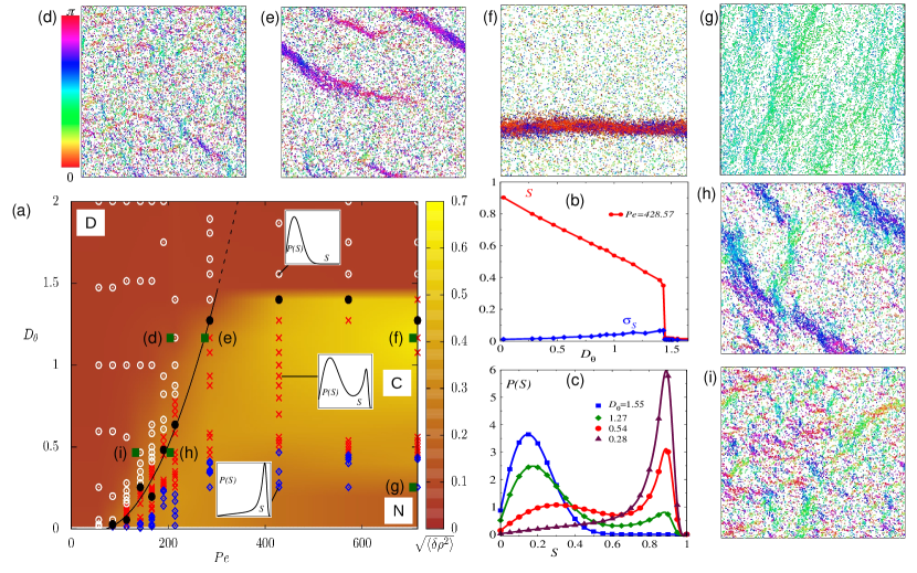
Figure 1: (a) Phase diagram in $(Pe,D_{\theta})$ plane with dimensionless activity $Pe=v_{0}/D_{r}r_{c}$ and orientational noise relative to alignment strength $D_{\theta}=2D_{r}/\mu J$ showing three distinct regions: disordered (D), coexistence (C) and nematic (N). The solid black line has the scaling form $D_{\theta}^{*}\sim Pe^{2}$ (see Sec.4 for derivation). (b) The nematic order $S$ (red line points) and standard deviation $\sigma_{s}$ (blue line points) as a function of $D_{\theta}$ at a fixed $Pe=428.57$. (c) The local probability distribution $P(S)$ at $Pe=428.57$ and various $D_{\theta}$ mentioned in the figure legend. The distributions are calculated using $S$ calculated over local coarse-grained volumes of linear dimension $10\,r_{c}$. (e-i) Representative configurations at parameter values marked by solid green boxes in the phase diagram in (a). The parameter values are $~{}(Pe,D_{\theta})=$ (142.85, 0.466), (214.28, 0.466), (714.28, 0.254), (714.28, 1.166), (285.71, 1.166), (214.28,1.166), respectively. The color palette to the left of Figure (d) denotes the heading directions of the particles in all the snapshots shown here.

3 Phase diagram

We begin our investigation by studying the steady states of the model in square geometry of size $L=200$ and $N=16000$, utilizing periodic boundary conditions (PBC). Fig.1(a) shows the phase diagram of the nematic-isotropic (NI) transition. The regions of the nematic phase (N) are denoted by blue diamonds, the region of nematic-isotropic coexistence (C) is indicated by red crosses, and the disordered isotropic phase (D) regions are marked by white open circles. The phase boundary between isotropic and coexistence is denoted by black-filled circles. The heat map in the phase diagram shows the amount of density fluctuations. This is calculated in coarse-grained volumes of linear dimension $10r_{c}$ using $\delta\rho=[\langle\rho^{2}\rangle-\langle\rho\rangle^{2}]^{1/2}$, and then averaging over the system size and all steady state configurations. As the color codes show, the density fluctuation is maximum in the coexistence. Its presence is significant even in the ordered nematic phase. The fluctuation is minimal in the homogeneous isotropic phase.

The three insets show the typical distributions of the scalar nematic order parameter corresponding to nematic (N), coexistence (C), and isotropic (D) regions. The black solid line indicates a $D_{\theta}\sim Pe^{2}$ boundary between the isotropic and nematic phases. An analytic description of the NI phase boundary $D_{\theta}\sim Pe^{2}$ is provided in the following section. The broken solid line indicates a breakdown of this simple estimate. As expected, the nematic phase is characterized by a giant number fluctuation [26, 28]. Deep inside the nematic phase, e.g., at $Pe=428.57$ and $D_{\theta}=0.28$ the system shows $\Delta n^{2}=\langle n^{2}\rangle-\langle n\rangle^{2}\sim n^{a}$ with $a\approx 1.8$. The steady-state pair correlation function $C(r)=1-b(r/L)^{\alpha}$ with $\alpha\approx 0.26$ [26, 42] signifies a clear violation of Porod’s law in the coexistence region. This captures a huge roughness of interfaces evidenced by large $(1-\alpha)$ characterizing a fluctuation-dominated phase separation.

The NI transition is captured using the dependence of the scalar order parameter $S$ and its standard deviation $\sigma_{s}=[\langle S^{2}\rangle-\langle S\rangle^{2}]^{1/2}$ on $D_{\theta}$, at a fixed $Pe$; see Fig.1(b). The local probability distribution $P(S)$ in Fig.1(c) shows an unimodal distribution with the maximum at small $S$ for large $D_{\theta}$, transforms into a bimodal distribution at intermediate $D_{\theta}$ values. This clearly indicates a phase coexistence, characterizing a first-order transition. At an even smaller $D_{\theta}$, the distribution becomes unimodal again, this time displaying a single maximum at large $S$, indicating a nematic phase.

Representative configurations are shown in Fig.1(d)-(i), with orientations distinguished by a color palette shown on the left of Fig.1(d). The parameter values associated with these configurations are marked by solid green squares on the phase diagram Fig.1(a). A typical configuration of the isotropic phase in Fig.1(d) shows an approximately homogeneous distribution of particles and their random orientations of heading direction. At a higher $Pe$, in Fig. 1(e), we observe a local clustering of particles in oriented bands. These bands display a higher nematic order. At an even higher $Pe$ in Fig.1(f), simulations show system-spanning bands with large nematic order coexisting with a uniform isotropic background. This corresponds to the bimodal distribution in $P(S)$ shown in Fig.1(c). Decreasing $D_{\theta}$, keeping $Pe$ unchanged, in Fig.1(g), we observe nice nematic order all through the system, corresponding to a homogeneous nematic fluid phase. The corresponding distribution $P(S)$ is unimodal with the maximum at large $S$. Again, in Fig.1(h), we show a typical configuration at a smaller $Pe$ and $D_{\theta}$, near the phase boundary, to find local nematic bands coexisting with an isotropic background. At an even smaller $Pe$, the system gets back to the isotropic phase in the presence of large density fluctuations; see Fig.1(i).

4 Mean field and hydrodynamic analysis

In this section, we proceed to develop a mean-field description of the observed NI phase transition. Using Eq.(2) it is straightforward to write the mean-field Fokker-Planck equation [26]

$$\partial_{t}p(\theta,t) = \partial_{\theta}\left[\gamma(n)\int_{0}^{2\pi}d\theta^{\prime}\sin[2(\theta-\theta^{\prime})]p(\theta,t)p(\theta^{\prime},t)\right]$$ (5)

$$+D_{r}\partial^{2}_{\theta}p,$$

where $\gamma(n)=2\mu Jn$, with $n=\pi r_{c}^{2}\rho$ denoting the mean number of nearest neighbors. The steady-state solution is

$$p_{st}(\theta)={\cal N}\exp\left[\frac{\gamma(n)S}{2D_{r}}\cos(2(\theta-\psi))\right].$$ (6)

where

$$S=\mid\int_{0}^{2\pi}d\theta p_{st}(\theta)\exp(i\,2\theta)\mid$$ (7)

denotes the scalar order parameter quantifying the degree of nematic order, and $\psi$ denotes the direction of broken symmetry.

From equations (7) and (6) we find the self-consistency relation $S=I_{1}\left[\frac{\gamma(n)S}{2D_{r}}\right]/I_{0}\left[\frac{\gamma(n)S}{2D_{r}}\right]$, where $I_{n}[.]$ denotes n-th order modified Bessel function of the first kind. For small $S$, a Taylor expansion gives, $S\approx\frac{\gamma(n)S}{4D_{r}}\left(1-\frac{\gamma^{2}(n)S^{2}}{64D_{r}^{2}}\right)$. Above the transition point, only one solution exists, $S=0$. Below it, $S=(2D_{\theta}/D_{\theta}^{(c)})(1-D_{\theta}/D_{\theta}^{(c)})^{1/2}$ where we used $D_{\theta}=2D_{r}/\mu J$ and the critical point

$$D_{\theta}^{(c)}=n=\pi r_{c}^{2}\rho$$ (8)

The above relations can be used to obtain an approximate mean-field evolution of the scalar order $dS/dt=-\partial{\cal A}/\partial S$ with [43]

$${\cal A}=-\frac{\alpha_{1}}{2}S^{2}+\frac{\alpha_{2}}{4}S^{4}$$ (9)

where $\alpha_{1}=1-\frac{D_{\theta}}{D_{\theta}^{(c)}}$ and $\alpha_{2}=\frac{1}{4}\left(\frac{D_{\theta}^{(c)}}{D_{\theta}}\right)^{2}$, with $D_{\theta}^{(c)}=A\rho$. This is only a partial description and predicts a continuous transition at the critical point $D_{\theta}^{(c)}$, in contrast to the first-order transition observed from numerical simulations. A better description must involve a coupled evolution of the tensor order parameter $Q_{ij}$ and local density $\rho$.

Towards that direction, in the following, we employ a phenomenological hydrodynamic approach [2, 17, 30] describing a coupled evolution of slow variables, the particle density $\rho({\bf r},t)$ and the local density of nematic order parameter $\Pi_{ij}({\bf r},t)=Q_{ij}({\bf r},t)\rho({\bf r},t)$, with

$${\bf Q}({\bf r},t)= \frac{S({\bf r},t)}{2}\begin{pmatrix}\cos 2\theta({\bf r},t)&\sin 2\theta({\bf r},t)\\ \sin 2\theta({\bf r},t)&-\cos 2\theta({\bf r},t)\end{pmatrix}$$

determined by the scalar order parameter $S({\bf r},t)$ describing the degree of nematic order and orientation $\theta({\bf r},t)$. Using active current $J^{(a)}_{i}=-Pe\partial_{j}\Pi_{ji}$ [4], the particle density field evolves as,

$$\partial_{t}\rho=Pe\partial_{i}\partial_{j}\Pi_{ji}+D\nabla^{2}\rho+\partial_{i}c_{i},$$ (10)

where $c_{i}$ denotes components of random current taken to be statistically isotropic and delta correlated. Also, $D$ denotes the diffusion constant. The evolution of nematic order follows [8, 9, 17, 4],

$$\partial_{t}\Pi_{ij} = [\alpha_{1}-\alpha_{2}\,{\rm Tr}(\Pi^{2})]\Pi_{ij}+D\nabla^{2}\Pi_{ij}$$ (11)

$$+\dfrac{Pe}{4}\left[\partial_{i}\partial_{j}-\frac{1}{2}\delta_{ij}\nabla^{2}\right]\rho+q_{ij}$$

Note that the coefficients $\alpha_{1}$ and $\alpha_{2}$ are density dependent. We included a spatiotemporal uncorrelated Gaussian tensorial noise $q_{ij}$, which is traceless and symmetric to denote thermal or active fluctuations. While the identification of $\alpha_{1}=\left(1-\frac{D_{\theta}}{D_{\theta}^{(c)}}\right)$ and $\alpha_{2}=\frac{1}{4}\left(\frac{D_{\theta}^{(c)}}{D_{\theta}}\right)^{2}$ with $D_{\theta}^{(c)}=A\rho$ is similar to Ref.9 in spirit but differs in detail. We perform a mean-field analysis in what follows.

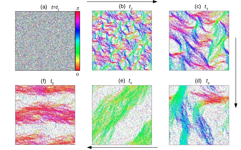
Figure 2: Typical configurations corresponding to the evolution after a quench from $D_{\theta}=2.8$ to $D_{\theta}=0.28$ at $Pe=428.57$ are shown. The color palette in (a) encodes orientations of particle heading directions. The black arrows show the direction of increasing time. At initial times, $t_{1}=0.007\,D_{r}^{-1}$, the system is in a homogeneous disordered phase (a). By $t_{2}=2.8\,D_{r}^{-1}$, thin nematic bands of higher density are formed. They are oriented in multiple directions (b). At a later time, $t_{3}=21\,D_{r}^{-1}$, these bands coarsen into thicker and longer branched patterns (c). At an even later time $t_{4}=350\,D_{r}^{-1}$, they coarsen into broader and system-spanning bands (d). By the time $t_{5}=12600\,D_{r}^{-1}$, steady-state system-spanning nematic bands appear (e). These bands break, form, and orient along spontaneously chosen directions that vary with time. For example, see another steady-state configuration at $t_{6}=19600\,D_{r}^{-1}$ (f). Here we use $N=64000$, $Pe=428.57$, $\rho r_{c}^{2}=0.4$, and $L=400r_{c}$.

First, let us consider the homogeneous limit of constant $\rho$. This leads to $\frac{dQ_{ij}}{dt}=[\alpha_{1}-\alpha_{2}{\rm Tr}(Q^{2})]Q_{ij}$ which suggests that the nematic phase can be stabilized only if $\alpha_{1}>0$, i.e., $D_{\theta}<D_{\theta}^{(c)}$. This sets the basic transition line but describes a continuous transition, in contrast to the first-order transitions observed in numerical simulations. The jump discontinuity in the scalar order parameter $S$ and the coexistence characterizing a first-order transition can be explained by incorporating the effects of activity-induced density fluctuations [44, 45] through the hydrodynamic equations and a renormalized mean-field (RMF) method [46]. A homogeneous steady-state solution of these equations predicts a transition where $\alpha_{1}(\rho)$ changes sign. Consider a small fluctuation in density $\delta\rho$ such that $\rho=\rho_{0}+\delta\rho$ arising due to activity to express $\alpha_{1}(\rho)=\alpha_{1}^{0}+{\alpha^{\prime}}_{1}^{0}\delta\rho$ where $\alpha_{1}^{0}$ and ${\alpha^{\prime}}_{1}^{0}$ are $\alpha_{1}$ and its derivative evaluated at $\rho_{0}$. Similarly, $\alpha_{2}(\rho)=\alpha_{2}^{0}+{\alpha^{\prime}}_{2}^{0}\delta\rho$ where $\alpha_{2}^{0}$ and ${\alpha^{\prime}}_{2}^{0}$ denote $\alpha_{2}$ and its derivative evaluated at $\rho_{0}$. A zero current steady state for the density evolution gives $\delta\rho\approx PeS/D$. Using this in the homogeneous mean-field limit of Eq.(11), we find

$$\partial_{t}S=[u_{2}+u_{3}S-u_{4}S^{2}]S.$$ (12)

This equation can be expressed as a free energy minimizing kinematics $\partial_{t}S=-\partial{\cal F}/\partial S$ with

$${\cal F}=-\frac{u_{2}}{2}S^{2}-\frac{u_{3}}{3}S^{3}+\frac{u_{4}}{4}S^{4},$$ (13)

keeping up to $S^{4}$ order term. In the above equation where $u_{2}=\alpha_{1}^{0}$, $u_{3}={\alpha^{\prime}}_{1}^{0}Pe/D$ and $u_{4}=\alpha_{2}^{0}$.

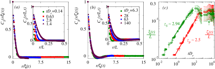
Figure 3: The nematic and density autocorrelation $C_{S}(r)$ ($a$) and $C_{\rho}(r)$ ($b$) during quench from $D_{\theta}=2.8$ to $D_{\theta}=0.28$ at $Pe=428.57$. Insets show the correlations plotted against $r/L$. The main plots show data collapse by scaling separation $r$ by dynamic correlation lengths $\xi(t)$ ($a$) and $\zeta(t)$ ($b$). $(c)$ The correlation lengths exhibit distinctive power-law growths $\xi(t)\sim t^{1/z_{\rho}}$ and $\zeta(t)\sim t^{1/z_{S}}$, where dynamic exponents $z_{\rho}=2.5$ and $z_{S}=2.94$. Coarse-grained cells of linear dimension $5\,r_{c}$ are used to calculate the coarse-grained correlations utilizing simulation results as in Fig.2.

Clearly, the active fluctuation in particle density generates the cubic term in $S$ in the effective free energy density, resulting in a first-order NI transition. At the transition, the scalar order parameter jumps from $S=0$ to

$$S_{c}=\frac{2}{3}\frac{{\alpha^{\prime}}_{1}^{0}}{\alpha_{2}^{0}}\frac{Pe}{D}.$$ (14)

The transition points change with $Pe$ to give the transition line

$$D_{\theta}^{\ast}=D_{\theta}^{(c)}\left[1+\frac{2}{9}\frac{({\alpha^{\prime}}_{1}^{0})^{2}}{\alpha_{2}^{0}}\left(\frac{Pe}{D}\right)^{2}\right],$$ (15)

increasing quadratically with $Pe$, see the black solid line in Fig.1(a). However, even the activity-induced increased density fluctuations fail to sustain the nematic order at higher $D_{\theta}$ ($D_{\theta}\gtrsim 1.4$). Therefore, the onset of nematic order with increasing $Pe$ disappears. This leads to a $Pe$-independent phase boundary. In fact, at these $D_{\theta}$ values, the density fluctuation gets suppressed, and one gets a homogeneous isotropic phase. This can be observed from the heat map in Fig.1(a). The NI transition is purely active; it vanishes in the limit of $Pe\to 0$ with the vanishing of $S_{c}$.

Before closing this section, certain comments are in order. We note that the observed first-order transition relies crucially on the reciprocal and additive nature of interaction implemented within the Lebowhl-Lasher model. Due to the additivity, the mean coupling strength $\gamma(n)$ in Eq.(5) depends on the mean number of neighbors of any particle. Thus $\gamma(n)\propto\rho$, which in turn leads to $D_{\theta}^{(c)}\propto\rho$. This provided the link of density fluctuation to the order parameter, leading to the first-order transition with the above mean-field description. If the alignment depended only on the average local orientation, the effective alignment strength $\gamma(n)$ would have been independent of the density $\rho$. This would decouple the nematic orientation from density fluctuations, snapping the link of density fluctuation to order parameters. The theory would then predict a continuous NI transition, as was observed before for non-reciprocal interaction models [26]. Within the Lebowhl-Lasher model implemented in the current study, the first-order ordering transition precludes the continuous transition as $D_{\theta}^{\ast}>D_{\theta}^{(c)}.$

5 Phase ordering kinematics

Having established the phenomenology of the NI transition, we now aim to understand the coarsening kinematics of the nematic order. Towards this end, we present our numerical results of the growth kinetics following a quench from an isotropic and homogeneous initial state at $D_{\theta}=2.8$ to $D_{\theta}=0.28$ in which the system gets to a steady-state nematic order at a fixed $Pe=428.57$. For better statistics, in the quench studies, we use a larger system with $N=64000$. Fig.2 shows a typical series of snapshots depicting this evolution. As time progresses, highly ordered high-density domains form, with their typical size increasing over time. In the beginning, the homogeneous isotropic state shows instability through the formation of nematically ordered filaments crisscrossing each other; see Fig.2(b). The small filaments merge and coarsen with time, as shown in Fig.2(c) and (d). At a late time, one finds dynamic system-spanning bands of nematically ordered regions; see Fig.2(e) and (f). In the steady state, the local undulations in nematic bands make them unstable toward breaking, and one finds repeated formation, breaking, and reorientations of such bands with time [10, 9].

To quantify these observations, we track the spatial nematic order parameter autocorrelation $C_{S}(r,t)$ and the density autocorrelation $C_{\rho}(r,t)$ as the system relaxes towards its final ordered state. Here $r=|{\bf r}|$ denotes the separation between coarse-grained regions of linear dimension $5r_{c}$. The correlation functions are defined as follows:

$$C_{S}(r,t)=\frac{Tr\langle{\bf Q}(r,t){\bf Q}(0,t)\rangle}{Tr\langle{\bf Q}^{2}(0,t)\rangle},$$ (16)

and

$$C_{\rho}(r,t)=\frac{\langle\delta\rho(r,t)~{}\delta\rho(0,t)\rangle}{\langle\delta\rho^{2}(0,t)\rangle}$$ (17)

where $\delta\rho(r)=\rho(r)-\rho_{0}$. Rescaling the separations by correlation lengths $\xi(t)$ and $\zeta(t)$, we obtain nice data collapse for both correlation functions, shown in the main figures of Fig.3(a) and (b). Both the correlation lengths, $\zeta(t)$ and $\xi(t)$, increase over time, following power laws $\xi(t)\sim{t}^{1/z_{s}}$ and $\zeta(t)\sim t^{1/z_{\rho}}$, with dynamic exponents $z_{s}\approx 2.94$ and $z_{\rho}\approx 2.5$. These values are slightly smaller than $3$ but larger than $2$. This bound is consistent with the earlier non-stochastic hydrodynamic calculations [41]. However, Ref.[41], in the absence of stochasticity, obtained the same growth law exponent for both the density and order parameter coarsening with a value $\approx 2.38$. This estimate differs from our findings of distinct dynamic exponents. Moreover, our stochastic calculations clearly predict two slightly different exponents $z_{s}$ and $z_{\rho}$ within the same overall bound $2<z_{s},\,z_{\rho}<3$. Note that the dynamical exponent $2$ characterizes the diffusive non-conserved dynamics in model A, and the exponent $3$ corresponds to the conserved model B dynamics [43]. The density field by itself follows conserved dynamics, while the nematic order parameter, being non-conserved, is expected to follow model A-like dynamics. The above analysis suggests that the dynamic exponents of the coupled evolution of density and nematic fields give rise to two distinct exponents with unique, non-overlapping values that fall between the limits of conserved and non-conserved dynamics.

6 Conclusions

We presented a comprehensive phase diagram as a function of activity $Pe$ and relative orientational noise $D_{\theta}$ for the nematic-isotropic transition in dry active nematics with reciprocal alignment interaction. The additive nature of the interaction ensures a first-order transition via coupling of nematic order to density fluctuations, confirmed through hydrodynamic theory and renormalized mean-field arguments.

It is intriguing that despite zero macroscopic velocity, the phase behavior of these apolar SPPs shows intricate dependence on $Pe$. Our theoretical analysis predicts a phase boundary $D_{\theta}\sim Pe^{2}$, aligning well with simulation results up to $D_{\theta}\approx 1.4$. Beyond this, local density increases fail to sustain nematic order, resulting in a $Pe$-independent boundary. The scalar order parameter shows a discontinuous jump proportional to $Pe$ at the transition, disappearing in the passive particle limit of $Pe\to 0$. We identify a broad parameter regime of phase coexistence. Deep within the nematic phase, the nematic bands are inherently unstable, exhibiting giant fluctuations and turbulent dynamics due to their continuous formation and breakup.

We investigated phase ordering kinetics by quenching from the isotropic to nematic phase, revealing coarsening patterns with growing correlation lengths as $t^{1/z}$ in nematic order and density fluctuations. Scaling laws exhibited two distinct exponents, $z_{s}\approx 2.94$ for nematic order and $z_{\rho}\approx 2.5$ for density, both falling within the bounds $2<z_{s},\,z_{r}<3$, consistent with earlier mean-field hydrodynamic predictions [41].

In conclusion, we obtained a comprehensive phase diagram for reciprocal alignment in active nematics, supported by theoretical predictions for the observed transition and phase boundaries. The coarsening dynamics showed dynamic exponents with values in between the exponents for non-conserved and conserved dynamics. The extent to which this phenomenology holds for non-reciprocal interactions warrants further investigation.

Author Contributions

DC designed the study. AS performed all the numerical calculations under the supervision of DC. DC and AS wrote the paper.

Conflicts of interest

There are no conflicts to declare.

References

- [1] R. Aditi Simha and Sriram Ramaswamy. Hydrodynamic fluctuations and instabilities in ordered suspensions of self-propelled particles. Phys. Rev. Lett., 89(5):058101, 2002.
- [2] S. Ramaswamy, R. Aditi Simha, and J. Toner. Active nematics on a substrate: Giant number fluctuations and long-time tails. Europhysics Letters, 62(2):196, apr 2003.
- [3] Sriram Ramaswamy. The Mechanics and Statistics of Active Matter. Annu. Rev. Condens. Matter Phys., 1(1):323–345, aug 2010.
- [4] M. C. Marchetti, J. F. Joanny, S. Ramaswamy, T. B. Liverpool, J. Prost, Madan Rao, and R. Aditi Simha. Hydrodynamics of soft active matter. Rev. Mod. Phys., 85(3):1143–1189, jul 2013.
- [5] F Julicher, K Kruse, J Prost, and J Joanny. Active behavior of the Cytoskeleton. Phys. Rep., 449(1-3):3–28, sep 2007.
- [6] J Prost, F Jülicher, and J-f Joanny. Active gel physics. Nat. Phys., 11(2):111–117, feb 2015.
- [7] Clemens Bechinger, Roberto Di Leonardo, Hartmut Löwen, Charles Reichhardt, Giorgio Volpe, and Giovanni Volpe. Active Particles in Complex and Crowded Environments. Rev. Mod. Phys., 88(4):045006, nov 2016.
- [8] Xia-qing Shi and Yu-qiang Ma. Deterministic endless collective evolvement in active nematics. preprint arXiv:1011.5408, 2010.
- [9] Xia-qing Shi, Hugues Chaté, and Yu-qiang Ma. Instabilities and chaos in a kinetic equation for active nematics. New J. Phys., 16(3):035003, mar 2014.
- [10] Sandrine Ngo, Anton Peshkov, Igor S Aranson, Eric Bertin, Francesco Ginelli, and Hugues Chaté. Large-scale chaos and fluctuations in active nematics. Physical review letters, 113(3):038302, 2014.
- [11] Tamás Vicsek, András Czirók, Eshel Ben-Jacob, Inon Cohen, and Ofer Shochet. Novel type of phase transition in a system of self-driven particles. Physical Review Letters, 75(6):1226, 1995.
- [12] Guillaume Grégoire and Hugues Chaté. Onset of Collective and Cohesive Motion. Phys. Rev. Lett., 92(2):025702, jan 2004.
- [13] H. Chaté, F. Ginelli, G. Grégoire, F. Peruani, and F. Raynaud. Modeling collective motion: Variations on the Vicsek model. Eur. Phys. J. B, 64(3-4):451, 2008.
- [14] John Toner and Yuhai Tu. Long-range Order in a 2d dynamic xy model: how birds fly together. Phys. Rev. Lett., 75(23):4326–4329, 1995.
- [15] Fernando Peruani, Andreas Deutsch, and Markus Bär. Nonequilibrium clustering of self-propelled rods. Phys. Rev. E, 74(3):030904, sep 2006.
- [16] Francesco Ginelli, Fernando Peruani, Markus Bär, and Hugues Chaté. Large-scale collective properties of self-propelled rods. Physical review letters, 104(18):184502, 2010.
- [17] Eric Bertin, Hugues Chaté, Francesco Ginelli, Shradha Mishra, Anton Peshkov, and Sriram Ramaswamy. Mesoscopic theory for fluctuating active nematics. New J. Phys., 15(8):085032, aug 2013.
- [18] Daniel L. Blair, T. Neicu, and A. Kudrolli. Vortices in vibrated granular rods. Phys. Rev. E, 67:031303, Mar 2003.
- [19] Vijay Narayan, Sriram Ramaswamy, Narayanan Menon, The Caspt, and The Caspt. Long-Lived Giant Number Fluctuations. Science (80-. )., 317(July):105–108, 2007.
- [20] Oleksandr Chepizhko, David Saintillan, and Fernando Peruani. Revisiting the emergence of order in active matter. Soft Matter, 17(11):3113–3120, 2021.
- [21] Dirk Helbing, Illés Farkas, and Tamás Vicsek. Simulating dynamical features of escape panic. Nature, 407(6803):487–490, sep 2000.
- [22] Suropriya Saha, Jaime Agudo-Canalejo, and Ramin Golestanian. Scalar Active Mixtures: The Nonreciprocal Cahn-Hilliard Model. Phys. Rev. X, 10(4):41009, 2020.
- [23] A. V. Ivlev, J. Bartnick, M. Heinen, C. R. Du, V. Nosenko, and H. Löwen. Statistical mechanics where Newton’s third law is broken. Phys. Rev. X, 5(1):011035, 2015.
- [24] Michel Fruchart, Ryo Hanai, Peter B. Littlewood, and Vincenzo Vitelli. Non-reciprocal phase transitions. Nature, 592(7854):363–369, apr 2021.
- [25] Sarah A. M. Loos, Sabine H. L. Klapp, and Thomas Martynec. Long-range Order and Directional Defect Propagation in the Nonreciprocal XY Model with Vision Cone Interactions. Phys. Rev. Lett., 130(19):198301, 2022.
- [26] Arpan Sinha and Debasish Chaudhuri. How reciprocity impacts ordering and phase separation in active nematics? Soft Matter, 20(i):788–795, 2024.
- [27] R. Aditi Simha and Sriram Ramaswamy. Hydrodynamic fluctuations and instabilities in ordered suspensions of self-propelled particles. Phys. Rev. Lett., 89:058101, Jul 2002.
- [28] Shradha Mishra and Sriram Ramaswamy. Active Nematics Are Intrinsically Phase Separated. Phys. Rev. Lett., 97(9):090602, aug 2006.
- [29] Hugues Chaté, Francesco Ginelli, and Raúl Montagne. Simple model for active nematics: Quasi-long-range order and giant fluctuations. Physical review letters, 96(18):180602, 2006.
- [30] Rakesh Das, Manoranjan Kumar, and Shradha Mishra. Order-disorder transition in active nematic: A lattice model study. Sci. Rep., 7(1):7080, aug 2017.
- [31] Fernando Peruani, Jörn Starruß, Vladimir Jakovljevic, Lotte Sogaard-Andersen, Andreas Deutsch, and Markus Bär. Collective Motion and Nonequilibrium Cluster Formation in Colonies of Gliding Bacteria. Phys. Rev. Lett., 108(9):098102, feb 2012.
- [32] Hans Gruler, Manfred Schienbein, Kurt Franke, and Anne de Boisfleury-chevance. Migrating Cells: Living Liquid Crystals. Mol. Cryst. Liq. Cryst. Sci. Technol. Sect. A. Mol. Cryst. Liq. Cryst., 260(1):565–574, feb 1995.
- [33] H Gruler, U Dewald, and M Eberhardt. Nematic liquid crystals formed by living amoeboid cells. The European Physical Journal B-Condensed Matter and Complex Systems, 11:187–192, 1999.
- [34] Lakshmi Balasubramaniam, René-Marc Mège, and Benoît Ladoux. Active nematics across scales from cytoskeleton organization to tissue morphogenesis. Curr. Opin. Genet. Dev., 73:101897, apr 2022.
- [35] Yilin Wu, A. Dale Kaiser, Yi Jiang, and Mark S. Alber. Periodic reversal of direction allows Myxobacteria to swarm. Proc. Natl. Acad. Sci., 106(4):1222–1227, jan 2009.
- [36] Matthias Theves, Johannes Taktikos, Vasily Zaburdaev, Holger Stark, and Carsten Beta. A Bacterial Swimmer with Two Alternating Speeds of Propagation. Biophys. J., 105(8):1915–1924, oct 2013.
- [37] Jörn Starruß, Fernando Peruani, Vladimir Jakovljevic, Lotte Sogaard-Andersen, Andreas Deutsch, and Markus Bär. Pattern-formation mechanisms in motility mutants of Myxococcus xanthus. Interface Focus, 2(6):774–785, dec 2012.
- [38] Greg M Barbara and James G Mitchell. Bacterial tracking of motile algae. FEMS Microbiol. Ecol., 44(1):79–87, may 2003.
- [39] Barry L. Taylor and D. E. Koshland. Reversal of Flagellar Rotation in Monotrichous and Peritrichous Bacteria: Generation of Changes in Direction. J. Bacteriol., 119(2):640–642, aug 1974.
- [40] P. A. Lebwohl and G. Lasher. Nematic-liquid-crystal order—a Monte Carlo calculation. Phys. Rev. A, 6:426–429, Jul 1972.
- [41] Shradha Mishra, Sanjay Puri, and Sriram Ramaswamy. Aspects of the density field in an active nematic. Philosophical Transactions of the Royal Society A: Mathematical, Physical and Engineering Sciences, 372(2029):20130364, 2014.
- [42] Dibyendu Das and Mustansir Barma. Particles Sliding on a Fluctuating Surface: Phase Separation and Power Laws. Phys. Rev. Lett., 85(8):1602–1605, aug 2000.
- [43] P. M. Chaikin and T. C. Lubensky. Principles of Condensed Matter Physics. Cambridge University Press, Cambridge, jun 1995.
- [44] Jing-Huei Chen, T. C. Lubensky, and David R. Nelson. Crossover near fluctuation-induced first-order phase transitions in superconductors. Phys. Rev. B, 17(11):4274–4286, jun 1978.
- [45] B. I. Halperin, T. C. Lubensky, and Shang-keng Ma. First-Order Phase Transitions in Superconductors and Smectic-A Liquid Crystals. Phys. Rev. Lett., 32(6):292–295, feb 1974.
- [46] Wei-Lin Tu. Renormalized Mean Field Theory, pages 21–31. Springer Singapore, Singapore, 2019.