Fair Set Cover

Abstract.

The potential harms of algorithmic decisions have ignited algorithmic fairness as a central topic in computer science. One of the fundamental problems in computer science is Set Cover, which has numerous applications with societal impacts, such as assembling a small team of individuals that collectively satisfy a range of expertise requirements. However, despite its broad application spectrum and significant potential impact, set cover has yet to be studied through the lens of fairness.

Therefore, in this paper, we introduce Fair Set Cover, which aims not only to cover with a minimum-size set but also to satisfy demographic parity in its selection of sets. To this end, we develop multiple versions of fair set cover, study their hardness, and devise efficient approximation algorithms for each variant. Notably, under certain assumptions, our algorithms always guarantees zero-unfairness, with only a small increase in the approximation ratio compared to regular set cover. Furthermore, our experiments on various data sets and across different settings confirm the negligible price of fairness, as (a) the output size increases only slightly (if any) and (b) the time to compute the output does not significantly increase.

1. Introduction

The abundance of data, coupled with AI and advanced algorithms, has revolutionized almost every aspect of human life. As data-driven technologies take root in our lives, their drawbacks and potential harms become increasingly evident. Subsequently, algorithmic fairness has become central in computer science research to minimize machine bias. However, despite substantial focus on fairness in predictive analysis and machine learning (Barocas et al., 2017; Mehrabi et al., 2021; Pessach and Shmueli, 2022), traditional combinatorial optimization has received limited attention (Wang et al., 2022). Nevertheless, combinatorial problems such as ranking (Asudeh et al., 2019), matching (Esmaeili et al., 2023; García-Soriano and Bonchi, 2020), resource allocation (Donahue and Kleinberg, 2020; Blanco and Gázquez, 2023; Jiang et al., 2021), and graph problems of influence maximization (Tsang et al., 2019) and edge recommendation (Swift et al., 2022; Bashardoust et al., 2023) have massive societal impact.

In this paper, we study the Set Cover problem through the lens of fairness. As one of Karp’s 21 NP-complete problems with various forms, set cover models a large set of real-world problems  (Vemuganti, 1998; ReVelle et al., 1976), ranging from airline crew scheduling (Rubin, 1973) and facility location (such as placing cell towers) to computational biology (Cho et al., 2012) and network security (Ge, 2010), to name only a few. Beyond its classical application examples, in the real world, set cover is frequently used to model problems that (either directly or indirectly) impact societies and human beings. In such settings, it is vital to ensure that the set cover optimization (a) does not cause bias and discrimination against some (demographic) groups, and (b) promotes social values such as equity and diversity. We further motivate the problem with a real-world application in Example 1 for Team of Experts Formation.

Example 1.

Consider an institution that wants to assemble a team of experts (e.g., a data science company that wants to hire employees) that collectively satisfy a set of skills (e.g., {python, sql, data-visualization, statistics, deep-learning, data-wrangling, $\cdots$}), i.e., for any skill, there must be at least one team member who has expertise in that skill. Naturally, the institution’s goal is to cover all the skills with the smallest possible team. However, due to the historical biases in the society, such an approach can cause discrimination by mostly selecting the team members from the privileged groups. Unfortunately, examples of such cases (and their consequences) are well-known in the real world. For instance, investigating an incident where HP webcams failed to track black individuals (Simon, 2009), revealed that HP engineers were mostly white-male and that caused the issue (Townsend, 2017). On the flip side, promoting social values such as diversity are always desirable in problems such as team formation (e.g., the data science company would like to ensure diversity in their hiring). In other words, not only do they want to satisfy all skills, but they also want to have an equal (or proportionate) representation of various demographic groups in the assembled team.

Motivated by Example 1 and other social applications of set cover, outlined in § 2, in this paper we introduce fair set cover, where the objective is to find a smallest collection of sets to cover a universe of items, while ensuring (weighted) parity in the selection of sets from various groups.

Summary of contributions

In this paper, we revisit the set cover problem through the lens of group fairness. Our main contributions are as follows.

• (§ 2, § 3) Demonstrating some of its applications, we propose the (unweighted and weighted) fair set cover problem, and study its complexity and hardness of approximation. We formulate fairness based on demographic parity in a general form that can be used to enforce count parity, as well as ratio parity, in selection among a set of binary or non-binary demographic groups. While various related problems have been studied in the literature (see § 8), to the best of our knowledge, we are the first to formulate and study the problem of fair set cover.

• (§ 4, § 6) In the unweighted setting, we first propose a naive algorithm that achieves zero-unfairness but at a (large) cost of increasing the approximation-ratio by a factor of the number of groups. Next, we propose a greedy algorithm that, while guaranteeing fairness, has the same approximation ratio as of the regular set cover; however, its running time is exponential in the number of groups. Therefore, we propose a faster (polynomial) algorithm that still guarantees fairness but slightly increases the approximation ratio by a fixed factor of $\frac{e}{e-1}$.

• (§ 5, § 6) In the weighted setting, we follow the same sequence by first proposing a naive algorithm that guarantees fairness but at a cost of a major increase in the output size (approximation ratio). We then propose a greedy algorithm that improves the approximation ratio but runs in exponential time relative to the number of groups. Finally, we propose a faster algorithm but at the expense of a minor increase in the approximation ratio.

• (§ 4, § 5) We propose the intermediate problems of max $k$-color cover and its weighted version. We study the computational complexity and propose approximation algorithms for both weighted and unweighted versions.

• (§ 7) To validate our theoretical findings, we conduct comprehensive experiments on real and synthetic datasets, across various settings, including binary vs. non-binary groups and fairness based on equal count vs. ratio parity. In summary, our experiments verify that our algorithms can achieve fairness (zero unfairness) with a negligible (if any) increase in the output size, and a small increase in the run time.

2. Application Demonstration

Set cover is a common selection problem in the real world, where, for example, one aims to select a minimal set from several options (sets) that collectively satisfy a universe of requirements. Moreover, in social settings where the choices are related to social groups, it may be desirable to ensure equality (or other suitable proportion) while selecting from various groups in order to prevent social discrimination. In Example 1, we demonstrated an application of fair set cover for Team of Experts Formation. To demonstrate the application-span of our formulation, in the following, we briefly mention a few more applications.

Equal Base-rate in representative data sets

An equal base rate is defined as having an equal number of objects for different subgroups in the data set (Kleinberg et al., 2016). Satisfying equal base-rate is important for satisfying multiple fairness metrics in down-stream machine learning task. Consider the schema of a dataset of individual records (e.g., Chicago breast-cancer examination data), with a set of attributes $\mathbf{x}=\{x_{1},\cdots,x_{\eta}\}$, where $\text{dom}(x_{i})>1$ is the domain of $x_{i}$. In order to ensure representativeness in the data, suppose we would like to collect a minimal set that contains at least one instance from all possible level-$\ell$ value combinations. A level-$\ell$ combination is a value-combination containing $\ell$ attributes in $\mathbf{x}$. Each individual belongs to a demographic group (e.g., White, Black). In order to reduce potential unfairnesses for various groups (e.g., Chicago breast-cancer detection disparities (Hirschman et al., 2007)), it is required to satisfy equal base-rate in the dataset. This is an instance of fair set cover, where each row (individual record) in the data set, covers all level-$\ell$ combinations it matches with.

Another similar application is fair survey data collection. Consider a full-factorial experiment design (Atkinson et al., 2007), where the goal is to collect a minimum size survey data in a way that at least one instance from each combination of values is surveyed. While satisfying the full-factorial design requirement, it would be desirable to equalize the participants from various demographic groups to obtain a diverse opinion, creating an instance of fair set cover.

Business license distribution

Issuing a minimum number of business licences (e.g., cannabis dispensary) while covering the population of a city is a challenging task for the City Office. Each business location covers regions within a certain (travel time) range. Besides coverage, equity is a critical constraint in these settings. For example, disparity against Black-owned cannabis dispensaries in Chicago is a well-known issue (Vinicky, 2022). Formulating and solving this problem as a fair set cover instance will resolve the disparity issues.

In Social Networks a similar application is influencer selection, where companies would like to select a small set of “innfluencers” to reach out to their target application. Specifically, once an influencer (aka content creator) post a content about a product, their followers view it. However, the company might also want to send their products to a diverse set of influencer, to prevent visual biases in their advertisement (Marcelle, [n. d.]).

In Appendix A, we provide additional applications of fair set cover in developing recommendation indices and fair clustering.

3. Preliminaries

3.1. Problem definition

We are given a universe of $n$ elements $U=\{e_{1},e_{2},\ldots,e_{n}\}$, a family of $\mu$ sets $\mathcal{S}=\{S_{1},S_{2},\ldots,S_{\mu}\}$, where $\cup_{i=1}^{\mu}S_{i}=U$. We are also given a set of $k$ demographic groups $\mathcal{G}=\{\mathbf{g}_{1},\ldots,\mathbf{g}_{k}\}$ (e.g., {white-male, black-female,... }), while each set $S_{j}$ in the family $\mathcal{S}$ belongs to a specific demographic group $\mathbf{g}(S_{j})\in\mathcal{G}$. In the rest of this paper, we interchangeably refer to the group of a set as its color. Let $\mathcal{S}_{h}\subseteq\mathcal{S}$ be the family of sets from $\mathcal{S}$ with color $\mathbf{g}_{h}\in\mathcal{G}$. Let $m_{h}$ be the number of sets of color $\mathbf{g}_{h}$ in $\mathcal{S}$, i.e., $m_{h}=|\mathcal{S}_{h}|$. A cover $X\subseteq\mathcal{S}$ is a subset of $\mathcal{S}$ such that for any $e\in U$ there exists a set $S\in X$ with $e\in S$. In other words, $X$ is a cover if $\bigcup_{s_{i}\in X}=U$. To simplify the notation, for a family of sets $X\subseteq\mathcal{S}$, we define $X\cap U=(\bigcup_{S\in X}S)\cap U$.

Fairness definition

Following Example 1 and the applications demonstrated in § 2, we adopt the group-fairness notion of demographic parity, as the (weighted) parity between the number of sets selected from each group. Specifically, given the non-negative coefficients $\{f_{1},\cdots,f_{k}\}$ such that $\sum\limits_{h=1}^{k}f_{h}=1$, a cover $X$ is called a fair cover if, for all groups $\mathbf{g}_{h}\in\mathcal{G}$:

$$\big{|}\{X\cap\mathcal{S}_{h}\}\big{|}=f_{h}\,\big{|}X\big{|}$$

Two special cases based on this definition are the following:

• Count-parity: when $f_{h}=\frac{1}{k}$, $\forall\mathbf{g}_{h}\in\mathcal{G}$, a fair set cover contains equal number from each group.

• Ratio-parity: when $f_{h}=\frac{m_{h}}{\mu}$, $\forall\mathbf{g}_{h}\in\mathcal{G}$, a fair set cover maintains the original ratios of groups in $\mathcal{S}$.

Note that our fairness definition is not limited to the above cases, and includes any fractions (represented as rational numbers) specified by non-negative coefficients $f_{h}$ such that $\sum_{h=1}^{k}f_{h}=1$.

Definition 0 (Generalized Fair Set Cover problem (GFSC)).

Given a universe of $n$ elements $U$, a set of $k$ groups $\mathcal{G}=\{\mathbf{g}_{1},\ldots,\mathbf{g}_{k}\}$, a fraction $f_{h}$ for each $\mathbf{g}_{h}\in\mathcal{G}$ such that their sum is equal to $1$, and a family of $\mu$ subsets $\mathcal{S}$, such that each $S\in\mathcal{S}$ is associated with a group $\mathbf{g}(S)\in\mathcal{G}$, the goal is to compute a fair cover of minimum size.

In the next sections, we denote the optimum fair cover with $X^{*}$.

Next, we consider the weighted version of the GFSC problem. Let $w:\mathcal{S}\rightarrow\mathbb{R}^{+}$ be a weighted function over the sets in $\mathcal{S}$. By slightly abusing the notation, for a family of sets $C\subseteq\mathcal{S}$, we define $w(C)=\sum_{S\in C}w(S)$. The goal is to find a fair cover such that the selected sets in the cover has the smallest sum of weights.

Definition 0 (Generalized Fair Weighted Set Cover problem (GFWSC)).

Given a universe of $n$ elements $U$, a set of $k$ groups $\mathcal{G}=\{\mathbf{g}_{1},\ldots,\mathbf{g}_{k}\}$, a fraction $f_{h}$ for each $\mathbf{g}_{h}\in\mathcal{G}$ such that their sum is equal to $1$, a family of $\mu$ subsets $\mathcal{S}$, such that each $S\in\mathcal{S}$ is associated with a group $\mathbf{g}(S)\in\mathcal{G}$, and a weighted function $w:\mathcal{S}\rightarrow\mathbb{R}^{+}$ the goal is to compute a fair cover $X_{w}$ such that $\sum_{S\in X_{w}}w(S)$ is minimized.

In the rest of the paper, we denote the optimum solution for the GFWSC problem with $X_{w}^{*}$.

Under the count-parity fairness model, we call our problems, the Fair Set Cover (FSC) problem, and the Fair Weighted Set Cover (FWSC) problem, respectively. Even though the GFSC and GFWSC problems are more general than FSC and FWSC, respectively, the algorithmic techniques to solve FSC and FWSC can straightforwardly be extended to handle GFSC and GFWSC with (almost) the same guarantees. In order to simplify the analysis, in the next sections we focus on FSC and FWSC. Then in § 6, we describe how our algorithms can be extended to handle GFSC and GFWSC.

It is straightforward to show that FSC is NP-Complete. In Appendix B, we also show that in the general case, FSC cannot be approximated with any non-trivial approximation factor in polynomial time unless $\mathsf{P}\neq\mathsf{NP}$.

Theorem 3.

The FSC problem is NP-Complete. Furthermore, there is no polynomial time algorithm for the FSC problem with approximation ratio $f(n)$, where $f(\cdot)$ is any computable non-decreasing function such that $1\leq f(n)=o(n)$, unless $\mathsf{P}=\mathsf{NP}$.

Assumption.  In the general case, we cannot hope for a polynomial time approximation algorithm for the FSC problem. However, if there are enough sets from each group, then in the next sections we design efficient algorithms with provable approximation guarantees. More formally, for the FSC problem, we assume that every group contains at least $\Omega(\log n)\frac{|X^{*}|}{k}$ sets. Notice that we do not know the value of $|X^{*}|$ upfront. However, if this assumption is satisfied then all our approximation algorithms are correct. For simplicity, in the next sections we also assume that every group has the same number of sets, i.e., for every group $\mathbf{g}_{j}$ it holds that $m_{j}=m$. Hence, $\mu=mk$. This only helps us to analyze our algorithms with respect to only three variables, $m,k,n$. All our algorithms can be extended to more general cases (where each color does not contain the same number of sets). We further highlight it in § 7, where we run experiments on datasets with $m_{i}\neq m_{j}$ for $i\neq j$.

4. Fair Set Cover

4.1. Naive Algorithm

We first describe a naive algorithm for the FSC problem with large approximation ratio. We execute the greedy algorithm for the set cover problem and let $X$ be the set cover we get. If $X$ satisfies the fairness requirements, then we return $X$. If $X$ does not satisfy the fairness requirements, we arbitrarily add the minimal number of sets from each color to equalize the number of sets from each color in our final cover, which makes the approximation ratio $k(\ln n+1)$.

Lemma 0.

There exists a $\big{(}k(\ln n+1)\big{)}$-approximation algorithm for the FSC problem that runs in $O(m\cdot k\cdot n)$ time.

4.2. Greedy Algorithm

The main issue with the Naive algorithm is that its approximation ratio is linear to $k$. In this subsection we propose an algorithm for the FSC problem whose approximation ratio does not depend on $k$. For simplicity of explanation, we describe our algorithm for the case we have only two demographic groups, i.e., $\mathcal{G}=\{\mathbf{g}_{1},\mathbf{g}_{2}\}$. In the end, our algorithm can be extended almost verbatim to $k>2$ groups.

Let $X=\emptyset$ be the cover we construct and let $U^{-}=U$ be the set of uncovered elements. We repeat the following steps until $U^{-}=\emptyset$. In each iteration, we find the pair of sets $(S_{A},S_{B})$ such that i) sets $S_{A},S_{B}$ cover the maximum number of uncovered elements, i.e., $U^{-}\cap(S_{A}\cup S_{B})$ is maximized, and ii) set $S_{A}$ has color $\mathbf{g}_{1}$ and $S_{B}$ has color $\mathbf{g}_{2}$, i.e., $\mathbf{g}(S_{A})=\mathbf{g}_{1}$ and $\mathbf{g}(S_{B})=\mathbf{g}_{2}$. Once we find $S_{A},S_{B}$ we update the set $U^{-}$ removing the new covered element, $U^{-}\leftarrow U^{-}\setminus(S_{A}\cup S_{B})$, and we add $S_{A},S_{B}$ in $X$. In the end, after covering all elements ($U^{-}=\emptyset$), we return $X$.

Analysis

First, it is straightforward to see that $X$ is a fair cover. The algorithm stops when there is no uncovered element so $X$ is a cover. In every iteration, we add exactly one set of color $\mathbf{g}_{1}$ and one set of color $\mathbf{g}_{2}$, so $X$ is a fair cover.

Lemma 0.

$|X|\leq(\ln n+1)\cdot|X^{*}|$.

Proof:

For each pair $S_{A},S_{B}\in\mathcal{S}$, let $S_{A,B}=S_{A}\cup S_{B}$. We consider the following instance of the set cover problem. We define the set $U^{\prime}=U$ and $\mathcal{S}^{\prime}=\{S_{i,j}\mid S_{i}\in\mathcal{S}_{1},S_{j}\in\mathcal{S}_{2}\}$. Let $C^{*}$ be the optimum solution of the set cover instance $(U^{\prime},\mathcal{S}^{\prime})$. Any fair cover returned by our algorithm can be straightforwardly mapped to a valid set cover for $(U^{\prime},\mathcal{S}^{\prime})$. For example, if our algorithm selects a pair $S_{A},S_{B}$ then it always holds that $S_{A,B}\in\mathcal{S}^{\prime}$ and $|(S_{A}\cap S_{B})\cap U|=|S_{A,B}\cap U^{\prime}|$. Hence, by definition, we have $|C^{*}|\leq\frac{1}{2}|X^{*}|$.

Recall that the standard greedy algorithm for the set cover problem returns a $(\ln n+1)$-approximation. We show that our algorithm implements such a greedy algorithm and returns a $(\ln n+1)$-approximation in the set cover instance $(U^{\prime},\mathcal{S}^{\prime})$. At the beginning of an iteration $i$, without loss of generality, assume that our algorithm has selected the pairs $(S_{A_{1}},S_{B_{1}}),\ldots,(S_{A_{i-1}},S_{B_{i-1}})$, so the sets $S_{A_{1},B_{1}},\ldots,S_{A_{i-1},B_{i-1}}$ have been selected for the set cover instance $(U^{\prime},\mathcal{S}^{\prime})$. Let $U^{-}$ be the set of uncovered elements in $U^{\prime}$ at the beginning of the $i$-th iteration. Let $S_{A_{j},B_{j}}$ be the set in $\mathcal{S}^{\prime}$ that covers the maximum number of elements in $U^{-}$. We consider two cases.

If $S_{A_{j}}\notin\{S_{A_{1}},\ldots,S_{A_{i-1}}\}$ and $S_{B_{j}}\notin\{S_{B_{1}},\ldots,S_{B_{i-1}}\}$, then by definition our greedy algorithm selects the pair $(S_{A_{j}},S_{B_{j}})$ so the set $S_{A_{j},B_{j}}$ is added in the cover of the set cover instance $(U^{\prime},\mathcal{S}^{\prime})$.

Next, consider the case where $S_{A_{j}}\notin\{S_{A_{1}},\ldots,S_{A_{i-1}}\}$ and $S_{B_{j}}\in\{S_{B_{1}},\ldots,S_{B_{i-1}}\}$ (the proof is equivalent if the set $S_{A_{j}}$ has been selected before). Since there are enough sets from each group, let $S_{B_{h}}$ be a set with color $\mathbf{g}_{2}$ such that $S_{B_{h}}\notin\{S_{B_{1}},\ldots,S_{B_{i-1}}\}$. By definition, we have $|S_{A_{j},B_{h}}\cap U^{-}|\geq|S_{A_{j},B_{j}}\cap U^{-}|$. Our greedy algorithm selects the pair $S_{A^{*}},S_{B^{*}}$ such that $|(S_{A^{*}}\cup S_{B^{*}})\cap U^{-}|$ is maximized, and $S_{A^{*}}\notin\{S_{A_{1}},\ldots,S_{A_{i-1}}\}$, $S_{B^{*}}\notin\{S_{B_{1}},\ldots,S_{B_{i-1}}\}$. Hence, $|S_{A^{*},B^{*}}\cap U^{-}|=|(S_{A^{*}}\cup S_{B^{*}})\cap U^{-}|\geq|(S_{A_{j}}\cup S_{B_{h}})\cap U^{-}|\geq|(S_{A_{j}}\cup S_{B_{j}})\cap U^{-}|=|S_{A_{j},B_{j}}\cap U^{-}|$.

We conclude that in every iteration, our greedy algorithm computes a set $S_{A,B}$ that covers the most uncovered elements in $U^{\prime}$. Hence, $\frac{1}{2}|X|\leq(\ln n+1)|C^{*}|\leq(\ln n+1)\frac{1}{2}|X^{*}|\Leftrightarrow|X|\leq(\ln n+1)|X^{*}|$. $\square$

Notice that there exists $O(m_{1}m_{2})=O(m^{2})$ pairs of sets with different colors. At the beginning of the algorithm, for every pair of sets we compute the number of elements they cover in $O(m^{2}n)$ time. Each time we cover a new element we update the counters in $O(m^{2})$ time. In total, our algorithm runs in $O(m^{2}n)$ time.

This greedy algorithm can be extended to $k$ groups, straightforwardly. In each iteration, we find the $k$ sets of different color that cover the the most uncovered elements. The running time increases to $O(m^{k}n)$.

Theorem 3.

There exists an $(\ln n+1)$-approximation algorithm for the FSC problem that runs in $O(m^{k}n)$ time.

While our algorithm returns an $O(\log n)$-approximation, which is the best that someone can hope for the FSC, the running time depends exponentially on the number of groups $k$. Next, we propose two faster $O(\operatorname{poly}(n,m,k))$ time randomized algorithms with the same asymptotic approximation.

4.3. Faster algorithms

The expensive part of the greedy algorithm is the selection of $k$ sets of different color that cover the most uncovered elements, in every iteration. We focus on one iteration of the greedy algorithm. Intuitively, we need to find $k$ sets, each from a different color, that maximizes the coverage over the uncovered elements. We call this problem, max $k$-color cover. Formally,

Definition 0 (max $k$-color cover).

Consider a set $U^{-}\subseteq U$, called the set of uncovered elements, a family of sets $\mathcal{S}^{-}\subseteq\mathcal{S}$, called the sets not selected so far, and the value $k$ showing the number colors (groups) that sets belong to. Our goal is to select $k$ sets $X\subseteq\mathcal{S}^{-}$, one from each color, such that $\big{|}X\cap U^{-}\big{|}$ is maximized.

The max $k$-color cover problem is $\mathsf{NP}$-complete. The proof is straight-forward using the reduction from the traditional max $k$-cover (MC) problem by creating $k$ copies of each original set, while assigning each copy to a unique color. Now the max-cover problem has a solution with coverage $\ell$, if and only if the $k$-color MC has a solution with coverage $\ell$. Since max $k$-color cover is $\mathsf{NP}$-complete, we propose constant-approximation polynomial algorithms for it.

$\frac{1}{2}$- approximation algorithm

Inspired by (Ma and Zheng, 2021), where the authors also study a version of the max $k$-color cover problem (to design efficient algorithms for the fair regret minimizing set problem), we propose the following simple algorithm. We run the standard greedy algorithm for the max $k$-cover problem. Let $Y=U^{-}$ be the current set of uncovered elements in $U^{-}$ and let $C=\emptyset$ be the family of $k$ sets we return. The next steps are repeated until $|C|=k$ or $Y=\emptyset$. In each iteration, the algorithm chooses the set $S\in\mathcal{S}^{-}$ such that $|S\cap Y|$ is maximized. If $C$ contains another set with color $\mathbf{g}(S)$, then we remove $S$ and we continue with the next iteration of the algorithm. Otherwise, we add $S$ in $C$ and we update $Y=Y\setminus S$. If $Y=\emptyset$ and $C$ does not contain sets from all groups, we add in $C$ exactly one set per missing group.

Theorem 5.

There exists an $\frac{1}{2}$-approximation algorithm for the max $k$-color cover problem that runs in $O(n\mu)$ time.

Proof:

By definition $C$ contains one set from each group in $\mathcal{G}$, so it is a valid $k$-color cover. Let $S_{h}$ be the $h$-th set added in $C$. Without loss of generality, assume $\mathbf{g}(S_{h})=\mathbf{g}_{h}$, for $h=1,\ldots,k$. Let $O^{*}=\{O_{1},\ldots,O_{k}\}\subseteq\mathcal{S}^{-}$ be the optimum solution for the max $k$-color cover problem. Without loss of generality, assume that $\mathbf{g}(O_{h})=\mathbf{g}_{h}$, for $h=1,\ldots,k$. We have,

$$|C| =\sum_{i=1}^{k}\left|S_{i}\setminus(\cup_{h=1..i-1}S_{h}\right)|\geq\sum_{i=1}^{k}\left|O_{i}\setminus\cup_{h=1}^{i-1}S_{h}\right|\geq\sum_{i=1}^{k}\left|O_{i}\setminus C\right|$$

$$\geq|O^{*}|-|C|.$$

Hence $|C|\geq\frac{1}{2}|O^{*}|$. Each time we cover a new element, we update the number of uncovered elements in each set in $O(\mu)$ time. Hence, the algorithm runs in $O(n\mu)$ time. $\square$

$(1-\frac{1}{e})$-approximation algorithm

We design a randomized LP-based algorithm for the max $k$-color cover problem with better approximation factor. For every element $e_{j}\in U^{-}$ we define the variable $y_{j}$. For every set $S_{i}\in\mathcal{S}^{-}$ we define the variable $x_{i}$. Let $\mathcal{S}_{h}^{-}=\{S\in\mathcal{S}^{-}\mid S\in\mathcal{S}_{h}\}$. The next Integer Program represents an instance of the max $k$-color cover problem.

$$\max\sum_{j}y_{j}$$

$$\sum_{i:S_{i}\in\mathcal{S}^{-}_{h}}x_{i} =1,\quad\forall\mathbf{g}_{h}\in\mathcal{G}$$

$$\sum_{i:e_{j}\in S_{i}}x_{i} \geq y_{j},\quad\forall e_{j}\in U^{-}$$

$$x_{i}\in\{0,1\},\forall S_{i}\in\mathcal{S}^{-},\quad y_{j}\in\{0,1\},\forall e_{j}\in U^{-}$$

We then replace the integer variables to continuous ($x_{i}\in[0,1]$ and $y_{j}\in[0,1]$) and use a polynomial time LP solver to compute the solution of the LP relaxation. Let $x_{i}^{*}$, $y_{j}^{*}$ be the values of the variables in the optimum solution. For every group $\mathbf{g}_{h}\in\mathcal{G}$, we sample exactly one set from $\mathcal{S}^{-}_{h}$, using the probabilities $\{x_{i}^{*}\mid S_{i}\in\mathcal{S}^{-}_{h}\}$. Let $C$ be the family of $k$ sets we return.

Analysis

By definition $C$ contains exactly one set from every group $\mathbf{g}_{i}$. Next, we show the approximation factor.

Lemma 0.

An element $e_{j}$ is covered by a set in $C$ with probability at least $(1-\frac{1}{e})y_{j}^{*}$.

Proof:

By definition, $e_{j}$ is not covered by a set in $\mathcal{S}^{-}_{h}$ with probability

$$1-\sum_{i:e_{j}\in S_{i},S_{i}\in\mathcal{S}^{-}_{h}}x_{i}^{*}\leq e^{-\sum_{i:e_{j}\in S_{i},S_{i}\in\mathcal{S}^{-}_{h}}x_{i}^{*}}.$$

The inequality holds because of the well know inequality $1+x\leq e^{x}$ for every $x\in\mathbb{R}$. Hence,

$$Pr[e_{j}\notin C] =\prod_{\mathbf{g}_{h}\in\mathcal{G}}(1-\sum_{i:e_{j}\in S_{i},S_{i}\in\mathcal{S}^{-}_{h}}x_{i}^{*})\leq\prod_{\mathbf{g}_{h}\in\mathcal{G}}e^{-\sum_{i:e_{j}\in S_{i},S_{i}\in\mathcal{S}^{-}_{h}}x_{i}^{*}}$$

$$=e^{-\sum_{\mathbf{g}_{h}\in\mathcal{G}}\sum_{i:e_{j}\in S_{i},S_{i}\in\mathcal{S}^{-}_{h}}x_{i}^{*}}=e^{-\sum_{i:e_{j}\in S_{i}}x_{i}^{*}}\leq e^{-y_{j}^{*}}.$$

We conclude that $Pr[e_{j}\in C]\geq 1-e^{-y_{j}^{*}}\geq(1-\frac{1}{e})y_{j}^{*}$. $\square$

Using Lemma 6, we show our main result.

Lemma 0.

The expected number of elements covered by sets in $C$ is at least $(1-\frac{1}{e})\mathsf{OPT}$, where $\mathsf{OPT}$ is the number of covered elements in the optimum solution for the max $k$-color cover problem.

Proof:

Let $\mathsf{OPT}_{LP}=\sum_{j}y_{j}^{*}$ be the optimum solution of the LP above. Let $Z_{j}$ be a random variable which is $1$ if $e_{j}$ is covered in $C$, and $0$ otherwise. We have

$$E\Big{[}\sum_{j}Z_{j}\Big{]} =\sum_{j}E[Z_{j}]=\sum_{j}Pr[Z_{j}=1]=\sum_{j}Pr[e_{j}\in C]$$

$$\geq\sum_{j}(1-\frac{1}{e})y_{j}^{*}=(1-\frac{1}{e})\sum_{j}y_{j}^{*}=(1-\frac{1}{e})\mathsf{OPT}_{LP}$$

$$\geq(1-\frac{1}{e})\mathsf{OPT}.$$

$\square$

Let $\mathcal{L}(a,b)$ be the running time to solve an LP with $a$ constraints and $b$ variables. Our algorithm for the max $k$-color cover problem runs in $O(\mathcal{L}(n+k,2n+2\mu))$ time.

Putting everything together, we conclude with the next theorem.

Theorem 8.

There exists an expected $(1-\frac{1}{e})$-approximation algorithm for the max $k$-color cover problem that runs in $O(\mathcal{L}(n+k,2n+2\mu))$ time.

Faster algorithm for FSC

We combine the results from Theorem 3 and Theorem 8 (or Theorem 5) to get a faster algorithm for the FSC problem. More specifically, in each iteration of the greedy algorithm from Theorem 3 we execute the algorithm from Theorem 8 (or Theorem 5).

It is known (Young, 2008) that the greedy algorithm for the standard Set Cover problem, where in each iteration it selects a set that covers a $\beta$-approximation (for $\beta<1$) of the maximum number of uncovered elements returns a $\frac{1}{\beta}(\ln n+1)$-approximation. From the proof of Lemma 2 we mapped the FSC problem to an instance of the standard set cover problem, so the approximation ratio of our new algorithm is $\frac{e}{e-1}(\ln n+1)$ (or $2(\ln n+1)$).

The algorithm from Theorem 8 runs in $O(\mathcal{L}(n+k,2n+2m\cdot k))$. We execute this algorithm in every iteration of the greedy algorithm. In the worst case the greedy algorithm selects all sets in $\mathcal{S}$, so a loose upper bound on the number of iterations is $O(m)$. The number of iterations can also be bounded as follows. If $I_{\mathsf{Greedy}}$ is the number of iterations of the greedy algorithm, then by definition it holds that $k\cdot I_{\mathsf{Greedy}}\leq\frac{e}{e-1}(\ln n+1)|X^{*}|\Leftrightarrow I_{\mathsf{Greedy}}=O(\frac{|X^{*}|}{k}\log n)$.

Theorem 9.

There exists an expected $\frac{e}{e-1}(\ln n+1)$-approximation algorithm for the FSC problem that runs in $O(\frac{|X^{*}|}{k}\mathcal{L}(n+k,2n+2m\cdot k)\log n)$ time. Furthermore, there exists a $2(\ln n+1)$-approximation algorithm that runs in $O(|X^{*}|\cdot n\cdot m\cdot\log n)$ time.

5. Weighted Fair Set Cover

Throughout this section we define $\Delta=\frac{w_{\mathsf{max}}}{w_{\mathsf{min}}}$, where $w_{\mathsf{max}}=\max\{w(S_{i})|S_{i}\in\mathcal{S}\}$ and $w_{\mathsf{min}}=\min\{w(S_{i})|S_{i}\in\mathcal{S}\}$. In this section we need the assumption that for every group $\mathbf{g}_{h}\in\mathcal{G}$ there are at least $\Omega(\Delta\log n)\cdot\frac{|X^{*}|}{k}$ sets. As we had for the FSC, for simplicity we also assume that every group has the same number of sets denoted by $m$.

In Appendix C, we show that a naive algorithm for the FWSC, similar to the naive algorithm we proposed for the FSC returns a $k\Delta(\ln n+1)$-approximation algorithm that runs in $O(m\cdot k\cdot n)$ time. Next, we propose algorithms with better theoretical guarantees.

5.1. Greedy Algorithm

We design a greedy algorithm that returns a $\Delta(\ln n+1)$-approximation for the FWSC problem. For simplicity, we describe our algorithm for the case we have only two demographic groups, i.e., $\mathcal{G}=\{\mathbf{g}_{1},\mathbf{g}_{2}\}$. In the end, our algorithm can be extended almost verbatim to $k>2$ groups. Let $X_{w}=\emptyset$ be the cover we construct and let $U^{-}=U$ be the set of uncovered elements. We repeat the following steps until $U^{-}=\emptyset$. In each iteration, we find the pair of sets $(S_{A},S_{B})$ such that i) the ratio $\frac{w(S_{A})+w(S_{B})}{|(S_{A}\cup S_{B})\cap U^{-}|}$ is minimized, and ii) $\mathbf{g}(S_{A})=\mathbf{g}_{1}$ and $\mathbf{g}(S_{B})=\mathbf{g}_{2}$. Once we find $S_{A},S_{B}$ we update the set $U^{-}$ removing the new covered element, $U^{-}\leftarrow U^{-}\setminus(S_{A}\cup S_{B})$, and we add $S_{A},S_{B}$ in $X_{w}$. In the end, after covering all elements we return $X_{w}$.

The proof of the next Theorem can be found in Appendix C.

Theorem 1.

There exists a $\Delta(\ln n+1)$-approximation algorithm for the FWSC problem that runs in $O(m^{k}n)$ time.

5.2. Faster algorithm

The expensive part of the previous greedy algorithm is the selection of $k$ sets of different color to minimize the ratio of the weight over the number of new covered elements, in every iteration. We focus on one iteration of the greedy algorithm, solving an instance of the weighted max $k$-color cover problem. We are given a set of $n$ elements $U^{-}\subseteq U$, a family of $\mu$ sets $\mathcal{S}^{-}\subseteq\mathcal{S}$, a weight function $w:\mathcal{S}^{-}\rightarrow\mathbb{R}^{+}$, and a set of $k$ groups $\mathcal{G}$ such that every set belongs to a group. The goal is to select a family of exactly $k$ sets $X_{w}\subseteq\mathcal{S}^{-}$ such that i) $\frac{w(X_{w})}{|X_{w}\cap U^{-}|}$ is minimized, and ii) there exists exactly one set from every color $\mathbf{g}_{h}\in\mathcal{G}$. An efficient constant approximation algorithm for the weighted max $k$-color cover problem could be used in every iteration of the greedy algorithm to get an $O(\Delta\log n)$-approximation in $O(\operatorname{poly}(n,m,k))$ time.

Algorithm

We design a randomized LP-based algorithm for the weighted max $k$-color cover problem. We note that our new algorithm has significant changes compared to the LP-based algorithm we proposed for the unweighted case. The reason is that the objective of finding a fair cover $X_{w}$ that minimizes $\frac{w(X_{w})}{|X_{w}\cap U^{-}|}$ can not be represented as a linear constraint. Instead, we iteratively solve a constrained version of the weighted max $k$-color cover problem: For a parameter $\tau\in[1,n]$, the goal is to select a family of exactly $k$ sets $X_{w}\subset\mathcal{S}^{-}$ such that i) $w(X_{w})$ is minimized, ii) $|X_{w}\cap U^{-}|\geq\tau$, and iii) there exists exactly one set from every color $\mathbf{g}_{h}\in\mathcal{G}$ in $X_{w}$. The main idea of our algorithm is that for each $\tau=1,\ldots,n$, we compute efficiently an approximate solution for the constrained weighted max $k$-color cover problem. In the end, we return the best solution over all $\tau$’s.

For every $\tau=1,\ldots,n$, we solve an instance of the constrained weighted max $k$-color cover problem. The next Integer Program represents an instance of the constrained weighted max $k$-color cover problem with respect to $\tau$.

$$\min\sum_{S_{i}\in\mathcal{S}^{-}}w(S_{i})x_{i}$$

$$\sum_{i:S_{i}\in\mathcal{S}^{-}_{h}}x_{i} =1,\quad\forall\mathbf{g}_{h}\in\mathcal{G}$$

$$\sum_{i:e_{j}\in S_{i}}x_{i} \geq y_{j},\quad\forall e_{j}\in U^{-}$$

$$\sum_{e_{j}\in U^{-}}y_{j} \geq\tau$$

$$x_{i}\in\{0,1\},\forall S_{i}\in\mathcal{S}^{-},\quad y_{j}\in\{0,1\},\forall e_{j}\in U^{-}$$

We then replace the integer variables to continuous ($x_{i}\in[0,1]$ and $y_{j}\in[0,1]$), and use a polynomial time LP solver to compute the solution of the LP relaxation.

Let $x_{i}^{(\tau)}$, $y_{j}^{(\tau)}$ be the values of the variables in the optimum solution. For every group $\mathbf{g}_{h}\in\mathcal{G}$, we sample exactly one set from $\mathcal{S}^{-}_{h}$, using the probabilities $x_{i}^{(\tau)}$. Let $C^{(\tau)}$ be the sampled family of $k$ sets. If $|C^{(\tau)}\cap U^{-}|<\frac{1}{2}(1-\frac{1}{e})\tau$, then we skip the sampled family $C^{(\tau)}$ and we re-sample from scratch. In the end, let $C^{(\tau)}$ be a family of $k$ sets returned by the sampling procedure such that $|C^{(\tau)}\cap U^{-}|\geq\frac{1}{2}(1-\frac{1}{e})\tau$. Finally, we compute $r^{(\tau)}=\frac{\sum_{S_{i}\in\mathcal{S}^{-}}w(S_{i})x_{i}^{(\tau)}}{|C^{(\tau)}\cap U^{-}|}$. We repeat the algorithm for every $\tau=1,\ldots,n$, and we set $\tau^{*}=\operatorname*{arg\,min}_{\tau=1,\ldots,n}r^{(\tau)}$. We return the family of $k$ sets $C^{(\tau^{*})}$.

We show the proof of the next theorem in Appendix C.

Theorem 2.

There exists an expected $\frac{e}{e-1}$-approximation algorithm for the weighted max $k$-color cover problem that runs in $O(n\mathcal{L}(n+k,2n+2\mu+1)+kn^{3})$ expected time.

Faster algorithm for FWSC

We combine the results from Theorem 1 and Theorem 2 to get a faster algorithm for the FSC problem. Overall, in each iteration of the greedy algorithm, if $U^{-}$ is the current set of uncovered elements, we find a family of $k$ sets $S_{A_{1}},\ldots,S_{A_{k}}$ such that the ratio $\frac{\sum_{i=1,\ldots,k}w(S_{A_{i}})}{|(\bigcup_{i=1,\ldots,k}S_{A_{i}})\cap U^{-}|}$ is an $\frac{e}{e-1}\Delta$-approximation (in expectation) of the optimum ratio. Overall, the expected approximation factor of our algorithm is $\frac{e}{e-1}\Delta(\ln n+1)$.

Theorem 3.

There exists an expected $\frac{e}{e-1}\Delta(\ln n+1)$-approximation algorithm for the FWSC problem that runs in $O(mn\cdot\mathcal{L}(n+k,2n+2m\cdot k+1)+mkn^{3})$ expected time.

Lower bound.  Our algorithm has an approximation ratio that depends on $\Delta$. In Appendix C we prove the next theorem, showing that it is unlikely to find an approximation ratio for the FWSC problem which is independent of $\Delta$. We note that we do not claim a new lower bound for the set cover problem. We only use the next theorem to show a lower bound for the FWSC that depends on $\Delta$.

Theorem 4.

If there is an $\alpha$-approximation algorithm for the FWSC problem, then $\alpha=\Omega(\frac{\Delta}{n}+1)$, unless $\mathsf{P}\neq\mathsf{NP}$.

6. Generalized Fair Set Cover

Due to space limitations, we defer the details of our algorithms for GFSC and GFWSC problems to Appendix D. Recall that in these problems, each color $\mathbf{g}_{h}$ is associated with a fraction $f_{h}\in[0,1]$, such that $\sum_{\mathbf{g}_{h}\in\mathcal{G}}f_{h}=1$, and the goal is to return a (fair) cover $X$ such that $\frac{|X\cap\mathcal{S}_{h}|}{|X|}=f_{h}$, for every color $\mathbf{g}_{h}\in\mathcal{G}$.

Our greedy (and faster greedy) algorithms from the previous sections (for the FSC and FWSC problems) easily extend to GFSC and GFWSC with similar theoretical guarantees. The high level idea is the following: In each iteration of the greedy algorithm, instead of selecting exactly one set from each group, the algorithm selects $p_{h}$ sets for group $\mathbf{g}_{h}$. The selection is made such that $f_{h}=\frac{p_{h}}{\sum\limits_{\mathbf{g}_{j}\in\mathcal{G}}p_{j}}$ is satisfied for each group $\mathbf{g}_{h}$. This ensures that the fractional conditions are preserved in each round. As the greedy algorithm operates for integral rounds, the final set cover also satisfies the ratio constraints.

7. Experiments

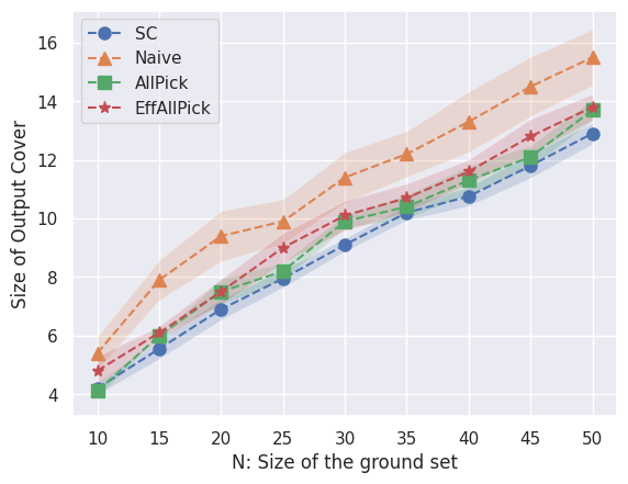
(a) Output size

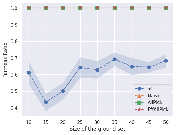
(b) Fairness

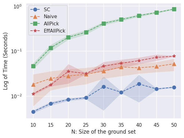
(c) Time

Figure 1. Resume Skills: Comparing (a) the size of output cover, (b) fairness (1 is the max fairness), and (c) running time for various ground set sizes $N$. The results are averaged over 20 samples for each $N$.

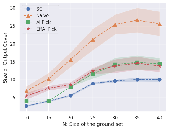
(a) Output size

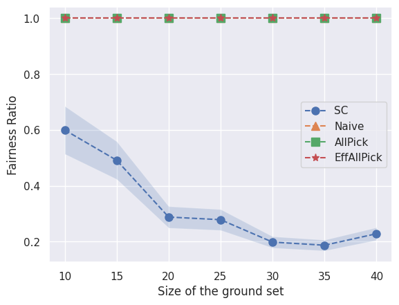
(b) Fairness

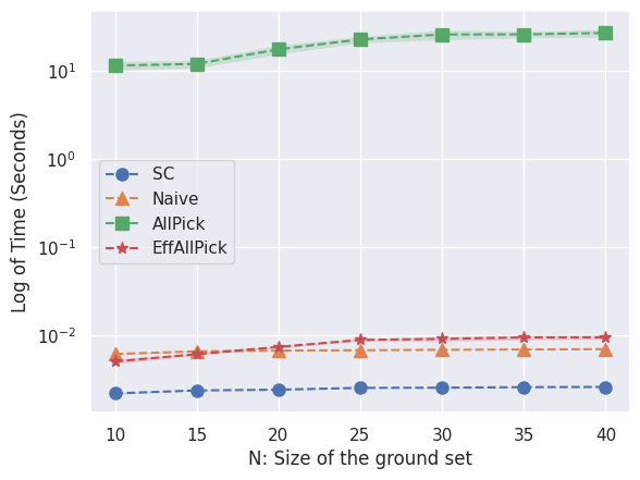
(c) Time

Figure 2. (Non-binary groups): Comparing (a) the size of output cover, (b) fairness, and (c) running time (averaged over 20 samples) for various ground set sizes $N$ for four groups (colors). The probability of colors are $[0.1,0.1,0.2,0.6]$.

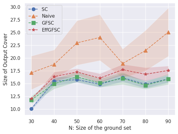
(a) Output size

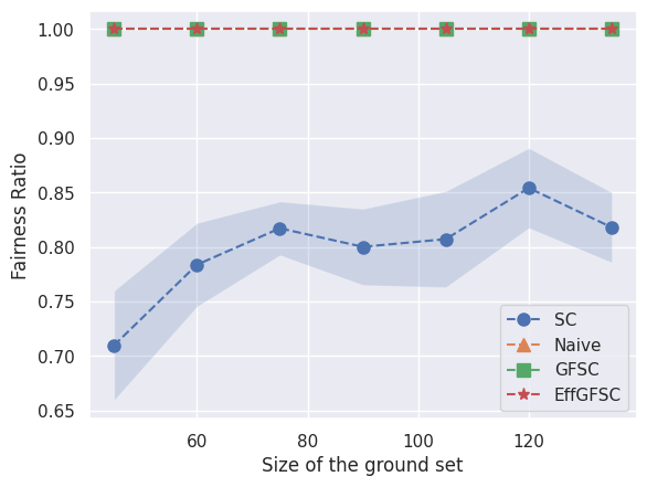
(b) Fairness

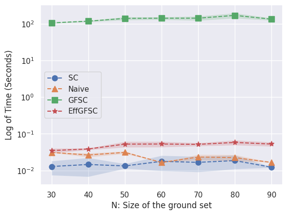
(c) Time

Figure 3. (General Fairness notion): Comparing (a) the size of output cover, (b) fairness based on ratio-parity, and (c) running time (averaged over 20 samples) for various ground set sizes $N$.

Having theoretically analyzed the proposed algorithms, in this section we experimentally evaluate the performance of our algorithms on real and synthetic datasets.

Datasets: Our first set of experiments (§ 7.1 and § 7.2) are motivated by Example 1 (Team of Experts Formation), for which we we use the “Strategeion Resume Skills” dataset. The dataset consists of a 1986 rows as candidates with different skills. The skill of a candidate is shown as 218 binary columns each corresponding to one skill.As an AI Ethics benchmark, the dataset also contains demographic group information, including the (binary) gender. For the second experiments (§ 7.3), we synthesized a dataset, consisting of a number of points as ground set and a family of subsets with different coverage distributions on this ground set. more details about this dataset is provided in Appendix E.

Algorithms: For each of the experiments, we compared the four algorithms: Standard Set Cover (SC), Naive Algorithm (Naive), Greedy Algorithm (AllPick), Efficient or Faster Greedy Algorithm (EffAllPick). We also compared these algorithm with the optimum solution. In order to find the optimum cover, we used the brute-force algorithm for Standard Set Cover (Opt-SC) and a brute-force algorithm for Fair Set Cover (Opt-Fair). These algorithms simply check all possible covers to find the best optimum solution.

Evaluation metrics: We used three metrics for evaluating the algorithms: (a) Output Cover Size, (b) Fairness Ratio, and (c) Running Time. Following our (general) fairness definition in § 3, let the ratio of each group $\mathbf{g}_{h}\in\mathcal{G}$ in the cover $X$ be $R(\mathbf{g}_{h})=\frac{1}{f_{h}}\big{|}\{X\cap\mathcal{S}_{h}\}\big{|}$. Then, the Fairness ratio is computed as

$$\text{Fairness Ratio}=\frac{\min_{\mathbf{g}_{h}\in\mathcal{G}}R(\mathbf{g}_{h})}{\max_{\mathbf{g}_{h}\in\mathcal{G}}R(\mathbf{g}_{h})}$$

This formula for count-parity, for example, computes the least common group size divided by the most common group size in the output cover of an algorithm. A fair algorithm with zero unfairness should return a fairness ratio of 1, while the smaller the fairness ratio, the more unfair the algorithm.

All implementations have been run on a server with 24 core CPU and 128 GB memory with Ubuntu 18 as the OS.

7.1. Validation

We begin our experiments by validating the problem we study. To do so, we used the Resume Skills dataset. Using all of its 1986 rows, we sampled different set of skills $N$ varying from 10 to 20 out of all 218 available skills as the ground set. We run the brute-force algorithms opt-SC and opt-FSC to find the optimal solutions for the set cover and the fair set cover, respectively. Next, we used the greedy algorithm for set cover and EffAllPick for finding the approximate fair set cover. The results are shown in the following table.

Algorithm	Avg. Fairness Ratio	Avg. Cover Size
Opt-SC	0.48	3.32
Greedy-SC	0.55	3.42
Opt-FSC	1.00	3.75
EffAllPick	1.00	3.90

First, we observe that, both optimal and approximation solutions for set cover were significantly unfair, as the presence of women in the cover was only around half of the men. This verifies that without considering fairness, set cover can cause major biases. On the other hand, formulating the problem as fair set cover, both the optimal and the approximation algorithms have zero unfairness. Second, comparing the average cover size for Opt-SC and Opt-FSC, one can verify a negligible price of fairness as the avg. cover size increased by only 0.43 (less than half a set). Last but not least, even though EffAllPick has a $\log(n)$ approximation ratio, in practice its cover size is close to optimal, since its avg. cover size was only 0.15 sets more than the optimal (Opt-FSC).

7.2. Resume Skills

In this experiment, we run experiments of team of experts formation, using the Resume Skills dataset on various settings, while using gender to specify the demographic groups male and female. Let $N$ denote the size of the ground set (i.e., the skill sets to cover). For each $N\in\{15,20,\cdots,50\}$, we randomly selected 20 different samples from these 218 different skills. The goal is to find a fair and minimal set of candidates that cover the ground set. The results, aggregated (average) on all 20 samples, are presented in Fig. 1:

Size of the output cover

From Fig. 1(a), while the output size of the Naive Algorithm is noticeably larger than the greedy set cover (SC), the output sizes for AllPick and EffAllPick algorithms are very close to SC, as the error bars of the three algorithms highly overlap. Also, it is worth to note that, despite the fact that EffAllPick has a slightly worse approximation ratio than AllPick, in practice, the two algorithms performed near-identical.

Fairness Ratio

As one can see in Fig. 1(b), our algorithms guarantee a fairness ratio of 1 but the standard greedy set cover algorithm returned significantly unfair outputs in all cases, all having a fairness ratio less than 0.8.

The Running Time

From Fig. 1(c), we can see that the AllPick Algorithm takes a significantly higher time to find a fair cover. It’s because its time complexity is exponential to the number of colors. On the other hand, using the $\mathsf{LP}$ and Randomized Rounding in EffAllPick significantly reduces this running time.

7.3. Extended results

For these experiments, we use our synthetic data (Appendix E).

7.3.1. Non-binary Demographic Groups

Fig. 2 presents the results for the non-binary setting with four demographic groups. The results are generally consistent with the ones for binary groups (Fig. 1). Moreover, one can see (a) a larger gap between Naive and other algorithms in Fig. 1(a), as a result of its approximation ratio being dependant on $k$ (number of colors), and (b) a larger gap in the running time of AllPick with other algorithms in Fig. 1(c), due to its exponential time complexity to $k$.

7.3.2. Generalized Fair Set Cover

We use ratio-parity as the notion of fairness in this experiment. that is, we want to maintain the original ratio of red and blue sets (0.66 and 0.34) in each selected cover. We compare the four algorithms: standard Greedy Set Cover (SC), Greedy Generalized Fair Set Cover (GFSC), the faster algorithm for Generalized Fair Set Cover (EffGFSC), and the Naive Algorithm (Naive). The Naive Algorithm starts by running SC, which gives an unfair cover. It then balances the color ratios by adding arbitrary sets from other colors (the same approach as the FSC, but here we want to maintain ratios $f_{h}$ for all colors). The results are provided in Fig. 3. As we can see in Fig. 3(a), the output of SC and GFSC were near-identical in all settings. The output cover size of EffGFSC slightly larger but still very close to SC and GFSC. Similar to the previous experiments, Fig. 3(c) confirms that while vanila set cover is not fair, all of out algorithms achieved zero unfairness in all cases. From Fig. 3(c), there is a major gap in the running time of GFSC v.s. other algorithms. However, EffGFSC resolved the issue and significantly reduced the run time.

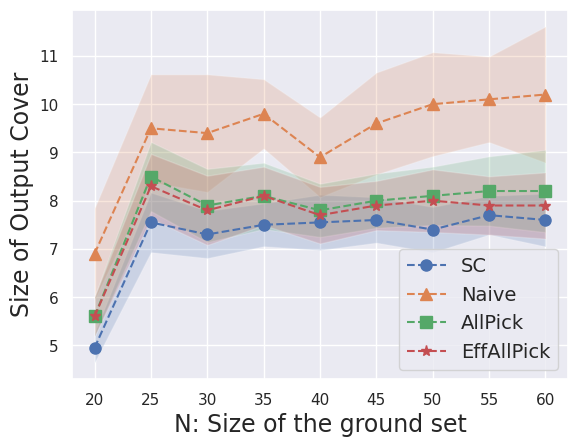
(a) Normal distribution

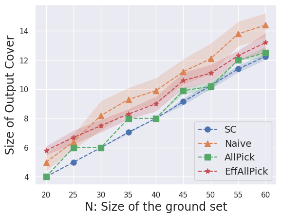
(b) Uniform distribution

Figure 4. Cover sizes for different set coverage distributions.

7.3.3. Set Coverage Distributions

Finally, we conclude our experiments by comparing two cases for set coverage distributions, where in one the sets are uniformly covering the ground set and in the other the coverage of the sets follow a normal distribution with a small standard deviation. In the second case, most of the points in the middle of the ground set (their associated number is close to N / 2) are covered with more sets rather than other points. In Fig 4(a) we can see the size of output cover for these two cases. When the points are not covered uniformly with sets (which is the case in real-world scenarios), the size of the output cover of Naive and EffAllPick algorithms differ significantly. However, in the uniform case, they get close to each other.

8. Related Work

Algorithmic fairness has received a lot of attention in the last few years. However, most of the recent work focuses on the intersection of fairness and Machine Learning  (Barocas et al., 2023)  (Mehrabi et al., 2021).

Despite its importance, limited work has been done on algorithmic fairness in the context of combinatorial problems (Wang et al., 2022). Satisfying fairness constraints while optimizing sub-modular functions is studied in (Wang et al., 2022). Further examples include satisfying fairness in Coverage Maximization problems  (Asudeh et al., 2023; Bandyapadhyay et al., 2021) and Facility Locations (Jung et al., 2019). In this body of work, the focus is on defining fairness on the point set (ground set). In other words, they assume the points belong to different demographic groups. In contrast, in this work, we define fairness on the family of sets. Note that, unlike max coverage, in set cover all points are covered, hence defining fairness on points is irrelevant. Fairness is also studied in problems like Matching (García-Soriano and Bonchi, 2020; Esmaeili et al., 2023), Resource Allocation (Mashiat et al., 2022), Ranking (Asudeh et al., 2019; Zehlike et al., 2017), Queue Systems (Demers et al., 1989), and Clustering (Makarychev and Vakilian, 2021; Thejaswi et al., 2021).

There has been recent work studying fairness in the Hitting Set problem (Inamdar et al., 2023). Although hitting set is the dual of the set cover problem, the definition of fairness used is different from ours. We define and guarantee perfect fairness based on demographic parity (count and ratio parity). In other words, we require an exact equality (e.g., equality of count equality or exact color ratio) between demographic groups. By contrast, in  (Inamdar et al., 2023), a hitting set is defined to be fair if does not contain many points from a color. They have upper bounds on the number of points (equivalent to the subsets in the set cover problem) that can be picked from any particular color (demographic group). Furthermore, they design exact (fixed-parameter) algorithms with running time exponential in $k$ and/or exponential on maximum number of sets that an element belongs to.

9. Conclusion

Set cover has an extended scope for solving real-world problems with societal impact. Therefore, in this paper we revisited this problem through the lens of fairness. We adopted the group fairness notion of demographic parity, and proposed a general formulation that extends to various cases such as count-parity and ratio-parity for binary and non-binary demographic groups. We formulated set cover and weighted set cover under fairness constraint and studied the problem (and approximation) hardness. For each setting, we proposed approximation algorithms that (a) always guarantee fairness, (b) have (almost) the same approximation-ratio and similar time complexity with the the greedy algorithm for set cover (without fairness). Besides theoretical guarantees, our experiments on real and synthetic data across different settings demonstrated the high performance of our algorithms.

Appendix A Application Demonstration (Extension)

Regret-minimizing sets for recommendation

Given a family of preference functions, a minimal subset of data that contains at least one object from the top-$k$ each function is called the (rank) regret-minimizing set (Xie et al., 2020). Regret-minimizing sets are used for recommendation from an overwhelmingly large data set. For example, in a map application (e.g., Google maps), consider a user who is looking for “restaurants”. Instead of highlighting all restaurants, the application can only highlight the regret-minimizing set, knowing that it contains at least a good choice (one of the top-$k$) for any possible user preference. At the same time, the application would like to give an equal exposure to various groups of restaurant owners. This problem also can be formulated with fair set cover, where an object covers a function if it appears in its top-$k$.

Fair Clustering

Clustering is another fundamental problem in Computer Science with many applications in real life such as social network analysis, medical imaging, and anomaly detection (Xu and Wunsch, 2005). There is a lot of work on computing a clustering with small error that satisfies group fairness constraints (Kleindessner et al., 2019; Jones et al., 2020). An instance of the fair clustering problem is usually as follows. We are given a metric space over a set of $n$ elements and a distance function, where each element belongs to a group. We are also given a clustering objective function that measures the error of a clustering. Given a set of $k$ centers, the objective function is used to evaluate the error. The goal is to compute a set of $k$ centers satisfying some fairness constraints that minimize the objective function. For example, in fair $k$-center clustering the goal is to choose a specific fraction of centers from each group such that the maximum distance of an element to its closest center is minimized. Interestingly some of these clustering problems can be modeled as a set cover instance (for example $k$-center clustering). While fair clustering has been studied over different clustering objective functions, such as $k$-center, $k$-median, or $k$-means, there are still significant open problems in the area. In the sum of radii clustering the goal is to choose a set of $k$ balls (where the centers of the balls are elements in the input set) that cover all elements minimizing the sum of radii of the balls. This problem is more useful than the $k$-center clustering (minimize the maximum radius) because it reduces this dissection effect (Hansen and Jaumard, 1997; Monma and Suri, 1989). The standard version of this clustering problem has been thoroughly studied in the literature (Doddi et al., 2000; Charikar and Panigrahy, 2001), however nothing is known for the fair sum of radii clustering, where we want to choose a specific fraction of centers from each group in the final solution. Interestingly, this problem can be mapped to an instance of the fair set cover problem with $n$ elements and $O(n^{2})$ sets: The elements in fair set cover are exactly the elements in the clustering problem. For every element $e$ we construct $O(n)$ balls/sets with center $e$ and radii all possible distances from $e$ to any other element. Each ball/set is assigned a weight which is equal to the radius of the ball. It is not hard to show that any solution of the weighted fair set cover instance is a valid solution for the fair sum of radii clustering and vice versa. Hence, our new algorithm for the fair set cover problem are used to derive the first non-trivial approximation algorithm for the fair sum of radii clustering.

Appendix B Missing proofs from § 3

B.1. Proof of Theorem 3

It is straightforward to show that FSC is $\mathsf{NP}$-complete by a reduction from the standard set cover problem. Given an instance of the set cover problem with $n$ elements $U$ and $\mu$ sets $\mathcal{S}$, for every $\mathbf{g}_{h}\in\mathcal{G}$, we construct $k$ copies of this instance with sets of elements $U_{j}$ and family of sets $\mathcal{S}_{j}$ for $j=1,\ldots,k$. In the construction, we make sure that $U_{j}\cap U_{h}=\emptyset$ for $j\neq h$. For every set $S\in\mathcal{S}_{j}$ we set $\mathbf{g}(S)=\mathbf{g}_{j}$. Finding a fair set cover for $\bigcup U_{j}$ using the sets $\bigcup\mathcal{S}_{j}$ is equivalent to finding a set cover for $U$ using the sets $\mathcal{S}$.

Next, we show that without any assumption, it is $\mathsf{NP}$-Complete to get any non-trivial approximation for the FSC problem.

Assume that there exists an algorithm $\mathcal{A}$ that returns an $f(n)$-approximation algorithm in polynomial time for the FSC problem.

Consider an instance of the standard set cover problem with a set of $n$ elements $U^{\prime}$, a family of $\mu$ sets $\mathcal{S}^{\prime}$ and a parameter $r$. The goal is to decide whether there exists a cover with size at most $r$. For the proof we consider that $r$ is the size of the minimum cover in ($U^{\prime},\mathcal{S}^{\prime}$). We construct an instance of the FSC problem for $\mathcal{G}=\{\mathbf{g}_{1},\mathbf{g}_{2}\}$ as follows. We construct $U_{1}=U^{\prime}$, $\mathcal{S}_{1}=\mathcal{S}^{\prime}$, and we set $\mathbf{g}(e)=\mathbf{g}_{1}$. We also construct a set of $n$ elements $U_{2}$ such that $U_{1}\cap U_{2}=\emptyset$, and a family of $r$ sets $\mathcal{S}_{2}$ such that every $S\in\mathcal{S}_{2}$ contains every element from $U_{2}$ and no element from $U_{1}$. Overall, we constructed the instance of the FSC problem with a set of elements $U=U_{1}\cup U_{2}$ and the family of sets $\mathcal{S}=\mathcal{S}_{1}\cup\mathcal{S}_{2}$. By the construction of $(U,\mathcal{S})$, there is a unique fair cover which consists of the optimum set cover solution in $(U_{1},\mathcal{S}_{1})$ and all sets in $\mathcal{S}_{2}$. Note that this instance of the FSC has only one valid solution that selects all sets in $\mathcal{S}_{2}$, and the $r$ sets from $\mathcal{S}_{1}$ that cover $U_{1}$. Therefore, if an approximation algorithm $\mathcal{A}$ for FSC exists, it must select this solution. Hence, it would solve the Set Cover problem in $(U^{\prime},\mathcal{S}^{\prime})$, which is a contradiction unless $\mathsf{P}=\mathsf{NP}$.

Appendix C Missing algorithms and proofs from § 5

C.1. Naive Algorithm

We first design a naive algorithm for the FWSC, similar to the naive algorithm we proposed for the FSC. We execute the well-known greedy algorithm for the weighted set cover problem in the instance $(U,\mathcal{S})$ without considering the colors of the sets. Let $C$ be the family of sets returned by the greedy algorithm. Then we add arbitrary sets from each color to equalize the number of sets from each color in the final cover. Let $X_{w}$ be the final set we return.

If $\alpha$ is the approximation factor of the greedy algorithm in the weighted set cover, we show that the naive algorithm returns an $\alpha k\Delta$-approximation. Let $C^{*}$ be the optimum solution for the weighted set instance $(U,\mathcal{S})$ and $X_{w}^{*}$ be the optimum solution for the FWSC in the instance $(U,\mathcal{S},w)$. Notice that $w(X_{w}^{*})\geq w(C^{*})$. In the worst case, $C$ contains all the sets from one of the colors $\mathbf{g}_{t}$. As a result, for all other colors, we should add $|C|$ arbitrary sets. For each $h\leq k$ and $h\neq t$, let $A_{h}$ be the family of sets we added to $C$ to form $X_{w}$. Based on the definition, $|A_{h}|=k$ for every $h=1,\ldots,k$, and $X_{w}=C\cup(\bigcup_{h\leq k,h\neq t}A_{j})$. We have:

(1) $$\frac{w(X_{w})}{w(X_{w}^{*})} =\frac{w(C\cup(\bigcup_{h\leq k,h\neq t}A_{j}))}{w(X_{w}^{*})}$$

(2) $$=\frac{w(C)}{w(X_{w}^{*})}+\sum_{h\leq k,h\neq t}\frac{w(A_{j})}{w(X_{w}^{*})}$$

(3) $$\frac{w(C)}{w(C^{*})}+\sum_{h\leq k,h\neq t}\frac{w(A_{j})}{w(C^{*})}$$

(4) $$\leq\alpha+\alpha\sum_{h\leq k,h\neq t}\frac{w(A_{j})}{w(C^{)}}$$

(5) $$\leq\alpha(1+\sum_{h\leq k,h\neq t}\Delta)$$

(6) $$=\alpha(1+(k-1)\Delta)=k\Delta\alpha$$

We know that $\alpha=\ln n+1$, so we have the next result.

Theorem 1.

There exists a $k\Delta(\ln n+1)$-approximation algorithm for the FWSC problem that runs in $O(m\cdot k\cdot n)$ time.

C.2. Proof of Theorem 1

First, it is straightforward to see that $X_{w}$ is a fair cover. The algorithm stops when there is no uncovered element so $X_{w}$ is a cover. In every iteration, we add exactly one set of color $\mathbf{g}_{1}$ and one set of color $\mathbf{g}_{2}$, so $X_{w}$ is a fair cover.

Next, we show that our algorithm computes an $\Delta(\ln n+1)$-approximation solution for the FWSC problem.

Lemma 0.

$w(X_{w})\leq\Delta(\ln n+1)\cdot w(X_{w}^{*})$.

Proof:

The intuition is similar to the proof of Lemma 2, however we write it here for completeness.

If $S_{A},S_{B}\in\mathcal{S}$, let $S_{A,B}=S_{A}\cup S_{B}$. We consider the following instance of the (standard) weighed set cover problem. We define the set $U^{\prime}=U$ and $\mathcal{S}^{\prime}=\{S_{i,j}\mid S_{i}\in\mathcal{S}_{1},S_{j}\in\mathcal{S}_{2}\}$. We also define the weighted function $w^{\prime}:\mathcal{S}^{\prime}\rightarrow\mathbb{R}^{+}$ such that $w^{\prime}(S_{A,B})=w(S_{A})+w(S_{B})$. Let $C^{*}$ be the optimum solution of the weighted set cover instance $(U^{\prime},\mathcal{S}^{\prime},w^{\prime})$. Any fair cover returned by our algorithm can be straightforwardly mapped to a valid weighted set cover for $(U^{\prime},\mathcal{S}^{\prime})$. For example, if our algorithm selects a pair $S_{A},S_{B}$ then it always holds that $S_{A,B}\in\mathcal{S}^{\prime}$, $|(S_{A}\cap S_{B})\cap U|=|S_{A,B}\cap U^{\prime}|$, and $w^{\prime}(S_{A,B})=w(S_{A})+w(S_{B})$. Hence, by definition, we have $w^{\prime}(C^{*})\leq w(X^{*})$.

Recall that the standard greedy algorithm for the weighted set cover problem returns an $(\ln n+1)$-approximation. We show that our algorithm implements a variation of such a greedy algorithm and returns a $\Delta(\ln n+1)$-approximation in the weighted set cover instance $(U^{\prime},\mathcal{S}^{\prime},w^{\prime})$. More specifically, we show that in any iteration, our algorithm chooses a pair of sets $S_{A},S_{B}$ such that the set $\frac{w^{\prime}(S_{A,B})}{|S_{A,B}\cap U^{-}|}$ is a $\Delta$-approximation of the best ratio among the available sets.

At the beginning of an iteration $i$, without loss of generality, assume that our algorithm has selected the pairs $(S_{A_{1}},S_{B_{1}}),\ldots,(S_{A_{i-1}},S_{B_{i-1}})$, so the sets $S_{A_{1},B_{1}},\ldots,S_{A_{i-1},B_{i-1}}$ have been selected for the set cover instance $(U^{\prime},\mathcal{S}^{\prime})$. Let $U^{-}$ be the set of uncovered elements in $U^{\prime}$ at the beginning of the $i$-th iteration. Let $S_{A_{j},B_{j}}$ be the set in $\mathcal{S}^{\prime}$ (at the beginning of the $i$-th iteration) with the minimum $\frac{w^{\prime}(S_{A_{j},B_{j}})}{|S_{A_{j},B_{j}}\cap U^{-}|}$. We consider two cases.

If $S_{A_{j}}\notin\{S_{A_{1}},\ldots,S_{A_{i-1}}\}$ and $S_{B_{j}}\notin\{S_{B_{1}},\ldots,S_{B_{i-1}}\}$, then by definition our greedy algorithm selects the pair $(S_{A_{j}},S_{B_{j}})$ so the set $S_{A_{j},B_{j}}$ is added in the cover of the weighted set cover instance $(U^{\prime},\mathcal{S}^{\prime})$.

Next, consider the second case where $S_{A_{j}}\notin\{S_{A_{1}},\ldots,S_{A_{i-1}}\}$ and $S_{B_{j}}\in\{S_{B_{1}},\ldots,S_{B_{i-1}}\}$ (the proof is equivalent if the set $S_{A_{j}}$ has been selected before). Since there are enough sets from each group, let $S_{B_{h}}$ be a set with color $\mathbf{g}_{2}$ such that $S_{B_{h}}\notin\{S_{B_{1}},\ldots,S_{B_{i-1}}\}$. By definition, we have $|(S_{A_{j}}\cup S_{B_{h}})\cap U^{-}|\geq|(S_{A_{j}}\cup S_{B_{j}})\cap U^{-}|$. Hence, it holds that $w(S_{B_{h}})\geq w(S_{B_{j}})$, otherwise we would have $\frac{w^{\prime}(S_{A_{j},B_{h}})}{|S_{A_{j},B_{h}}\cap U^{-}|}<\frac{w^{\prime}(S_{A_{j},B_{j}})}{|S_{A_{j},B_{j}}\cap U^{-}|}$, which is contradiction. By definition it holds that $\Delta\geq\frac{w(s_{B_{h}})}{w(s_{B_{j}})}$. Our greedy algorithm selects the pair such that $\frac{w(S_{A^{*}})+w(S_{B^{*}})}{|(S_{A^{*}}\cup S_{B^{*}})\cap U^{-}|}$ is minimized, and $S_{A^{*}}\notin\{S_{A_{1}},\ldots,S_{A_{i-1}}\}$, $S_{B^{*}}\notin\{S_{B_{1}},\ldots,S_{B_{i-1}}\}$. Putting everything together, we have,

$$\frac{w^{\prime}(S_{A^{*},B^{*}})}{|S_{A^{*},B^{*}}\cap U^{-}|} =\frac{w(S_{A^{*}})+w(S_{B^{*}})}{|(S_{A^{*}}\cup S_{B^{*}})\cap U^{-}|}\leq\frac{w(S_{A_{j}})+w(S_{B_{h}})}{|(S_{A_{j}}\cup S_{B_{h}})\cap U^{-}|}$$

$$\leq\frac{w(S_{A_{j}})+w(S_{B_{h}})}{|(S_{A_{j}}\cup S_{B_{j}})\cap U^{-}|}\leq\frac{w(S_{A_{j}})+\Delta\cdot w(S_{B_{j}})}{|(S_{A_{j}}\cup S_{B_{j}})\cap U^{-}|}$$

$$\leq\Delta\cdot\frac{w(S_{A_{j}})+w(S_{B_{j}})}{|(S_{A_{j}}\cup S_{B_{j}})\cap U^{-}|}.$$

We conclude that in every iteration, our greedy algorithm computes a set $S_{A,B}$ whose ratio $\frac{w^{\prime}(S_{A,B})}{|S_{A,B}\cap U^{-}|}$ is an $\Delta$-approximation of the best ratio. It is known (Young, 2008) that if a greedy algorithm for the weighted set cover computes a $\beta$-approximation of the best ratio in each iteration, then the algorithm returns a $\beta(\ln n+1)$-approximation. Hence, $w(X_{w})\leq\Delta(\ln n+1)w^{\prime}(C^{*})\leq\Delta(\ln n+1)w(X_{w}^{*})\Leftrightarrow w(X_{w})\leq\Delta(\ln n+1)w(X_{w}^{*})$. $\square$

At the beginning of the algorithm, for every pair of sets we compute the number of elements they cover in $O(m^{2}n)$ time. Each time we cover a new element we update the counters in $O(m^{2})$ time. In total, our algorithm runs in $O(m^{2}n)$ time.

Our algorithm can be extended to $k$ groups, straightforwardly. In each iteration, we find the $k$ sets $S_{A_{1}}\in\mathcal{S}_{1},\ldots,S_{A_{k}}\in\mathcal{S}_{k}$ such that the ratio $\frac{\sum_{1\leq i\leq k}w(S_{A_{i}})}{|\left(\bigcup_{1\leq i\leq k}S_{A_{i}}\right)\cap U^{-}|}$ is minimized. The running time increases to $O(m^{k}n)$.

C.3. Proof of Theorem 2

First, by definition, $C^{(\tau^{*})}$ contains exactly one set from every group $\mathbf{g}_{i}$. Hence $C^{(\tau^{*})}$ always satisfies the fairness requirement. Next, we show the approximation factor and the running time.

We introduce some useful notation. Assume that the optimum solution for the weighted max $k$-color cover instance $(U^{-},\mathcal{S}^{-},w)$ has value $\mathsf{OPT}=\frac{\mathsf{OPT_{w}}}{\tau^{\prime}}$ be the optimum solution covers $\tau^{\prime}$ elements in $U^{-}$ and the sum of weights of all sets in the optimum solution is $\mathsf{OPT}_{w}$. For any $\tau\in[1,n]$, let $\mathsf{OPT}_{\mathsf{LP}}^{(\tau)}=\sum_{S_{i}\in\mathcal{S}^{-}}w(S_{i})x_{i}^{(\tau)}$, i.e., the optimum solution of the $\mathsf{LP}$ with parameter $\tau$. Finally, for $\tau=1,\ldots,n$, let $Z_{i}^{(\tau)}$ be the random variable which is $1$ if $S_{i}$ is selected in the cover (in the last iteration of sampling for the parameter $\tau$), otherwise it is $0$.

Lemma 0.

The expected weight of the family of sets $C^{(\tau)}$ is $\mathsf{OPT}_{\mathsf{LP}}^{(\tau)}$.

Proof:

The expected weight of $C$ is $E[\sum_{i}Z_{i}^{(\tau)}w(S_{i})]=\sum_{i}w(S_{i})E[Z_{i}^{(\tau)}]=\sum_{\mathbf{g}_{h}\in\mathcal{G}}\sum_{S_{i}\in\mathcal{S}^{-}_{h}}w(S_{i})E[Z_{i}^{(\tau)}]=\sum_{\mathbf{g}_{h}\in\mathcal{G}}\sum_{S_{i}\in\mathcal{S}^{-}_{h}}w(S_{i})x_{i}^{(\tau)}=\mathsf{OPT}_{\mathsf{LP}}^{(\tau)}$. $\square$

Lemma 0.

Our algorithm returns an expected $\frac{e}{e-1}$-approximation for the weighted max $k$-color cover problem.

Proof:

$\frac{E[\sum_{i}Z_{i}^{(\tau^{*})}w(S_{i})]}{|C^{(\tau^{*})}\cap U^{-}|}=\frac{\mathsf{OPT}_{\mathsf{LP}}^{(\tau^{*})}}{|C^{(\tau^{*})}\cap U^{-}|}\leq\frac{\mathsf{OPT}_{\mathsf{LP}}^{(\tau^{\prime})}}{|C^{(\tau^{\prime})}\cap U^{-}|}\leq\frac{\mathsf{OPT}_{\mathsf{LP}}^{(\tau^{\prime})}}{(1-\frac{1}{e})\tau^{\prime}}\leq\frac{\mathsf{OPT}_{w}}{(1-\frac{1}{e})\tau^{\prime}}=\frac{e}{e-1}\mathsf{OPT}$. $\square$

Next, we focus on the running time analysis. In total we need to solve $n$ linear programs with $n+k$ variables and $2n+2\mu+1$ constraints, so the running time to execute all the linear programs is $O(n\mathcal{L}(n+k,2n+2\mu+1))$. For each $C^{(\tau)}$ we sample, we compute $|C^{(\tau)}\cap U^{-}|$ in $O(kn)$ time.

It remains to bound the number of times we sample for every $\tau$ to get $|C^{(\tau)}\cap U^{-}|\geq\frac{1}{2}(1-1/e)\tau$. Let $M_{j}^{(\tau)}$ be a random variable which is $1$ if $e_{j}$ is covered, and $0$ otherwise, if sampling according to $x_{i}^{(\tau)}$ is applied.

Lemma 0.

$Pr[\sum_{j}M_{j}^{(\tau)}\geq\frac{1}{2}(1-\frac{1}{e})\tau]\geq\frac{1-1/e}{2n}$.

Proof:

We first compute the expected value $E[\sum_{j}M_{j}^{(\tau)}]$. As we had in the proof of Lemma 6, $Pr[e_{j}\text{ is covered after sampling }]\geq(1-1/e)y_{j}^{(\tau)}$. We have $E[\sum_{e_{j}\in U^{-}}M_{j}^{(\tau)}]=\sum_{e_{j}\in U^{-}}E[M_{j}^{(\tau)}]\geq\sum_{e_{j}\in U^{-}}(1-1/e)y_{j}^{(\tau)}\geq(1-\frac{1}{e})\tau$.

Let $M^{(\tau)}=\sum_{j}M_{j}^{(\tau)}$. Using the reverse Markov inequality, we have $Pr[M^{(\tau)}>\frac{1}{2}(1-1/e)\tau]\geq\frac{E[M^{(\tau)}]-\frac{1}{2}(1-1/e)\tau}{n-\frac{1}{2}(1-1/e)\tau}\\ \geq\frac{(1-1/e)\tau-\frac{1}{2}(1-1/e)\tau}{n-\frac{1}{2}(1-1/e)\tau}=\frac{\frac{1}{2}(1-1/e)\tau}{n-\frac{1}{2}(1-1/e)\tau}\geq\frac{1-1/e}{2n}$. $\square$

Notice that $Pr[\sum_{j}M_{j}^{(\tau)}\geq\frac{1}{2}(1-\frac{1}{e})\tau]$ can be seen as a probability of success in a geometric distribution. In expectation we need $\frac{1}{Pr[\sum_{j}M_{j}^{(\tau)}\geq\frac{1}{2}(1-\frac{1}{e})\tau]}=O(n)$ trials to get a family of sets $C^{(\tau)}$ that cover at least $\frac{1}{2}(1-\frac{1}{e})\tau$ elements in $U^{-}$. Hence, we need to repeat the sampling procedure $O(n)$ times in expectation. Each time that we sample a family of $k$ sets $C^{(\tau)}$, we spend $O(kn)$ time to compute $|C^{(\tau)}\cap U^{-}|$, so for each $\tau$ we spend $O(kn^{2})$ expected time in addition to solving the LP. In total, our algorithm runs in $O(n\mathcal{L}(n+k,2n+2\mu+1)+kn^{3})$ expected time.

C.4. Proof of Theorem 4

Given an instance of the decision version of the Set Cover problem $SC$ for a cover size $l$ ($l=O(n)$, assuming the number of sets is $O(n)$), we map it in polynomial time to an instance of Fair Weighted Set Cover using the function $f(SC,l)$. We conclude that solving $f(SC,l)$ is somehow equivalent to solving the decision version of $SC$ if there is a better approximation ratio.

For an instance of the decision version of Set Cover $SC$ with parameter $l$, we have a ground set $U$ and a family of subsets $\mathcal{F}$. Let $X^{*}$ be the optimum cover $SC$. We say $(SC,l)$ is a ”Yes” instance if $|X^{*}|\leq l$, otherwise, $(SC,l)$ is a ”No” instance. Solving this decision problem is known to be $NP-Complete$.

Define function $f(SC,l)$ that outputs an instance of the Fair Weighted Set Cover problem, given the decision version of $SC$ as an input. Let $U^{\prime}$ be the ground set of $f(SC,l)$ and for some $k\geq 2$ as the number of demographic groups, $\mathcal{F}_{1}$, $\mathcal{F}_{2}$, …, $\mathcal{F}_{k}$ be the family of sets for each demographic group for $f(SC,l)$. The function $w$ assigns a weight to each set in $\bigcup_{h\leq k}\mathcal{F}_{h}$.

Define $U^{\prime}=U\cup\{x\}$ for a new point $x\notin U$. For each $2\leq h\leq k$, define $A_{h}=\{A_{h,i}|A_{h,i}=\{x\},\quad\forall 1\leq i\leq l\}$ and define $B_{h}=\{B_{h_{j}}|B_{h_{j}}=\{x\},j\;\text{is arbitrary large.}\}$ a family of an arbitrary number of sets belonging to color $h$ and only covering $x$ (This will help us to meet the assumption on having enough sets of each color). Define $\mathcal{F}_{1}=\mathcal{F}$ and $\mathcal{F}_{h}=A_{h}\cup B_{h},\quad\forall 2\leq h\leq k$.

Define the set weights as follows:

(7) $$w(S_{t})=\begin{cases}1,&\text{if}\ (\exists h;S_{t}\in A_{h})\;\text{or}\;(S_{t}\in\mathcal{F})\\ \beta,&\text{otherwise}\end{cases}$$

In the above $\beta\geq 1$ is an arbitrary value.

Lemma 0.

If the pair $(SC,l)$ is a ”Yes” instance, then $w^{\prime}(Opt)\leq kl$. Where $Opt$ is the optimum cover for the Fair Weighted Set Cover instance $f(SC,l)$ and $w^{\prime}(Opt)=\sum_{S_{t}\in Opt}w(S_{t})$.

Proof:

Assume $(SC,l)$ is a ”Yes” instance, this means $|X^{*}|\leq l$. As a result the $C=X^{*}\cup(\bigcup_{2\leq h\leq k}A_{h})$ is a fair cover for $U^{\prime}$. Because $U$ is covered by $X^{*}$ and $x\in U^{\prime}$ is covered by $A_{h,i}$s and we have $l$ sets from each color family $\mathcal{F}_{h}$. As a result:

(8) $$w^{\prime}(Opt)\leq w^{\prime}(C)=kl$$

$\square$

Lemma 0.

If the pair $(SC,l)$ is a ”No” instance, then $w^{\prime}(Opt)\geq(\beta+l)(k-1)+l+1$.

Proof:

When $(SC,l)$ is a ”No” instance, this means that we cannot cover $U$ with at most $l$ sets of $\mathcal{F}$. If $Opt$ contains more than $l$ sets of $\mathcal{F}_{1}$, then $B_{h}\cap Opt$ is not empty for some $h$, because $Opt$ is fair and has an equal number of sets from each color. In addition, the sets inside $B_{h}$ do not cover any part of $U$, so we should have at least $l+1$ sets from each color. This means we have at least one set with weight $\beta$ from each color $h\geq 2$. As a result, we have at least $\beta+l$ sum of weights from all colors $h\geq 2$ and at least $l+1$ sum of weights from $\mathcal{F}_{1}$. $\square$

Now assume there is an $\alpha$-approximation algorithm $\mathcal{A}$ for the Fair Weighted Set Cover. For a pair $(SC,l)$, define $C$ to be the output cover of algorithm $\mathcal{A}$.

• If $(SC,l)$ is a ”Yes” instance, $w^{\prime}(C)\leq kl\alpha$.

• If $(SC,l)$ is a ”No” instance, $w^{\prime}(C)\geq(\beta+l)(k-1)+l+1$.

If $\alpha<\frac{(\beta+l)(k-1)+l+1}{kl}$, then based on the value of $w^{\prime}(C)$ one can decide whether $(SC,l)$ is a ”Yes” instance or not. This means an $NP-Complete$ problem is solved in polynomial time. Which is not possible if $P\neq NP$. As a result, $\alpha=\Omega(\frac{\beta}{l}+1)=\Omega(\frac{\Delta}{l}+1)$. Remember that $l=O(n)$, so $\alpha=\Omega(\frac{\Delta}{n}+1)$ for any $\Delta$ and $n$.

Appendix D Missing algorithms and proofs from § 6

As a pre-processing step, our algorithm computes $p_{h}$ for each $\mathbf{g}_{h}$ as follows. Recall that each $f_{h}$ is rational. Without loss of generality, we can assume that each $f_{h}$ is represented in its simplest form. Let $p$ represent the least common multiple (LCM) of the denominators within the set of fractions ${f_{1},\ldots,f_{h}}$. Using standard techniques, $p$ can be computed efficiently. Set $p_{h}=f_{h}\cdot p$ for each group $g_{h}\in\mathcal{G}$.
The performance of our algorithm will have a dependence on $p$. Hence, it is important to observe that $p$ cannot exceed $|\mathcal{S}|=\mu$. This is because in order to satisfy the given fractional constraints, the size of any cover must be at least $p$. However, if $p>\mu$, then this implies the given instance cannot admit such a fractional cover.

In this section, we need the assumption that every group $\mathbf{g}_{h}\in\mathcal{G}$ contain at least $\Omega(\log n)f_{h}|X^{*}|$ sets. For simplicity, we also assume that every group contains the same number of sets, denoted by $m$.

D.1. Greedy Algorithm

The greedy algorithm for the generalized FSC is similar to the greedy algorithm from § 4.2. Instead of choosing one set from each color, in each iteration, we choose a family $C$ of $p$ sets such that, i) $C$ contains $p_{h}$ sets from group $\mathbf{g}_{h}$, and ii) $C$ covers the most uncovered elements in $U$. The proof of Lemma 2 can be applied straightforwardly to the generalized FSC, getting the same approximation guarantee. In terms of the running time, in each iteration we visit $O(\prod_{h}m^{p_{h}})=O(m^{p})$ families of $p$ sets. We conclude to the next theorem.

Theorem 1.

There exists an $(\ln n+1)$-approximation algorithm for the Generalized FSC problem that runs in $O(m^{p}n)$ time.

D.2. Faster Algorithm

In order to make the above algorithm faster, we use a generalized version of the randomized rounding introduced for the FSC. We define the next Integer Program. The only difference with the IP in § 4.3 is that for every group $\mathbf{g}_{h}$, we should satisfy $\sum_{i:S_{i}\in\mathcal{S}^{-}_{h}}x_{i}=p_{h}$ instead of $\sum_{i:S_{i}\in\mathcal{S}^{-}_{h}}x_{i}=1$.

(9) $$\max\sum_{j}y_{j}$$

(10) $$\sum_{i:S_{i}\in\mathcal{S}^{-}_{h}}x_{i} =p_{h},\quad\forall\mathbf{g}_{h}\in\mathcal{G}$$

(11) $$\sum_{i:e_{j}\in S_{i}}x_{i} \geq y_{j},\quad\forall e_{j}\in U^{-}$$

(12) $$x_{i} \in\{0,1\},\quad\forall S_{i}\in\mathcal{S}^{-}$$

(13) $$y_{j} \in\{0,1\},\quad\forall e_{j}\in U^{-}$$

We then replace the integer variables to continuous, as following, and use a polynomial time LP solver to compute the solution of the LP relaxation.

(14) $$x_{i} \in[0,1],\quad\forall S_{i}\in\mathcal{S}^{-}$$

(15) $$y_{j} \in[0,1],\quad\forall e_{j}\in U^{-}$$

Let $x_{i}^{*}$ and $y_{j}^{*}$ be the values of variables in the optimum solution. For each color, we normalize the values $x_{i}^{*}$. More specifically, for every color $\mathbf{g}_{h}\in\mathcal{G}$, and every $S_{i}\in\mathcal{S}^{-}_{h}$ we define $z_{i}^{*}=\frac{x^{*}_{i}}{p_{h}}$. For each color $\mathbf{g}_{h}$, we sample uniformly at random $p_{h}$ sets with replacement according to the probabilities $z^{*}_{i}$. Let $C$ be the family of sets we sample.

If for a color $\mathbf{g}_{h}$, the number of distinct sets picked from the sampling procedure is less than $p_{h}$, then we add arbitrary sets from this color in order to have exactly $p_{h}$ sets. Similarly to the proof of Lemma 6, we have,

$$Pr[e_{j} \text{ not covered by a set in }C]\leq\prod_{\mathbf{g}_{h}\in\mathcal{G}}\left(1-\sum_{i:e_{j}\in S_{i},S_{i}\in\mathcal{S}^{-}_{h}}\frac{x_{i}^{*}}{p_{h}}\right)^{p_{h}}$$

$$\leq\prod_{\mathbf{g}_{h}\in\mathcal{G}}\left(\frac{1}{e^{\sum_{i:e_{j}\in S_{i},S_{i}\in\mathcal{S}^{-}_{h}}\frac{x_{i}^{*}}{p_{h}}}}\right)^{p_{h}}=\prod_{\mathbf{g}_{h}\in\mathcal{G}}\frac{1}{e^{\sum_{i:e_{j}\in S_{i},S_{i}\in\mathcal{S}^{-}_{h}}x_{i}^{*}}}$$

$$=\frac{1}{e^{\sum_{\mathbf{g}_{h}\in\mathcal{G}}\sum_{i:e_{j}\in S_{i},S_{i}\in\mathcal{S}^{-}_{h}}x_{i}^{*}}}=\frac{1}{e^{\sum_{i:e_{j}\in S_{i}}x_{i}^{*}}}\leq\frac{1}{e^{y_{j}^{*}}}.$$

Let $Z_{i}$ be a random variable that returns $1$ if $e_{j}\in C$, and $0$ otherwise. Similarly, to Lemma 7, we have,

(16) $$E[\sum_{j}Z_{j}]\geq(1-\frac{1}{e})OPT_{LP}\geq(1-\frac{1}{e})OPT.$$

After solving the LP in $\mathcal{L}(n+k,2n+2m\cdot k)$ time, we sample $p_{h}$ times from each color $\mathbf{g}_{h}$. Overall, we spend $O(\mathcal{L}(n+k\cdot 2n+2m\cdot k)+p)$ time.

The randomized rounding algorithm is executed in every iteration of the greedy algorithm. The greedy algorithm executes $O(m)$ iterations. Using an analysis similar to § 4.3, we bound the expected number of iterations to $O(\frac{|X^{*}|}{p}\log n)$. Following the same arguments as in § 4.3, we conclude with the next theorem.

Theorem 2.

There is an expected $\frac{e}{e-1}(\ln n+1)$-approximation algorithm for the Generalized FSC problem that runs in $O(m(p+\mathcal{L}(n+k,2n+2m\cdot k)))$ time. The same algorithm also runs in $O(\frac{|X^{*}|}{p}\mathcal{L}(n+k,2n+2m\cdot k)\log n)$ expected time.

D.3. Extensions to GFWSC

Using the results in § 5 along with the main arguments in the current section, all our results for the weighted case can be extended to the generalized FSC. Skipping the details, we have the following results.

Theorem 3.

There exists a $\Delta(\ln n+1)$-approximation algorithm for the Generalized FWSC problem that runs in $O(m^{p}n)$ time.

Theorem 4.

There exists an expected $\frac{e}{e-1}\Delta(\ln n+1)$-approximation algorithm for the Generalized FWSC problem that runs in $O(mn\cdot\mathcal{L}(n+k,2n+2m\cdot k+1)+mpn^{3})$ expected time.

Appendix E Synthetic Dataset Details

Our synthetic dataset for Fair Set Cover has been created considering various parameters, number of demographic groups, etc:

• N: The size of the ground set. We used values between 10 to 70.

• M: The number of subsets. This value is drawn from a normal distribution with mean in $\{4,8,16\}$ and the standard deviation of 1.

• K: Size of color set. We used up to 4 different colors (demographic groups).

• Probability Distribution of Colors: The probability of a set belonging to a color. This is a list of size K. We used either uniform probabilities or a probability that shows a huge bias and existence of some minorities.

• Probability of Set Coverage: The probability of each point being covered by a subset. We used normal distribution with mean equal to N / 2 and the standard deviation in $\{2,5,10\}$. We also used the uniform distribution.

References

- (1)
- Asudeh et al. (2023) Abolfazl Asudeh, Tanya Berger-Wolf, Bhaskar DasGupta, and Anastasios Sidiropoulos. 2023. Maximizing coverage while ensuring fairness: A tale of conflicting objectives. Algorithmica 85, 5 (2023), 1287–1331.
- Asudeh et al. (2019) Abolfazl Asudeh, HV Jagadish, Julia Stoyanovich, and Gautam Das. 2019. Designing fair ranking schemes. In Proceedings of the 2019 international conference on management of data. 1259–1276.
- Atkinson et al. (2007) Anthony Atkinson, Alexander Donev, and Randall Tobias. 2007. Optimum experimental designs, with SAS. Vol. 34. OUP Oxford.
- Bandyapadhyay et al. (2021) Sayan Bandyapadhyay, Aritra Banik, and Sujoy Bhore. 2021. On fair covering and hitting problems. In Graph-Theoretic Concepts in Computer Science: 47th International Workshop, WG 2021, Warsaw, Poland, June 23–25, 2021, Revised Selected Papers 47. Springer, 39–51.
- Barocas et al. (2017) Solon Barocas, Moritz Hardt, and Arvind Narayanan. 2017. Fairness in machine learning. Nips tutorial 1 (2017), 2017.
- Barocas et al. (2023) Solon Barocas, Moritz Hardt, and Arvind Narayanan. 2023. Fairness and machine learning: Limitations and opportunities. MIT Press.
- Bashardoust et al. (2023) Ashkan Bashardoust, Sorelle Friedler, Carlos Scheidegger, Blair D Sullivan, and Suresh Venkatasubramanian. 2023. Reducing Access Disparities in Networks using Edge Augmentation. In Proceedings of the 2023 ACM Conference on Fairness, Accountability, and Transparency. 1635–1651.
- Blanco and Gázquez (2023) Víctor Blanco and Ricardo Gázquez. 2023. Fairness in maximal covering location problems. Computers & Operations Research 157 (2023), 106287.
- Charikar and Panigrahy (2001) Moses Charikar and Rina Panigrahy. 2001. Clustering to minimize the sum of cluster diameters. In Proceedings of the thirty-third annual ACM symposium on Theory of computing. 1–10.
- Cho et al. (2012) Dong-Yeon Cho, Yoo-Ah Kim, and Teresa M Przytycka. 2012. Chapter 5: Network biology approach to complex diseases. PLoS computational biology 8, 12 (2012), e1002820.
- Demers et al. (1989) Alan Demers, Srinivasan Keshav, and Scott Shenker. 1989. Analysis and simulation of a fair queueing algorithm. ACM SIGCOMM Computer Communication Review 19, 4 (1989), 1–12.
- Doddi et al. (2000) Srinivas R Doddi, Madhav V Marathe, Sekharipuram S Ravi, David Scot Taylor, and Peter Widmayer. 2000. Approximation algorithms for clustering to minimize the sum of diameters. In Scandinavian Workshop on Algorithm Theory. Springer, 237–250.
- Donahue and Kleinberg (2020) Kate Donahue and Jon Kleinberg. 2020. Fairness and utilization in allocating resources with uncertain demand. In Proceedings of the 2020 conference on fairness, accountability, and transparency. 658–668.
- Esmaeili et al. (2023) Seyed Esmaeili, Sharmila Duppala, Davidson Cheng, Vedant Nanda, Aravind Srinivasan, and John P Dickerson. 2023. Rawlsian fairness in online bipartite matching: Two-sided, group, and individual. In Proceedings of the AAAI Conference on Artificial Intelligence, Vol. 37. 5624–5632.
- García-Soriano and Bonchi (2020) David García-Soriano and Francesco Bonchi. 2020. Fair-by-design matching. Data Mining and Knowledge Discovery 34 (2020), 1291–1335.
- Ge (2010) Xun Ge. 2010. An application of covering approximation spaces on network security. Computers & Mathematics with Applications 60, 5 (2010), 1191–1199.
- Hansen and Jaumard (1997) Pierre Hansen and Brigitte Jaumard. 1997. Cluster analysis and mathematical programming. Mathematical programming 79, 1-3 (1997), 191–215.
- Hirschman et al. (2007) Jocelyn Hirschman, Steven Whitman, and David Ansell. 2007. The black: white disparity in breast cancer mortality: the example of Chicago. Cancer Causes & Control 18 (2007), 323–333.
- Inamdar et al. (2023) Tanmay Inamdar, Lawqueen Kanesh, Madhumita Kundu, Nidhi Purohit, and Saket Saurabh. 2023. Fixed-Parameter Algorithms for Fair Hitting Set Problems. In 48th International Symposium on Mathematical Foundations of Computer Science.
- Jiang et al. (2021) Yanmin Jiang, Xiaole Wu, Bo Chen, and Qiying Hu. 2021. Rawlsian fairness in push and pull supply chains. European Journal of Operational Research 291, 1 (2021), 194–205.
- Jones et al. (2020) Matthew Jones, Huy Nguyen, and Thy Nguyen. 2020. Fair k-centers via maximum matching. In International conference on machine learning. PMLR, 4940–4949.
- Jung et al. (2019) Christopher Jung, Sampath Kannan, and Neil Lutz. 2019. A center in your neighborhood: Fairness in facility location. arXiv preprint arXiv:1908.09041 (2019).
- Kleinberg et al. (2016) Jon Kleinberg, Sendhil Mullainathan, and Manish Raghavan. 2016. Inherent trade-offs in the fair determination of risk scores. arXiv preprint arXiv:1609.05807 (2016).
- Kleindessner et al. (2019) Matthäus Kleindessner, Pranjal Awasthi, and Jamie Morgenstern. 2019. Fair k-center clustering for data summarization. In International Conference on Machine Learning. PMLR, 3448–3457.
- Ma and Zheng (2021) Yuan Ma and Jiping Zheng. 2021. Fair Regret Minimization Queries. In International Conference on Intelligent Data Engineering and Automated Learning. Springer, 511–523.
- Makarychev and Vakilian (2021) Yury Makarychev and Ali Vakilian. 2021. Approximation algorithms for socially fair clustering. In Conference on Learning Theory. PMLR, 3246–3264.
- Marcelle ([n. d.]) Chantelle Marcelle. [n. d.]. Analysis of Influencer Marketing and Social Media Diversity Reflects Visual Bias. chantellemarcelle.com/influencer-marketing-reflects-social-media-diversity-issue/.
- Mashiat et al. (2022) Tasfia Mashiat, Xavier Gitiaux, Huzefa Rangwala, Patrick Fowler, and Sanmay Das. 2022. Trade-offs between group fairness metrics in societal resource allocation. In Proceedings of the 2022 ACM Conference on Fairness, Accountability, and Transparency. 1095–1105.
- Mehrabi et al. (2021) Ninareh Mehrabi, Fred Morstatter, Nripsuta Saxena, Kristina Lerman, and Aram Galstyan. 2021. A survey on bias and fairness in machine learning. ACM computing surveys (CSUR) 54, 6 (2021), 1–35.
- Monma and Suri (1989) Clyde Monma and Subhash Suri. 1989. Partitioning points and graphs to minimize the maximum or the sum of diameters. In Graph Theory, Combinatorics and Applications (Proc. 6th Internat. Conf. Theory Appl. Graphs), Vol. 2. 899–912.
- Pessach and Shmueli (2022) Dana Pessach and Erez Shmueli. 2022. A review on fairness in machine learning. ACM Computing Surveys (CSUR) 55, 3 (2022), 1–44.
- ReVelle et al. (1976) Charles ReVelle, Constantine Toregas, and Louis Falkson. 1976. Applications of the location set-covering problem. Geographical analysis 8, 1 (1976), 65–76.
- Rubin (1973) Jerrold Rubin. 1973. A technique for the solution of massive set covering problems, with application to airline crew scheduling. Transportation Science 7, 1 (1973), 34–48.
- Simon (2009) Mallory Simon. 2009. HP looking into claim webcams can’t see black people. CNN.
- Swift et al. (2022) Ian P Swift, Sana Ebrahimi, Azade Nova, and Abolfazl Asudeh. 2022. Maximizing fair content spread via edge suggestion in social networks. Proceedings of the VLDB Endowment 15, 11 (2022), 2692–2705.
- Thejaswi et al. (2021) Suhas Thejaswi, Bruno Ordozgoiti, and Aristides Gionis. 2021. Diversity-aware k-median: Clustering with fair center representation. In Machine Learning and Knowledge Discovery in Databases. Research Track: European Conference, ECML PKDD 2021, Bilbao, Spain, September 13–17, 2021, Proceedings, Part II 21. Springer, 765–780.
- Townsend (2017) Tess Townsend. 2017. Most engineers are white and so are the faces they use to train software. Recode.
- Tsang et al. (2019) Alan Tsang, Bryan Wilder, Eric Rice, Milind Tambe, and Yair Zick. 2019. Group-fairness in influence maximization. arXiv preprint arXiv:1903.00967 (2019).
- Vemuganti (1998) Rao R Vemuganti. 1998. Applications of set covering, set packing and set partitioning models: A survey. Handbook of Combinatorial Optimization: Volume1–3 (1998), 573–746.
- Vinicky (2022) Amanda Vinicky. 2022. While a Black-Owned Cannabis Dispensary Opens in Chicago, Critics Say State’s Equity Work Still Falling Short. WTTW.
- Wang et al. (2022) Yanhao Wang, Yuchen Li, Francesco Bonchi, and Ying Wang. 2022. Balancing Utility and Fairness in Submodular Maximization (Technical Report). arXiv preprint arXiv:2211.00980 (2022).
- Xie et al. (2020) Min Xie, Raymond Chi-Wing Wong, and Ashwin Lall. 2020. An experimental survey of regret minimization query and variants: bridging the best worlds between top-k query and skyline query. The VLDB Journal 29, 1 (2020), 147–175.
- Xu and Wunsch (2005) Rui Xu and Donald Wunsch. 2005. Survey of clustering algorithms. IEEE Transactions on neural networks 16, 3 (2005), 645–678.
- Young (2008) Neal E Young. 2008. Greedy set-cover algorithms (1974-1979, chvátal, johnson, lovász, stein). Encyclopedia of algorithms (2008), 379–381.
- Zehlike et al. (2017) Meike Zehlike, Francesco Bonchi, Carlos Castillo, Sara Hajian, Mohamed Megahed, and Ricardo Baeza-Yates. 2017. Fa* ir: A fair top-k ranking algorithm. In Proceedings of the 2017 ACM on Conference on Information and Knowledge Management. 1569–1578.