Universal spectra of noisy parameterized quantum circuits

Abstract

Random unitaries are an important resource for quantum information processing. While their universal properties have been thoroughly analyzed, it is not known what happens to these properties when the unitaries are sampled on the present-day noisy intermediate-scale quantum (NISQ) computers. We implement parameterized circuits, which have been proposed as a means to generate random unitaries, on a transmon platform and model these implementations as quantum maps. To retrieve the maps, a machine-learning assisted tomography is used. We find the spectrum of a map to be either an annulus or a disk depending on the circuit depth and detect an annulus-disk transition. By their spectral properties, the retrieved maps appear to be very similar to a recently introduced ensemble of random maps, for which spectral densities can be analytically evaluated.

Effective methods to sample random unitaries [1] are in high demand for quantum cryptography [2, 3], quantum information processing [4], and algorithm design [5]. From a theoretical perspective, it is natural to sample unitaries uniformly over the unitary group [6]. However, sampling these Haar-random unitaries on a quantum computer is impractical, requiring a number of gates that scale exponentially with the number of qubits [7]. To address this challenge, the concept of $t$-design [8] was adapted [9] to devise shallow sampling circuits, thereby reducing the scaling to polynomial [10, 11].

Pseudo-random unitaries can be generated using circuits that consist of alternating layers of random single- and two-qubit operations [12]. Recently, Sim et al. [13] considered a selection of circuit blocks consisting of layers of parameterized single- and two-quibit rotations. Unitaries are generated by concatenating $\ell$ blocks and sampling over the rotation angles of the resulting circuit. By increasing $\ell$, one can quickly achieve an ’expressibility’ (a practical metric for evaluating sampling quality) comparable to finite-size Haar-random sampling [13].

Useful pseudo-random $d$-dimensional unitaries, $U^{\mathrm{PR}}_{d}$, are expected to posses key properties of their Haar-distributed counterparts. From the spectral perspective, this implies that eigenvalues and eigenvectors of $U^{\mathrm{PR}}_{d}$ should exhibit the features of the Circular Unitary Ensemble [1, 12]. In particular, in the limit $d\rightarrow\infty$, the eigenvalues are expected to uniformly cover the unit circle while their two-point correlation function is expected to follow the Wigner distribution for $\beta=2$ [1, 12, 14].

What happens to these spectral features when $U^{\mathrm{PR}}_{d}$ are sampled on a present-day quantum computer? As implementations on NISQ [15] circuits will inevitably be non-unitary, analyzing features of the unitary spectra is no longer possible. The ability to address the above question thus hinges on answering the following one: Being in the NISQ realm, where should we look for potentially universal spectral features?

In this Letter we analyze spectra of three- and four-qubit parameterized circuits, implemented on IBM quantum processors [16], by modelling these implementations as completely-positive trace-preserving (CPTP) maps [17]. We find that, depending on the depth of a circuit, the distribution of the eigenvalues of the corresponding map follows the ’Single Ring’ scenario [18, 19], i.e., it comes either in the form of an annulus or a disc. We show that a recently introduced ensemble of random maps [20] provides a framework for a classification of NISQ parameterized circuits using two quantifiers only, the strength of dissipation and its rank.

Figure 1 outlines our retrieval procedure, highlighting its three main components: parameterization, tomography, and optimization. We begin by explaining the procedure and then present the experimental results.

Parameterization. NISQ implementations of quantum circuits can be modeled as completely-positive trace-preserving quantum (CPTP) maps [also referred to as ”channels” [21], ”operations” [22], and ”processes” [23]]. Some recent works have already attempted to approximate NISQ circuits and individual gates [24, 25, 26] using Liouvillians [27], which yield specific types of CPTP maps [28, 29]. Here we consider the most general type of CPTP maps (which we will henceforth refer to as ”maps”), operating in $d=2^{n}$-dimensional Hilbert space, with $n$ being the number of qubits.

Figure 1: We retrieve map $\mathcal{T}$ approximating a NISQ circuit with the frequencies $f^{(\bf{s},\bf{b})}_{j}$ collected performing tomography with Pauli strings $P_{\bf{s}}$ and $P_{\bf{b}}$. The map is parameterized with complex matrix $G$, while SPAM errors, modeled using corruption matrix $C$ and input density operator $\rho_{0}$, are encoded with matrices $A_{C}$ and $A_{\rho}$. We determine parameter matrices by minimizing the quadratic loss function $L$, which is based on the differences between frequencies and probabilities yielded by the map, Eq. (2). To find matrices $A_{C}$ and $A_{\text{in}}$, we optimize without the circuit, setting $\mathcal{T}=id$ and $P_{\bf{b}}=\{z,z,...,z\}$.

While a one-to-one parameterization of maps has been proposed [30], we find it impractical due to the trace-preservation condition, which imposes nontrivial constraints on parameter values. Instead, we introduce a parametrization based on the Kraus form [21],

$$\mathcal{T}_{r}(\rho;\bm{\theta})=\sum_{s=1}^{r}K_{s}(\bm{\theta})\rho K_{s}(\bm{\theta})^{\dagger},\leavevmode\nobreak\ \sum_{s=1}^{r}K_{s}(\bm{\theta})^{\dagger}K_{s}(\bm{\theta})={\mathchoice{\rm 1\mskip-4.0mul}{\rm 1\mskip-4.0mul}{\rm 1\mskip-4.5mul}{\rm 1\mskip-5.0mul}}_{d},$$ (1)

where $\bm{\theta}$ is the parameter vector, $K_{i}(\bm{\theta})\in\mathbb{C}^{d\times d}$ are Kraus operators and $1\leqslant r\leqslant d^{2}$ is the rank of the map. $r=1$ corresponds to a unitary map, while $r=d^{2}$ represents the maximal number of Kraus operators needed to specify any map for a chosen $d$.

The second identity in Eq. (1) imposes the trace-preservation condition and implies that, by stacking matrix representations of Kraus operators, we get a rectangular $rd\times d$ matrix $Q$ with the isometry condition $QQ^{\dagger}={\mathchoice{\rm 1\mskip-4.0mul}{\rm 1\mskip-4.0mul}{\rm 1\mskip-4.5mul}{\rm 1\mskip-5.0mul}}_{d}$. We parameterize $Q$ using the QR-decomposition of a complex $rd\times d$ matrix $G$, $G=QR$. The decomposition is made unique by demanding that the upper triangular $d\times d$ matrix $R$ has positive diagonal elements [6]. This procedure yields a set of Kraus operators parameterized by $rd^{2}$ complex numbers given by $\{G_{l,n}\}$. The $2d^{2}$ dimensional vector $\bm{\theta}$ of parameters is constructed by stacking the real and imaginary parts of $\{G_{l,n}\}$.

Our parameterization is only surjective due to the unitary freedom [21]. From the machine-learning (ML) perspective, the fact that different vectors $\bm{\theta}$ yield the same set of Kraus operators – and therefore the same map – is not disadvantageous as both the search space and the optimal manifold dimensions are increased. —

Since our retrieval procedure is based on tomography data, we need to account for state preparation and measurement (SPAM) errors. We do this by considering a non-ideal initial density operator $\rho_{0}=A_{\rho}A_{\rho}^{\dagger}/\text{Tr}[A_{\rho}A_{\rho}^{\dagger}]$, parameterized by a complex $d\times d$ matrix $A_{\rho}$. As aforementioned, here the surjective nature of the parameterization is potentially advantageous for the optimization. To account for measurements errors, generic positive operator-valued measure (POVM) sets $\{E_{j}\}_{j=0,\cdots,d-1}$ [21], are conventionally used; see, e.g., Refs. [33, 34, 25, 35]. However, in the present-day qubit transmon platforms, classical readout errors are dominant [32], which correspond to diagonally dominant matrices $\{E_{j}\}$, with the magnitude of off-diagonal elements often falling below the resolution threshold. We find that for $n\geqslant 3$ and typical number of shots, $N_{s}\leqslant 2^{11}$, a full-fledged POVM modeling would be highly inefficient and even detrimental [31] to the accuracy of the description of measurement errors as compared to the ’diagonal’ readout description [32]. Therefore, we replace the POVM set with $d\times d$ stochastic corruption matrix $C$, so that $(E_{j})_{kl}=\delta_{kl}C_{jl}$, which is parameterized by a $d\times d$ real matrix $A_{C}$, $C_{jl}=|(A_{\text{C}})_{jl}|/\sum_{k=1}^{d}|(A_{\text{C}})_{kl}|$. In total, SPAM errors are parameterized by real $3d^{2}$ vector $\bm{\omega}=\{\text{Re}(A_{\rho})_{i,j},\text{Im}(A_{\rho})_{k,l},(A_{\text{C}})_{k,l}\}_{k,l=1,..,d}$.

Tomography. Several schemes have been proposed [36, 37, 38, 23] and experimentally realized (for $n=1,2$) [39, 40, 41] to retrieve maps from measurements. Many of these schemes are based on the state-map duality (Choi-Jamiołkowski isomorphism) [21], thus reducing the problem to a state tomography; some [40, 41, 23] use the idea of compressed sensing [42] which allows to reduce the number of measurements in the case of low-rank maps.

Considering an arbitrary input state and/or measurement basis is infeasible as the preparation of such state would require a dedicated parameterized circuit of growing depth (in the worst case, exponentially in $n$), thus leading to an exacerbation of the original problem. We therefore utilize the idea of the Pauli string - based tomography [23, 25], that uses only product input states, $|{\bm{s}}\rangle=\bigotimes_{i=1}^{n}|s_{i}\rangle$, with each qubit being in one of the six basis eigenstates, $|s_{i}\rangle\in\{|\pm x_{i}\rangle,|\pm y_{i}\rangle,|\pm z_{i}\rangle\}$. The input product state is prepared with a layer of single-qubit rotations; see Fig. 1, panel ”Tomography”. After passing the circuit, qubits are measured in different Pauli bases, $b_{j}\in\{x_{j},y_{j},z_{j}\}$. A single Pauli measurement mode is specified by vector ${\bm{p}}=(\bm{s},\bm{b})$, ${\bm{s}}=\{s_{1},..s_{n}\}$ and ${\bm{b}}=\{b_{1},..b_{n}\}$. The total number of measurement modes is thus $18^{n}$.

While tomography limited to Pauli strings has not been proven to be able to retrieve any map to arbitrary precision [23], in practice, its accuracy is further limited by the number $N_{\text{mode}}$ of measurement modes used, $N_{m}<18^{n}$, and by the number of shots per mode, $N_{s}$, performed to estimate the probability distributions on the binary string outputs. However, as we discuss below, even under these restrictions, the Pauli-string tomography demonstrates the capability to retrieve spectral densities of the test maps with high accuracy.

Optimization. Similar to Ref. [43], we use a quadratic cost function $L(\bm{\theta})=\sum_{\bf{s},\bf{b},j}\left[\hat{p}^{(\bf{s},\bf{b})}_{j}(\bm{\theta})-f^{(\bf{s},\bf{b})}_{j}\right]^{2}$, where $f^{(\bf{s},\bf{b})}_{j}$ is the frequency of the $j$-th binary output obtained in the experiment with Pauli modes $P_{\bf{s}}$ and $P_{\bf{b}}$, and

$$\hat{p}_{j}^{\bf{s,b}}(\bm{\theta})=\sum_{l=1}^{d}C_{jl}\cdot(P_{\bf{b}}\mathcal{T}(P_{\bf{s}}\rho_{\text{\tiny{0}}}P^{{\dagger}}_{\bf{s}};\bm{\theta})P^{{\dagger}}_{\bf{b}})_{ll}$$ (2)

is the probability yielded by the map, Eq. (1), filtered through the corruption matrix. Here $(A)_{lk}$ is the element of operator $A$ expressed in the computation basis.

To search for minima of the cost function, we employ the Adam optimizer version [45] of the steepest-descent method, $\bm{\theta}\leftarrow\bm{\theta}-\mu\nabla_{\bm{\theta}}L(\bm{\theta})$. Note that, unlike the optimization approaches in Refs. [44, 43], we do not need to constrain the search or project its results on a physically meaningful subspace as our parameterization guarantees that any vector $\bm{\theta}$ yields a valid trace-preserving map.

Figure 2: (a) In the experiment we implement $n$-qubit circuits parameterized with $2n\cdot\ell$ angles, where $\ell$ is the circuit depth. Here a circuit for $n=4$ is shown. (b) Inverse average Kullback-Leibler divergence between frequencies obtained with three-qubit circuits, implemented on ibmq_belem, and probabilities yielded by the identity map $id$ and retrieved rank-$r$ maps, $\mathcal{T}_{r}$, plotted against circuit depth $\ell$. Map $\mathcal{T}^{(1)}_{d^{2}}\circ\mathcal{T}^{(2)}_{d^{2}}$ results from concatenating two maps, independently retrieved with two halves of the original circuit.

The optimization is first performed for the SPAM parameter vector $\bm{\omega}$, without the circuit, $\mathcal{T}=id$, and by omitting base rotation before the measurement, $\vec{b}=\{z,z,...,z\}$. After retrieving $\rho_{0}$ and the corruption matrix $C$, we run the optimization to retrieve the map, by finding parameter vector $\bm{\theta}$ that minimizes $L(\bm{\theta})$.

We benchmark the procedure using different maps, including exponents of Liovillians, and an experiment-relevant SPAM error model [31]. Synthetic data sets are generated by performing $N_{s}=2^{10}$ ’shots’ per measurement mode (as in the experiment). Across all tested models, our procedure consistently retrieves maps with spectral supports closely resembling those of the originals.

Figure 3: Eigenvalues $\{\lambda_{j}\},\leavevmode\nobreak\ j=2,...,d^{2}$ of the maps $\mathcal{T}_{d^{2}}$ retrieved with four-qubit parameterized circuits of varying depth $\ell$ implemented on ibmq_belem. The spectra are invariant under the complex conjugation and only the eigenvalues with $\text{Im}\lambda\geqslant 0$ are plotted. The eigenvalues with $\text{Im}\lambda^{\text{DQ}}\leqslant 0$, of the diluted unitaries $\mathcal{DU}_{d}(p,r)$, obtained as spectral approximations of the maps, are shown together with the corresponding $p$ and $r$ values. Radii of the outer, $R_{+}$ and inner, $R_{-}$, circles are given by $R_{\pm}=\sqrt{(1-p)^{2}\pm p^{2}/r}$.

Results. For the experiment, we adapt one of the parameterized circuits considered in Ref. [13]; see Fig. 2(a). It is composed of $\ell$ blocks, each one consisting of two layers of single-qubit rotations, parameterized with $2n$ angles $\{\varphi_{l},\phi_{l}\}$, $l=1,...,n$, and a ladder of cNOT gates. This particular design allows to quickly reach high expressibility values [13] by gradually increasing $\ell$. For example, when limited to a number of samples $\leqslant 10^{5}$ [31], the expressibility of a four-qubit parameterized circuit of depth $\ell\geqslant 4$ is indistinguishable from that obtained with the Haar-random sampling.

We run experiments with parameterized circuits implemented on the IBM transmon platform ibmq_belem [16], with $N_{\text{mode}}=1784$ ($n=3$) and $N_{m}=8704$ ($n=4$) measurement modes respectively and $N_{s}=2^{10}$ shots per mode. Figure 2(b) illustrates the significance of modeling the implemented circuits using maps rather than unitaries. The accuracy of the modeling of three-qubit circuits is quantified as the Kullback-Leibler (KL) divergence $\overline{D}_{KL}$ between the frequencies estimated in the experiment and the probabilities yielded by the retrieved map. From randomly selected $N_{m}=1784$ measurement modes, we allocate $90\%$ for training and the $10\%$ for estimating the average $D_{\text{KL}}$. The KL-divergence is additionally averaged over ten realizations (samples of angles).

Although the optimized unitary map $\mathcal{T}_{r=1}$ scores slightly better than the ideal unitary map of the circuit, $\mathcal{U}_{c}(\cdot)=U_{c}\cdot U_{c}^{\dagger}$, the full-rank map $\mathcal{T}_{d^{2}}$ yields an accuracy improvement of more than an order of magnitude. Independently optimizing maps $T^{(1)/(2)}_{d^{2}}$ for sub-circuits of length $\ell/2$ and concatenating the results, we obtain a map that, while yielding lower accuracy than $\mathcal{T}{d^{2}}$, still demonstrates substantially higher accuracy than the unitary approximation.

Figure 3 presents the spectra $\{\lambda_{j}\},\leavevmode\nobreak\ j=2,...,d^{2}$ (the leading eigenvalue $\lambda_{1}=1$ is not shown) of the retrieved full-rank maps for random four-qubit parameterized circuits of increasing depths (the results for three-quibit circuits are presented in the SM [31]). The eigenvalues are located inside the unit disk thus highlighting a strong non-unitarity character of the maps. Eigenvalues are arranged in an annulus-like spectral distribution whose outer and inner radii diminishing as $\ell$ increases, eventually undergoing an annulus-disc transition.

Figure 4: (a) Outer and inner radii of the diluted unitaries in the limit $d\rightarrow\infty$ (lines) compared to the maximal and minimal eigenvalues $|\lambda_{j}|_{j=2,...,d^{2}}$ (symbols) of the retrieved four-qubit maps. (b) Spectra of the map retrieved for a four-qubit map of the depth $\ell=16$ and of a randomly sampled diluted unitary from the ensemble $\mathcal{DU}_{0.71,23}$. The eigenvalues are superimposed onto the spectral density obtained by sampling over $10^{4}$ diluted unitaries from $\mathcal{DU}_{0.71,23}$. The inset compares histograms of $|\lambda_{j}|$ and $|\lambda^{\text{DU}}_{j}|$.

A similar scenario was recently reported for the ensemble of random maps [20],

$$\mathcal{DU}_{p,r}(\cdot)=pU\cdot U^{\dagger}+(1-p)\sum_{s=1}^{r}K_{s}\cdot K_{s}^{\dagger},$$ (3)

which we henceforth refer to as the diluted unitaries (DU). A DU ensemble is parameterized by the relative strength of the dissipative term, $0<p<1$, and its rank, $r=1,...,d^{2}$. $U$’s are sampled from the ensemble of Haar random unitaries while the Kraus operators $\{K_{s}\}$ are sampled by using rectangular $d\times dr$ Ginibre matrix (as described in the ”Parameterization” section). Because of the close similarity between the spectra retrieved in the experiment and those obtained for DU ensembles, we employ the latter as a tool to describe and analyze how the spectral densities of the NISQ circuits evolve with increasing $\ell$.

To identify ensemble $\mathcal{DU}_{p,r}$ with the spectral support best approximating that of the retrieved map, we minimize the $2$-Wasserstein distance between the Gaussian kernel density estimators of the eigenvalues of the retrieved map and those of a typical member of $\mathcal{DU}_{p,r}$ [31].

It is noteworthy that, although we used a generic full-rank map, Eq. (1), to model the action of the NISQ circuits, the corresponding approximating DUs have ranks substantially lower than $d^{2}$ which, in addition, depend on $\ell$. Thus, together with the dissipation strength $p$, the rank of the approximating DU can be used to label an ensemble of parameterized NISQ circuits of fixed depth $\ell$. The values of $p$ and $r$ for different $\ell$ are presented in Fig. 3 as well as the spectrum of a randomly sampled member of $\mathcal{DU}_{p,r}$.

In the asymptotic limit, $d\to\infty$, the spectral densities of DUs can be evaluated by using free probability theory [46]. In this limit, the inner $R_{-}$ and outer $R_{+}$ radii of the spectral support are given by $R_{\pm}=\sqrt{(1-p)^{2}\pm p^{2}/r}$ [20]. Figure 4(a) presents a comparison of the asymptotic radii as functions of $p$ for different $r$, with the smallest and largest absolute values in the spectrum $\{\lambda_{j}\}_{j=2,...,d^{2}}$ of the retrieved map. The matching is quite accurate, even for a relatively small dimension $d=2^{4}=16$. Figure 4(b) shows that not only the spectral support matches, but even the distribution of the eigenvalues is well reproduced by that of the approximating DU. Note that the eigenvalues displayed in the lower semi-plane of Fig. 4(b) correspond to a random sample from the ensemble $\mathcal{DU}_{0.71,23}$.

Conclusion and outlook. We demonstrated that NISQ parameterized circuits, when modeled as quantum maps, display universal spectral properties. Specifically, their spectral supports, which come in the form of an annulus or a disc, are independent of the particular parameter choices and only depend on the circuit depth.

We found that the Diluted Unitary model [20] is able to accurately reproduce the evolution of the spectral support with the circuit depth [20]. This suggests that the maps retrieved from NISQ parameterized circuits and diluted unitaries are particular manifestations of a broader underlying universality. In Ref. [47], the annulus-disc transition is detected in the spectra of concatenations of unitary and purely dissipative maps. Moreover, this transition is also observed in the spectra of maps obtained by exponentiating Lindbadians with random Hamiltonan and dissipative components [48]. We believe that the annulus-disc scenario can be modeled in the framework of non-Hermitian random matrix theory [49] and can thus be related to the Single-Ring Theorem [18, 19].

We also found evidence that the evolution of multi-qubit states in NISQ circuits is significantly influenced by non-Markovian effects [50, 51]. Specifically, while the concatenation of two maps, each one modeling a half of a NISQ circuit, offers a notably improved approximation of the entire circuit compared to the unitary description (see Fig. 2b), the concatenated map exhibits significantly reduced accuracy compared to the map approximating the whole circuit. Quantifying the degree of non-Markovianity [50, 51] in NISQ circuits is an interesting task, notwithstanding experimental challenges.

Finally, our findings emphasize present-day NISQ computers as versatile platforms for exploring Dissipative Quantum Chaos (DQS). This emerging theory aims, by utilizing the theoretical framework of non-Hermitian random matrix theory [49], to figure out how properties of open quantum evolution, induced by CPTP maps and quantum Liouvillians, are encoded in the spectral features of the latter [52, 53, 54, 55, 56, 58, 20, 24, 59, 47, 60, 61, 62, 63]. In this perspective, the existing NISQ platforms can play a role similar to the role microwave billiards played in the experimental verification of the Hamiltonian Quantum Chaos theory [64].

We thank Karol Życzkowski, Tomaž Prosen, Dariusz Chruściński, and Lucas Sá for useful discussions. We acknowledge the use of IBM Quantum services for this work. This research is supported by Research Council of Norway, project “IKTPLUSS-IKT og digital innovasjon - 333979” (KW and SD) and by FCT-Portugal (PR), as part of the QuantERA II project “DQUANT: A Dissipative Quantum Chaos perspective on Near-Term Quantum Computing” via Grant Agreement No. 101017733. PR acknowledges further support from FCT-Portugal through Grant No. UID/CTM/04540/2020.

Supplemental Material for
“Universal spectra of noisy parameterized quantum circuits”

I The parameterized circuit and its expressibility

For the experiment, we adapted a circuit from Ref. [S1], referred therein as ’Circuit 2’. A circuit block, sketched in Fig. 2a in the main text, consists of two layers of single-qubit parametrized rotations and a ladder-like chain of CNOT gates (we replaced $R_{x}$ rotations in the first layer of the original design with $R_{y}$). The block is parameterized with $2n$ angles, $\{\varphi_{1},...,\varphi_{n},\phi_{1},...,\phi_{n}\}$, where $n$ is the number of qubits.

The expressibility [S1] of the circuit $U_{\ell}(\bm{\psi})$, consisting of $\ell$ blocks and parameterized by $2n\ell$-dimensional vector of angles, $\bm{\psi}$, is defined as the Kullback-Leibler (KL) divergence,

$$\text{Expr}(N_{\text{sample}})=D_{\text{KL}}\bigl{[}p_{\ell}(F;N_{\text{sample}})|p_{\text{Haar}}(F;N_{\text{sample}})\bigr{]},$$ (S1)

between the distribution of the fidelitiy $p_{\ell}(F;N_{\text{sample}})$, $F=\left|\langle\bm{0}|U_{\ell}(\bm{\psi})|\bm{0}\rangle\right|^{2}$, obtained with the circuit by uniformly sampling $N_{\text{sample}}$ times over $2n\ell$ angles, and the distribution corresponding to the Haar random sampling, $p_{\text{Haar}}(F;N_{\text{sample}})$ (note that, in the limit $N_{\text{sample}}\to\infty$, the analytical form of the distribution is known, $p_{\text{Haar}}=(d-1)(1-F)^{d-2}$ [S2]). Finally, as the probability distributions need to be estimated with histograms, there is one more parameter which is the number $N_{\text{bins}}$ of bins per unit interval. We use the same number, $N_{\text{bins}}=75$, as in Ref. [S1].

In Fig. S1, we show the expressibility of the circuit as the function of its depth $\ell$, for two numbers of $N_{\text{sample}}$. Starting from $\ell=4$, the expressibility of the circuit matches the expressiblity of the genuine Haar-random sampling for $N_{\text{sample}}=10^{4}$ and $10^{5}$.

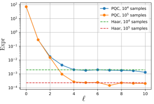
Figure S1: Expressibility, Eq. S1, of the parameterized circuit used in the experiment, as function of the number of concatenated blocks, $\ell$, for two numbers of samples. The number of bins per unit interval is 75.

II POVM set and corruption matrix

We parameterize the POVM set, $\{E_{j}\}$, by using Ginibre matrices $G_{j}=A_{j}+iB_{j}$ ($A_{j},B_{j}\in\mathbb{R}^{d\times d}$),

$$E_{j}=\frac{1}{\sqrt{D}}H_{j}\frac{1}{\sqrt{D}},$$ (S2)

where $H_{j}=G_{j}G_{j}^{\dagger}$, and $D=\sum_{i=1}^{d}{H_{i}}$ is the normalizing matrix.

We restrict the measurement errors to classical read-out errors and introduce corruption matrix $C$, a stochastic matrix which is parameterized in the following way: Let $A_{1}\in\mathbb{R}^{d\times d}$. Then,

$$C_{ij}=\frac{|(A_{1})_{ij}|}{\sum_{k=1}^{d}|(A_{1})_{kj}|}.$$ (S3)

The corruption matrix can be related to the POVM set $\{E_{i}\}$ by setting all the off-diagonal of all $E_{j}$’s to zero and defining elements of the corruption matrix as

$$C_{ik}\coloneqq(E_{i})_{kk}.$$ (S4)

The off-diagonal elements of $E_{j}$ have absolute values substantially lower than diagonal elements. Thus finite-size fluctuations in the estimation of the off-diagonal elements can accumulate, leading to changes comparable to (or even exceeding) those induced by the statistical fluctuations of the diagonal elements. In this scenario, accurate estimation of the non-diagonal elements is statistically challenging and rather useless as the main contribution to errors comes from the diagonal elements. This motivated us to use the corruption matrix instead of a generic POVM. A further advantage is that the former has $\mathcal{O}(d^{2})$ free parameters as opposed to $\mathcal{O}(d^{3})$ of the latter.

By using synthetic benchmarks (as described in the next session), we find that the limitations in the number of measurement modes, $N_{m}$, and shots, $N_{s}$, emerging in the experiment, do not allow us to collect sufficient data to ensure that the retrieved POVMs surpass the corruption matrix in modeling measurement errors. Instead, the POVM approach exhibits inferior performance, making the corruption matrix the preferable option; see Fig. S2.

III Benchmarking

To benchmark the procedures for the retrieval of SPAM models and maps, we generate synthetic data that mimic the experimental situation.

III.1 SPAM Model

We define the synthetic SPAM model as

$$\begin{split}\rho_{in}=c_{1}\left|\bm{0}\right\rangle\left\langle\bm{0}\right|+(1-c_{1})\delta\rho,\\ E^{\text{true}}_{j}=c_{2}\left|\bm{j}\right\rangle\left\langle\bm{j}\right|+(1-c_{2})\delta E_{j}.\end{split}$$ (S5)

Here, $c_{1},c_{2}\in[0,1]$ and $\left|\bm{0}\right\rangle\left\langle\bm{0}\right|$ and $\left|\bm{j}\right\rangle\left\langle\bm{j}\right|$ represent the density operator corresponding to the ideal initial state and projectors on the basis states. We mixed these operators, in the convex way, with randomly sampled quantum states $\delta\rho$, and POVM sets $\delta\{E_{j}\}$, respectively. Using them, we calculate the probabilities $\{p_{j}^{\bm{s}}\}$ over binary string outputs $\{\bm{j}\}$, by applying different Pauli strings to the initial state and ’measuring’ the results with the POVMs,

$$p_{j}^{\bm{s}}=\mathrm{Tr}[E^{\text{true}}_{j}P_{\bm{s}}\rho_{in}P_{\bm{s}}^{\dagger}],$$ (S6)

Finally, we obtain synthetic data, ’frequencies’ $\hat{f}_{j}^{\bm{s}}$, by sampling from the probability distribution, Eq. (S6), $N_{\text{sample}}$ times.

For the benchmarking, we use $c_{1}=0.9$ and $c_{2}=0.8$, to emulate $10\%$ and $20\%$ corruption of the initial state and the classical read-out errors, respectively. We consequently run two optimization procedures, for the corruption matrix and for the POVM set, with the same synthetic data, obtained for $N_{m}=6^{n}$ randomly selected measurement modes and different $N_{\text{sample}}$. The retrieved POVM set $\{E_{j}\}$ is then compared to the ground-truth set $\{E^{\text{true}}_{j}\}$, by calculating the POVM fidelity,

$${\text{Fidelity}}(\{E^{\text{true}}_{j}\},\{E_{j}\})=\frac{1}{d}\sum_{i=1}^{d}{\text{Tr}}[\sqrt{E^{\text{true}}_{j}\cdot E_{j}}]\in[0,1].$$ (S7)

Figure S2 presents the results of the test.

When optimizing SPAM error models, we observed that multiple choices of $\rho_{0}$ and ${E_{i}}$ (or $C$) result in local minima of the cost function which yield the same values for the latter. This degeneracies arise from permutations of the computational basis an d each set of operators corresponds to a physically distinct SPAM error model. The problem can be resolved by identifying the relevant solution as the one that has $\rho_{in}$ closest to the ideal initial state, $\left|\bm{0}\right\rangle\left\langle\bm{0}\right|$, the POVM elements closest to the projectors, and the corruption matrix located near the identity ${\mathchoice{\rm 1\mskip-4.0mul}{\rm 1\mskip-4.0mul}{\rm 1\mskip-4.5mul}{\rm 1\mskip-5.0mul}}_{d}$.

When optimizing SPAM error models, we noted that multiple choices of $\rho_{0}$ and $\{E_{i}\}$ (or $C$) lead to equivalent local minima of the cost function. This degeneracy of the SPAM models stems from permutations of the computational basis. Different choices of operators correspond to physically distinct SPAM error models, with only one of them being reasonable. The degeneracy can be removed by realizing that this reasonable solution corresponds to $\rho_{in}$ that is the closest one to the ideal initial state, $\left|\bm{0}\right\rangle\left\langle\bm{0}\right|$, POVM elements that are closest to the projectors, and the corruption matrix located in the vicinity of the identity ${\mathchoice{\rm 1\mskip-4.0mul}{\rm 1\mskip-4.0mul}{\rm 1\mskip-4.5mul}{\rm 1\mskip-5.0mul}}_{d}$.

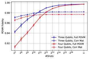
Figure S2: POVM Fidelity, Eq. (S7), between ground truth and retrieved SPAM models fitted to synthetic data, as function of the number of shots. Both POVM sets (solid line) and a corruption matrices (dashed line) were optimized.

III.2 Synthetic data from CPTP maps

We benchmark our retrieval procedure using synthetic data generated with various maps and the SPAM model (describe in the previous section), under condition of fixed number of samples, $N_{\text{sample}}=2^{10}$ (the number of shots per measuring mode used in the experiment).

Here we present the results obtained with maps that are constructed by exponentiating different Lindbladians, $\Phi=e^{\beta\mathcal{L}}$, where $\beta\geq 0$ determines the ’strength’ of the map (e.g., $\beta=0$ yields the identity map).

The Lindbladians are constructed by combining random Hamiltonians and random dissipative parts. Specifically, Hamiltonians are sampled as GUE matrices, $H=\frac{G_{H}+G_{H}^{\dagger}}{2}$, where $G_{H}\in\mathbb{C}^{d\times d}$. The dissipative part is specified with a Choi matrix $\phi=G_{\phi}G_{\phi}^{\dagger}$, where $G_{\phi}\in\mathbb{C}^{d^{2}\times r}$ and $r$ is the rank. We define the Lindbladian as a matrix,

$$\mathcal{L}=-i\alpha(I\otimes H-H^{T}\otimes I)+\phi-\frac{1}{2}({\text{Tr}}_{B}(\phi)^{T}\otimes I-I\otimes{\text{Tr}}_{B}(\phi)),$$ (S8)

where $\alpha\geq 0$ determines relative contribution of the Hamiltonian (unitary) component on the overall dynamics.

The probability distribution $p_{j}^{\bm{s},\bm{b}}$ is obtained by applying Pauli string $P_{\bm{s}}$ to the initial state $\rho_{in}$, which is then acted upon with the map $\Phi$, rotated to the measurement basis with Pauli string $P_{\bm{b}}$ and finally ’measured’ by using POVM set $\{E_{j}\}$,

$$\begin{split}\rho^{\bm{s}}=\Phi(P_{\bm{s}}\rho_{in}P_{\bm{s}}^{\dagger})\\ p_{j}^{(\bm{s},\bm{b})}=\mathrm{Tr}[E_{j}P_{\bm{b}}\rho^{\bm{s}}P_{\bm{b}}^{\dagger}].\end{split}$$ (S9)

Finally, we derive synthetic data, ’frequencies’ $f_{j}^{\bm{s},\bm{b}}$, by sampling from $p_{j}^{\bm{s},\bm{b}}$ $N_{\text{shot}}$ times. We used the same number of randomly selected Pauli modes $(\bm{s},\bm{b})$ as in the experiment, $N_{m}=1784$ (three qubits) and $N_{m}=8704$ (four qubits).

In Figure S3, we compare the retrieved spectra (orange dots) with the spectra of the original maps (blue dots). Although the accuracy in matching eigenvalues as a finite set of points on the plane leaves room for further improvement, the procedure is able to capture the spectral support and spectral density quite accurately.

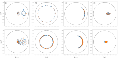
Figure S3: Spectra of original maps (blue dots), Eqs. (S5-S6), and of the retrieved maps (orange dots) for $n=3$ (upper panel) and $n=4$ (lower panel). Parameters of the map are (a) $\alpha=1$, $\beta=0.1$, $r=1$, (b) $\alpha=10^{4}$, $\beta=10^{-3}$, $r=16$, (c) $\alpha=10^{2}$, $\beta=10^{-3}$, $r=16$, (d) $\alpha=1$, $\beta=10^{-2}$, $r=8$.

III.3 Spectral Fitting

Diluted Unitaries (DU) [S3] constitute an ensemble of random maps,

$$T_{\text{Diluted}}(\rho)=(1-p)U\rho U^{\dagger}+p\sum_{j=1}^{r}K_{j}\rho K_{j}^{\dagger},$$ (S10)

where $U$ is a Haar-random unitary and $\{K_{j}\}_{j=1,2,...,r}$ is a set of random Kraus operators of given rank $r$. The parameter $p$ weights the relative strength of the dissipative part.

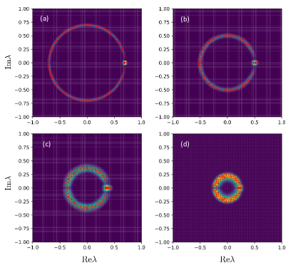
Figure S4: Histograms of the spectra $\{\lambda_{j}\},\leavevmode\nobreak\ j=2,...,d^{2}$ of the maps $\mathcal{T}_{d^{2}}$ retrieved with three-qubit parameterized circuits of varying depth $\ell$, implemented on ibmq_belem. For each value of $\ell$, we retrieved spectra of ten circuits, obtained by randomly sampling over the rotation angles. Each plot displays a two-dimensional histogram obtained with $10(2^{6}-1)=630$ eigenvalues (eigenvalue $1$ is not included). The red dots represent eigenvalues of a diluted unitary with $p$ and $r$ obtained by minimizing the spectral distance to one (randomly sampled) diluted unitary and one (randomly chosen) realization of the parameterized circuit.

We aim to determine values of $p$ and $r$ such that the spectrum of the diluted unitary maximally overlaps with the spectrum of a given map. To measure this overlap, we introduce the spectral distance (SD) defined in the following way: Given two spectra, $S^{(a)}=\{\lambda^{(a)}_{1},\lambda^{(a)}_{2},\cdots,\lambda^{(a)}_{d^{2}}\}$ and $S^{(b)}=\{\lambda^{(b)}_{1},\lambda^{(b)}_{2},\cdots,\lambda^{(b)}_{d^{2}}\}$, the spectral distance (SD) is calculated as

$$\text{SD}(S^{(a)},S^{(b)})=\int[p(\lambda;S^{(a)},\sigma)-p(\lambda;S^{(b)},\sigma)]^{2}d\lambda,$$ (S11)

where $p(\lambda;S^{(a)},\sigma)$ is a kernel density estimation over the spectrum $S^{(a)}$, using a ywo-dimensional Gaussian kernel of width $\sigma$. It is given by the sum

$$p(\lambda;S^{(a)},\sigma)=\frac{1}{d^{2}}\sum_{i=1}^{d^{2}}\mathcal{N}(\lambda;\lambda^{(a)}_{i},\sigma).$$ (S12)

The integral in Eq. S11 can be computed analytically, resulting in the expression

$$\text{SD}(S^{(a)},S^{(b)})=\frac{1}{d^{4}}\sum_{i=1,j=1}^{d^{2}}\left[\mathcal{N}(\lambda^{(a)}_{i};\lambda^{(a)}_{j},\sigma)+\mathcal{N}(\lambda^{(b)}_{i};\lambda^{(b)}_{j},\sigma)-2\mathcal{N}(\lambda^{(a)}_{i};\lambda^{(b)}_{j},\sigma)\right].$$ (S13)

To compute the spectral distance (SD) between the spectrum $S^{(a)}$ of the map and the spectrum $S^{(b)}$ of the diluted unitary (DU), we first need to specify $\sigma$. We choose this parameter to be equal to the average nearest-neighbor distance of the eigenvalues of the map. By minimizing the SD, we observe that weak variations of $\sigma$ around this value result in near the same values of $p$ and $r$, thus confirming that the average nearest-neighbor distance is a reasonable choice for $\sigma$.

IV Results for parameterized circuit with three qubits

Figure S4, similar to Fig.3 in the main text, presents the spectra retrieved from experimental data collected with three-qubit parameterized circuits of varying depth $\ell$, implemented on ibm_belem. For each depth value, we sampled ten random sets of angles and retrieved the ten corresponding spectra. We calculated two-dimensional histograms using $10(2^{3\cdot 2}-1)=630$ eigenvalues for each value of $\ell$. The histograms are plotted together with the spectra of diluted unitaries with $p$ and $r$ values obtained by minimizing the spectral distance to one (out of ten) of the circuit realizations.

References

[S1] S. Sim, P. D. Johnson, and A. Aspuru-Guzik, Expressibility and entangling capability of parameterized quantum circuits for hybrid quantum-classical algorithms, Adv. Quantum Technol.  2, 1900070 (2019).

[S2] K. Życzkowski and H. J. Sommers, Average fidelity between random quantum states, J. Phys. A 71, 032313 (2005).

[S3] L. Sá, P. Ribeiro, T. Can, and T. Prosen, Spectral transitions and universal steady states in random Kraus maps and circuits, Phys. Rev. B 174, 134310 (2020).

References

- [1] K. Życzkowski and M. Kuś, Random unitary matrices, J. Phys. A: Math. Gen. 2 4235 (1994).
- [2] S. Pirandola et al., Advances in quantum cryptography, Adv. Opt. Photon. 12, 1012 (2020).
- [3] C. Portmann and R. Renner, Security in quantum cryptography, Rev. Mod. Phys. 94, 025008 (2022).
- [4] A. Abeyesinghe, I. Devetak, P. Hayden, and A. Winter, The mother of all protocols: restructuring quantum information’s family tree, Proc. R. Soc. A. 465, 2537 (2009).
- [5] A. M. Childs and W. van Dam, Quantum algorithms for algebraic problems, Rev. Mod. Phys. 82, 1 (2010).
- [6] F. Mezzadri, How to generate random matrices from the classical compact groups, Not. Am. Math. Soc. 54, 592 (2007).
- [7] E. Knill, Approximation by quantum circuits, LANL report LAUR-95-2225 (1995); arXiv:9508.8006.
- [8] P. Delsarte, J. M. Goethals, and J. J. Seidel, Spherical codes and designs, Geom. Dedicata 6, 363 (1977).
- [9] D. Gross, K. Audenaert, and J. Eisert, Evenly distributed unitaries: on the structure of unitary designs, J. Math. Phys. 48, 052104 (2007).
- [10] F. Brandao, A.W. Harrow, and M. Horodecki, Local random quantum circuits are approximate polynomial-designs, Commun. Math. Phys. 346, 397 (2016).
- [11] J. Haferkamp, P. Faist, N. B. T. Kothakonda, J. Eisert, and N. Y. Halpern, Linear growth of quantum circuit complexity, Nat. Phys. 18, 528 (2022).
- [12] J. Emerson, Y. S. Weinstein, M. Saraceno, S. Lloyd, and D. G. Cory, Pseudo-random unitary operators for quantum information processing, Science 302, 2098 (2003).
- [13] S. Sim, P. D. Johnson, and A. Aspuru-Guzik, Expressibility and entangling capability of parameterized quantum circuits for hybrid quantum-classical algorithms, Adv. Quantum Technol. 2, 1900070 (2019).
- [14] M. Poźniak, K. Życzkowski, and M. Kuś, Composed ensembles of random unitary matrices, J. Phys. A 31, 1059 (1998).
- [15] J. Preskill, Quantum Computing in the NISQ era and beyond, Quantum 2, 79 (2018).
- [16] IBM Quantum, https://quantum.ibm.com/.
- [17] Man-Duen Choi, Completely positive linear maps on complex matrices, Linear Algebra Its Appl. 10, 285 (1975).
- [18] J. Feinberg, R. Scalettar, and A. Zee, ”Single Ring Theorem” and the disk-annulus phase transition, J. Math. Phys. 42, 5718 (2001).
- [19] A. Guionnet, M. Krishnapur, and O. Zeitouni, The single ring theorem, Ann. Math. 174, 1189 (2011).
- [20] L. Sá, P. Ribeiro, T. Can, and T. Prosen, Spectral transitions and universal steady states in random Kraus maps and circuits, Phys. Rev. B 174, 134310 (2020).
- [21] M. M. Wilde, Quantum Information Theory (Cambridge University Press, 2017).
- [22] M. A. Nielsen and I. L. Chuang, Quantum Computation and Quantum Information (Cambridge University Press, 2011).
- [23] M. Kliesch, R. Kueng, J. Eisert, D. Gross, Guaranteed recovery of quantum processes from few measurements, Quantum 3, 171 (2019).
- [24] O. E. Sommer, F. Piazza, D.J. Luitz, Many-body hierarchy of dissipative timescales in a quantum computer, Phys. Rev. Research 3, 023190 (2021).
- [25] G. O. Samach et al., Lindblad tomography of a superconducting quantum processor, Phys. Rev. Applied 18, 064056 (2022).
- [26] G. Di Bartolomeo, G. Di Bartolomeo, M. Vischi, F. Cesa, R. Wixinger, M. Grossi, S. Donadi, A. Bassi, A novel approach to noisy gates for simulating quantum computers, arXiv:2301.04173 (2023).
- [27] R. Alicki annd K. Lendi, Quantum Dynamical Semigroups and Applications (Springer, Berlin, 2007 ).
- [28] M. M. Wolf, J. Eisert, T. S. Cubitt, and J. I. Cirac, Assessing non-Markovian quantum dynamics, Phys. Rev. Lett. 101, 150402 (2008).
- [29] M. Wolf and J. I. Cirac, Dividing Quantum Channels, Commun. Math. Phys. 279, 147 (2008).
- [30] A. Fujiwara and P. Algoet, One-to-one parametrization of quantum channels, Phys. Rev. A 59, 3290 (1999).
- [31] See Supplementary Material for more information.
- [32] F. B. Maciejewski, Z. Zimborá s, M. Oszmaniec, Mitigation of readout noise in near-term quantum devices by classical post-processing based on detector tomography, Quantum 4, 257 (2020).
- [33] G. M. D’Ariano, L. Maccone, and P. L. Presti, Tomography of quantum detectors, Phys. Rev. Lett. 93, 250407 (2004).
- [34] J. S. Lundeen, A. Feito, H. Coldenstrodt-Ronge, K. L. Pregnell, Ch. Silberhorn, T. C. Ralph, J. Eisert, M. B. Plenio, and I. A. Walmsley, Tomography of quantum detectors, Nature Phys. 5, 27 (2009).
- [35] M. Hetzel, L. Pezzè, C. Pär, M. Quensen, A. Hüper, J. Geng, J. Kruse, L. Santos, W. Ertmer, A. Smerzi, and C. Klempt, Tomography of a number-resolving detector by reconstruction of an atomic many-body quantum state, Phys. Rev. Lett. 131, 260601 (2023).
- [36] I. L. Chuang and M. A. Nielsen, Prescription for experimental determination of the dynamics of a quantum black box, J. Mod. Opt. 44, 2455 (1997).
- [37] M. Mohseni, A. T. Rezakhani, and D. A. Lidar, Quantum process tomography: Resource analysis of different strategies, Phys. Rev. A 77, 032322 (2008).
- [38] G. C. Knee, E. Bolduc, J. Leach, and E. M. Gauger, Quantum process tomography via completely positive and trace-preserving projection, Phys. Rev. A 98, 062336 (2018).
- [39] J. B. Altepeter, D. Branning, E. Jeffrey, T. C. Wei, P. G. Kwiat, R. T. Thew, J. L. O’Brien, M. A. Nielsen, and A. G. White, Ancilla-assisted quantum process tomography, Phys. Rev. Lett. 90, 193601 (2003).
- [40] A. Shabani et al, Efficient measurement of quantum dynamics via compressive sensing, Phys. Rev. Lett. 106, 100401 (2011).
- [41] A. V. Rodionov et al, Compressed sensing quantum process tomography for superconducting quantum gates, Phys. Rev. B 90, 144504 (2014).
- [42] S. Foucart and H. Rauhut, A Mathematical Introduction to Compressive Sensing (Birkhäuser, 2015).
- [43] S. Ahmed, F. Quijandría, and A. F. Kockum, Gradient-descent quantum process tomography by learning Kraus operators, Phys. Rev. Lett. 130, 150402 (2023).
- [44] T. Surawy-Stepney, J. Kahn, R. Kueng, and M. Guta, Projected least-squares quantum process tomography, Quantum 6, 844 (2022).
- [45] D.P. Kingma and J. Ba, Adam: A Method for Stochastic Optimization, arXiv:1412.6980 (2014).
- [46] J. A. Mingo and R. Speicher, Free Probability and Random Matrices (Springer, 2017).
- [47] A. S. Matsoukas-Roubeas, T. Prosen, A. del Campo, Quantum chaos and coherence: Random parametric quantum channels, arXiv:2305.19326 (2023).
- [48] K. Wold. P. Ribeiro, and S. Denisov, unpublished.
- [49] B. Khoruzhenko and H.-J. Sommers, Non-Hermitian ensembles, in G. Akemann, J. Baik, and P. Di Francesco (eds), The Oxford Handbook of Random Matrix Theory (Oxford Academic, 2018).
- [50] H.-P. Breuer, E.-M. Laine, J. Piilo, and B. Vacchini, Non-Markovian dynamics in open quantum systems, Rev. Mod. Phys. 88, 021002 (2016).
- [51] D. Chruściúski, Dynamical maps beyond Markovian regime, Phys. Rep. 992, 1 (2022).
- [52] W. Bruzda, V. Cappellini, H.-J. Sommers, K. Życzkowski, Random quantum operations, Phys. Lett. A 373, 320 (2009).
- [53] S. Denisov, T. Laptyeva, W. Tarnowski, D. Chruściński, and K. Życzkowski, Universal spectra of random Lindblad operators, Phys. Rev. Lett. 123, 140403 (2019).
- [54] T. Can, Random Lindblad dynamics, J. Phys. A 52, 485302 (2019).
- [55] T. Can, V. Oganesyan, D. Orgad, and S. Gopalakrishnan, Spectral gaps and midgap states in random quantum master equations, Phys. Rev. Lett. 123, 234103 (2019).
- [56] L. Sá, P. Ribeiro, and T. Prosen, Spectral and steady-state properties of random Liouvillians, J. Phys. A 53, 305303 (2020).
- [57] L. Sá, P. Ribeiro, and T. Prosen, Complex spacing ratios: A signature of dissipative Quantum Chaos, Phys. Rev. X 10, 021019 (2020).
- [58] K. Wang, F.Piazza, D. J. Luitz, Phys. Rev. Lett. 124, 100604 (2020).
- [59] W. Tarnowski, I. Yusipov, T. Laptyeva, S. Denisov, D. Chruściński, and K. Życzkowski, Random generators of Markovian evolution: A quantum-classical transition by superdecoherence, Phys. Rev. 104, 034118 (2021).
- [60] L. Sá, P. Ribeiro, and T. Prosen, Symmetry Classification of many-body Lindbladians: Tenfold way and beyond, Phys. Rev. X 13, 031019 (2023).
- [61] Kohei Kawabata, Anish Kulkarni, Jiachen Li, Tokiro Numasawa, and Shinsei Ryu, Symmetry of open quantum systems: Classification of Dissipative Quantum Chaos, PRX Quantum 4, 030328 (2023).
- [62] D. Orgad, V. Oganesyan, and S.Gopalakrishnan, Dynamical transitions from slow to fast relaxation in random open quantum systems, Phys. Rev. Lett. 132, 040403 (2024).
- [63] Yifeng Yang, Zhenyu Xu, and A. del Campo, Decoherence rate in random Lindblad dynamics, arXiv:2402.04705 (2024).
- [64] H-J. Stöckmann, Quantum Chaos: An Introduction (Cambridge University Press, 1999).