Global Convergence of Decentralized Retraction-Free Optimization on the Stiefel Manifold

Abstract

Many classical and modern machine learning algorithms require solving optimization tasks under orthogonal constraints. Solving these tasks often require calculating retraction-based gradient descent updates on the corresponding Riemannian manifold, which can be computationally expensive. Recently [1] proposed an infeasible retraction-free algorithm, which is significantly more efficient. In this paper, we study the decentralized non-convex optimization task over a network of agents on the Stiefel manifold with retraction-free updates. We propose Decentralized Retraction-Free Gradient Tracking (DRFGT) algorithm, and show that DRFGT exhibits ergodic $\mathcal{O}(1/K)$ convergence rate, the same rate of convergence as the centralized, retraction-based methods. We also provide numerical experiments demonstrating that DRFGT performs on par with the state-of-the-art retraction based methods with substantially reduced computational overhead.

I Introduction

Orthogonality constraints naturally appear in many machine learning problems throughout the history. From the classical principal component analysis (PCA) [2] and canonical correlation analysis (CCA) [3] in data analysis, to decentralized spectral analysis [4], low-rank matrix approximation [5] and dictionary learning [6]. More recently, due to the distinctive properties of orthogonal matrices, orthogonality constraints and regularization methods have been used for deep neural networks [7, 8], providing improvements in model robustness and stability [9] and adaptive fine-tuning in large language models [10].

Typically, these algorithms solves the following optimization problem,

$$\min_{x\in\mathbb{R}^{d\times r}} f(x),$$ (1)

$$s.t.\quad x\in\mathrm{St}(d,r) :=\{x\in\mathbb{R}^{d\times r}|x^{T}x=I_{r}\}.$$

where $\mathrm{St}(d,r)$ is often referred to as the Stiefel manifold. In practice, (1) is often required to be calculated in a decentralized fashion. Similar to the majority of modern machine learning algorithms, when these algorithms are applied to large-scale problems, scenarios such as distributed datasets or intractable computational complexity in the centralized setting necessitate the algorithms running across a set of agents in a network. The decentralized version of problem (1) is written as

$$\min_{x_{1},\ldots,x_{n}\in\mathbb{R}^{d\times r}} \frac{1}{n}\sum_{i=1}^{n}f_{i}(x_{i}),$$ (2)

$$\mathrm{s.t.}\quad\ x_{1}=\ldots=x_{n}, \quad x_{i}\in\mathrm{St}(d,r),\ \ \forall i\in[n].$$

Due to the unique properties of the Stiefel manifold such as non-convexity, solving the task of (2) involves additional complexities when compared to the Euclidean setting.

The canonical approach to solve (1) is by adapting the classical gradient descent method to the Riemannian context. This involves an initial transformation of the Euclidean gradient into the Riemannian gradient, followed by a retraction step in the direction of the Riemannian gradient [11]. Compared to algorithms in the Euclidean space, these retraction-based algorithms, sometimes also referred to as the feasible approach, have demonstrated similar iteration complexity [12, 13]. However, in numerous applications, the computation of retractions becomes excessively costly or even impractical, especially in the context of high-dimensional problems.

As mitigation, recently [1] proposed a landing algorithm, which does not require retraction to be calculated at each iteration. Without the calculation of retraction, the iterates will not strictly fall on the manifold constraint, but will instead converge to the manifold, hence this types of algorithms are referred to as the infeasible methods. When strict feasibility is not mandatory and the problem is large scale, the landing algorithm is more desirable since it only requires matrix multiplications.

I-A Contributions

In this paper, we consider a decentralized, retraction-free algorithm to solve (2), referred to as the Decentralized Retraction-Free Gradient Tracking (DRFGT) algorithm. The algorithm is fully decentralized and only require agents to communicate with their neighbors to ensure global convergence with consensus. We list our contributions as follows:

• We propose DRFGT to solve (2), and provide the safety step-size needed for the iterates of DRFGT to remain in the neighborhood of the Stiefel manifold.

• We show that the iteration complexity of obtaining an $\epsilon$-stationary point for DRFGT is $\mathcal{O}(1/\epsilon)$. This convergence result matches the centralized version and is the first convergence result for the decentralized landing algorithm.

• We provide numerical results to verify our theoretical results and compare the efficiency of our algorithm with existing retraction-based algorithms.

II Related Works

II-A Decentralized Optimization

Decentralized optimization problems have been well studied in the Euclidean space. The most intuitive gradient-based algorithm is distributed gradient descent (DGD) [14] and its variations [15, 16], where at each iteration, agents perform a local gradient step and a neighborhood averaging step. However, with a constant step size, these methods are only guaranteed to converge to a neighborhood of the optimal solution without consensus. To ensure consensus, these methods require a diminishing step size (commonly $1/k$ or $1/\sqrt{k}$). To address this issue, a number of recent works introduced the gradient tracking method [17] and similar approaches [18, 19, 20], these works are able to achieve exact convergence with constant step sizes in the Euclidean space.

However, these results can not be directly transferred to the problem described in (2). Due to the non-convexity of the Stiefel manifold, a linear combination of points on the manifold is not guaranteed to be on the manifold. Therefore, existing studies have focused on the consensus problem [21, 22]. Alternatively, there are also works such as [23] that only focuses on specific problems under orthogonality constraints. To our knowledge, The only works that consider the general problem in (2) are [24, 25, 26, 27]. [24] proposed DRGTA, which utilizes the consensus study in [22] and proposed a multi-communication retraction-based gradient tracking algorithm. DPRGD proposed by [25] is close to DGD [14] in nature, and uses diminishing step sizes and a projection operator to ensure feasibility of each iterate, the computation complexity is on par with retraction-based algorithms. [27] focused on a non-smooth composite problem formulation, which is also solved with a projection-based algorithm. DRCGD in [28] considers a conjugate gradient approach, with only asymptotic convergence rates.

II-B Optimization on Manifolds

The optimization problem in (1) is a minimization problem constrained on the Stiefel manifold, which can be seen as a special case of a Riemannian manifold. Many Euclidean optimization algorithms have been adapted for Riemannian manifolds. Such as gradient descent [29, 13], quasi-Newton second-order methods [30], or even accelerated gradient methods [31]. These methods guarantee that the iterative solution to the problem is strictly feasible, i.e. $x\in\mathrm{St}(d,r)$. This is done by the application of computationally expensive operations such as retractions, projections, exponential maps, parallel transports and vector transports. These operations are also generally slow in GPUs, hence they present a severe bottleneck for large-scale implementations.

On the other hand, many deep-learning based algorithms [32, 33] consider the notion of soft orthogonality, where orthogonal constraints act as a regularizer in the cost function. These algorithms are relatively cheap to compute, and offer convergence to a relatively close neighborhood of the Stiefel manifold. But these algorithms are unable to guarantee a convergence to the manifold with strict feasibility, and the solutions are often sub-optimal.

In recent years, multiple works have proposed using infeasible methods to solve problem (1). These methods sidestep the use of expensive operations, though they do not enforce strict feasibility on all iterates, the iterates provably converge to a critical point on the manifold. [34] introduced a proximal linearized augmented Lagrangian approach with asymptotic convergence. [35] considers a composite optimization problem with a potential non-smooth objective over the Stiefel manifold. [1] proposed the landing algorithm on the Stiefel manifold, which prevents retraction by the addition of a penalty term. ODCGM in [36] provided a generalization of the landing algorithm. [37] introduced a constraint dissolving function, which adapts unconstriained optimization approaches to the constrained case.

The DESTINY algorithm proposed by [26] is of particular relevance to our work, which also considers a decentralized optimization task over orthogonality constraints. DESTINY used an approximate augmented Lagrangian approach. Compared to DESTINY, our approach considers a carefully constructed merit function, which enabled us for a faster convergence and simpler analysis.

III Preliminaries

III-A Notations

We use $[n]$ to denote the set $\{1,2,\ldots,n\}.$ We denote the identity matrix of rank $r$ as $I_{r}$ and denote a vector of all ones as $\mathbf{1}$. The kroncker product of matrices $A$ and $B$ is denoted as $A\otimes B$. The Frobenius norm of matrix $A$ is denoted as $\|A\|_{\text{F}}$, the operator norm of matrix $A$ is denoted as $\|A\|_{2}$, the skew and symmetric parts of a square matrix $A$ are denoted as $\mathrm{skew}(A)=\frac{1}{2}(A-A^{\top})~{}\text{and}~{}\mathrm{sym}(A)=\frac{1}{2}(A+A^{\top})$, respectively. The matrix inner product of matrices $A$ and $B$ is written as $\langle A,B\rangle\triangleq Tr(AB^{\top})$.

III-B Optimization on the Stiefel Manifold

Gradient descent on the Stiefel manifold requires adapting the standard gradient descent with respect to the manifold’s geometric constraints [29]. In each iteration, instead of taking a step towards the Euclidean gradient $\nabla f(x)$, the iterate $x$ instead is required to calculated the Riemannian gradient $\mathrm{grad}f(x)$. The Riemannian gradient is defined as the projection of $\nabla f(x)$ onto the tangent space of $\mathrm{St}(d,r)$ at point $x$. The Riemannian gradient with respect to the canonical metric [38] for the Stiefel manifold is defined as

$$\mathrm{grad}f(x)=\mathrm{skew}(\nabla f(x)x^{\top})x.$$ (3)

The next iterate is then calculated by a retraction, which defines how a point moves on the manifold. There are many ways to define a retraction on the Stiefel manifold, such as the traditional exponential retraction [38], the projection retraction [11], QR-based retraction [29] and the Cayley retraction [39]. The convergence of the retraction-based gradient methods has been well studied in the literature.

Although the retraction-based methods works well and is relatively well understood, the computational burden and poor scalability for the retraction calculation have propelled us to find new approaches to solve these problems without the use of retractions.

In this paper, we consider the landing algorithm [1], which does not require retractions and updates each iterate with a unique landing field, the exact update is similar to a traditional gradient descent step:

$$x_{k+1}=x_{k}-\alpha\Lambda(x_{k}).$$ (4)

At each iteration, the landing field $\Lambda(x)$ is calculated as

$$\Lambda(x)\triangleq \mathrm{grad}f(x)+\lambda\nabla p(x),$$ (5)

$$p(x)\triangleq \frac{1}{4}\|x^{\top}x-I_{r}\|_{\text{F}}^{2}.$$

where $\mathrm{grad}f(x)$ is defined in (3) and $\lambda>0$ is a constant. It is noteworthy that the two part of the landing field are perpendicular to each other, hence we have $\langle\mathrm{grad}f(x),\nabla p(x)\rangle=\langle\mathrm{skew}(\nabla f(x)x^{\top}),x(x^{\top}x-I_{r})x^{\top}\rangle=0$, an important property for analysis.

Since the landing algorithm does not require retractions, the iterates are not strictly on the manifold. However, we can show that each iterate won’t get too far from the Stiefel manifold, and will stay within a neighborhood of the manifold, we refer to this neighborhood as the safety region with safety factor $\epsilon$.

Definition III.1 (Safety Region [40]).

$$\mathrm{St}(d,r)^{\epsilon}\triangleq\{x\in\mathbb{R}^{d\times r}|\|x^{\top}x-I_{r}\|_{\text{F}}\leq\epsilon\},$$ (6)

where $\epsilon\in(0,3/4).$

In addition, we assume that the objective function is Lipschitz smooth, which is considered as standard in the literature [13].

Assumption III.2 (Lipschitz Smoothness).

We assume that function $f:\mathbb{R}^{d\times r}\rightarrow\mathbb{R}$ is differentiable and $L$-smooth on $\mathbb{R}^{d\times r}$, i.e. for all $x,y\in\mathbb{R}^{d\times r}$, we have

$$f(y)\leq f(x)+\nabla f(x)^{\top}(y-x)+\frac{L}{2}\|y-x\|_{\text{F}}^{2}.$$ (7)

Given assumption III.2 on the objective function and that the gradient of $f$ is bounded from above such that $\|\mathrm{grad}f(x)\|_{\text{F}}\leq G$. For landing field factor $\lambda$ and safety factor $\epsilon$, it has been shown by [40] that there exists a safety step size such that the algorithm will never leave the safety region.

III-C A Smooth Merit Function and the Optimality condition

To better understand the optimality and convergence of the system, we introduce an additional merit function to help with our analysis. We consider the following smooth merit function introduced by [40].

$$\mathcal{L}(x) =f(x)+h(x)+\gamma p(x),$$ (8)

$$\text{where}\quad h(x) \triangleq-\frac{1}{2}\langle\mathrm{sym}(x^{\top}\nabla f(x)),x^{\top}x-I_{r}\rangle$$

For $\epsilon\in(0,\frac{3}{4})$, $\gamma$ must satisfy the following relationship,

$$\gamma \geq\max\bigg{\{}\lambda,\frac{2}{3-4\epsilon}\left(L(1-\epsilon)+3s+\hat{L}^{2}\frac{1+\epsilon}{\lambda}\right)\bigg{\}},$$ (9)

$$s =\sup_{x\in\mathrm{St}(d,r)^{\epsilon}}\|\mathrm{sym}(x^{\top}\nabla f(x))\|_{\text{F}},$$

$$\hat{L} =\max(L,\max_{x\in\mathrm{St}(d,r)^{\epsilon}}\|\nabla f(x)\|_{\text{F}}).$$

It can be verified that $\forall x\in\mathrm{St}(d,r)$

$$\nabla h(x) =-x~{}\mathrm{sym}(x^{\top}\nabla f(x)),$$

$$\nabla\mathcal{L}(x) =\mathrm{grad}f(x).$$

The following propositions discuss the analytical properties of the merit function $\mathcal{L}(x)$, we refer to [40] for detailed analysis regarding these results.

Proposition III.3.

The merit function $\mathcal{L}(x)$ satisfies the following properties.

1. $\mathcal{L}$ is $L^{\prime}$-smooth on $\mathrm{St}(d,r)^{\epsilon}$, with $L^{\prime}\leq\hat{L}+(2+3\epsilon)\gamma$.

2. For $\rho=\min\{\frac{1}{2},\frac{\nu}{4\lambda^{2}(1+\epsilon)}\}$ and $x\in\mathrm{St}(d,r)^{\epsilon}$, we have

   $$\langle\Lambda(x),\nabla\mathcal{L}(x)\rangle\geq\rho\|\Lambda(x)\|_{\text{F}}^{2}$$

   where $\nu=\lambda\gamma$, and $\gamma$ is given in (9).

Proof.

The first two statements are from [40]. The second statement implies that any stationary point of $\mathcal{L}(x)$ satisfies $\Lambda(x)=0$. ∎

Additionally, suppose the Lipschitz smoothness factor of the landing function $\Lambda(x)$ is denoted as $L_{\Lambda}$. We then have the following relationship between the smoothness factors, $L\leq\hat{L}\leq L_{\Lambda}\leq L^{\prime}.$

III-D Distributed Optimization over Networks

We consider a network denoted by a graph $\mathcal{G}=(\mathcal{V},\mathcal{E})$, where the agents are represented by nodes $\mathcal{V}=[n]$ and each edge $\{i,j\}\in\mathcal{E}$. A local cost function $f_{i}:\mathbb{R}^{d\times r}\rightarrow\mathbb{R}$ in (2) exists for each agent $i\in[n]$. A decentralized algorithm seeks to solve (2) using purely local gradient information and neighborhood communications.

We provide the following assumption on all the local functions.

Assumption III.4 (Local Function Lipschitz).

For any agent $i\in\mathcal{V}$, we assume that the local cost function $f_{i}$ is Lipschitz smooth with factor $L$.

By the definition of Lipschitz smoothness, this assumption implies that the global objective function is also $L$-smooth.

The next assumption on the connectivity of the graph

Assumption III.5 (Network Model).

We assume the graph $\mathcal{G}$ is undirected and connected, i.e., there exists a path between any two distinct agents $i,j\in\mathcal{V}$.

Furthermore, we use a symmetric and doubly stochastic matrix $W\in\mathbb{R}^{n\times n}$ to represent the mixing weight of the graph $\mathcal{G}$. It is easy to show from stochasticity that one eigenvector for $W$ is the one vector, i.e., $W\mathbf{1}_{n}=\mathbf{1}_{n}$. Additionally, the connectivity assumption guarantees that all other eigenvalues of $W$ are strictly less than $1$ in magnitude. The second largest singular value of $W$ is sometimes referred to as the graph’s spectral gap, which we denote as $\sigma_{W}$. In general, $\sigma_{W}$ describes the connectivity of $\mathcal{G}$, and smaller values of $\sigma_{W}$ often implies a better-connected graphs. Notable, a fully connected graph will have $\sigma_{W}=0$.

For the convenience of notations, we stack the collection system iterates at iteration $k$ as

$$\mathbf{x}_{k}\triangleq\begin{bmatrix}x_{1,k}^{\top},\ldots,x_{n,k}^{\top}\end{bmatrix}^{\top}.$$

We also write the stacked version of the communication matrix as $\mathbf{W}=W\otimes I_{d}$.

In addition, we denote the Euclidean average point of the iterate over the network as

$$\bar{x}_{k}\triangleq\frac{1}{n}\sum_{i\in[n]}x_{i,k},\quad\bar{\mathbf{x}}_{k}\triangleq\mathbf{1}\otimes\bar{x}_{k}.$$

IV Main Results

IV-A Retraction-Free Updates with Gradient Tracking

Existing algorithms such as DRGTA from [24] has introduced the auxiliary tracking sequence proposed by [17] to estimate the full gradient in manifold optimization. However, calculating consensus on the non-convex Stiefel manifold is a non-trivial task as shown by [22]. Different from the retraction-based approach in [24], since we focus on the landing algorithm without strict feasibility, the algorithm in fact becomes easier with even less calculations. The exact update for the Decentralized Retraction-Free Gradient Tracking (DRFGT) is provided in Algorithm 1.

It is easily verified that the algorithm is fully decentralized, and the communication complexity is no more than the Euclidean counterppart in [17]. We also note that apart from saving the retraction calculations, DRFGTdemonstrates additional benefits when compared to [24].

• In Algorithm 1, the agents only require one gradient calculation per iteration, which is more efficient than previous works such as [26].

• Apart from not requiring retraction calculations, DRFGTalso only require one projection onto the Riemannian tangent space, significantly less than [24].

• The calculation for consensus is single-step. also no more than the original gradient tracking algorithm [17], and less than the multi-step consensus require in [22].

The construction of Algorithm 1 is very efficient in both communication and computation, thanks to the unique properties brought by the retraction-free landing update.

Algorithm 1 Distributed Retraction-free Gradient Tracking

1:  Input: initial point $x_{0}\in\mathrm{St}(d,r)^{\epsilon}$, $\alpha>0,\lambda>0$, $\epsilon\in(0,\frac{3}{4}).$

2:  Set $x_{1,0}=\ldots=x_{n,0}=x_{0}$ on all agents.

3:  for $k=0,1,\ldots$ do

4:     for $i\in[n]$ do

5:         Update $x$, $\Lambda(x)$ and tracking term $y$:

6:     end for

7:  end for

Similar to the centralized landing algorithm, an $\epsilon$-safety region around for the system is required for analysing the dynamics of the distributed system.

In the decentralized setting, we consider the safety evenly split into two parts, the distance of the average iterate to the manifold, which we define safe as $\bar{x}\in\mathrm{St}(d,r)^{\frac{\epsilon}{2}}$; and the consensus safety, which we define safe as $\|\mathbf{x}-\bar{\mathbf{x}}\|_{\text{F}}\leq\frac{\epsilon}{2}$. Combining the two notions of safety, we have the following proposition on the system safety over the network:

Proposition IV.1 (Safe Step Size in Networks).

Let $\bar{x}\in\mathrm{St}(d,r)^{\frac{\epsilon}{2}}$ and $\|\mathbf{x}-\bar{\mathbf{x}}\|_{\text{F}}\leq\frac{\epsilon}{2}$. Assuming that $\|\mathrm{grad}f(x)\|_{\text{F}}\leq G$, if the step size $\alpha$ satisfies

the next iterate satisfies $\bar{x}^{+}\in\mathrm{St}(d,r)^{\frac{\epsilon}{2}}$ and $\|\mathbf{x}^{+}-\bar{\mathbf{x}}^{+}\|_{\text{F}}\leq\frac{\epsilon}{2}$.

Proposition IV.1 shows that with a sufficiently small step size $\alpha$, Algorithm 1 will stay within the $\epsilon$-safety region for any network structure and objective function.

IV-B Linear System Analysis

Now that it has been shown that the dynamics of Algorithm 1 can be safe, we next consider the stability aspects of the system and and show that our system is also stable and can be bounded by a linear system.

With the notations introduced in Section III-D, we can write Algorithm 1 in a matrix formulation.

$$\mathbf{x}_{k+1}= \mathbf{W}\mathbf{x}_{k}-\alpha\mathbf{y}_{k}$$ (10)

$$\mathbf{y}_{k+1}= \mathbf{W}\mathbf{y}_{k}+\mathbf{\Lambda}(\mathbf{x}_{k+1})-\mathbf{\Lambda}(\mathbf{x}_{k})$$

We next introduce the following Lemmas to bound the system consensus errors in both $\mathbf{x}$ and $\mathbf{y}$.

Lemma IV.2.

Let Assumption III.5 hold with spectral norm $\sigma_{W}$. The Consensus error on $\mathbf{x}$ satisfies the following inequality for $\alpha>0$,

$$\|\mathbf{x}_{k}-\bar{\mathbf{x}}_{k}\|_{\text{F}}^{2}\leq \frac{1+\sigma_{W}^{2}}{2}\|(\mathbf{x}_{k-1}-\bar{\mathbf{x}}_{k-1})\|_{\text{F}}^{2}$$ (11)

$$+\frac{1+\sigma_{W}^{2}}{1-\sigma_{W}^{2}}\alpha^{2}\|\mathbf{y}_{k-1}-\bar{\mathbf{y}}_{k-1}\|_{\text{F}}.$$

Lemma IV.3.

Let Assumption III.5 hold with spectral norm $\sigma_{W}$. The Consensus error on $\mathbf{y}$ satisfies the following inequality for $\alpha>0$,

$$\|\mathbf{y}_{k} -\bar{\mathbf{y}}_{k}\|_{\text{F}}^{2}\leq$$ (12)

$$\left(\frac{1+\sigma_{W}^{2}}{2}+4L^{\prime 2}\alpha^{2}\frac{1+\sigma_{W}^{2}}{1-\sigma_{W}^{2}}\right)\|\mathbf{y}_{k-1}-\bar{\mathbf{y}}_{k-1}\|_{\text{F}}^{2}$$

$$+2L^{\prime 2}\sigma_{W}^{2}\frac{1+\sigma_{W}^{2}}{1-\sigma_{W}^{2}}\|\mathbf{x}_{k-1}-\bar{\mathbf{x}}_{k-1}\|_{\text{F}}^{2}$$

$$+4L^{\prime 2}\alpha^{2}\frac{1+\sigma_{W}^{2}}{1-\sigma_{W}^{2}}\|\bar{\mathbf{y}}_{k-1}\|_{\text{F}}^{2}$$

With the two Lemmas bounding the consensus terms on both $\mathbf{x}$ and $\mathbf{y}$, we can propose the following theorem, which discusses the stability of the consensus in Algorithm 1 with a linear system perspective.

Theorem IV.4.

Suppose that the conditions for Lemma IV.2 and IV.3 are satisfied, we can write the system as a linear system with with state $\tilde{\xi}$, transition $\tilde{G}$ and input signal $\tilde{u}$,

$$\tilde{\xi}_{k}\leq\tilde{G}\tilde{\xi}_{k-1}+\tilde{u}_{k-1}.$$ (13)

with

$$\tilde{\xi}_{k} \triangleq\begin{bmatrix}\frac{\|\mathbf{y}_{k}-\bar{\mathbf{y}}_{k}\|_{\text{F}}^{2}}{L^{\prime}}\\ L^{\prime}\|\mathbf{x}_{k}-\bar{\mathbf{x}}_{k}\|_{\text{F}}^{2}\end{bmatrix},$$

$$\tilde{G} \triangleq\begin{bmatrix}\frac{1+\sigma_{W}^{2}}{2}+4L^{\prime 2}\alpha^{2}\frac{1+\sigma_{W}^{2}}{1-\sigma_{W}^{2}}&2\sigma_{W}^{2}\frac{1+\sigma_{W}^{2}}{1-\sigma_{W}^{2}}\\ \frac{1+\sigma_{W}^{2}}{1-\sigma_{W}^{2}}\alpha^{2}L^{\prime 2}&\frac{1+\sigma_{W}^{2}}{2}\end{bmatrix},$$

$$\tilde{u}_{k-1} \triangleq\begin{bmatrix}4L^{\prime}\alpha^{2}\frac{1+\sigma_{W}^{2}}{1-\sigma_{W}^{2}}\|\bar{\mathbf{y}}_{k}\|_{\text{F}}^{2}\\ 0\end{bmatrix}.$$

In addition, the linear system is stable, i.e. $\rho(\tilde{G})<1$ if

$$\alpha<\frac{(1-\sigma_{W}^{2})^{2}}{1+\sigma_{W}^{2}}\frac{1}{4L^{\prime}}.$$

Theorem IV.4 shows us that with a sufficiently small learning rate, the consensus terms on $\mathbf{x}$ and $\mathbf{y}$ are stable. Given Theorem IV.4, when system is stable, we can derive the following bound on the accumulated consensus errors along the algorithm.

Corollary IV.5.

Given a stable step size $\alpha\leq\frac{(1-\sigma_{W}^{2})^{2}}{1+\sigma_{W}^{2}}\frac{1}{4L^{\prime}}$, we have the following upper bound:

$$\sum_{k}\|\mathbf{x}_{k}-\bar{\mathbf{x}}_{k}\|_{\text{F}}^{2} \leq\frac{1+\sigma_{W}^{2}}{(1-\sigma_{W}^{2})^{3}}8\alpha^{2}\|\mathbf{y}_{0}-\bar{\mathbf{y}}_{0}\|_{\text{F}}^{2}$$

$$+\frac{(1+\sigma_{W}^{2})^{2}}{(1-\sigma_{W}^{2})^{4}}32\alpha^{4}L^{\prime 2}\sum_{k}\|\bar{\mathbf{y}}_{k}\|_{\text{F}}^{2}$$

This corollary will be useful in the convergence analysis in the next section.

IV-C Convergence Results

In this section, we discuss the convergence properties of DRFGT, given the safety and stability guarantees discussed in the previous sections.

We start from the merit function introduced in Section III-C, for the decentralized task in (2), we can define a averaged objective function $f(x)\triangleq\frac{1}{n}\sum_{i\in[n]}f_{i}(x)$ and revoke the definition of the landing field $\Lambda(x)$ and merit function $\mathcal{L}(x)$ with respect to $f(x)$.

$$\Lambda(x) =\mathrm{grad}f(x)+\lambda\nabla p(x),$$ (14)

$$\mathcal{L}(x) =f(x)+h(x)+\gamma p(x).$$

Similar to the centralized functions defined in Section III-C, the iterate $x$ reaches a stationary point if and only if $\Lambda(x)=0$.

Next we provide the following descent lemma on the smooth global merit function:

Lemma IV.6.

Let Assumptions III.2 and III.5 hold and $\alpha$ satisfies the safety constraints in Proposition IV.1. The merit function (8) evaluated on $\bar{x}$ of Algorithm 1 satisfies the following inequality:

$$\mathcal{L}(\bar{x}_{k}) -\mathcal{L}(\bar{x}_{k-1})\leq-\frac{\alpha\rho}{2}\|\Lambda(\bar{x}_{k-1})\|_{\text{F}}^{2}$$ (15)

$$+\frac{\alpha C^{2}L^{2}}{2\rho n}\|\bar{\mathbf{x}}_{k-1}-\mathbf{x}_{k-1}\|_{\text{F}}^{2}+\frac{\alpha^{2}L^{\prime}}{2}\|\bar{y}_{k-1}\|_{\text{F}}^{2}$$

for any $\rho\geq 0$, $C=\frac{2L^{\prime}}{\lambda(1-\epsilon)}+1$.

Lemma IV.6 describes the change in optimality condition on the Euclidean average of the system iterates, it shows that a descent in the merit function value is guaranteed for DRFGT. With the Lemma IV.6, we can provide our main theorem, which provides the ergodic convergence results for for the system with repect to optimality and consensus.

Theorem IV.7.

Suppose that the conditions for Theorem IV.4 and Lemma IV.6 are satisfied. If step-size $\alpha\leq\frac{1}{4L^{\prime}}\sqrt[3]{\frac{\rho(1-\sigma_{W}^{2})^{4}}{(1+\sigma_{W}^{2})^{2}C^{2}}}$, we get the following ergodic convergence:

$$\frac{\sum_{k}\|\Lambda(\bar{x}_{k-1})\|_{\text{F}}^{2}}{K}$$

$$\leq\frac{1}{K}\bigg{(}\frac{4}{\alpha\rho}(\mathcal{L}(\bar{x}_{0})-\mathcal{L}(\bar{x}_{K}))$$

$$\quad+\frac{32\alpha^{2}C^{2}L^{2}}{\rho^{2}n}\frac{1+\sigma_{W}^{2}}{(1-\sigma_{W}^{2})^{3}}\|\mathbf{y}_{0}-\bar{\mathbf{y}}_{0}\|_{\text{F}}^{2}\bigg{)}$$

$$\frac{\sum_{k}\|\mathbf{x}_{k}-\bar{\mathbf{x}}_{k}\|_{\text{F}}^{2}}{K}$$

$$\leq\frac{1}{K}\bigg{(}\frac{1+\sigma_{W}^{2}}{(1-\sigma_{W}^{2})^{3}}16\alpha^{2}(1+\frac{1}{\rho n})\|\mathbf{y}_{0}-\bar{\mathbf{y}}_{0}\|_{\text{F}}^{2}$$

$$\quad+\frac{(1+\sigma_{W}^{2})^{2}}{(1-\sigma_{W}^{2})^{4}}\frac{512\alpha^{3}L^{\prime 2}}{\rho}(\mathcal{L}(\bar{x}_{0})-\mathcal{L}(\bar{x}_{K}))\bigg{)}$$

Theorem IV.7 shows that the system converges to a station point of problem (2) on the Stiefel manifold and with zero consensus error. The convergence rate matches with retraction-based algorithms such as [24] and furthermore [17].

V Numerical Experiments

We consider the orthogonal Procrustes problem [41] in the decentralized setting:

$$\min_{x_{1},\ldots,x_{n}\in\mathbb{R}^{d\times r}} \frac{1}{n}\sum_{i=1}^{n}\|x_{i}^{\top}A_{i}^{\top}-B_{i}\|_{F}^{2},$$ (16)

$$\mathrm{s.t.}\quad\ x_{1}=\ldots=x_{n}, \quad x_{i}\in\mathrm{St}(d,r),\ \ \forall i\in[n].$$

Where $A_{i}\in\mathbb{R}^{m_{i}\times d}$ is the local data matrix for agent $i$, $d$ is the dimension of data and $m_{i}$ is the number of data samples stored at agent $i$. $B_{i}\in\mathbb{R}^{r\times m_{i}}$ is the local objective.

This problem solves a closest orthogonal approximation problem, which aims to find $x_{i}\in\mathrm{St}(d,r)$ that is closest to matrix $M_{i}=A_{i}^{\top}B_{i}^{\top}$ for each local agent while maintaining consensus.

In this experiment, we first generate $A_{i}$ and $B_{i}$ with element-wise random Gaussian entries. Then the eigenvalues of $A=\sum_{i}A_{i}^{\top}A_{i}$ is manually adjusted such that it decreases exponentially with rate $0.9$, making the objective more difficult (i.e., larger condition number). The network is set up as a $10$-agent ring network, the mixing weight matrix $W$ has diagonal elements $W_{ii}=0.8$ and neighboring elements $W_{ij}=0.1.$ Each agent stores $m=500$ total data entries, with a data dimension of $d=50$. We set the rank number $r=20$ and the step size $\alpha=\frac{1}{10m}=1e-2$. Then, $\lambda$ is set to be $0.1/\alpha$.

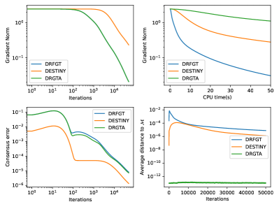
Figure 1: Convergence of DRFGT compared to DRGTA [24] and DESTINY [26].

We compare our performance with both a retraction-based algorithm DRFGT in [24] as well as the retraction-free DESTINY in [26]. We note that the learning rate for DESTINY is reduced to increase the stability of convergence. We present the results in Figure 1. We plot the system dynamics of gradient norm $\sum_{i\in[n]}\|\mathrm{grad}f_{i}(x_{i})\|_{\text{F}}$, consensus error $\sum_{i\in[n]}\|x_{i}-\bar{x}\|_{\text{F}}$, as well as the total distance to $\mathrm{St}(d,r)$, $\sum_{i\in[n]}\|x_{i}-x_{i}^{\prime}\|_{\text{F}}$, across different iterations. We can see that

• All three algorithms have $\mathcal{O}(\frac{1}{K})$ convergence rate when evaluated with log(x)-log(y) scale.

• For the same amount of iterations, DRFGT algorithm closely matches the performance of DRGTA, both of which are faster than DESTINY.

• DRFGT is much faster than DRGTA in computation time per iteration.

• While DRGTA stays feasible throughout the training process, DRFGT and DESTINY are able to gradually converge to the manifold.

VI Conclusion

We propose DRFGT to solve distributed optimization problems under orthogonality constraints, and provide a safety step-size to ensure DRFGT remains in the neighborhood of the Stiefel manifold. We show that the convergence rate for DRFGT is $\mathcal{O}(1/K)$, the first convergence result for the decentralized landing algorithm. Numerical results are provided as validation of our analysis. Future work of this paper include potential linear convergence for PCA-type tasks. DRFGT could also be extended to other manifold beyond the Stiefel manifold similar to [37].

Appendix

VI-A Proof for safety step size

Proposition VI.1 (Safe Step Size in Networks).

Let $\bar{x}\in\mathrm{St}(d,r)^{\frac{\epsilon}{2}}$ and $\|\mathbf{x}-\mathbf{1}\otimes\bar{x}\|_{\text{F}}^{2}\leq\frac{\epsilon}{2}$. Assuming that $\|\mathrm{grad}f(x)\|_{\text{F}}\leq G$, if the step size $\alpha$ satisfies

$$\alpha\leq\alpha_{safe} \triangleq\min\bigg{(}\frac{\lambda\epsilon(1-\frac{\epsilon}{4})(1-\sigma_{W})^{2}}{16L^{\prime}(G+\lambda\epsilon(1+\epsilon))},$$ (17)

$$\frac{(1-\sigma_{W})^{2}\epsilon}{4\sqrt{n}(G+\lambda\epsilon(1+\epsilon))},\frac{2\lambda\epsilon(2-\epsilon)}{16G^{2}+\lambda^{2}(1+\epsilon/2)\epsilon^{2}},$$

$$\frac{\sqrt{n}}{L^{\prime}},\sqrt{\frac{{\epsilon}}{8G^{2}}},\frac{1}{2\lambda}\bigg{)}$$

then the next iterate satisfy $\bar{x}^{+}\in\mathrm{St}(d,r)^{\frac{\epsilon}{2}}$ and $\|\mathbf{x}^{+}-\mathbf{1}\otimes\bar{x}^{+}\|_{\text{F}}^{2}\leq\frac{\epsilon}{2}$.

Proof.

We first show that $\|\mathbf{x}^{+}-\mathbf{1}\otimes\bar{x}^{+}\|_{\text{F}}^{2}$ stays in the region of $\frac{2\sqrt{n}\alpha(G+\lambda\epsilon(1+\epsilon))}{(1-\sigma_{W})^{2}}$.

We know that $\mathbf{x}_{k+1}=\mathbf{W}\mathbf{x}_{k}-\alpha\mathbf{y}_{k}$, then $\mathbf{x}_{k+1}-\mathbf{1}\otimes\bar{x}_{k+1}=\mathbf{W}(\mathbf{x}_{k}-\mathbf{1}\otimes\bar{x}_{k})-\alpha(\mathbf{y}_{k}-\mathbf{1}\otimes\bar{y}_{k})$, we get,

$$\|\mathbf{y}_{k+1}-\mathbf{1}\otimes\bar{y}_{k+1}\|_{\text{F}}$$

$$= \|\mathbf{W}(\mathbf{y}_{k}-\mathbf{1}\otimes\bar{y}_{k})-(\mathbf{u}_{k}-\mathbf{1}\otimes\bar{u}_{k}-\mathbf{u}_{k-1}+\mathbf{1}\otimes\bar{u}_{k-1})\|_{\text{F}}$$

$$\leq \|\mathbf{W}(\mathbf{y}_{k}-\mathbf{1}\otimes\bar{y}_{k})\|_{\text{F}}+\|(\mathbf{u}_{k}-\mathbf{u}_{k-1})\|_{\text{F}}$$

$$\leq \sigma_{W}\|\mathbf{y}_{k}-\mathbf{1}\otimes\bar{y}_{k}\|_{\text{F}}+\|\mathbf{u}_{k}\|_{\text{F}}+\|\mathbf{u}_{k-1}\|_{\text{F}}$$

$$\leq \sigma_{W}\|\mathbf{y}_{k}-\mathbf{1}\otimes\bar{y}_{k}\|_{\text{F}}+2\sqrt{n}(G+\lambda\epsilon(1+\epsilon))$$

The last inequality is from the assumption that all $x_{i,k}\in\mathrm{St}(d,r)^{\epsilon}$, and that $\|\mathrm{grad}f(x_{i,k})\|_{\text{F}}\leq G$

$\|\mathbf{y}_{k}-\mathbf{1}\otimes\bar{y}_{k}\|_{\text{F}}$ stays in the region of $\frac{2\sqrt{n}(G+\lambda\epsilon(1+\epsilon))}{1-\sigma_{W}}$.

$$\|\mathbf{x}_{k+1}-\mathbf{1}\otimes\bar{x}_{k+1}\|_{\text{F}}$$

$$= \|\mathbf{W}(\mathbf{x}_{k}-\mathbf{1}\otimes\bar{x}_{k})-\alpha(\mathbf{y}_{k}-\mathbf{1}\otimes\bar{y}_{k})\|_{\text{F}}$$

$$\leq \|\mathbf{W}(\mathbf{x}_{k}-\mathbf{1}\otimes\bar{x}_{k})\|_{\text{F}}+\alpha\|(\mathbf{y}_{k}-\mathbf{1}\otimes\bar{y}_{k})\|_{\text{F}}$$

$$\leq \sigma_{W}\|\mathbf{x}_{k}-\mathbf{1}\otimes\bar{x}_{k}\|_{\text{F}}+\alpha\|\mathbf{y}_{k}-\mathbf{1}\otimes\bar{y}_{k}\|_{\text{F}}$$

$$\leq \sigma_{W}\|\mathbf{x}_{k}-\mathbf{1}\otimes\bar{x}_{k}\|_{\text{F}}+\frac{2\alpha\sqrt{n}(G+\lambda\epsilon(1+\epsilon))}{1-\sigma_{W}}$$

$\|\mathbf{x}_{k}-\mathbf{1}\otimes\bar{x}_{k}\|_{\text{F}}$ will stay in the region $\frac{2\sqrt{n}\alpha(G+\lambda\epsilon(1+\epsilon))}{(1-\sigma_{W})^{2}}$,

We need

$$\alpha\leq\frac{(1-\sigma_{W})^{2}\epsilon}{4\sqrt{n}(G+\lambda\epsilon(1+\epsilon))}$$ (18)

Then $\|\mathbf{x}_{k+1}-\mathbf{1}\otimes\bar{x}_{k+1}\|_{\text{F}}\leq\frac{2\sqrt{n}\alpha(G+\lambda\epsilon(1+\epsilon))}{(1-\sigma_{W})^{2}}\leq\frac{\epsilon}{2}$.

Then we look to bound the distance of $\bar{x}_{k}$ from $\mathrm{St}(d,r)$. The proof closely follows Lemma 3 from [40]

From the definition of update on $\bar{x}_{k}$, we can write the actual update as the original landing field with an additional norm-bounded term. We denote the last term as $D_{k}$, and we can rewrite the update as

$$\bar{x}_{k+1}= \bar{x}_{k}-\alpha(\mathrm{grad}f(\bar{x}_{k})+\lambda\nabla p(\bar{x}_{k})+D_{k})$$

where

$$\|D_{k}\|_{\text{F}}= \|\bar{y}_{k}-\Lambda(\bar{x}_{k})\|_{\text{F}}$$

$$\leq \frac{L^{\prime}}{\sqrt{n}}\|\mathbf{x}_{k}-\mathbf{1}\otimes\bar{x}_{k}\|_{\text{F}}$$

$$\leq \frac{\epsilon L^{\prime}}{2\sqrt{n}}$$

We consider the worst case scenario, where we always have this term with the same direction as $-x(x^{\top}x-I_{r})$.

Now we consider two cases, at iteration $k$, we have (A) $\|\bar{x}_{k}^{\top}\bar{x}_{k}-I_{r}\|_{\text{F}}\leq\frac{\epsilon}{4}$ or (B) $\frac{\epsilon}{4}<\|\bar{x}_{k}^{\top}\bar{x}_{k}-I_{r}\|_{\text{F}}\leq\frac{\epsilon}{2}$.

VI-A1 Case A:

In this case, we want $\bar{x}_{k}-\alpha(\mathrm{grad}f(\bar{x}_{k})+\lambda\nabla p(\bar{x}_{k}))$ to not exit $\mathrm{St}(d,r)^{\frac{\epsilon}{4}}$ and $\alpha\|D_{k}\|_{\text{F}}\leq\frac{\epsilon}{4}$

For the first part, we can directly recall Lemma 4 in [40], and the safety step size here is

$$\alpha\leq\min(\frac{\lambda{\epsilon}(4-{\epsilon})}{16G^{2}+\lambda^{2}(1+\frac{\epsilon}{4}){\epsilon^{2}}},\sqrt{\frac{{\epsilon}}{8G^{2}}},\frac{1}{2\lambda})$$ (19)

For the second part, we need

$$\alpha\leq\frac{\sqrt{n}}{L^{\prime}}$$

VI-A2 Case B:

Case B: In this case, since the distance between $\bar{x}_{k}$ and $\mathrm{St}(d,r)$ is lower bounded, we divide the penalty into two terms, and show that $\bar{x}_{k}-\alpha(\mathrm{grad}f(\bar{x}_{k})+\frac{1}{2}\lambda\nabla p(\bar{x}_{k}))$ stays in $\mathrm{St}(d,r)^{\frac{\epsilon}{2}}$ and additionally, $\|\frac{1}{2}\lambda\nabla p(\bar{x}_{k})\|_{\text{F}}\geq\|D_{k}\|_{\text{F}}$ so that the iterated still stays inside $\mathrm{St}(d,r)^{\frac{\epsilon}{2}}$.

For the first part, we can apply Lemma 4 in [40] again, and get

$$\alpha\leq\min(\frac{2\lambda\epsilon(2-\epsilon)}{16G^{2}+\lambda^{2}(1+\epsilon/2)\epsilon^{2}},\sqrt{\frac{\epsilon}{4G^{2}}},\frac{1}{\lambda})$$ (20)

For the second part, since $\|\bar{x}_{k}^{\top}\bar{x}_{k}-I_{r}\|_{\text{F}}\geq\frac{\epsilon}{4}$, we have

$$\|\frac{1}{2}\lambda\nabla p(\bar{x}_{k})\|_{\text{F}}=\|\frac{1}{2}\lambda\bar{x}_{k}(\bar{x}_{k}^{\top}\bar{x}_{k}-I_{r})\|_{\text{F}}\geq\frac{\epsilon}{8}\lambda(1-\frac{\epsilon}{4})$$ (21)

We need

$$D_{k}\leq \frac{L^{\prime}}{\sqrt{n}}\|\mathbf{x}_{k}-\bar{x}_{k}\|_{\text{F}}$$

$$\leq \frac{2L^{\prime}\alpha(G+\lambda\epsilon(1+\epsilon))}{(1-\sigma_{W})^{2}}\leq\frac{\epsilon}{8}\lambda(1-\frac{\epsilon}{4})$$

$$\alpha\leq \frac{\lambda\epsilon(1-\frac{\epsilon}{4})(1-\sigma_{W})^{2}}{16L^{\prime}(G+\lambda\epsilon(1+\epsilon))}$$

Then in both cases, we have $\bar{x}_{k+1}\in\mathrm{St}(d,r)^{\frac{\epsilon}{2}}$, which completes the proof.

Combining all the requirements above on $\alpha$, we get

$$\alpha_{safe}= \min\bigg{(}\frac{\lambda\epsilon(1-\frac{\epsilon}{4})(1-\sigma_{W})^{2}}{16L^{\prime}(G+\lambda\epsilon(1+\epsilon))},\frac{\sqrt{n}}{L^{\prime}},\sqrt{\frac{\epsilon}{4G^{2}}},\frac{1}{\lambda},$$ (22)

$$\frac{2\lambda\epsilon(2-\epsilon)}{16G^{2}+\lambda^{2}(1+\epsilon/2)\epsilon^{2}},\frac{\lambda{\epsilon}(4-{\epsilon})}{16G^{2}+\lambda^{2}(1+\frac{\epsilon}{4}){\epsilon^{2}}},$$

$$\sqrt{\frac{{\epsilon}}{8G^{2}}},\frac{1}{2\lambda},\frac{(1-\sigma_{W})^{2}\epsilon}{4\sqrt{n}(G+\lambda\epsilon(1+\epsilon))}\bigg{)}$$

After simplification, the required safety step size is

$$\alpha\leq\alpha_{safe} \triangleq\min\bigg{(}\frac{\lambda\epsilon(1-\frac{\epsilon}{4})(1-\sigma_{W})^{2}}{16L^{\prime}(G+\lambda\epsilon(1+\epsilon))},$$

$$\frac{(1-\sigma_{W})^{2}\epsilon}{4\sqrt{n}(G+\lambda\epsilon(1+\epsilon))},\frac{2\lambda\epsilon(2-\epsilon)}{16G^{2}+\lambda^{2}(1+\epsilon/2)\epsilon^{2}},$$

$$\frac{\sqrt{n}}{L^{\prime}},\sqrt{\frac{{\epsilon}}{8G^{2}}},\frac{1}{2\lambda}\bigg{)}$$

∎

VI-B Proofs in Section IV-B

VI-B1 Proof of Lemma IV.2

Lemma VI.2.

Given Assumption III.5 with spectral norm $\sigma_{W}$, and step size $\alpha>0$. The Consensus error on $\mathbf{x}$ satisfies the following inequality,

$$\|\mathbf{x}_{k}-\bar{\mathbf{x}}_{k}\|_{\text{F}}^{2}\leq \frac{1+\sigma_{W}^{2}}{2}\|(\mathbf{x}_{k-1}-\mathbf{1}\otimes\bar{x}_{k-1})\|_{\text{F}}^{2}$$ (23)

$$+\frac{1+\sigma_{W}^{2}}{1-\sigma_{W}^{2}}\alpha^{2}\|\mathbf{y}_{k-1}-\bar{\mathbf{y}}_{k-1}\|_{\text{F}}$$

Proof.

$$\|\mathbf{x}_{k}-\bar{\mathbf{x}}_{k}\|_{\text{F}}^{2} =\|\mathbf{W}\mathbf{x}_{k-1}-\alpha\mathbf{y}_{k-1}-\bar{\mathbf{x}}_{k-1}+\alpha\bar{\mathbf{y}}_{k-1})\|_{\text{F}}^{2}$$

$$=\|\mathbf{W}(\mathbf{x}_{k-1}-\mathbf{1}\otimes\bar{x}_{k-1})-\alpha(\mathbf{y}_{k-1}-\mathbf{1}\otimes\bar{y}_{k-1})\|_{\text{F}}^{2}$$

From the definition of $\mathbf{W}$ and the spectral norm $\sigma_{W}$ from Assumption III.5,

$$\|\mathbf{x}_{k}-\bar{\mathbf{x}}_{k}\|_{\text{F}}^{2} =\|\mathbf{W}(\mathbf{x}_{k-1}-\bar{\mathbf{x}}_{k-1})-\alpha(\mathbf{y}_{k-1}-\bar{\mathbf{y}}_{k-1})\|_{\text{F}}^{2}$$

$$\leq(1+\kappa_{W})\|\mathbf{W}(\mathbf{x}_{k-1}-\bar{\mathbf{x}}_{k-1})\|_{\text{F}}^{2}$$

$$\quad+\frac{1+\kappa_{W}}{\kappa_{W}}\alpha^{2}\|\mathbf{y}_{k-1}-\bar{\mathbf{y}}_{k-1}\|_{\text{F}}$$

$$\leq(1+\kappa_{W})\sigma_{W}^{2}\|(\mathbf{x}_{k-1}-\bar{\mathbf{x}}_{k-1})\|_{\text{F}}^{2}$$

$$\quad+\frac{1+\kappa_{W}}{\kappa_{W}}\alpha^{2}\|\mathbf{y}_{k-1}-\bar{\mathbf{y}}_{k-1}\|_{\text{F}}$$

The inequality is obtained by expanding the Frobenius norm and applying Cauchy to the inner product term. We let $\kappa_{W}=\frac{1-\sigma_{W}^{2}}{2\sigma_{W}^{2}}$, and get:

$$\|\mathbf{x}_{k}-\bar{\mathbf{x}}_{k}\|_{\text{F}}^{2}\leq \frac{1+\sigma_{W}^{2}}{2}\|(\mathbf{x}_{k-1}-\bar{\mathbf{x}}_{k-1})\|_{\text{F}}^{2}$$

$$+\frac{1+\sigma_{W}^{2}}{1-\sigma_{W}^{2}}\alpha^{2}\|\mathbf{y}_{k-1}-\bar{\mathbf{y}}_{k-1}\|_{\text{F}}$$

Which completes the proof. ∎

VI-B2 Proof of Lemma IV.3

Lemma VI.3.

Let Assumption III.5 hold with spectral norm $\sigma_{W}$. The Consensus error on $\mathbf{y}$ satisfies the following inequality for $\alpha>0$,

$$\|\mathbf{y}_{k} -\bar{\mathbf{y}}_{k}\|_{\text{F}}^{2}\leq$$ (24)

$$\left(\frac{1+\sigma_{W}^{2}}{2}+4L^{\prime 2}\alpha^{2}\frac{1+\sigma_{W}^{2}}{1-\sigma_{W}^{2}}\right)\|\mathbf{y}_{k-1}-\bar{\mathbf{y}}_{k-1}\|_{\text{F}}^{2}$$

$$+2L^{\prime 2}\sigma_{W}^{2}\frac{1+\sigma_{W}^{2}}{1-\sigma_{W}^{2}}\|\mathbf{x}_{k-1}-\bar{\mathbf{x}}_{k-1}\|_{\text{F}}^{2}$$

$$+4L^{\prime 2}\alpha^{2}\frac{1+\sigma_{W}^{2}}{1-\sigma_{W}^{2}}\|\bar{\mathbf{y}}_{k-1}\|_{\text{F}}^{2}$$

Proof.

We first reiterate that $L<L_{\Lambda}\leq L^{\prime}$.

By definition of the update, we have

$$\|\mathbf{y}_{k}-\bar{\mathbf{y}}_{k}\|_{\text{F}}^{2}$$

$$= \|\mathbf{W}(\mathbf{y}_{k-1}-\bar{\mathbf{y}}_{k-1})+(\mathbf{u}_{k}-\bar{\mathbf{u}}_{k}-\mathbf{u}_{k-1}+\bar{\mathbf{u}}_{k-1})\|_{\text{F}}^{2}$$

Using the same technique as Lemma IV.2, we get

$$\leq \frac{1+\sigma_{W}^{2}}{2}\|\mathbf{y}_{k-1}-\bar{\mathbf{y}}_{k-1}\|_{\text{F}}^{2}$$

$$+\frac{1+\sigma_{W}^{2}}{1-\sigma_{W}^{2}}\|\mathbf{u}_{k}-\mathbf{1}\bar{\mathbf{u}}_{k}-\mathbf{u}_{k-1}+\bar{\mathbf{u}}_{k-1}\|_{\text{F}}^{2}$$

$$\leq \frac{1+\sigma_{W}^{2}}{2}\|\mathbf{y}_{k-1}-\bar{\mathbf{y}}_{k-1}\|_{\text{F}}^{2}+\frac{1+\sigma_{W}^{2}}{1-\sigma_{W}^{2}}\|\mathbf{u}_{k}-\mathbf{u}_{k-1}\|_{\text{F}}^{2}$$

$$\leq \frac{1+\sigma_{W}^{2}}{2}\|\mathbf{y}_{k-1}-\bar{\mathbf{y}}_{k-1}\|_{\text{F}}^{2}+\frac{1+\sigma_{W}^{2}}{1-\sigma_{W}^{2}}L^{\prime 2}\|\mathbf{x}_{k}-\mathbf{x}_{k-1}\|_{\text{F}}^{2}$$

$$= \frac{1+\sigma_{W}^{2}}{2}\|\mathbf{y}_{k-1}-\mathbf{1}\otimes\bar{y}_{k-1}\|_{\text{F}}^{2}$$

$$+\frac{1+\sigma_{W}^{2}}{1-\sigma_{W}^{2}}L^{\prime 2}\|(\mathbf{W}-\mathbf{I})\mathbf{x}_{k-1}+\alpha\mathbf{y}_{k-1}\|_{\text{F}}^{2}$$

$$\leq \frac{1+\sigma_{W}^{2}}{2}\|\mathbf{y}_{k-1}-\bar{\mathbf{y}}_{k-1}\|_{\text{F}}^{2}$$

$$+\frac{1+\sigma_{W}^{2}}{1-\sigma_{W}^{2}}L^{\prime 2}(2\|(\mathbf{W}-\mathbf{I})\mathbf{x}_{k-1}\|_{\text{F}}^{2}+2\|\alpha\mathbf{y}_{k-1}\|_{\text{F}}^{2})$$

$$\leq \frac{1+\sigma_{W}^{2}}{2}\|\mathbf{y}_{k-1}-\bar{\mathbf{y}}_{k-1}\|_{\text{F}}^{2}$$

$$+2L^{\prime 2}\sigma_{W}^{2}\frac{1+\sigma_{W}^{2}}{1-\sigma_{W}^{2}}\|\mathbf{x}_{k-1}-\bar{\mathbf{x}}_{k-1}\|_{\text{F}}^{2}$$

$$+2L^{\prime 2}\alpha^{2}\frac{1+\sigma_{W}^{2}}{1-\sigma_{W}^{2}}\|\mathbf{y}_{k-1}\|_{\text{F}}^{2}$$

Next for $\|\mathbf{y}_{k-1}\|_{\text{F}}^{2}$, we provide the following decomposition:

$$\|\mathbf{y}_{k-1}\|_{\text{F}}^{2}= \|\mathbf{y}_{k-1}-\bar{\mathbf{y}}_{k-1}+\bar{\mathbf{y}}_{k-1}\|_{\text{F}}^{2}$$

$$\leq 2\|\mathbf{y}_{k-1}-\bar{\mathbf{y}}_{k-1}\|_{\text{F}}^{2}+2\|\bar{\mathbf{y}}_{k-1}\|_{\text{F}}^{2}$$

plugging the inequality above into $\|\mathbf{y}_{k}-\bar{\mathbf{y}}_{k}\|_{\text{F}}^{2}$, we get

$$\|\mathbf{y}_{k}-\bar{\mathbf{y}}_{k}\|_{\text{F}}^{2}$$

$$\leq \left(\frac{1+\sigma_{W}^{2}}{2}+4L^{\prime 2}\alpha^{2}\frac{1+\sigma_{W}^{2}}{1-\sigma_{W}^{2}}\right)\|\mathbf{y}_{k-1}-\bar{\mathbf{y}}_{k-1}\|_{\text{F}}^{2}$$

$$+2L^{\prime 2}\sigma_{W}^{2}\frac{1+\sigma_{W}^{2}}{1-\sigma_{W}^{2}}\|\mathbf{x}_{k-1}-\bar{\mathbf{x}}_{k-1}\|_{\text{F}}^{2}$$

$$+4L^{\prime 2}\alpha^{2}\frac{1+\sigma_{W}^{2}}{1-\sigma_{W}^{2}}\|\bar{\mathbf{y}}_{k-1}\|_{\text{F}}^{2}$$

∎

VI-B3 Proof for Theorem IV.4

Theorem VI.4.

Suppose that the conditions for Lemma IV.2 and IV.3 are satisfied, we can write the system as a linear system with with state $\tilde{\xi}$, transition $\tilde{G}$ and input signal $\tilde{u}$,

$$\tilde{\xi}_{k}\leq\tilde{G}\tilde{\xi}_{k-1}+\tilde{u}_{k-1}.$$ (25)

with

$$\tilde{\xi}_{k} \triangleq\begin{bmatrix}\frac{\|\mathbf{y}_{k}-\bar{\mathbf{y}}_{k}\|_{\text{F}}^{2}}{L^{\prime}}\\ L^{\prime}\|\mathbf{x}_{k}-\bar{\mathbf{x}}_{k}\|_{\text{F}}^{2}\end{bmatrix},$$

$$\tilde{G} \triangleq\begin{bmatrix}\frac{1+\sigma_{W}^{2}}{2}+4L^{\prime 2}\alpha^{2}\frac{1+\sigma_{W}^{2}}{1-\sigma_{W}^{2}}&2\sigma_{W}^{2}\frac{1+\sigma_{W}^{2}}{1-\sigma_{W}^{2}}\\ \frac{1+\sigma_{W}^{2}}{1-\sigma_{W}^{2}}\alpha^{2}L^{\prime 2}&\frac{1+\sigma_{W}^{2}}{2}\end{bmatrix},$$

$$\tilde{u}_{k-1} \triangleq\begin{bmatrix}4L^{\prime}\alpha^{2}\frac{1+\sigma_{W}^{2}}{1-\sigma_{W}^{2}}\|\bar{\mathbf{y}}_{k}\|_{\text{F}}^{2}\\ 0\end{bmatrix}.$$

In addition, the linear system is stable, i.e. $\rho(\tilde{G})<1$ if

$$\alpha<\frac{(1-\sigma_{W}^{2})^{2}}{1+\sigma_{W}^{2}}\frac{1}{4L^{\prime}}.$$

Proof.

We need to ensure that $\rho(\tilde{G})<1$, which holds if and only if there exists solutions for the following inequalities.

$$\left(\frac{1+\sigma_{W}^{2}}{2}+4L^{\prime 2}\alpha^{2}\frac{1+\sigma_{W}^{2}}{1-\sigma_{W}^{2}}\right)s_{1}+2\sigma_{W}^{2}\frac{1+\sigma_{W}^{2}}{1-\sigma_{W}^{2}}s_{2} \leq s_{1}$$

$$\frac{1+\sigma_{W}^{2}}{1-\sigma_{W}^{2}}\alpha^{2}L^{\prime 2}s_{1}+\frac{1+\sigma_{W}^{2}}{2}s_{2} \leq s_{2}$$

solving this equation, we get

$$2\frac{(1+\sigma_{W}^{2})^{2}}{1-\sigma_{W}^{2}}\alpha^{2}L^{\prime 2}s_{1} \leq s_{2}$$

$$2\sigma_{W}^{2}\frac{1+\sigma_{W}^{2}}{1-\sigma_{W}^{2}}s_{2} \leq\left(\frac{1-\sigma_{W}^{2}}{2}-4L^{\prime 2}\alpha^{2}\frac{1+\sigma_{W}^{2}}{1-\sigma_{W}^{2}}\right)s_{1}$$

setting $s_{2}=8\frac{(1+\sigma_{W}^{2})^{2}}{1-\sigma_{W}^{2}}\alpha^{2}L^{\prime 2}s_{1}$, and with some inequality relaxation, we get the sufficient $\alpha$ such that

$$\alpha\leq\frac{(1-\sigma_{W}^{2})^{2}}{1+\sigma_{W}^{2}}\frac{1}{4L^{\prime}}$$

∎

VI-B4 Proof for Corollary IV.5

Corollary VI.5.

Given a stable step size $\alpha\leq\frac{(1-\sigma_{W}^{2})^{2}}{1+\sigma_{W}^{2}}\frac{1}{4L^{\prime}}$, we have the following upper bound:

$$\sum_{k}\|\mathbf{x}_{k}-\bar{\mathbf{x}}_{k}\|_{\text{F}}^{2} \leq\frac{1+\sigma_{W}^{2}}{(1-\sigma_{W}^{2})^{3}}8\alpha^{2}\|\mathbf{y}_{0}-\bar{\mathbf{y}}_{0}\|_{\text{F}}^{2}$$

$$+\frac{(1+\sigma_{W}^{2})^{2}}{(1-\sigma_{W}^{2})^{4}}32\alpha^{4}L^{\prime 2}\sum_{k}\|\bar{\mathbf{y}}_{k}\|_{\text{F}}^{2}$$

Proof.

We first calculate the determinant of $I-\tilde{G}$. Given that

$$I-\tilde{G} =\begin{bmatrix}1-\frac{1+\sigma_{W}^{2}}{2}-4L^{\prime 2}\alpha^{2}\frac{1+\sigma_{W}^{2}}{1-\sigma_{W}^{2}}&-2\sigma_{W}^{2}\frac{1+\sigma_{W}^{2}}{1-\sigma_{W}^{2}}\\ -\frac{1+\sigma_{W}^{2}}{1-\sigma_{W}^{2}}\alpha^{2}L^{\prime 2}&1-\frac{1+\sigma_{W}^{2}}{2}\end{bmatrix}$$

We can explicitly write

$$|I-\tilde{G}|= (\frac{1-\sigma_{W}^{2}}{2}-4L^{\prime 2}\alpha^{2}\frac{1+\sigma_{W}^{2}}{1-\sigma_{W}^{2}})\frac{1-\sigma_{W}^{2}}{2}$$

$$-\frac{1+\sigma_{W}^{2}}{1-\sigma_{W}^{2}}\alpha^{2}L^{\prime 2}2\sigma_{W}^{2}\frac{1+\sigma_{W}^{2}}{1-\sigma_{W}^{2}}$$

$$= (\frac{1-\sigma_{W}^{2}}{2})^{2}-2\alpha^{2}L^{\prime 2}((1+\sigma_{W}^{2})+\sigma_{W}^{2}\frac{(1+\sigma_{W}^{2})^{2}}{(1-\sigma_{W}^{2})^{2}})$$

Then in order to have $det(I-\tilde{G})\geq\frac{(1-\sigma_{W}^{2})^{2}}{8}$, we need

$$2\alpha^{2}L^{\prime 2}((1+\sigma_{W}^{2})+\sigma_{W}^{2}\frac{(1+\sigma_{W}^{2})^{2}}{(1-\sigma_{W}^{2})^{2}}) \leq\frac{(1-\sigma_{W}^{2})^{2}}{8}$$

$$\alpha^{2}L^{\prime 2}(\frac{1}{(1+\sigma_{W}^{2})}+\frac{\sigma_{W}^{2}}{(1-\sigma_{W}^{2})^{2}}) \leq\frac{1}{16L^{\prime 2}}$$

Which is satisfied when $\alpha\leq\frac{(1-\sigma_{W}^{2})^{2}}{1+\sigma_{W}^{2}}\frac{1}{4L^{\prime}}$.

Next, we note that

we note that

$$(I-\tilde{G})^{-1}=\frac{(I-\tilde{G})^{*}}{det(I-\tilde{G})}$$

$$\leq \frac{8}{(1-\sigma_{W}^{2})^{2}}\begin{bmatrix}\frac{1-\sigma_{W}^{2}}{2}-4L^{\prime 2}\alpha^{2}\frac{1+\sigma_{W}^{2}}{1-\sigma_{W}^{2}}&-2\sigma_{W}^{2}\frac{1+\sigma_{W}^{2}}{1-\sigma_{W}^{2}}\\ -\frac{1+\sigma_{W}^{2}}{1-\sigma_{W}^{2}}\alpha^{2}L^{\prime 2}&\frac{1-\sigma_{W}^{2}}{2}\end{bmatrix}^{*}$$

$$= \frac{8}{(1-\sigma_{W}^{2})^{2}}\begin{bmatrix}\frac{1-\sigma_{W}^{2}}{2}&2\sigma_{W}^{2}\frac{1+\sigma_{W}^{2}}{1-\sigma_{W}^{2}}\\ \frac{1+\sigma_{W}^{2}}{1-\sigma_{W}^{2}}\alpha^{2}L^{\prime 2}&\frac{1-\sigma_{W}^{2}}{2}-4L^{\prime 2}\alpha^{2}\frac{1+\sigma_{W}^{2}}{1-\sigma_{W}^{2}}\end{bmatrix}$$

$$= \begin{bmatrix}\frac{4}{1-\sigma_{W}^{2}}&16\sigma_{W}^{2}\frac{1+\sigma_{W}^{2}}{(1-\sigma_{W}^{2})^{3}}\\ \frac{1+\sigma_{W}^{2}}{(1-\sigma_{W}^{2})^{3}}8\alpha^{2}L^{\prime 2}&\frac{4}{1-\sigma_{W}^{2}}-32L^{\prime 2}\alpha^{2}\frac{1+\sigma_{W}^{2}}{(1-\sigma_{W}^{2})^{3}}\end{bmatrix}$$

The inequality is element-wise, with each entry non-negative.

Given that

$$\tilde{\xi}_{k}\leq\tilde{G}\tilde{\xi}_{k-1}+\tilde{u}_{k-1}.$$

We have

$$\tilde{\xi}_{k} \leq\tilde{G}^{k}\tilde{\xi}_{0}+\sum_{t=0}^{k}\tilde{G}^{t}\tilde{u}_{k-t-1}$$

$$\sum_{k=0}^{K}\tilde{\xi}_{k} \leq\sum_{k=0}^{K}\tilde{G}^{k}\tilde{\xi}_{0}+\sum_{k=0}^{K}\sum_{t=0}^{k}\tilde{G}^{t}\tilde{u}_{k-t-1}$$

$$\leq\sum_{k=0}^{\infty}\tilde{G}^{k}\tilde{\xi}_{0}+\sum_{k=0}^{K}\sum_{t=0}^{\infty}\tilde{G}^{t}\tilde{u}_{k-t-1}$$

$$=(I-\tilde{G})^{-1}\left(\tilde{\xi}_{0}+\sum_{k=0}^{K}\tilde{u}_{k}\right)$$

Given the inequality above, and the fact that $\|\mathbf{x}_{0}-\bar{\mathbf{x}}_{0}\|_{\text{F}}^{2}=0$, we know that

$$\sum_{k}L^{\prime} \|\mathbf{x}_{k}-\bar{\mathbf{x}}_{k}\|_{\text{F}}^{2}\leq\frac{1+\sigma_{W}^{2}}{(1-\sigma_{W}^{2})^{3}}8\alpha^{2}L^{\prime 2}\frac{1}{L^{\prime}}\|\mathbf{y}_{0}-\bar{\mathbf{y}}_{0}\|_{\text{F}}^{2}$$

$$+\frac{1+\sigma_{W}^{2}}{(1-\sigma_{W}^{2})^{3}}8\alpha^{2}L^{\prime 2}\sum_{k}4L^{\prime}\alpha^{2}\frac{1+\sigma_{W}^{2}}{1-\sigma_{W}^{2}}\|\bar{\mathbf{y}}_{k}\|_{\text{F}}^{2}$$

Therefore, we can write

$$\sum_{k}\|\mathbf{x}_{k}-\bar{\mathbf{x}}_{k}\|_{\text{F}}^{2} \leq\frac{1+\sigma_{W}^{2}}{(1-\sigma_{W}^{2})^{3}}8\alpha^{2}\|\mathbf{y}_{0}-\bar{\mathbf{y}}_{0}\|_{\text{F}}^{2}$$

$$+\frac{(1+\sigma_{W}^{2})^{2}}{(1-\sigma_{W}^{2})^{4}}32\alpha^{4}L^{\prime 2}\sum_{k}\|\bar{\mathbf{y}}_{k}\|_{\text{F}}^{2}$$

Which completes the proof. ∎

VI-C Proofs in Section IV-C

VI-C1 Proof for Lemma IV.6

Lemma VI.6.

Let Assumptions III.2 and III.5 hold and $\alpha$ satisfies the safety constraints in Proposition IV.1. The merit function (8) evaluated on $\bar{x}$ of Algorithm 1 satisfies the following inequality:

$$\mathcal{L}(\bar{x}_{k}) -\mathcal{L}(\bar{x}_{k-1})\leq-\frac{\alpha\rho}{2}\|\Lambda(\bar{x}_{k-1})\|_{\text{F}}^{2}$$ (26)

$$+\frac{\alpha C^{2}L^{2}}{2\rho n}\|\bar{\mathbf{x}}_{k-1}-\mathbf{x}_{k-1}\|_{\text{F}}^{2}+\frac{\alpha^{2}L^{\prime}}{2}\|\bar{y}_{k-1}\|_{\text{F}}^{2}$$

for any $\rho\geq 0$, $C=\frac{2L^{\prime}}{\lambda(1-\epsilon)}+1$.

In order to prove this lemma, we first need the following lemma:

Lemma VI.7.

For any $x\in\mathrm{St}(d,r)^{\epsilon}$, we have $\|\nabla\mathcal{L}(x)\|_{\text{F}}\leq C\|\Lambda(x)\|_{\text{F}}$, where $C=\frac{2L^{\prime}}{\lambda(1-\epsilon)}+1$

Proof.

We denote the projection of $x$ onto the Stiefel Manifold as $x^{\prime}=Proj_{\mathrm{St}}(x)$, from definition we know that $\nabla\mathcal{L}(x^{\prime})=\Lambda(x^{\prime})$

$$\|\nabla\mathcal{L}(x)\|_{\text{F}} =\|\nabla\mathcal{L}(x)-\nabla\mathcal{L}(x^{\prime})+\Lambda(x^{\prime})-\Lambda(x)+\Lambda(x)\|_{\text{F}}$$

$$\leq\|\nabla\mathcal{L}(x)-\nabla\mathcal{L}(x^{\prime})\|_{\text{F}}+\|\Lambda(x^{\prime})-\Lambda(x)\|_{\text{F}}+\|\Lambda(x)\|_{\text{F}}$$

$$\leq L^{\prime}\|x-x^{\prime}\|_{\text{F}}+L_{\Lambda}\|x-x^{\prime}\|_{\text{F}}+\|\Lambda(x)\|_{\text{F}}$$

since by definition, $\Lambda(x)=\mathrm{grad}f(x)+\lambda x(x^{\top}x-I_{r})$, we have

$$\|\Lambda(x)\|_{\text{F}}\geq\|\lambda x(x^{\top}x-I_{r})\|_{\text{F}}\geq\lambda(1-\epsilon)\|x^{\top}x-I_{r}\|_{\text{F}}$$

from Lemma 4.1 in paper, we have

$$\|x-x^{\prime}\|_{\text{F}}\leq\|x^{\top}x-I_{r}\|_{\text{F}}\leq(1+\epsilon)\|x-x^{\prime}\|_{\text{F}}.$$ (27)

Combining the properties above, we get

$$\|\nabla\mathcal{L}(x)\|_{\text{F}} \leq 2L^{\prime}\|x-x^{\prime}\|_{\text{F}}+\|\Lambda(x)\|_{\text{F}}$$

$$\leq 2L^{\prime}\|x^{\top}x-I_{r}\|_{\text{F}}+\|\Lambda(x)\|_{\text{F}}$$

$$\leq\left(\frac{2L^{\prime}}{\lambda(1-\epsilon)}+1\right)\|\Lambda(x)\|_{\text{F}}$$

∎

Then we can provide the proof of Lemma IV.6 below:

Proof.

$$\mathcal{L}(\bar{x}_{k})-\mathcal{L}(\bar{x}_{k-1})$$

$$\leq \langle\nabla\mathcal{L}(\bar{x}_{k-1}),\bar{x}_{k}-\bar{x}_{k-1}\rangle+\frac{L^{\prime}}{2}\|\bar{x}_{k}-\bar{x}_{k-1}\|_{\text{F}}^{2}$$

$$= -\alpha\langle\nabla\mathcal{L}(\bar{x}_{k-1}),\bar{y}_{k-1}\rangle+\frac{\alpha^{2}L^{\prime}}{2}\|\bar{y}_{k-1}\|_{\text{F}}^{2}$$

$$= -\alpha\langle\nabla\mathcal{L}(\bar{x}_{k-1}),\bar{y}_{k-1}-\Lambda(\bar{x}_{k-1})+\Lambda(\bar{x}_{k-1})\rangle$$

$$+\frac{\alpha^{2}L^{\prime}}{2}\|\bar{y}_{k-1}\|_{\text{F}}^{2}$$

$$= -\alpha\langle\nabla\mathcal{L}(\bar{x}_{k-1}),\Lambda(\bar{x}_{k-1})\rangle$$

$$-\alpha\langle\nabla\mathcal{L}(\bar{x}_{k-1}),\bar{y}_{k-1}-\Lambda(\bar{x}_{k-1})\rangle$$

$$+\frac{\alpha^{2}L^{\prime}}{2}\|\bar{y}_{k-1}\|_{\text{F}}^{2}$$

$$\leq -\alpha\rho\|\Lambda(\bar{x}_{k-1})\|_{\text{F}}^{2}-\alpha\langle\nabla\mathcal{L}(\bar{x}_{k-1}),\bar{y}_{k-1}-\Lambda(\bar{x}_{k-1})\rangle$$

$$+\frac{\alpha^{2}L^{\prime}}{2}\|\bar{y}_{k-1}\|_{\text{F}}^{2}$$

$$\leq -\alpha\rho\|\Lambda(\bar{x}_{k-1})\|_{\text{F}}^{2}+\frac{\alpha}{2\kappa}\|\nabla\mathcal{L}(\bar{x}_{k-1})\|_{\text{F}}^{2}$$

$$+\frac{\alpha\kappa}{2}\|\bar{y}_{k-1}-\Lambda(\bar{x}_{k-1})\|_{\text{F}}^{2}+\frac{\alpha^{2}L^{\prime}}{2}\|\bar{y}_{k-1}\|_{\text{F}}^{2}$$

$$\text{ With the help of Lemma \ref{lem:bound_C}, then setting }\kappa=\frac{C^{2}}{\rho}:$$

$$\leq -\alpha\rho\|\Lambda(\bar{x}_{k-1})\|_{\text{F}}^{2}+\frac{\alpha\rho}{2C^{2}}\|\nabla\mathcal{L}(\bar{x}_{k-1})\|_{\text{F}}^{2}$$

$$+\frac{\alpha C^{2}}{2\rho}\|\bar{y}_{k-1}-\Lambda(\bar{x}_{k-1})\|_{\text{F}}^{2}+\frac{\alpha^{2}L^{\prime}}{2}\|\bar{y}_{k-1}\|_{\text{F}}^{2}$$

$$\leq -\frac{\alpha\rho}{2}\|\Lambda(\bar{x}_{k-1})\|_{\text{F}}^{2}+\frac{\alpha C^{2}}{2\rho}\|\bar{y}_{k-1}-\Lambda(\bar{x}_{k-1})\|_{\text{F}}^{2}$$

$$+\frac{\alpha^{2}L^{\prime}}{2}\|\bar{y}_{k-1}\|_{\text{F}}^{2}$$

$$\leq -\frac{\alpha\rho}{2}\|\Lambda(\bar{x}_{k-1})\|_{\text{F}}^{2}+\frac{\alpha C^{2}L^{2}}{2\rho n}\|\bar{\mathbf{x}}_{k-1}-\mathbf{x}_{k-1}\|_{\text{F}}^{2}$$

$$+\frac{\alpha^{2}L^{\prime}}{2}\|\bar{y}_{k-1}\|_{\text{F}}^{2}$$

∎

VI-C2 Proof for Theorem IV.7

Theorem VI.8.

Suppose that the conditions for Theorem IV.4 and Lemma IV.6 are satisfied. If step-size $\alpha\leq\min\{\frac{\rho}{8L^{\prime}},\frac{1}{4L^{\prime}}\sqrt[3]{\frac{\rho(1-\sigma_{W}^{2})^{4}}{(1+\sigma_{W}^{2})^{2}C^{2}}}\}$, we get the following ergodic convergence:

$$\frac{\sum_{k}\|\Lambda(\bar{x}_{k-1})\|_{\text{F}}^{2}}{K}$$

$$\leq \frac{1}{K}\bigg{(}\frac{4}{\alpha\rho}(\mathcal{L}(\bar{x}_{0})-\mathcal{L}(\bar{x}_{K}))+\frac{32\alpha^{2}C^{2}L^{2}}{\rho^{2}n}\frac{1+\sigma_{W}^{2}}{(1-\sigma_{W}^{2})^{3}}\|\mathbf{y}_{0}-\bar{\mathbf{y}}_{0}\|_{\text{F}}^{2}\bigg{)}$$

$$\frac{\sum_{k}\|\mathbf{x}_{k}-\bar{\mathbf{x}}_{k}\|_{\text{F}}^{2}}{K}$$

$$\leq \frac{1}{K}\bigg{(}\frac{1+\sigma_{W}^{2}}{(1-\sigma_{W}^{2})^{3}}16\alpha^{2}(1+\frac{1}{\rho n})\|\mathbf{y}_{0}-\bar{\mathbf{y}}_{0}\|_{\text{F}}^{2}$$

$$+\frac{(1+\sigma_{W}^{2})^{2}}{(1-\sigma_{W}^{2})^{4}}\frac{512\alpha^{3}L^{\prime 2}}{\rho}(\mathcal{L}(\bar{x}_{0})-\mathcal{L}(\bar{x}_{K}))\bigg{)}.$$

Proof.

First, given $\bar{y}_{k-1}=\Lambda(\bar{x}_{k-1})+(\bar{y}_{k-1}-\Lambda(\bar{x}_{k-1}))$, it is easy to show

$$\|\bar{y}_{k-1}\|_{\text{F}}^{2}= \|\Lambda(\bar{x}_{k-1})+(\bar{y}_{k-1}-\Lambda(\bar{x}_{k-1}))\|_{\text{F}}^{2}$$

$$\leq 2\|\Lambda(\bar{x}_{k-1})\|_{\text{F}}^{2}+2\|\bar{y}_{k-1}-\Lambda(\bar{x}_{k-1})\|_{\text{F}}^{2}$$

Combining this with Lemma IV.6, we get

$$\mathcal{L}(\bar{x}_{k})-\mathcal{L}(\bar{x}_{k-1})$$

$$\leq -\frac{\alpha\rho}{2}\|\Lambda(\bar{x}_{k-1})\|_{\text{F}}^{2}+\frac{\alpha C^{2}L^{\prime 2}}{2\rho n}\|\bar{\mathbf{x}}_{k-1}-\mathbf{x}_{k-1}\|_{\text{F}}^{2}+\frac{\alpha^{2}L^{\prime}}{2}\|\bar{y}_{k-1}\|_{\text{F}}^{2}$$

$$\leq -\frac{\alpha\rho}{2}\|\Lambda(\bar{x}_{k-1})\|_{\text{F}}^{2}+\frac{\alpha C^{2}L^{\prime 2}}{2\rho n}\|\bar{\mathbf{x}}_{k-1}-\mathbf{x}_{k-1}\|_{\text{F}}^{2}$$

$$-\frac{\alpha^{2}L^{\prime}}{2}\|\bar{y}_{k-1}\|_{\text{F}}^{2}+2\alpha^{2}L^{\prime}\|\Lambda(\bar{x}_{k-1})\|_{\text{F}}^{2}+2\alpha^{2}L^{\prime}\|\bar{y}_{k-1}-\Lambda(\bar{x}_{k-1})\|_{\text{F}}^{2}$$

$$= -\left(\frac{\alpha\rho}{2}-2\alpha^{2}L^{\prime}\right)\|\Lambda(\bar{x}_{k-1})\|_{\text{F}}^{2}$$

$$+\left(\frac{\alpha C^{2}L^{\prime 2}}{2\rho n}+\frac{2\alpha^{2}L^{\prime 3}}{n}\right)\|\bar{\mathbf{x}}_{k-1}-\mathbf{x}_{k-1}\|_{\text{F}}^{2}-\frac{\alpha^{2}L^{\prime}}{2}\|\bar{y}_{k-1}\|_{\text{F}}^{2}$$

Since $\alpha\leq\frac{\rho}{8L^{\prime}}$, then in addition $\rho\leq\frac{1}{2}$,

$$\mathcal{L}(\bar{x}_{k})-\mathcal{L}(\bar{x}_{k-1})$$

$$\leq -\frac{\alpha\rho}{4}\|\Lambda(\bar{x}_{k-1})\|_{\text{F}}^{2}+\frac{\alpha L^{\prime 2}C^{2}}{\rho n}\|\bar{\mathbf{x}}_{k-1}-\mathbf{x}_{k-1}\|_{\text{F}}^{2}-\frac{\alpha^{2}L^{\prime}}{2}\|\bar{y}_{k-1}\|_{\text{F}}^{2}$$

Rearranging the terms, we get

$$\frac{\alpha\rho}{4}\|\Lambda(\bar{x}_{k-1})\|_{\text{F}}^{2}\leq \mathcal{L}(\bar{x}_{k-1})-\mathcal{L}(\bar{x}_{k})$$

$$+\frac{\alpha L^{\prime 2}C^{2}}{\rho n}\|\bar{\mathbf{x}}_{k-1}-\mathbf{x}_{k-1}\|_{\text{F}}^{2}-\frac{\alpha^{2}L^{\prime}}{2}\|\bar{y}_{k-1}\|_{\text{F}}^{2}$$

summing both sides,

$$\sum_{k}\frac{\alpha\rho}{4}\|\Lambda(\bar{x}_{k-1})\|_{\text{F}}^{2}$$

$$\leq \mathcal{L}(\bar{x}_{0})-\mathcal{L}(\bar{x}_{K})-\frac{\alpha^{2}L^{\prime}}{2}\sum_{k}\|\bar{y}_{k-1}\|_{\text{F}}^{2}$$

$$+\frac{\alpha L^{\prime 2}C^{2}}{\rho n}\sum_{k}\|\bar{\mathbf{x}}_{k-1}-\mathbf{x}_{k-1}\|_{\text{F}}^{2}$$

$$\leq \mathcal{L}(\bar{x}_{0})-\mathcal{L}(\bar{x}_{K})-\frac{\alpha^{2}L^{\prime}}{2}\sum_{k}\|\bar{y}_{k-1}\|_{\text{F}}^{2}$$

$$+\frac{\alpha L^{\prime 2}C^{2}}{\rho n}\frac{1+\sigma_{W}^{2}}{(1-\sigma_{W}^{2})^{3}}8\alpha^{2}\|\mathbf{y}_{0}-\bar{\mathbf{y}}_{0}\|_{\text{F}}^{2}$$

$$+\frac{\alpha L^{\prime 2}C^{2}}{\rho n}\frac{(1+\sigma_{W}^{2})^{2}}{(1-\sigma_{W}^{2})^{4}}32\alpha^{4}L^{\prime 2}\sum_{k}\|\bar{\mathbf{y}}_{k}\|_{\text{F}}^{2}$$

$$= \mathcal{L}(\bar{x}_{0})-\mathcal{L}(\bar{x}_{K})+\frac{\alpha C^{2}L^{2}}{\rho n}\frac{1+\sigma_{W}^{2}}{(1-\sigma_{W}^{2})^{3}}8\alpha^{2}\|\mathbf{y}_{0}-\bar{\mathbf{y}}_{0}\|_{\text{F}}^{2}$$

$$-\left(\frac{\alpha^{2}L^{\prime}}{2}-\frac{\alpha L^{\prime 2}C^{2}}{\rho}\frac{(1+\sigma_{W}^{2})^{2}}{(1-\sigma_{W}^{2})^{4}}32\alpha^{4}L^{\prime 2}\right)\sum_{k}\|\bar{y}_{k}\|_{\text{F}}^{2}$$

select $\alpha\leq\frac{1}{4L^{\prime}}\sqrt[3]{\frac{\rho(1-\sigma_{W}^{2})^{4}}{(1+\sigma_{W}^{2})^{2}C^{2}}}$ such that $\frac{\alpha^{2}L^{\prime}}{2}-\frac{\alpha L^{\prime 2}C^{2}}{\rho}\frac{(1+\sigma_{W}^{2})^{2}}{(1-\sigma_{W}^{2})^{4}}32\alpha^{4}L^{\prime 2}\geq 0$, we get the desired results

$$\frac{\sum_{k}\|\Lambda(\bar{x}_{k-1})\|_{\text{F}}^{2}}{K}$$

$$\leq \frac{1}{K}\bigg{(}\frac{4}{\alpha\rho}(\mathcal{L}(\bar{x}_{0})-\mathcal{L}(\bar{x}_{K}))$$

$$+\frac{32\alpha^{2}C^{2}L^{2}}{\rho^{2}n}\frac{1+\sigma_{W}^{2}}{(1-\sigma_{W}^{2})^{3}}\|\mathbf{y}_{0}-\bar{\mathbf{y}}_{0}\|_{\text{F}}^{2}\bigg{)}$$

In addition, the consensus can be bounded with

$$\sum_{k}\|\mathbf{x}_{k}-\bar{\mathbf{x}}_{k}\|_{\text{F}}^{2}$$

$$\leq \frac{1+\sigma_{W}^{2}}{(1-\sigma_{W}^{2})^{3}}8\alpha^{2}\|\mathbf{y}_{0}-\bar{\mathbf{y}}_{0}\|_{\text{F}}^{2}$$

$$+\frac{(1+\sigma_{W}^{2})^{2}}{(1-\sigma_{W}^{2})^{4}}32\alpha^{4}L^{\prime 2}\sum_{k}\|\bar{\mathbf{y}}_{k}\|_{\text{F}}^{2}$$

$$\leq \frac{1+\sigma_{W}^{2}}{(1-\sigma_{W}^{2})^{3}}8\alpha^{2}\|\mathbf{y}_{0}-\bar{\mathbf{y}}_{0}\|_{\text{F}}^{2}$$

$$+\frac{(1+\sigma_{W}^{2})^{2}}{(1-\sigma_{W}^{2})^{4}}32\alpha^{4}L^{\prime 2}\sum_{k}(2\|\Lambda(\bar{x}_{k-1})\|_{\text{F}}^{2}$$

$$\quad+2\|\bar{y}_{k-1}-\Lambda(\bar{x}_{k-1})\|_{\text{F}}^{2})$$

$$\leq \frac{1+\sigma_{W}^{2}}{(1-\sigma_{W}^{2})^{3}}8\alpha^{2}\|\mathbf{y}_{0}-\bar{\mathbf{y}}_{0}\|_{\text{F}}^{2}$$

$$+\frac{(1+\sigma_{W}^{2})^{2}}{(1-\sigma_{W}^{2})^{4}}64\alpha^{4}L^{\prime 2}\sum_{k}\|\Lambda(\bar{x}_{k-1})\|_{\text{F}}^{2}$$

$$+\frac{(1+\sigma_{W}^{2})^{2}}{(1-\sigma_{W}^{2})^{4}}\frac{64\alpha^{4}L^{\prime 4}}{n}\sum_{k}\|\mathbf{x}_{k-1}-\bar{\mathbf{x}}_{k-1}\|_{\text{F}}^{2}$$

Since we have $\alpha\leq\frac{1}{4L^{\prime}}\sqrt[3]{\frac{\rho(1-\sigma_{W}^{2})^{4}}{(1+\sigma_{W}^{2})^{2}C^{2}}},\rho\leq\frac{1}{2},C>1$, it is very easy to show that $\frac{(1+\sigma_{W}^{2})^{2}}{(1-\sigma_{W}^{2})^{4}}\frac{64\alpha^{4}L^{\prime 4}}{n}\leq\frac{1}{2}$, hence we can write

$$\sum_{k}\|\mathbf{x}_{k}-\bar{\mathbf{x}}_{k}\|_{\text{F}}^{2}\leq \frac{1+\sigma_{W}^{2}}{(1-\sigma_{W}^{2})^{3}}16\alpha^{2}\|\mathbf{y}_{0}-\bar{\mathbf{y}}_{0}\|_{\text{F}}^{2}$$

$$+\frac{(1+\sigma_{W}^{2})^{2}}{(1-\sigma_{W}^{2})^{4}}128\alpha^{4}L^{\prime 2}\sum_{k}\|\Lambda(\bar{x}_{k-1})\|_{\text{F}}^{2}$$

$$\frac{\sum_{k}\|\mathbf{x}_{k}-\bar{\mathbf{x}}_{k}\|_{\text{F}}^{2}}{K}\leq \frac{1}{K}\bigg{(}\frac{1+\sigma_{W}^{2}}{(1-\sigma_{W}^{2})^{3}}16\alpha^{2}\|\mathbf{y}_{0}-\bar{\mathbf{y}}_{0}\|_{\text{F}}^{2}$$

$$+\frac{(1+\sigma_{W}^{2})^{2}}{(1-\sigma_{W}^{2})^{4}}\frac{512\alpha^{3}L^{\prime 2}}{\rho}(\mathcal{L}(\bar{x}_{0})-\mathcal{L}(\bar{x}_{K}))$$

$$+\frac{(1+\sigma_{W}^{2})^{3}}{(1-\sigma_{W}^{2})^{7}}\frac{4096\alpha^{6}L^{\prime 4}C^{2}}{\rho^{2}n}\|\mathbf{y}_{0}-\bar{\mathbf{y}}_{0}\|_{\text{F}}^{2})\bigg{)}$$

$$\leq \frac{1}{K}\bigg{(}\frac{1+\sigma_{W}^{2}}{(1-\sigma_{W}^{2})^{3}}16\alpha^{2}(1+\frac{1}{\rho n})\|\mathbf{y}_{0}-\bar{\mathbf{y}}_{0}\|_{\text{F}}^{2}$$

$$+\frac{(1+\sigma_{W}^{2})^{2}}{(1-\sigma_{W}^{2})^{4}}\frac{512\alpha^{3}L^{\prime 2}}{\rho}(\mathcal{L}(\bar{x}_{0})-\mathcal{L}(\bar{x}_{K}))\bigg{)}$$

∎

References

• [1] P. Ablin and G. Peyré, “Fast and accurate optimization on the orthogonal manifold without retraction,” in International Conference on Artificial Intelligence and Statistics.   PMLR, 2022, pp. 5636–5657.
• [2] H. Hotelling, “Analysis of a complex of statistical variables into principal components.” Journal of educational psychology, vol. 24, no. 6, p. 417, 1933.
• [3] ——, “Canonical correlation analysis (cca),” Journal of Educational Psychology, vol. 10, pp. 12 913–2, 1935.
• [4] D. Kempe and F. McSherry, “A decentralized algorithm for spectral analysis,” Journal of Computer and System Sciences, vol. 74, no. 1, pp. 70–83, 2008.
• [5] N. Kishore Kumar and J. Schneider, “Literature survey on low rank approximation of matrices,” Linear and Multilinear Algebra, vol. 65, no. 11, pp. 2212–2244, 2017.
• [6] H. Raja and W. U. Bajwa, “Cloud k-svd: A collaborative dictionary learning algorithm for big, distributed data,” IEEE Transactions on Signal Processing, vol. 64, no. 1, pp. 173–188, 2015.
• [7] M. Arjovsky, A. Shah, and Y. Bengio, “Unitary evolution recurrent neural networks,” in International Conference on Machine Learning.   PMLR, 2016, pp. 1120–1128.
• [8] E. Vorontsov, C. Trabelsi, S. Kadoury, and C. Pal, “On orthogonality and learning recurrent networks with long term dependencies,” in International Conference on Machine Learning.   PMLR, 2017, pp. 3570–3578.
• [9] A. Trockman and J. Z. Kolter, “Orthogonalizing convolutional layers with the cayley transform,” arXiv preprint arXiv:2104.07167, 2021.
• [10] Q. Zhang, M. Chen, A. Bukharin, P. He, Y. Cheng, W. Chen, and T. Zhao, “Adaptive budget allocation for parameter-efficient fine-tuning,” arXiv preprint arXiv:2303.10512, 2023.
• [11] P.-A. Absil and J. Malick, “Projection-like retractions on matrix manifolds,” SIAM Journal on Optimization, vol. 22, no. 1, pp. 135–158, 2012.
• [12] N. Boumal, P.-A. Absil, and C. Cartis, “Global rates of convergence for nonconvex optimization on manifolds,” IMA Journal of Numerical Analysis, vol. 39, no. 1, pp. 1–33, 2019.
• [13] H. Zhang and S. Sra, “First-order methods for geodesically convex optimization,” in Conference on Learning Theory.   PMLR, 2016, pp. 1617–1638.
• [14] J. Tsitsiklis, D. Bertsekas, and M. Athans, “Distributed asynchronous deterministic and stochastic gradient optimization algorithms,” IEEE transactions on automatic control, vol. 31, no. 9, pp. 803–812, 1986.
• [15] A. Nedic and A. Ozdaglar, “Distributed subgradient methods for multi-agent optimization,” IEEE Transactions on Automatic Control, vol. 54, no. 1, pp. 48–61, 2009.
• [16] S. Chen, A. Garcia, and S. Shahrampour, “On distributed nonconvex optimization: Projected subgradient method for weakly convex problems in networks,” IEEE Transactions on Automatic Control, vol. 67, no. 2, pp. 662–675, 2021.
• [17] G. Qu and N. Li, “Harnessing smoothness to accelerate distributed optimization,” IEEE Transactions on Control of Network Systems, vol. 5, no. 3, pp. 1245–1260, 2017.
• [18] W. Shi, Q. Ling, G. Wu, and W. Yin, “Extra: An exact first-order algorithm for decentralized consensus optimization,” SIAM Journal on Optimization, vol. 25, no. 2, pp. 944–966, 2015.
• [19] P. Di Lorenzo and G. Scutari, “Next: In-network nonconvex optimization,” IEEE Transactions on Signal and Information Processing over Networks, vol. 2, no. 2, pp. 120–136, 2016.
• [20] Y. Sun, M. Fazlyab, and S. Shahrampour, “On centralized and distributed mirror descent: Convergence analysis using quadratic constraints,” IEEE Transactions on Automatic Control, 2022.
• [21] A. Sarlette and R. Sepulchre, “Consensus optimization on manifolds,” SIAM journal on Control and Optimization, vol. 48, no. 1, pp. 56–76, 2009.
• [22] S. Chen, A. Garcia, M. Hong, and S. Shahrampour, “On the local linear rate of consensus on the stiefel manifold,” IEEE Transactions on Automatic Control, pp. 1–16, 2023.
• [23] H. Ye and T. Zhang, “Deepca: Decentralized exact pca with linear convergence rate,” The Journal of Machine Learning Research, vol. 22, no. 1, pp. 10 777–10 803, 2021.
• [24] S. Chen, A. Garcia, M. Hong, and S. Shahrampour, “Decentralized riemannian gradient descent on the stiefel manifold,” in International Conference on Machine Learning.   PMLR, 2021, pp. 1594–1605.
• [25] K. Deng and J. Hu, “Decentralized projected riemannian gradient method for smooth optimization on compact submanifolds,” arXiv preprint arXiv:2304.08241, 2023.
• [26] L. Wang and X. Liu, “Decentralized optimization over the stiefel manifold by an approximate augmented lagrangian function,” IEEE Transactions on Signal Processing, vol. 70, pp. 3029–3041, 2022.
• [27] L. Wang, L. Bao, and X. Liu, “A decentralized proximal gradient tracking algorithm for composite optimization on riemannian manifolds,” arXiv preprint arXiv:2401.11573, 2024.
• [28] J. Chen, H. Ye, M. Wang, T. Huang, G. Dai, I. Tsang, and Y. Liu, “Decentralized riemannian conjugate gradient method on the stiefel manifold,” in The Twelfth International Conference on Learning Representations, 2023.
• [29] P.-A. Absil, R. Mahony, and R. Sepulchre, Optimization algorithms on matrix manifolds.   Princeton University Press, 2008.
• [30] C. Qi, K. A. Gallivan, and P.-A. Absil, “Riemannian bfgs algorithm with applications,” in Recent Advances in Optimization and its Applications in Engineering: The 14th Belgian-French-German Conference on Optimization.   Springer, 2010, pp. 183–192.
• [31] Y. Liu, F. Shang, J. Cheng, H. Cheng, and L. Jiao, “Accelerated first-order methods for geodesically convex optimization on riemannian manifolds,” Advances in Neural Information Processing Systems, vol. 30, 2017.
• [32] N. Bansal, X. Chen, and Z. Wang, “Can we gain more from orthogonality regularizations in training deep networks?” Advances in Neural Information Processing Systems, vol. 31, 2018.
• [33] R. Balestriero and R. G. Baraniuk, “Mad max: Affine spline insights into deep learning,” Proceedings of the IEEE, vol. 109, no. 5, pp. 704–727, 2020.
• [34] B. Gao, X. Liu, and Y.-x. Yuan, “Parallelizable algorithms for optimization problems with orthogonality constraints,” SIAM Journal on Scientific Computing, vol. 41, no. 3, pp. A1949–A1983, 2019.
• [35] N. Xiao, X. Liu, and Y.-x. Yuan, “A penalty-free infeasible approach for a class of nonsmooth optimization problems over the stiefel manifold,” arXiv preprint arXiv:2103.03514, 2021.
• [36] S. Schechtman, D. Tiapkin, M. Muehlebach, and E. Moulines, “Orthogonal directions constrained gradient method: from non-linear equality constraints to stiefel manifold,” arXiv preprint arXiv:2303.09261, 2023.
• [37] N. Xiao, X. Liu, and K.-C. Toh, “Dissolving constraints for riemannian optimization,” Mathematics of Operations Research, vol. 49, no. 1, pp. 366–397, 2024.
• [38] A. Edelman, T. A. Arias, and S. T. Smith, “The geometry of algorithms with orthogonality constraints,” SIAM journal on Matrix Analysis and Applications, vol. 20, no. 2, pp. 303–353, 1998.
• [39] Z. Wen and W. Yin, “A feasible method for optimization with orthogonality constraints,” Mathematical Programming, vol. 142, no. 1-2, pp. 397–434, 2013.
• [40] P. Ablin, S. Vary, B. Gao, and P.-A. Absil, “Infeasible deterministic, stochastic, and variance-reduction algorithms for optimization under orthogonality constraints,” arXiv preprint arXiv:2303.16510, 2023.
• [41] J. C. Gower and G. B. Dijksterhuis, Procrustes problems.   OUP Oxford, 2004, vol. 30.