Probing Massive Fields with Multi-Band Gravitational-Wave Observations

Abstract

We investigate the prospect of probing massive fields and testing gravitational theories with multi-band observations of gravitational waves emitted from coalescing compact binaries. Focusing on the dipole radiation induced by a massive field, we show that multi-band observations can probe the field with mass ranging from $10^{-16}{\rm eV}$ to $10^{-15}{\rm eV}$, a parameter space that cannot be probed by the milli-Hertz band observations alone. Multi-band observations can also improve the constraints obtained with the LIGO-Virgo-KAGRA binaries by at most 3 orders of magnitude in the mass range. Moreover, we show that multi-band observations can discriminate the spin of the field, which cannot be identified with single band observations.

I Introduction

The existence of particles beyond standard model is not only predicted by fundamental theories, but also implied by observations of dark matter and dark energy. These new particles may weakly couple to the stand model particles, but could still get excited in extreme gravitational environments. It is known that, fields of the new particles, such as light axions, generalized Proca and extra degrees of freedom in gravity beyond general relativity (GR), can be significantly excited by neutron stars and black holes due to instability [1, 2, 3, 4, 5], nonlinearity [6, 7] and other mechanisms [8, 9, 10], providing promising ways of searching for physics beyond the standard model. For example, superradiantly excited axions around supermassive black holes can induce additional polarization of light, and hence are constrained with Event Horizon Telescope [11, 12].

In recent years, gravitational waves (GWs) emitted by coalescing compact binaries have became a valuable probe to the physics in extreme gravitational environments. Deviations from GR and the standard model are searched and constrained by analyzing GW signals observed by the LIGO-Virgo-KAGRA (LVK) collaboration [13, 14, 15, 16, 17]. Also see, e.g., Refs. [18, 19, 20, 21, 22] and the references therein. With such a success in territorial detections, space-borne GW interferometers, such as LISA, Tianqin, and Taiji, are planned to launch by the mid-2030s. These space-borne detectors target GWs of milli-Hertz (mHz) frequencies, which are complementary to the LVK band, and hence will probe fundamental physics from different approaches.

Interestingly, about $10$-$1000$ stellar mass black hole binaries are expected to be observed in both the mHz band and the LVK band [23], opening the prospect for multi-band GW astronomy. These binaries first inspiral in the mHz band for several years, and then re-appear in the LVK band typically a few weeks before they merge. Due to the long persistence of the signal in the mHz band, space-borne detectors can measure the masses and sky location of the binaries with great accuracy, while LVK and future territorial detectors can measure the GW amplitude better due to the high signal to noise ratio (SNR). Therefore, multi-band detection shall significantly improve parameter estimation in GW sources, and will be ideal for probing fundamental physics [24], such as constraining post-Newtonian (PN) and post-Einsteinian (PE) deviations [25, 26, 27, 28, 29], searching for dipole GW radiation [30, 31, 32, 33], measuring GW dispersion relation [34, 35], performing consistency tests [24, 36, 27] and bounding alternative gravity theories [36].

In this work, we emphasize the prospect of probing new massive bosonic fields with multi-band GW observations. For massless (or ultralight) bosonic fields, their effects on orbital dynamics can be captured by parameterized PN and PE formalisms, and have been constrained with the Hulse-Taylor pulsar [37, 38, 39, 40], LVK binaries [17] and pulsar timing arrays[41]. Detectability of such fields with future GW detectors and multi-band observations is also forecasted in the literature [42, 43, 44, 45]. Effects of a massive field, however, do not generally fit with the parameterized PN or PE formalism, and should be treated separately. In particular, for fields with masses heavier than $10^{-16}{\rm eV}$, their effects are suppressed for inspirals in the mHz band [46, 47, 48, 44, 49]. Yet, they can be constrained with LVK binaries to certain accuracy, if their mass is below $10^{-11}{\rm eV}$ [50]. In this work, we shall demonstrate that constraints on massive fields can be significantly improved by 3 orders of magnitude with multi-band observations, especially for the fields with mass ranging in $10^{-16}{\rm eV}-10^{-15}{\rm eV}$, which cannot be well probed by space-born GW detectors. Moreover, we find that multi-band GW observations can distinguish the spin of the field, if its mass is within $10^{-16}-10^{-15}{\rm eV}$, which is hardly done with single band observations. We work in the units of $G=\hbar=c=1$.

II Inspirals with massive fields

Though the excitation mechanism depends on the theories, the new field, once excited by the compact object, typically affects binary inspirals by mediating additional force and emitting additional radiation. While the force could modify the inspiral waveform at $0$ PN order, the additional radiation usually manifests at $-1$ PN order, and hence is the main signature that we are after.

To be concrete, we start from a massive spin-0 field with following action,

$$S=\int\mathrm{d}^{4}x\sqrt{-g}\left(\frac{1}{2}\nabla_{\mu}\varphi\nabla^{\mu}\varphi-\frac{1}{2}\mu^{2}\varphi^{2}+\mathcal{L}_{\rm int}\right)$$ (1)

where $\varphi$ is the spin-0 field of mass $\mu$, and $\mathcal{L}_{\rm int}$ denotes the interaction between the field and the matter fields. During early inspiral, the two compact objects in a binary can be treated as two non-relativistic point-like particles. In this case, the leading order interaction term is

$$\mathcal{L}_{\rm int}\simeq\sum_{i=1,2}\sqrt{2}\,Q_{i}\delta\left({\bf x}-{\bf x}_{i}(t)\right)\varphi(t,{\bf x})\,,$$ (2)

where $Q_{i}$ and ${\bf x}_{i}(t)$ represent the charge and position of the $i$-th object respectively. We shall also consider a massive spin-1 field, the action of which is

$$S=\int\mathrm{d}^{4}x\sqrt{-g}\left(-\frac{1}{4}F_{\mu\nu}F^{\mu\nu}-\frac{1}{2}\mu^{2}A_{\mu}A^{\mu}+\mathcal{L}_{\rm int}\right)\,,$$ (3)

where $F_{\mu\nu}=\nabla_{\mu}A_{\nu}-\nabla_{\nu}A_{\mu}$. The spin-1 field couples to matter fields through their current $J^{\mu}$, i.e., $\mathcal{L}_{\rm int}\propto A_{\mu}J^{\mu}$. Again, treating the binary as two non-relativistic point-like particles, the coupling becomes

$$\mathcal{L}_{\rm int}\simeq\sum_{i=1,2}Q_{i}\delta\left({\bf x}-{\bf x}_{i}(t)\right)A^{0}(t,{\bf x})\,.$$ (4)

In principle, one can consider massive spin-2 field which presents, for example, in bi-gravity. However, defining energy flux is subtle in theories with two dynamical metrics [51]. It is also possible that the graviton itself has a non-zero but tiny mass, and GR should be replaced by a massive gravity theory. In this case, nonlinearity is expected to be important within the so-call Vainshtein radius, a scale that is typically much larger than the size of stellar mass binary. As a results, deviations from GR, including radiations of extra degrees of freedom in massive gravity, are expected to be suppressed for stellar mass binaries. For these reasons, we shall focus on and demonstrate the multi-band detection strategy with only spin-0 and spin-1 fields.

Given the actions (1) and (3), one can calculate the energy flux carrying by the radiations of the massive fields. For circular orbits, the energy flux of dipole radiation is given by

$$P_{\rm MF}=\frac{2}{3}\Delta q^{2}\left(\frac{m_{1}m_{2}}{m_{1}+m_{2}}\right)^{2}R^{2}\Omega^{4}\,g\left(\Omega,\mu\right)$$ (5)

with

$$g\left(\Omega,\mu\right)=\left\{\begin{aligned} &\left[1-\left(\tfrac{\mu}{\Omega}\right)^{2}\right]^{3/2}\,&\text{spin-0}\\ &\sqrt{1-\left(\tfrac{\mu}{\Omega}\right)^{2}}\left[1+\frac{1}{2}\left(\tfrac{\mu}{\Omega}\right)^{2}\right]&\text{spin-1}\end{aligned}\right.\,,$$ (6)

where $R$ is the orbital separation, $\Omega$ is the orbital frequency and $\Delta q\equiv\left(Q_{1}/m_{1}\right)-\left(Q_{2}/m_{2}\right)$ with $m_{1,2}$ being the mass of compact objects. See, e.g., Ref. [52] for details. The models we considered here is generic, and hence the energy flux calculated by Eq. (5) applies to many theories, see Refs. [53, 54, 55, 56, 57, 44, 58, 59, 60] for example.

To incorporate the effects of the dipole radiation from the massive fields into inspiral waveform, we calculate the waveform in frequency domain by extending the TaylorF2 template. Specifically, the waveform template is given in frequency domain,

$$h(f)\simeq H(f)\exp\left[i\Psi(f)\right]\,,$$ (7)

where $\Psi(f)=2\pi ft-\phi-\tfrac{\pi}{4}$ is the GW phase, and is calculated under the stationary phase approximation,

$$t(f) = t_{c}-\int_{f_{c}}^{f}\frac{1}{P}\left(\frac{dE}{df^{\prime}}\right)\mathrm{d}f^{\prime}\,,$$ (8)

$$\phi(f) = \phi_{c}-\int_{f_{c}}^{f}\frac{2\pi f^{\prime}}{P}\left(\frac{dE}{df^{\prime}}\right)\mathrm{d}f^{\prime}\,.$$ (9)

Here $E$ and $P$ are binding energy and total radiation power of the binary system, while $t_{c}$ and $\phi_{c}$ are the time and phase at merger. In the presence of a massive field, the total radiation power can be written as $P=P_{\rm GR}+P_{\rm MF}$. Namely, it includes energy fluxes of both GWs in GR and radiation of the massive field. Assuming $|\Delta q|\ll 1$, the massive field induces an extra phase $\Psi_{\rm MF}$ in the waveform,

$$\Psi(f)\approx\Psi_{\rm GR}(f)+\Psi_{\rm MF}(f),$$ (10)

where $\Psi_{\rm GR}$ is the GW phase predicted by GR, and the explicit expression of $\Psi_{\rm MF}$ is given in App. A.

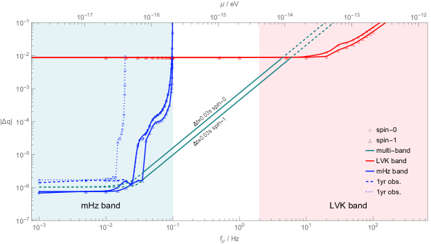
Figure 1: Detectability on spin-0 and spin-1 fields of different mass. The markers show the expectation errors on $\Delta q$ obtained by calculating the Fisher information matrix (cf. Eq. (19)), assuming a GW150914-like event observed in the mHz and the LVK bands. Here circles and triangles show the errors for spin-0 and spin-1 fields respectively, while blue and red denote the mHz and the LVK bands. For observations in the mHz bands, markers jointed by the solid, dashed and dotted lines show the situation of a $4$-year observation starting at $4$ years before merger, a $1$-year observation starting at $1$ year before merger and a $1$-year observation starting at $4$ years before merger respectively. The green lines show the merger time deviation from GR, when there is a spin-0 or a spin-1 massive field.

III Single-band observations

Given the inspiral waveform, we first investigate detectability of the massive fields with single band observations. It is convenient to introduce

$$f_{\mu}\equiv\frac{\mu}{\pi}=0.48\times\left(\frac{\mu}{10^{-15}{\rm eV}}\right){\rm Hz}\,.$$ (11)

In the LVK band, we expect to observe the binary coalescence up to merger, and the phase shift induced by dipole radiation of the massive field can be estimated as

$$\Psi_{\rm MF}(f)\sim\frac{5}{2688}\Delta q^{2}\nu^{-1}\left(\pi Mf\right)^{-7/3}\,,$$ (12)

with $M=m_{1}+m_{2}$ and $\nu=m_{1}m_{2}/M^{2}$. Here $f$ should be $f_{\mu}$ or $f_{i}$, whichever is larger, with $f_{i}\sim 2{\rm Hz}$ being the GW frequency when the inspiral signal enters the LVK band. Assuming the dipole radiation can be detected if $\Psi_{\rm MF}\sim{\cal O}(1)$, we expect that detectors in the LVK band are sensitive to $\Delta q\gtrsim 0.008$ for fields with $f_{\mu}<f_{i}$, and the sensitivity gets worse as $f_{\mu}$ increases. We shall also estimate the detectability with observations in the mHz band. Different from the LVK band, we may not observe a clear chirping in GW frequncy during the observation time, if the binary is in its very early inspiral stage when the detector turns on. In particular, the time to merger given by GR is

$$\tau_{\rm GR} \simeq \frac{5}{256}M\nu^{-1}\left(\pi Mf_{i}\right)^{-8/3}$$

$$\approx 1.03\,{\rm yrs}\left(\frac{\nu}{0.25}\right)^{-1}\left(\frac{M}{60M_{\odot}}\right)^{-5/3}\left(\frac{f_{i}}{\rm 0.03Hz}\right)^{-8/3}.$$

Therefore, if the binary is emitting GWs with $f_{i}\gtrsim 0.03{\rm Hz}$ when detector turns on, the signal will leave the mHz band during the observation period, which is typically assumed to be $1$ year or $4$ years. The phase shift induced by the dipole radiation during the observation time can still be estimated with Eq. (12), and we expect the minimally detectable $\Delta q$ is $\sim 6\times 10^{-5}$ for $f_{\mu}<f_{i}$. On the other hands, for $f_{i}\ll 0.03{\rm Hz}$, we do not expect to see $f$ changes significantly during the operating time, and the detector can only probe the dipole radiation of fields with $f_{\mu}\lesssim f_{i}<0.03{\rm Hz}$. In this case, the additional phase shift is given by

$$\Psi_{\rm MF}\sim\frac{2}{21}\Delta q^{2}(\pi Mf_{i})^{1/3}M^{-1}T_{\rm obs}\,,$$ (14)

where $T_{\rm obs}$ is operating time. The minimally detectable $|\Delta q|$ is $\sim 3\times 10^{-5}$ assuming a $4$-year observation. Comparing to the LVK band, observations in the mHz band generally have better accuracy for fields with $f_{\mu}\lesssim 0.01{\rm Hz}$. However, the accuracy gets worse quickly as $f_{\mu}$ increases. In fact, observations in the mHz band almost cannot probe fields with $f_{\mu}>0.1{\rm Hz}$, because the massive field almost plays no role during the entire observation.

A rigorous forecast on detectability can be made using Fisher information matrix. Having in mind an interferometric detector and working in frequency domain, the measured date $d$ can be expressed as a linear combination of the signal $s$ and the detector noise $n$,

$$d(f)=s(f,{\bm{\theta}})+n(f).$$ (15)

The signal is the detector response to GWs that are characterized by a set of parameters ${\bm{\theta}}$. Assuming the noise to be stationary and Gaussian with a single-sided spectral density $S_{n}\left(f\right)$, the likelihood is

$${\cal L}\left(d|{\bm{\theta}}\right)\propto\exp\left[-\frac{1}{2}\langle d-s({\bm{\theta}})|d-s({\bm{\theta}})\rangle\right]\,,$$ (16)

where the inner product is defined by

$$\langle a|b\rangle=2\int_{-\infty}^{+\infty}\frac{a(f)b^{*}(f)+a^{*}(f)b(f)}{S_{n}(f)}\,\mathrm{d}f\,.$$ (17)

For signals with large SNR, the detectability of the signal characterized by ${\bm{\theta}}_{0}$ can be forecasted with Fisher information matrix,

$$\Gamma_{ij}=\left.\left\langle\frac{\partial s}{\partial\theta_{i}}\right|\left.\frac{\partial s}{\partial\theta_{j}}\right\rangle\right|_{{\bm{\theta}}={\bm{\theta}}_{0}}\,.$$ (18)

The expectation value of the errors are given by

$$\sigma_{\theta_{i}}=\left(\Gamma^{-1}\right)_{ii}\,.$$ (19)

For demonstration, we consider a GW150914-like event, i.e., a binary with $m_{1}=36M_{\odot}$ and $m_{2}=29M_{\odot}$ inspiralling at $410{\rm Mpc}$, and estimate the detectability of $|\Delta q|$ by calculating the Fisher information matrix for a spin-0 field with certain $\mu$. For simplicity, we average over the binary’s sky-location, inclination and polarization, and ignore the spin effects for simplicity. Then the parameters reduce to

$${\bm{\theta}}=\{{\cal M},\eta,d_{L},t_{c},\phi_{c},\Delta q\}\,,$$ (20)

which are the chirp mass, the dimensionless reduced mass, the luminosity distance, the merger time, the coalescence phase and the charge difference respectively.

For observations in the LVK band, the Fisher information matrix is calculated with the updated advanced LIGO design sensitivity curve [61]. As shown in Fig. 1, such an observation can probe $|\Delta q|>10^{-2}$ for $f_{\mu}<5{\rm Hz}$, and the sensitivity on $\Delta q$ becomes worse as $f_{\mu}$ approaches the chirp frequency, which is $\sim 200{\rm Hz}$.

To forecast the detectability in mHz band, we use the effective sensitivity curve of LISA [62] obtained after averaging over sky and polarization angle. Given an GW150914-like event, we may have different situations, and the detectability on $\Delta q$ is shown in Fig. 1. We first consider a $1$-year observation, starting at $1$ year before the binary merges. In this case, we have $f_{i}\simeq 0.029{\rm Hz}$. With such an observation, LISA can detect $\Delta q>2\times 10^{-6}$ for $f_{\mu}<0.029{\rm Hz}$. We then consider a $4$-year observation, starting at $4$ years before the binary merges, in which case $f_{i}\simeq 0.017{\rm Hz}$ and LISA can detect $\Delta q>8\times 10^{-7}$ for $f_{\mu}<0.017{\rm Hz}$. We find that, for $f_{\mu}\ll f_{i}$, the detectability approximately improves with the observation duration, which is expected from Eq. (14). In both cases, the detectability becomes worse quickly as $f_{\mu}$ approaches $0.1{\rm Hz}$, as beyond which the field barely affects the orbital dynamics in the observation period. In particular, detectability of $1$-year and $4$-year observations is almost the same for $f_{\mu}>0.02{\rm Hz}$, because the massive field only become dynamically relevant in the last year of the observation. For comparison, we also consider a $1$-year observation, but starting at $4$ years before the binary merges. Given such an observation, LISA can detect $\Delta q>2\times 10^{-6}$ for $f_{\mu}<0.01{\rm Hz}$, and quickly loses the detectability as $f_{\mu}$ approaches to $0.017{\rm Hz}$, as beyond which the mass field becomes irrelevant to inspiral during the observation period. We perform a similar analysis for spin-1 field as well, and show the results in Fig. 1.

IV Multi-band observations

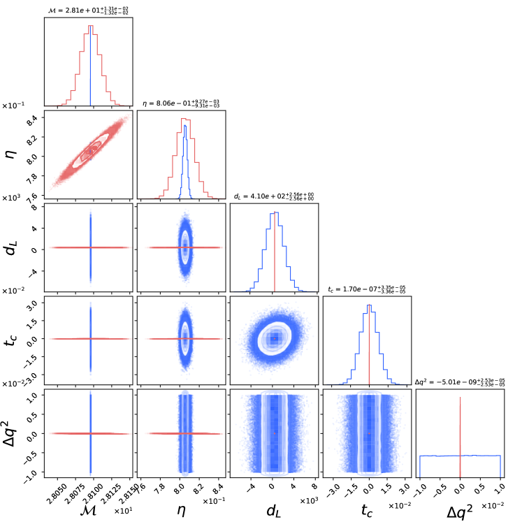
Figure 2: Parameter constraints for a GW150914-like event, i.e., $m_{1}=36M_{\odot}$, $m_{2}=29M_{\odot}$ and $d_{L}=410{\rm Mpc}$, obtained with mHz band (blue) and LVK band (red) observations. When calculating the Fisher information matrix, we assume the presence of a spin-0 field with $f_{\mu}=1{\rm Hz}$.

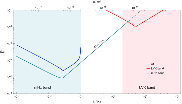
Figure 3: Discrimination on the spin of massive fields. The blue (red) lines show the difference between the spin-0 and the spin-1 field in GW phase, $\Delta\Psi\equiv\left|\Psi_{\rm MF}^{s=0}-\Psi_{\rm MF}^{s=1}\right|$, assuming a GW150914-like event observed in mHz (LVK) band. The green lines show the difference between the spin-0 and the spin-1 field in merger time $\Delta t$. The green region shows the parameter space where the detectability on the spin of the field can be improved by multi-band observations.

As demonstrated previously, observations in the mHz band alone can improve the detectability on massive fields, but only if for fields with $f_{\mu}<0.1{\rm Hz}$. Nevertheless, fields with $f_{\mu}>0.1{\rm Hz}$ can still affect the later binary evolution and accelerate orbital decay while observations in the mHz band can forecast the merger time with an accuracy of ${\cal O}(1)$ second. With a multi-band observation such that the binary is also observed later in the LVK band, the merger time forecasted by the mHz observations can be tested in the LVK band, providing an additional constraint on the dipole radiation induced by the massive fields. In Fig. 2, we consider a GW150914-like event, and estimate the constraints of the waveform parameters assuming there is a spin-0 field with $f_{\mu}=1{\rm Hz}$. Given the mass of the field, LVK band observation can probe the field if $|\Delta q|>10^{-2}$, while the mHz band observation alone cannot probe the filed at all. For the other parameters, observation in LVK band does better measurement on distance and merger time, while observation in mHz band does better measurement on masses. In particular, the mHz band can measure the merger time with an accuracy of $0.03s$ at $90\%$ confidence level.

Assuming $|\Delta q|\ll 1$, the merger time in the presence of dipole radiation will be earlier than that in GR by amount of

$$\Delta t \simeq \int_{f_{\mu}}^{f_{c}}\mathrm{d}f\left(\frac{P_{\rm MF}}{P_{\rm GR}^{2}}\right)\left(\frac{\mathrm{d}E}{\mathrm{d}f}\right)$$ (21)

$$\sim \frac{5}{3072}\Delta q^{2}\nu^{-1}\left(\pi Mf_{\mu}\right)^{-10/3}\,.$$ (22)

By requiring $\Delta t<1{\rm s}$, we find a constraint of

$$|\Delta q|<10^{-4}\left(\frac{\nu}{0.25}\right)^{1/2}\left(\frac{M}{60M_{\odot}}\right)^{5/3}\left(\frac{f_{\mu}}{1{\rm Hz}}\right)^{5/3}\,,$$ (23)

for $0.1{\rm Hz}<f_{\mu}<2{\rm Hz}$. In Fig. 1, we show the constraints on $|\Delta q|$ for fields with different masses by requiring $\Delta t<0.03{\rm s}$, assuming a multi-band observation of GW150914-like event. Comparing to the single band observations, we find that the multi-band observation indeed improves the detectability on $\Delta q$ by filling the gap between the mHz and the LVK bands.

Beside improving detectability of the massive fields, multi-band observation can further distinguish spin-0 fields from spin-1 fields. With observations in the LVK band or in the mHz band alone, we expect to distinguish the fields if they could induce ${\cal O}(1)$ difference in GW phase, namely $\left|\Psi_{\rm MF}^{s=0}-\Psi_{\rm MF}^{s=1}\right|\sim{\cal O}(1)$. Given Eq. (5), waveforms of spin-0 and spin-1 field differ notably only when the dipole radiation just turns on. Therefore, if $\mu\ll\Omega$ during the single band observation, one cannot distinguish whether the dipole radiation is caused by a spin-0 or spin-1 field, cf. Eq. (5), even with a nontrivial measurement of $\Delta q$. With multi-band observations, one can further infer whether the dipole radiation observed in the LVK band is from a spin-0 or spin-1 field by examine the merger time. Considering the GW150914-like event, Fig. 3 shows the GW phase difference for observations in the LVK and the mHz band, as well as the difference in merger time $\Delta t=|t_{c}^{s=0}-t_{c}^{s=1}|$, from which we can conclude that multi-band observations can distinguish the spin of the fields in some of the parameter space where the single-band observation cannot.

V Conclusion and Discussion

In this work, we investigate the prospect of probing massive fields with space borne detectors that target GWs in the mHz band. We consider the dipole radiation from generic massive spin-0 and spin-1 fields, calculate their imprints on the inspiral waveform and estimate the detachability on the fields. We demonstrate the detectability on the effective charge difference $|\Delta q|$ of LISA by calculating the Fisher information matrix. We find that LISA can constrain $|\Delta q|$ down to $10^{-6}$ for fields with mass below $3\times 10^{-17}{\rm eV}$, given a 4-year observation of a GW150914-like binary.

We further emphasis the implication of multi-band observations on probing new massive fields. We show that multi-band observation of a GW150914-like binary can improve the detectability on $\Delta q$ by at most 3 orders of magnitude for spin-0 and spin-1 fields with mass ranging from $10^{-16}{\rm eV}$ to $10^{-15}{\rm eV}$. Multi-band observation can further distinguish the spin of the fields in such mass range, where the spin of the field cannot be identified with single-band observations even if a non-trivial $\Delta q$ is detected.

Our multi-band detection strategy mainly depends on the measurement of merger time, which could in principle be affected by other beyond GR effects, such as modification of GW propagation speed. We expect such degeneracy can be break by considering multiple multi-band events, because effects from modification of GW speed depends on the distance of the sources while effects from massive fields should depends on the intrinsic parameters of the merger binaries. We shall leave this topic for future investigation.

Appendix A Corrections on GW phase

In this appendix, we show the explicit expressions for the corrections on the GW phase in the TaylorF2 waveform. As stated in the main text, the waveform template in frequency domain is

$$h(f)\simeq H(f)\exp\left[i\Psi(f)\right]\,,$$ (24)

where $\Psi(f)=2\pi ft-\phi-\tfrac{\pi}{4}$ is the GW phase, and is calculated under the stationary phase approximation,

$$t(f) = t_{c}-\int_{f_{c}}^{f}\frac{1}{P}\left(\frac{dE}{df^{\prime}}\right)\mathrm{d}f^{\prime}\,,$$ (25)

$$\phi(f) = \phi_{c}-\int_{f_{c}}^{f}\frac{2\pi f^{\prime}}{P}\left(\frac{dE}{df^{\prime}}\right)\mathrm{d}f^{\prime}\,.$$ (26)

Here $E$ and $P$ are the binding energy and total radiation power of the binary system, while $t_{c}$ and $\phi_{c}$ are the time and phase at merger. In the presence of a massive field, the total radiation power $P=P_{\rm GR}+P_{\rm MF}$. Assuming $|\Delta q|\ll 1$, we have $P_{\rm MF}\ll P_{\rm GR}$, and hence $t(f)\approx t_{\rm{GR}}(f)+t_{\rm{MF}}(f)$ and $\phi(f)\approx\phi_{\rm{GR}}(f)+\phi_{\rm{MF}}(f)$ with

$$t_{\rm{MF}}(f) =\int\frac{P_{\rm{MF}}}{{P_{\mathrm{GR}}^{2}}}\frac{\mathrm{d}E}{\mathrm{d}\Omega}\mathrm{d}\Omega\,,$$ (27)

$$\phi_{\rm{MF}}(f) =\int^{f}_{f_{c}}\frac{2\pi fP_{\rm{MF}}}{{P_{\mathrm{GR}}^{2}}}(\frac{\mathrm{d}E}{\mathrm{d}f})\mathrm{d}f\,.$$ (28)

For spin-0 field, we have

$$t_{\rm{MF}}^{s=0}(f) =\frac{3{f_{\mu}}^{2}}{19f^{\frac{16}{3}}_{c}}\sqrt{\frac{1-\frac{{f_{\mu}}^{2}}{f^{2}_{c}}}{1-\frac{f^{2}_{c}}{{f_{\mu}}^{2}}}}\times{}_{2}F_{1}\left(-\frac{19}{6},-\frac{3}{2};-\frac{13}{6};\frac{f^{2}_{c}}{{f_{\mu}}^{2}}\right)$$

$$-\frac{3{f_{\mu}}^{2}}{19f^{\frac{16}{3}}}\sqrt{\frac{1-\frac{{f_{\mu}}^{2}}{f^{2}}}{1-\frac{f^{2}}{{f_{\mu}}^{2}}}}\times{}_{2}F_{1}\left(-\frac{19}{6},-\frac{3}{2};-\frac{13}{6};\frac{f^{2}}{{f_{\mu}}^{2}}\right)\,,$$ (29)

$$\phi_{\rm{MF}}^{s=0}(f) =\frac{3{f_{\mu}}^{2}}{16f^{\frac{13}{3}}_{c}}\sqrt{\frac{1-\frac{{f_{\mu}}^{2}}{f^{2}_{c}}}{1-\frac{f^{2}_{c}}{{f_{\mu}}^{2}}}}\times{}_{2}F_{1}\left(-\frac{8}{3},-\frac{3}{2};-\frac{5}{3};\frac{f^{2}_{c}}{{f_{\mu}}^{2}}\right)$$

$$-\frac{3{f_{\mu}}^{2}}{16f^{\frac{13}{3}}}\sqrt{\frac{1-\frac{{f_{\mu}}^{2}}{f^{2}}}{1-\frac{f^{2}}{{f_{\mu}}^{2}}}}\times{}_{2}F_{1}\left(-\frac{8}{3},-\frac{3}{2};-\frac{5}{3};\frac{f^{2}}{{f_{\mu}}^{2}}\right)\,.$$ (30)

For spin-1 field, we have

$$t_{\rm{MF}}^{s=1}(f) =\frac{3}{494f^{16/3}_{c}}\sqrt{\frac{1-\frac{{f_{\mu}}^{2}}{f^{2}_{c}}}{1-\frac{f^{2}_{c}}{{f_{\mu}}^{2}}}}\times\left[13\sqrt{1-\frac{f^{2}_{c}}{{f_{\mu}}^{2}}}(f^{2}_{c}-{f_{\mu}}^{2})\right.$$

$$\quad\left.-48f^{2}_{c}\,{}_{2}F_{1}\left(-\frac{13}{6},-\frac{1}{2};-\frac{7}{6};\frac{f^{2}_{c}}{{f_{\mu}}^{2}}\right)\right]$$

$$-\frac{3}{494f^{16/3}}\sqrt{\frac{1-\frac{{f_{\mu}}^{2}}{f^{2}}}{1-\frac{f^{2}}{{f_{\mu}}^{2}}}}\times\left[13\sqrt{1-\frac{f^{2}}{{f_{\mu}}^{2}}}(f^{2}-{f_{\mu}}^{2})\right.$$

$$\quad\left.-48f^{2}\,_{2}F_{1}\left(-\frac{13}{6},-\frac{1}{2};-\frac{7}{6};\frac{f^{2}}{{f_{\mu}}^{2}}\right)\right]\,,$$ (31)

$$\phi_{\rm{MF}}^{s=1}(f) =\frac{3}{320f^{13/3}_{c}}\sqrt{\frac{1-\frac{{f_{\mu}}^{2}}{f^{2}_{c}}}{1-\frac{f^{2}_{c}}{{f_{\mu}}^{2}}}}\times\left[10\sqrt{1-\frac{f^{2}_{c}}{{f_{\mu}}^{2}}}(f^{2}_{c}-{f_{\mu}}^{2})\right.$$

$$\quad\left.-39f^{2}_{c}\,{}_{2}F_{1}\left(-\frac{5}{3},-\frac{1}{2};-\frac{2}{3};\frac{f^{2}_{c}}{{f_{\mu}}^{2}}\right)\right]$$

$$-\frac{3}{320f^{16/3}}\sqrt{\frac{1-\frac{{f_{\mu}}^{2}}{f^{2}}}{1-\frac{f^{2}}{{f_{\mu}}^{2}}}}\times\left[10\sqrt{1-\frac{f^{2}}{{f_{\mu}}^{2}}}(f^{2}-{f_{\mu}}^{2})\right.$$

$$\quad\left.-39f^{2}\,_{2}F_{1}\left(-\frac{5}{3},-\frac{1}{2};-\frac{2}{3};\frac{f^{2}}{{f_{\mu}}^{2}}\right)\right]\,.$$ (32)

The total correction on the GW phase is

$$\Psi_{\rm MF}=2\pi ft_{\rm{MF}}(f)-\phi_{\rm{MF}}(f)\,.$$ (33)

References

- Dima et al. [2020] A. Dima, E. Barausse, N. Franchini, and T. P. Sotiriou, Spin-induced black hole spontaneous scalarization, Phys. Rev. Lett. 125, 231101 (2020), arXiv:2006.03095 [gr-qc] .
- Herdeiro et al. [2021] C. A. R. Herdeiro, E. Radu, H. O. Silva, T. P. Sotiriou, and N. Yunes, Spin-induced scalarized black holes, Phys. Rev. Lett. 126, 011103 (2021), arXiv:2009.03904 [gr-qc] .
- Dolan [2007] S. R. Dolan, Instability of the massive Klein-Gordon field on the Kerr spacetime, Phys. Rev. D 76, 084001 (2007), arXiv:0705.2880 [gr-qc] .
- Percival and Dolan [2020] J. Percival and S. R. Dolan, Quasinormal modes of massive vector fields on the Kerr spacetime, Phys. Rev. D 102, 104055 (2020), arXiv:2008.10621 [gr-qc] .
- Garcia-Saenz et al. [2021] S. Garcia-Saenz, A. Held, and J. Zhang, Destabilization of Black Holes and Stars by Generalized Proca Fields, Phys. Rev. Lett. 127, 131104 (2021), arXiv:2104.08049 [gr-qc] .
- Damour and Esposito-Farese [1993] T. Damour and G. Esposito-Farese, Nonperturbative strong field effects in tensor - scalar theories of gravitation, Phys. Rev. Lett. 70, 2220 (1993).
- Doneva and Yazadjiev [2022] D. D. Doneva and S. S. Yazadjiev, Beyond the spontaneous scalarization: New fully nonlinear mechanism for the formation of scalarized black holes and its dynamical development, Phys. Rev. D 105, L041502 (2022), arXiv:2107.01738 [gr-qc] .
- Sotiriou and Zhou [2014] T. P. Sotiriou and S.-Y. Zhou, Black hole hair in generalized scalar-tensor gravity, Phys. Rev. Lett. 112, 251102 (2014), arXiv:1312.3622 [gr-qc] .
- Silva et al. [2018] H. O. Silva, J. Sakstein, L. Gualtieri, T. P. Sotiriou, and E. Berti, Spontaneous scalarization of black holes and compact stars from a Gauss-Bonnet coupling, Phys. Rev. Lett. 120, 131104 (2018), arXiv:1711.02080 [gr-qc] .
- Hook and Huang [2018] A. Hook and J. Huang, Probing axions with neutron star inspirals and other stellar processes, JHEP 06, 036, arXiv:1708.08464 [hep-ph] .
- Chen et al. [2020] Y. Chen, J. Shu, X. Xue, Q. Yuan, and Y. Zhao, Probing Axions with Event Horizon Telescope Polarimetric Measurements, Phys. Rev. Lett. 124, 061102 (2020), arXiv:1905.02213 [hep-ph] .
- Chen et al. [2022] Y. Chen, Y. Liu, R.-S. Lu, Y. Mizuno, J. Shu, X. Xue, Q. Yuan, and Y. Zhao, Stringent axion constraints with Event Horizon Telescope polarimetric measurements of M87∗, Nature Astron. 6, 592 (2022), arXiv:2105.04572 [hep-ph] .
- Abbott et al. [2016] B. P. Abbott et al. (LIGO Scientific, Virgo), Tests of general relativity with GW150914, Phys. Rev. Lett. 116, 221101 (2016), [Erratum: Phys.Rev.Lett. 121, 129902 (2018)], arXiv:1602.03841 [gr-qc] .
- Abbott et al. [2019a] B. P. Abbott et al. (LIGO Scientific, Virgo), Tests of General Relativity with GW170817, Phys. Rev. Lett. 123, 011102 (2019a), arXiv:1811.00364 [gr-qc] .
- Abbott et al. [2019b] B. P. Abbott et al. (LIGO Scientific, Virgo), Tests of General Relativity with the Binary Black Hole Signals from the LIGO-Virgo Catalog GWTC-1, Phys. Rev. D 100, 104036 (2019b), arXiv:1903.04467 [gr-qc] .
- Abbott et al. [2021a] R. Abbott et al. (LIGO Scientific, Virgo), Tests of general relativity with binary black holes from the second LIGO-Virgo gravitational-wave transient catalog, Phys. Rev. D 103, 122002 (2021a), arXiv:2010.14529 [gr-qc] .
- Abbott et al. [2021b] R. Abbott et al. (LIGO Scientific, VIRGO, KAGRA), Tests of General Relativity with GWTC-3, (2021b), arXiv:2112.06861 [gr-qc] .
- Yunes et al. [2016] N. Yunes, K. Yagi, and F. Pretorius, Theoretical Physics Implications of the Binary Black-Hole Mergers GW150914 and GW151226, Phys. Rev. D 94, 084002 (2016), arXiv:1603.08955 [gr-qc] .
- Wang et al. [2022] Y.-F. Wang, S. M. Brown, L. Shao, and W. Zhao, Tests of gravitational-wave birefringence with the open gravitational-wave catalog, Phys. Rev. D 106, 084005 (2022), arXiv:2109.09718 [astro-ph.HE] .
- Niu et al. [2022] R. Niu, T. Zhu, and W. Zhao, Testing Lorentz invariance of gravity in the Standard-Model Extension with GWTC-3, JCAP 12, 011, arXiv:2202.05092 [gr-qc] .
- Zhu et al. [2023] T. Zhu, W. Zhao, J.-M. Yan, C. Gong, and A. Wang, Tests of modified gravitational wave propagations with gravitational waves, (2023), arXiv:2304.09025 [gr-qc] .
- Lin et al. [2024] C. Lin, T. Zhu, R. Niu, and W. Zhao, Constraining the Modified Friction in Gravitational Wave Propagation with Precessing Black Hole Binaries, (2024), arXiv:2404.11245 [gr-qc] .
- Sesana [2016] A. Sesana, Prospects for Multiband Gravitational-Wave Astronomy after GW150914, Phys. Rev. Lett. 116, 231102 (2016), arXiv:1602.06951 [gr-qc] .
- Vitale [2016] S. Vitale, Multiband Gravitational-Wave Astronomy: Parameter Estimation and Tests of General Relativity with Space- and Ground-Based Detectors, Phys. Rev. Lett. 117, 051102 (2016), arXiv:1605.01037 [gr-qc] .
- Yunes and Pretorius [2009] N. Yunes and F. Pretorius, Fundamental Theoretical Bias in Gravitational Wave Astrophysics and the Parameterized Post-Einsteinian Framework, Phys. Rev. D 80, 122003 (2009), arXiv:0909.3328 [gr-qc] .
- Carson and Yagi [2020a] Z. Carson and K. Yagi, Multi-band gravitational wave tests of general relativity, Class. Quant. Grav. 37, 02LT01 (2020a), arXiv:1905.13155 [gr-qc] .
- Carson and Yagi [2020b] Z. Carson and K. Yagi, Parametrized and inspiral-merger-ringdown consistency tests of gravity with multiband gravitational wave observations, Phys. Rev. D 101, 044047 (2020b), arXiv:1911.05258 [gr-qc] .
- Gupta et al. [2020] A. Gupta, S. Datta, S. Kastha, S. Borhanian, K. G. Arun, and B. S. Sathyaprakash, Multiparameter tests of general relativity using multiband gravitational-wave observations, Phys. Rev. Lett. 125, 201101 (2020), arXiv:2005.09607 [gr-qc] .
- Datta et al. [2021] S. Datta, A. Gupta, S. Kastha, K. G. Arun, and B. S. Sathyaprakash, Tests of general relativity using multiband observations of intermediate mass binary black hole mergers, Phys. Rev. D 103, 024036 (2021), arXiv:2006.12137 [gr-qc] .
- Barausse et al. [2016] E. Barausse, N. Yunes, and K. Chamberlain, Theory-Agnostic Constraints on Black-Hole Dipole Radiation with Multiband Gravitational-Wave Astrophysics, Phys. Rev. Lett. 116, 241104 (2016), arXiv:1603.04075 [gr-qc] .
- Chamberlain and Yunes [2017] K. Chamberlain and N. Yunes, Theoretical Physics Implications of Gravitational Wave Observation with Future Detectors, Phys. Rev. D 96, 084039 (2017), arXiv:1704.08268 [gr-qc] .
- Liu et al. [2020a] C. Liu, L. Shao, J. Zhao, and Y. Gao, Multiband Observation of LIGO/Virgo Binary Black Hole Mergers in the Gravitational-wave Transient Catalog GWTC-1, Mon. Not. Roy. Astron. Soc. 496, 182 (2020a), arXiv:2004.12096 [astro-ph.HE] .
- Zhao et al. [2021] J. Zhao, L. Shao, Y. Gao, C. Liu, Z. Cao, and B.-Q. Ma, Probing dipole radiation from binary neutron stars with ground-based laser-interferometer and atom-interferometer gravitational-wave observatories, Phys. Rev. D 104, 084008 (2021), arXiv:2106.04883 [gr-qc] .
- Harry and Noller [2022] I. Harry and J. Noller, Probing the speed of gravity with LVK, LISA, and joint observations, Gen. Rel. Grav. 54, 133 (2022), arXiv:2207.10096 [gr-qc] .
- Baker et al. [2023] T. Baker, E. Barausse, A. Chen, C. de Rham, M. Pieroni, and G. Tasinato, Testing gravitational wave propagation with multiband detections, JCAP 03, 044, arXiv:2209.14398 [gr-qc] .
- Gnocchi et al. [2019] G. Gnocchi, A. Maselli, T. Abdelsalhin, N. Giacobbo, and M. Mapelli, Bounding alternative theories of gravity with multiband GW observations, Phys. Rev. D 100, 064024 (2019), arXiv:1905.13460 [gr-qc] .
- Anderson et al. [2019] D. Anderson, P. Freire, and N. Yunes, Binary pulsar constraints on massless scalar–tensor theories using Bayesian statistics, Class. Quant. Grav. 36, 225009 (2019), arXiv:1901.00938 [gr-qc] .
- Kumar Poddar et al. [2020] T. Kumar Poddar, S. Mohanty, and S. Jana, Constraints on ultralight axions from compact binary systems, Phys. Rev. D 101, 083007 (2020), arXiv:1906.00666 [hep-ph] .
- Seymour and Yagi [2020] B. C. Seymour and K. Yagi, Probing massive scalar and vector fields with binary pulsars, Phys. Rev. D 102, 104003 (2020), arXiv:2007.14881 [gr-qc] .
- Poddar et al. [2023] T. K. Poddar, A. Ghoshal, and G. Lambiase, Listening to dark sirens from gravitational waves:\itCombined effects of fifth force, ultralight particle radiation, and eccentricity, (2023), arXiv:2302.14513 [hep-ph] .
- Zhang et al. [2023] C. Zhang, N. Dai, Q. Gao, Y. Gong, T. Jiang, and X. Lu, Detecting new fundamental fields with pulsar timing arrays, Phys. Rev. D 108, 104069 (2023), arXiv:2307.01093 [gr-qc] .
- Toubiana et al. [2020] A. Toubiana, S. Marsat, E. Barausse, S. Babak, and J. Baker, Tests of general relativity with stellar-mass black hole binaries observed by LISA, Phys. Rev. D 101, 104038 (2020), arXiv:2004.03626 [gr-qc] .
- Maselli et al. [2020] A. Maselli, N. Franchini, L. Gualtieri, and T. P. Sotiriou, Detecting scalar fields with Extreme Mass Ratio Inspirals, Phys. Rev. Lett. 125, 141101 (2020), arXiv:2004.11895 [gr-qc] .
- Liu et al. [2020b] T. Liu, W. Zhao, and Y. Wang, Gravitational waveforms from the quasicircular inspiral of compact binaries in massive Brans-Dicke theory, Phys. Rev. D 102, 124035 (2020b), arXiv:2007.10068 [gr-qc] .
- Gao et al. [2023] Q. Gao, Y. You, Y. Gong, C. Zhang, and C. Zhang, Testing alternative theories of gravity with space-based gravitational wave detectors, Phys. Rev. D 108, 024027 (2023), arXiv:2212.03789 [gr-qc] .
- Sagunski et al. [2018] L. Sagunski, J. Zhang, M. C. Johnson, L. Lehner, M. Sakellariadou, S. L. Liebling, C. Palenzuela, and D. Neilsen, Neutron star mergers as a probe of modifications of general relativity with finite-range scalar forces, Phys. Rev. D 97, 064016 (2018), arXiv:1709.06634 [gr-qc] .
- Huang et al. [2019] J. Huang, M. C. Johnson, L. Sagunski, M. Sakellariadou, and J. Zhang, Prospects for axion searches with Advanced LIGO through binary mergers, Phys. Rev. D 99, 063013 (2019), arXiv:1807.02133 [hep-ph] .
- Kuntz et al. [2019] A. Kuntz, F. Piazza, and F. Vernizzi, Effective field theory for gravitational radiation in scalar-tensor gravity, JCAP 05, 052, arXiv:1902.04941 [gr-qc] .
- Diedrichs et al. [2023] R. F. Diedrichs, D. Schmitt, and L. Sagunski, Binary Systems in Massive Scalar-Tensor Theories: Next-to-Leading Order Gravitational Waveform from Effective Field Theory, (2023), arXiv:2311.04274 [gr-qc] .
- Zhang et al. [2021] J. Zhang, Z. Lyu, J. Huang, M. C. Johnson, L. Sagunski, M. Sakellariadou, and H. Yang, First Constraints on Nuclear Coupling of Axionlike Particles from the Binary Neutron Star Gravitational Wave Event GW170817, Phys. Rev. Lett. 127, 161101 (2021), arXiv:2105.13963 [hep-ph] .
- Grant et al. [2023] A. M. Grant, A. Saffer, L. C. Stein, and S. Tahura, Gravitational-wave energy and other fluxes in ghost-free bigravity, Phys. Rev. D 107, 044041 (2023), arXiv:2208.02123 [gr-qc] .
- Krause et al. [1994] D. Krause, H. T. Kloor, and E. Fischbach, Multipole radiation from massive fields: Application to binary pulsar systems, Phys. Rev. D 49, 6892 (1994).
- Alsing et al. [2012] J. Alsing, E. Berti, C. M. Will, and H. Zaglauer, Gravitational radiation from compact binary systems in the massive Brans-Dicke theory of gravity, Phys. Rev. D 85, 064041 (2012), arXiv:1112.4903 [gr-qc] .
- Yagi [2012] K. Yagi, A New constraint on scalar Gauss-Bonnet gravity and a possible explanation for the excess of the orbital decay rate in a low-mass X-ray binary, Phys. Rev. D 86, 081504 (2012), arXiv:1204.4524 [gr-qc] .
- Yagi et al. [2016] K. Yagi, L. C. Stein, and N. Yunes, Challenging the Presence of Scalar Charge and Dipolar Radiation in Binary Pulsars, Phys. Rev. D 93, 024010 (2016), arXiv:1510.02152 [gr-qc] .
- Zhang et al. [2020] C. Zhang, X. Zhao, A. Wang, B. Wang, K. Yagi, N. Yunes, W. Zhao, and T. Zhu, Gravitational waves from the quasicircular inspiral of compact binaries in Einstein-aether theory, Phys. Rev. D 101, 044002 (2020), [Erratum: Phys.Rev.D 104, 069905 (2021)], arXiv:1911.10278 [gr-qc] .
- Niu et al. [2019] R. Niu, X. Zhang, T. Liu, J. Yu, B. Wang, and W. Zhao, Constraining Screened Modified Gravity by Space-borne Gravitational-wave Detectors, Astrophys. J. 890, 163 (2019), arXiv:1910.10592 [gr-qc] .
- Niu et al. [2021] R. Niu, X. Zhang, B. Wang, and W. Zhao, Constraining Scalar-tensor Theories Using Neutron Star–Black Hole Gravitational Wave Events, Astrophys. J. 921, 149 (2021), arXiv:2105.13644 [gr-qc] .
- Liu et al. [2023] T. Liu, Y. Wang, and W. Zhao, Gravitational waveforms from the inspiral of compact binaries in the Brans-Dicke theory in an expanding Universe, Phys. Rev. D 108, 024006 (2023), arXiv:2205.03704 [gr-qc] .
- Li et al. [2024] Z. Li, J. Qiao, T. Liu, R. Niu, S. Hou, T. Zhu, and W. Zhao, Gravitational radiation from eccentric binary black hole system in dynamical Chern-Simons gravity, JCAP 05, 073, arXiv:2309.05991 [gr-qc] .
- [61] Updated advanced ligo design curve, https://dcc.ligo.org/LIGO-T1800044-v3/public.
- Robson et al. [2019] T. Robson, N. J. Cornish, and C. Liu, The construction and use of LISA sensitivity curves, Class. Quant. Grav. 36, 105011 (2019), arXiv:1803.01944 [astro-ph.HE] .