Deflection of light by wormholes and its shadow due to dark matter within modified symmetric teleparallel gravity formalism

Abstract

We explore the possibility of traversable wormhole formation in the dark matter halos in the context of $f(Q)$ gravity. We obtain the exact wormhole solutions with anisotropic matter source based on the Bose-Einstein condensate, Navarro-Frenk-White, and pseudo-isothermal matter density profiles. Notably, we present a novel wormhole solution supported by these dark matters using the expressions for the density profile and rotational velocity along with the modified field equations to calculate the redshift and shape functions of the wormholes. With a particular set of parameters, we demonstrate that our proposed wormhole solutions fulfill the flare-out condition against an asymptotic background. Additionally, we examine the energy conditions, focusing on the null energy conditions at the wormhole’s throat, providing a graphical representation of the feasible and negative regions. Our study also examines the wormhole’s shadow in the presence of various dark matter models, revealing that higher central densities result in a shadow closer to the throat, whereas lower values have the opposite effect. Moreover, we explore the deflection of light when it encounters these wormholes, particularly noting that light deflection approaches infinity at the throat, where the gravitational field is extremely strong.

Keywords: Wormhole shadow, gravitational lensing, energy conditions, $f(Q)$ gravity.

I Introduction

The theory of general relativity and other extended theories of gravity present the possibility of space-time hosting complicated structures, such as wormholes. These wormholes are tunnel-like passages that connect disparate or distant regions of space. Within the General Relativity (GR) framework, black holes and wormholes stand out as fascinating astrophysical phenomena. While researchers have confirmed the existence of black holes in [1, 2, 3], the presence of wormholes remains an ongoing investigation. The concept of wormholes traces back to the pioneering work of Einstein and Rosen, who proposed the first wormhole solution known as the Einstein-Rosen bridge [4]. Wormholes gained renewed interest when Ellis [5] introduced a novel solution incorporating a spherically symmetric configuration of Einstein’s equations, incorporating a massless scalar field with ghost properties. Morris and Thorne [6] later demonstrated that these Ellis wormholes could indeed be traversable, potentially facilitating rapid travel through space and even raising the possibility of time travel. Notably, such wormhole models do not feature singularities or horizons, and their tidal forces are deemed survivable for humans. Additionally, Morris and Thorne [6] indicated that these wormhole solutions would violate the null energy conditions, necessitating the presence of exotic matter. This exotic matter, disobeying energy conditions, exhibits characteristics that challenge established laws of physics, including the potential for particles to possess negative mass. An extensive investigation has been conducted into the presence of wormholes in [7], while numerous scholars have explored the stability of traversable wormholes. Notably, Shinkai and Hayward [8] demonstrated the instability exhibited by Ellis wormholes through numerical simulations. Since the inception of the traversable wormhole concept, researchers have been fascinated by the possibility of constructing such passages using ordinary matter. Recent research indicates that within modified gravity theories, it may be feasible to construct wormholes composed of ordinary matter that satisfy all energy conditions [9]. However, in the process of utilizing modified gravity to create wormholes, although the matter involved may be ordinary, the effective geometric matter, which serves as the source of modified gravity, could still violate the standard null energy condition. Several investigations have been done on wormhole configurations that do not demand exotic matter [10, 11, 12, 13, 14, 15, 16, 17].
The formulation of $f(Q)$ gravity arises from the development of novel classes of modified gravity, originating from symmetric teleparallel gravity based on the non-metricity scalar Q. Essentially, $f(Q)$ gravity serves as an extension of symmetric teleparallel gravity, which operates within a framework of a flat connection with vanishing torsion. Jimenez et al. [18] introduced a theoretical framework where curvature and torsion vanish, and gravity is attributed to non-metricity $Q$. This $f(Q)$ theory has demonstrated the capacity to explain the Universe’s accelerated expansion with a statistical precision comparable to renowned modified gravities [19]. The cosmological implications of $f(Q)$ gravity have been extensively explored in [20, 21, 22]. Harko and his collaborators [23] employed $f(Q)$ gravity to study cosmological evolutions and related phenomena. Additionally, Anagnostopoulos et al. [24] employed Big Bang Nucleosynthesis formalism and observational data to constrain various classes of $f(Q)$ models. Numerous other researchers have contributed to investigating cosmological aspects within the framework of $f(Q)$ gravity [25, 26, 27, 28, 29].
Investigations into black hole solutions within the framework of $f(Q)$ gravity have been conducted in Refs. [30, 31, 32]. Additionally, the formation and properties of compact stars resulting from gravitational decoupling in $f(Q)$ gravity theory have been examined in [33]. Sokoliuk et al. [34] studied Buchdahl quark stars within the context of the $f(Q)$ theory. Spherically symmetric configurations within $f(Q)$ gravity have been investigated in [19]. They have examined with a specific polynomial expression, such as $f(Q)=Q+\alpha Q^{2}$, while employing polytropic Equations of State (EoS) to characterize internal spherically symmetric configurations. Wang et al. [35] presented static and spherically symmetric solutions incorporating an anisotropic fluid for general $f(Q)$ gravity formulations. Calza and Sebastiani [36] analyzed a class of topological static spherically symmetric vacuum solutions with constant non-metricity within $f(Q)$ gravity. Further, Mustafa et al. [37] employed the Karmarkar conditions in the $f(Q)$ gravity formalism to derive wormhole solutions that adhere to Energy Conditions (ECs). Furthermore, investigations into wormhole geometries within the $f(Q)$ gravity framework have been carried out in [38], revealing that a linear model may require a minimal amount of exotic matter for a traversable wormhole. Additionally, Sharma et al. [39] explored wormhole solutions within symmetric teleparallel gravity, emphasizing specific shape and redshift functions within certain $f(Q)$ models that can yield solutions satisfying ECs in some regions of space-time. Recently, the Casimir wormhole and its GUP correction in the $f(Q)$ gravity framework have been examined in [40, 41]. Moreover, readers can also check some interesting works of literature related to astrophysical objects found in non-metricity-based modified theories of gravity (see Refs. [42, 43, 44, 45, 46, 47]).
The notion of dark matter, a mysterious form of matter containing approximately 25% of the Universe’s total matter content, emerges from observational predictions. Various candidates from particle physics and supersymmetric string theory, such as axions and weakly interacting massive particles, are considered compelling nominees for dark matter despite the absence of direct experimental confirmation. Nevertheless, indications of its presence are observed in phenomena such as galactic rotation curves [48], galaxy cluster dynamics [49], and cosmological observations of anisotropies in the cosmic microwave background as measured by PLANCK [50]. The literature [51, 52] explores considerations of traversable wormholes (TWs) within dark matter halos and galaxy formation regions, typically based on the Navarro-Frenk-White (NFW) profile [53] of matter distribution. Rahaman et al. [54] initially proposed the existence of potential wormholes in the outer regions of galactic halos based on the NFW density profile, extending their analysis to utilize the universal rotation curve (URC) dark matter model to derive analogous results within the central portion of the halo [52]. Also, dark matter, considered a non-relativistic matter describable by NFW and King profiles, is employed to construct wormholes [55]. Discrepancies between NFW halo velocity profiles and the observed dynamics of spiral galaxies remain unresolved, leading to modifications in the original NFW halo profiles within the $\Lambda$CDM scenario to align with observational data [56]. Additionally, it is shown that the presence of TWs in nature could be inferred through the study of scalar wave scattering [51].
In a recent study, Jusufi et al. [57] highlighted the potential formation of TW through the presence of a Bose-Einstein condensation dark matter (BEC-DM) halo. This BEC-DM model presents a more reasonable framework, particularly concerning the smaller scales of galaxies when compared to the Cold Dark Matter (CDM) model [58]. Notably, within the inner regions of galaxies, the interactions among dark matter particles are significantly vital, resulting in a deviation from cold dark matter behavior and rendering the density profile unsuitable. Consequently, the BEC-DM model indicates considerably lower dark matter densities in the central regions of galaxies compared to those projected by the NFW profile. Additionally, an alternative category of dark matter characterized by a pseudo isothermal (PI) profile, alongside the CDM and BEC-DM model, is associated with modifications to gravity, such as Modified Newtonian Dynamics (MOND) [59]. MOND [60, 61, 62] indicates that the discrepancies in mass within galactic systems arise not from dark matter but from deviations from standard dynamics at lower accelerations. In [63], Paul investigated the existence of TWs in the presence of MOND with or without a scalar field.
Gravitational lensing stands as an early useful exploration within the realm of general relativity, which was initially delved into by Einstein [64]. This phenomenon unfolds when a significantly massive celestial body bends incoming light, much like a lens, offering observers enhanced insights into the originating source. The interest in this area surged following the observed validation of light’s deflection, as indicated theoretically [65, 66]. Its scope extends beyond celestial bodies, opening avenues to probe into exoplanets, dark matter, and dark energy. A notable milestone was achieved with the first successful measurement of a white dwarf’s mass, Stein 2051 B, through astrometric microlensing [67]. An intriguing aspect of gravitational lensing is its potential to cause light to bend infinitely in unstable light rings, creating numerous relativistic images under strong lensing conditions [68, 69, 70]. This phenomenon, in both strong and weak forms, serves as a potent analytical tool for examining gravitational fields near various cosmic entities, including black holes and wormholes. Theoretical and astrophysical investigations have extensively applied gravitational lensing to study wormholes, reflecting its significance in contemporary research [71, 72, 73, 74, 75, 76, 77, 78, 79, 80].
Motivated by the above discussions, we have investigated wormhole solutions under different DM halo models in the context of $f(Q)$ gravity. The structure of this paper is outlined as follows: In section II, we present the basic formalism of $f(Q)$ gravity and the corresponding wormhole field equations under this gravity. We also discuss dark matter profiles and wormhole solutions under these models in section III. Later, in section IV, we present the analytical and graphical representations of the energy conditions of wormhole solutions. Furthermore, we examine wormhole shadows and deflection angles cast by wormholes in sections V and VI, respectively. Additionally, we present the geometry of the embedded wormhole space-time along with embedded diagrams in section VII. Finally, we conclude our discussions in the last section.

II Wormhole Field equations in $f(Q)$ gravity

In this section, we aim to introduce the fundamental layout of the wormhole theory and provide a brief review of the $f(Q)$ gravity formalism. We consider spherically symmetric static Morris-Thorne wormhole metric [6], defined by

$$ds^{2}=-e^{2\phi(r)}dt^{2}+\left(1-\frac{b(r)}{r}\right)^{-1}dr^{2}+r^{2}d\theta^{2}+r^{2}\text{sin}^{2}\theta d\Phi^{2},$$ (1)

where $b(r)$ and $\phi(r)$ represent the shape and redshift functions, respectively. The flaring-out condition is a key factor in determining whether a wormhole can be traversed. This condition is mathematically expressed as [6]

$$(b-b^{\prime}r)/b^{2}>0.$$ (2)

Specifically, at the wormhole’s throat, this formula simplifies the requirement that

$$b^{\prime}(r_{0})<1.$$ (3)

Additionally, for any point beyond the throat, i.e., $r>r_{0}$, the condition $1-\frac{b(r)}{r}>0$ must also be met. Further, the wormhole should be asymptotically flat, i.e.,

$$\frac{b(r)}{r}\rightarrow 0\,\,\,\,\text{as}\,\,\,r\rightarrow 0.$$ (4)

Also, for an event horizon-free, the redshift function must be finite everywhere.

Now, we will provide an overview of $f(Q)$ gravity, also known as symmetric teleparallel gravity, as initially proposed by Jimenez et al. [18]. The formulation of this gravity involves an action expressed as

$$\mathcal{S}=\int\frac{1}{2}\,f(Q)\sqrt{-g}\,d^{4}x+\int\mathcal{L}_{m}\,\sqrt{-g}\,d^{4}x\,,$$ (5)

where $f(Q)$ represents an arbitrary function of $Q$ and $\mathcal{L}_{m}$ denotes the matter Lagrangian density. $g$ corresponds to the determinant of the metric tensor $g_{\mu\nu}$.
Now, one can define the non-metricity tensor

$$Q_{\lambda\mu\nu}=\bigtriangledown_{\lambda}g_{\mu\nu}=\partial_{\lambda}g_{\mu\nu}-\Gamma^{\beta}_{\,\,\,\lambda\mu}g_{\beta\nu}-\Gamma^{\beta}_{\,\,\,\lambda\nu}g_{\mu\beta},$$ (6)

where, $\Gamma^{\beta}_{\,\,\,\mu\nu}$ is the metric affine connection.
Also, the superpotential is expressed by

$$P^{\alpha}\;_{\mu\nu}=\frac{1}{4}\left[-Q^{\alpha}\;_{\mu\nu}+2Q_{(\mu}\;^{\alpha}\;{}_{\nu)}+Q^{\alpha}g_{\mu\nu}-\tilde{Q}^{\alpha}g_{\mu\nu}\right.\\ \left.-\delta^{\alpha}_{(\mu}Q_{\nu)}\right],$$ (7)

where

$$Q_{\alpha}=Q_{\alpha}\;^{\mu}\;{}_{\mu},\;\tilde{Q}_{\alpha}=Q^{\mu}\;_{\alpha\mu}.$$ (8)

are two traces.
Further, the non-metricity scalar is presented by [18]

$$Q=-Q_{\alpha\mu\nu}\,P^{\alpha\mu\nu}.$$ (9)

In this context, the field equations are derived by varying the action (5) with respect to the metric tensor $g_{\mu\nu}$

$$\frac{2}{\sqrt{-g}}\bigtriangledown_{\gamma}\left(\sqrt{-g}\,f_{Q}\,P^{\gamma}\;_{\mu\nu}\right)+\frac{1}{2}g_{\mu\nu}f\\ +f_{Q}\left(P_{\mu\gamma i}\,Q_{\nu}\;^{\gamma i}-2\,Q_{\gamma i\mu}\,P^{\gamma i}\;_{\nu}\right)=-T_{\mu\nu},$$ (10)

where $f_{Q}=\frac{df}{dQ}$ and $T_{\mu\,\nu}$ is the energy-momentum tensor of the form

$$T_{\mu\nu}=-\frac{2}{\sqrt{-g}}\frac{\delta\left(\sqrt{-g}\,\mathcal{L}_{m}\right)}{\delta g^{\mu\nu}}.$$ (11)

Further, one can vary the action with respect to the connection and obtain the extra constraint

$$\bigtriangledown_{\mu}\bigtriangledown_{\nu}\left(\sqrt{-g}\,f_{Q}\,P^{\gamma}\;_{\mu\nu}\right)=0.$$ (12)

One can study this theory using a coincident gauge involving a specific coordinate choice. In this gauge, the connection disappears, and the non-metricity expressed in Eq. (6) can be simplified to the form

$$Q_{\lambda\mu\nu}=\partial_{\lambda}g_{\mu\nu}.$$ (13)

This simplification makes calculations easier since only the metric is considered a fundamental variable. However, it should be noted that the action is no longer diffeomorphism invariant in this case, except for standard GR, as stated in [81].
Now, we can obtain the non-metricity scalar for the metric (1) from Eq. (9)

$$Q=-\frac{2}{r}\left(1-\frac{b}{r}\right)\left(2\phi^{{}^{\prime}}+\frac{1}{r}\right).$$ (14)

Also, we assume the matter that is described by the anisotropic fluid which can be written in the form

$$T^{\mu}_{\nu}=\text{diag}[-\rho,\,P_{r},\,P_{t},\,P_{t}],$$ (15)

where $\rho$ represents the energy density. $P_{r}$ and $P_{t}$ denotes the radial and tangential pressure, respectively.
Now, the field equations for the metric (1) under anisotropic matter (15) within the framework of modified symmetric teleparallel gravity can be derived as

$$\left[\frac{1}{r}\left(-\frac{1}{r}+\frac{rb^{{}^{\prime}}+b}{r^{2}}-2\phi^{{}^{\prime}}\left(1-\frac{b}{r}\right)\right)\right]f_{Q}\\ -\frac{2}{r}\left(1-\frac{b}{r}\right)f_{QQ}Q^{{}^{\prime}}-\frac{f}{2}=-\rho,$$ (16)

$$\left[\frac{2}{r}\left(1-\frac{b}{r}\right)\left(2\phi^{{}^{\prime}}+\frac{1}{r}\right)-\frac{1}{r^{2}}\right]f_{Q}+\frac{f}{2}=-P_{r},$$ (17)

$$\left[\frac{1}{r}\left(\left(1-\frac{b}{r}\right)\left(\frac{1}{r}+\phi^{{}^{\prime}}\left(3+r\phi^{{}^{\prime}}\right)+r\phi^{{}^{\prime\prime}}\right)-\frac{rb^{{}^{\prime}}-b}{2r^{2}}\right.\right.\\ \left.\left.\left(1+r\phi^{{}^{\prime}}\right)\right)\right]f_{Q}+\frac{1}{r}\left(1-\frac{b}{r}\right)\left(1+r\phi^{{}^{\prime}}\right)f_{QQ}Q^{{}^{\prime}}\\ +\frac{f}{2}=-P_{t},$$ (18)

$$\frac{\cot{\theta}}{2}f_{QQ}Q^{{}^{\prime}}=0,$$ (19)

where ^′ represents $\frac{d}{dr}$. Now, looking at the off-diagonal component given in Eq. (19) gives the following relation

$$f_{QQ}=0\implies f(Q)=c_{0}+c_{1}Q,$$ (20)

where, $c_{0}$ and $c_{1}$ are constant. Therefore, we get the revised field equations as follows

$$\rho=\frac{c_{0}}{2}-\frac{c_{1}b^{\prime}}{r^{2}},$$ (21)

$$P_{r}=\frac{c_{1}\left(2r(b-r)\phi^{\prime}+b\right)}{r^{3}}-\frac{c_{0}}{2},$$ (22)

$$P_{t}=\frac{c_{1}\left(r\phi^{\prime}+1\right)\left(rb^{\prime}+2r(b-r)\phi^{\prime}-b\right)}{2r^{3}}\\ +\frac{c_{1}(b-r)\phi^{\prime\prime}}{r}-\frac{c_{0}}{2}.$$ (23)

Now, in the following sections, we shall study wormhole geometry under the effect of different dark matter models.

III Wormhole solutions due to dark matters

In this section, we shall try to find the wormhole shape function as well as the redshift function and discuss the necessary properties of a traversable wormhole under the effect of dark matter. For our study, we will consider three well-known dark matter models, Bose-Einstein condensate, Psudo Isothermal, and Navarro-Frenk-White.

III.1 Bose-Einstein condensate

This section presents the theory of Bose-Einstein Condensate (BEC) dark matter as outlined in [82]. It is worth noting that in a quantum system containing N interacting condensed bosons, the quantum state of these bosons can be effectively represented by a single-particle quantum state. The collective behavior of these interacting bosons, subject to an external potential $V_{ext}$, can be effectively described by the Hamiltonian [82]

$$\hat{H}=\int d\vec{r}\hat{\Psi}^{+}(\vec{r})\left[-\frac{\hbar}{2m}\bigtriangledown^{2}+V_{rot}\vec{r}+V_{ext}\vec{r}\right]\hat{\Psi}(\vec{r})\\ +\frac{1}{2}\int d\vec{r}d\vec{r}^{{}^{\prime}}\hat{\Psi}^{+}(\vec{r})\hat{\Psi}^{+}\vec{r}^{{}^{\prime}}V(\vec{r}-\vec{r}^{{}^{\prime}})\hat{\Psi}(\vec{r})\hat{\Psi}(\vec{r}^{{}^{\prime}}),$$ (24)

where $\hat{\Psi}(\vec{r})$ and $\hat{\Psi}^{+}(\vec{r})$ represent the boson field operators responsible for annihilating and creating a particle at the position $\vec{r}$, respectively. The term $V(\vec{r}-\vec{r}^{{}^{\prime}})$ denotes the two-body interatomic potential [83]. For this paper, we neglect the potential associated with the rotation of the condensate, thus setting $V_{rot}(\vec{r})=0$. Assuming $V_{ext}(\vec{r})$ to be the gravitational potential $V$, we satisfy the Poisson equation given by [82]

$$\bigtriangledown^{2}V=4\pi G\rho_{m},$$

Here, $\rho_{m}=m\rho$ represents the mass density within the BEC. By considering only the first approximation and disregarding the rotation of the BEC, i.e., $V_{rot}=0$, we can calculate the radius R of the BEC as [82]

$$R=\pi\sqrt{\frac{\hbar^{2}\alpha}{Gm^{3}}},$$ (25)

Here, $\alpha$, known as the scattering length, is linked to the scattering cross-section of particles within the condensate. Various estimations of the mass and scattering length of condensate dark matter particles exist in the literature. For instance, the scattering length $\alpha$, inferred from astrophysical observations of the Bullet Cluster, falls within the range of $10^{-7}$ $fm$, with the mass of the dark matter particle being approximately $\mu eV$ [84].

The following result is retrieved for the density distribution of the dark matter BEC [82]

$$\rho(r)=\rho_{s}\frac{\sin{kr}}{kr},$$ (26)

where $\rho_{s}$ denotes the central density of the condensate and $k=\sqrt{Gm^{3}/\hbar^{2}\alpha}$. The mass profile of the dark condensate galactic halo can be read as

$$M(r)=4\pi\int_{0}^{r}\rho(r)r^{2}dr.$$ (27)

and its solution is

$$M(r)=\frac{4\pi\rho_{s}}{k^{2}}r\left(\frac{\sin{kr}}{kr}-\cos{kr}\right).$$ (28)

From the above Eq. (28), we can obtain the tangential velocity of a test particle moving in the dark halo from the following relation

$$v_{t}^{2}(r)=G\,M(r)/r,$$ (29)

and hence

$$v_{t}^{2}(r)=\frac{4\pi G\rho_{s}}{k^{2}}\left(\frac{\sin{kr}}{kr}-\cos{kr}\right),$$ (30)

where $k=\pi/R$. For $r\rightarrow 0$, we have $v_{t}^{2}(r)\rightarrow 0$.

III.1.1 Finding solutions

Note that within the equatorial plane, the rotational velocity of a test particle in spherically symmetric space-time is defined by [82]

$$v_{t}^{2}(r)=r\,\phi^{{}^{\prime}}(r).$$ (31)

Inserting the Eq. (30) in the above relation (31), we have

$$\frac{4R^{2}\rho_{s}}{\pi}\left[\frac{\sin\left({\frac{\pi r}{R}}\right)}{\frac{\pi r}{R}}-\cos\left({\frac{\pi r}{R}}\right)\right]=r\,\phi^{{}^{\prime}}(r).$$ (32)

On solving, we find

$$\phi(r)=D_{1}-\frac{4\rho_{s}R^{3}\sin\left(\frac{\pi r}{R}\right)}{\pi^{2}r},$$ (33)

where $D_{1}$ is an integrating constant.
Now, we equate the density of the wormhole matter with the density of the BEC using Eqs. (21) and (26), it follows that

$$\frac{c_{0}}{2}-\frac{c_{1}b^{\prime}(r)}{r^{2}}=\frac{\rho_{s}R}{\pi r}\sin\left({\frac{\pi r}{R}}\right).$$ (34)

Solving for $b(r)$, we get

$$b(r)=\frac{\frac{1}{3}\pi c_{0}r^{3}-\frac{2\rho_{s}R^{3}\sin\left(\frac{\pi r}{R}\right)}{\pi^{2}}+\frac{2\rho_{s}rR^{2}\cos\left(\frac{\pi r}{R}\right)}{\pi}}{2\pi c_{1}}+c_{3}.$$ (35)

Now to find the integrating constant $c_{3}$, we impose the throat condition $b(r_{0})=r_{0}$

$$c_{3}=r_{0}-\frac{1}{2\pi c_{1}}\left[\frac{1}{3}\pi c_{0}r_{0}^{3}-\frac{2\rho_{s}R^{3}\sin\left(\frac{\pi r_{0}}{R}\right)}{\pi^{2}}\right.\\ \left.+\frac{2\rho_{s}R^{2}r_{0}\cos\left(\frac{\pi r_{0}}{R}\right)}{\pi}\right],$$ (36)

and hence the shape function $b(r)$ becomes

$$b(r)=\frac{1}{6c_{1}}\left[c_{0}r^{3}-c_{0}r_{0}^{3}+6c_{1}r_{0}\right.\\ \left.+\frac{1}{\pi^{3}}\left(6\rho_{s}R^{2}\left(-R\Lambda_{1}+\pi\Lambda_{2}\right)\right)\right],$$ (37)

where

$$\Lambda_{1}=\left(\sin\left(\frac{\pi r}{R}\right)-\sin\left(\frac{\pi r_{0}}{R}\right)\right),$$ (38)

$$\Lambda_{2}=r\cos\left(\frac{\pi r}{R}\right)-r_{0}\cos\left(\frac{\pi r_{0}}{R}\right).$$ (39)

To sustain the wormhole’s structure, the ”flaring out” condition must be met to ensure the wormhole mouth is open. The following relation gives this condition at the wormhole throat region

$$b^{{}^{\prime}}(r_{0})=\frac{r_{0}\left(\pi c_{0}r_{0}-2\rho_{s}R\sin\left(\frac{\pi r_{0}}{R}\right)\right)}{2\pi c_{1}}<1.$$ (40)

In Fig. 1, we have depicted the flare-out condition for different values of $c_{0}$, which satisfies the condition around the throat under an asymptotic background. Also, we have checked the behavior of shape function $b(r)$ and noticed that as we increase the value of $c_{0}$, the shape function increases. Thus, our obtained shape function satisfies all the necessary properties of the shape function. Here, we considered the throat radius $r_{0}=0.2$.

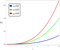
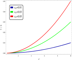
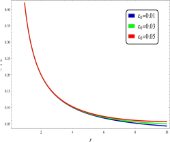
Figure 1: Picture represents the behavior of shape functions properties against the radial coordinate $r$ for the BEC model with $c_{1}=0.9$, $r_{0}=0.2$, $\rho_{s}=0.9$, and $R=1.94$.

III.2 Pseudo isothermal (PI)

In addition to the BEC-DM model, there is an important class of dark matter models associated with modified gravity, such as Modified Newtonian Dynamics (MOND) [85]. In the MOND model, the dark matter density profile is described by the PI profile

$$\rho_{\text{PI}}=\frac{\rho_{s}}{1+\left(\frac{r}{r_{s}}\right)^{2}},$$ (41)

where $\rho_{s}$ is the central dark matter density and $r_{s}$ is the scale radius.

III.2.1 Finding solution

The solution of mass profile for the PI galactic halo can be obtained using Eq. (27)

$$M(r)=4\pi\rho_{s}r_{s}^{2}\left(r-r_{s}\tan^{-1}\left(\frac{r}{r_{s}}\right)\right).$$ (42)

The tangential velocity $v_{t}^{2}(r)$ of a test particle moving in the dark halo is given by from Eq. (29)

$$v_{t}^{2}(r)=\frac{4\pi\rho_{s}r_{s}^{2}}{r}\left(r-r_{s}\tan^{-1}\left(\frac{r}{r_{s}}\right)\right).$$ (43)

Now, with the relation given in Eq. (31), we can find the redshift function

$$\phi(r)=2\pi\rho_{s}r_{s}^{2}\log\left(r^{2}+r_{s}^{2}\right)+\frac{4\pi\rho_{s}r_{s}^{3}\tan^{-1}\left(\frac{r}{r_{s}}\right)}{r}+D_{2},$$ (44)

where $D_{2}$ is the integrating constant. Now, we shall try to calculate the shape function of the wormhole under the PI dark matter model by comparing the density of the wormhole with the density of PI dark matter. From Eqs. (21) and (41), one can get the relation

$$\frac{c_{0}}{2}-\frac{c_{1}b^{\prime}(r)}{r^{2}}=\frac{\rho_{s}}{1+\left(\frac{r}{r_{s}}\right)^{2}}.$$ (45)

On solving

$$b(r)=\frac{\frac{c_{0}r^{3}}{3}+2\rho_{s}r_{s}^{3}\tan^{-1}\left(\frac{r}{r_{s}}\right)-2\rho_{s}rr_{s}^{2}}{2c_{1}}+c_{5},$$ (46)

where $c_{5}$ is the integrating constant. By imposing the throat condition on the above equation, we can obtain the final shape function

$$b(r)=\frac{1}{6c_{1}}\left[c_{0}r^{3}+6\rho_{s}r_{s}^{3}\Lambda_{4}+6\rho_{s}r_{s}^{2}(r_{0}-r)\right.\\ \left.-c_{0}r_{0}^{3}+6c_{1}r_{0}\right].$$ (47)

where

$$\Lambda_{4}=\left(\tan^{-1}\left(\frac{r}{r_{s}}\right)-\tan^{-1}\left(\frac{r_{0}}{r_{s}}\right)\right).$$ (48)

Now, we check the flare-out condition at the throat, i.e.,

$$b^{\prime}(r_{0})=\frac{\text{r1}^{2}r_{0}^{2}(c_{0}-2\rho_{s})+c_{0}r_{0}^{4}}{2c_{1}\left(r_{s}^{2}+r_{0}^{2}\right)},$$ (49)

which is obviously satisfied. For more information, one can check Fig 2.

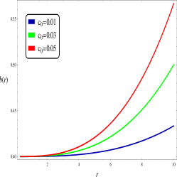
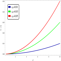
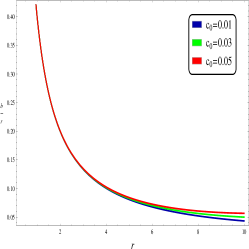
Figure 2: Picture represents the behavior of shape functions properties against the radial coordinate $r$ for the PI model with $c_{1}=0.9$, $r_{0}=0.2$, $\rho_{s}=0.9$, and $r_{s}=1.94$.

III.3 Navarro-Frenk-White (NFW)

An approximate analytical formulation of the NFW density profile is established by drawing upon the Cold Dark Matter ($\Lambda$CDM) theory and numerical simulations [86, 87]. In the context of galaxies and clusters, the dark matter halo can be characterized through the NFW density profile, expressed as

$$\rho(r)=\frac{\rho_{s}}{(r/r_{s})(1+r/r_{s})^{2}},$$ (50)

where $\rho_{s}$ denotes the dark matter density during the collapse of the dark matter halo, and $r_{s}$ represents the scale radius. It is widely recognized that the NFW density profile encompasses a diverse range of dark matter models characterized by minimal collision effects between dark matter particles.

III.3.1 Finding solution

For this case, the mass function can be read as

$$M(r)=4\pi\rho_{s}r_{s}^{3}\left(\frac{r_{s}}{r+r_{s}}+\log(r+r_{s})-\log(r_{s})-1\right),$$ (51)

and consequently, the tangential velocity $v_{t}^{2}(r)$ is

$$v_{t}^{2}(r)=\frac{4\pi\rho_{s}r_{s}^{3}}{r}\left(\frac{r_{s}}{r+r_{s}}+\log(r+r_{s})-\log(r_{s})-1\right).$$ (52)

Now from Eq. (31), we can find the redshift function

$$\phi(r)=\frac{4\pi\rho_{s}r_{s}^{3}}{r}\left(\log(r_{s})-\log(r+r_{s})\right)+D_{3},$$ (53)

where $D_{3}$ is the integrating constant. Again, from Eqs. (21) and (50), it follows that

$$\frac{c_{0}}{2}-\frac{c_{1}b^{\prime}(r)}{r^{2}}=\frac{\rho_{s}}{(r/r_{s})(1+r/r_{s})^{2}}$$ (54)

On solving the above differential equation, we obtain

$$b(r)=\frac{1}{2c_{1}}\left[-\frac{2\rho_{s}r_{s}^{4}}{r+r_{s}}-2\rho_{s}r_{s}^{3}\log(r+r_{s})+c_{0}r_{s}^{2}(r+r_{s})\right.\\ \left.-c_{0}r_{s}(r+r_{s})^{2}+\frac{1}{3}c_{0}(r+r_{s})^{3}\right]+c_{7},$$ (55)

where $c_{7}$ is the integrating constant. Now, we impose the condition $b(r_{0})=r_{0}$ on the above equation and obtain the shape function

$$b(r)=\frac{1}{6c_{1}}\left[c_{0}r^{3}+\Lambda_{6}+6\rho_{s}r_{s}^{3}\Lambda_{7}-c_{0}r_{0}^{3}+6c_{1}r_{0}\right],$$ (56)

where,

$$\Lambda_{6}=\frac{6\rho_{s}r_{s}^{4}(r-r_{0})}{(r+r_{s})(r_{s}+r_{0})},$$ (57)

$$\Lambda_{7}=(\log(r_{s}+r_{0})-\log(r+r_{s})).$$ (58)

Now, we study the important condition, i.e., flare-out condition, with the obtained shape function (56) graphically. We noticed that with the appropriate choices of parameters, the flare-out condition is satisfied, i.e., $b(r)<1$ at $r=r_{0}$ (see Fig. (3)).

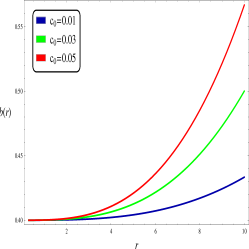
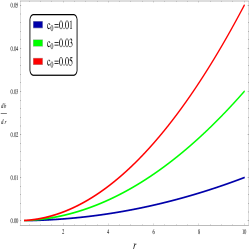
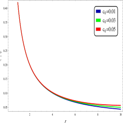
Figure 3: Picture represents the behavior of shape functions properties against the radial coordinate $r$ for the NFW model with $c_{1}=0.9$, $r_{0}=0.2$, $\rho_{s}=0.9$, and $r_{s}=1.94$.

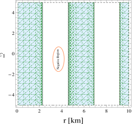
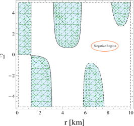
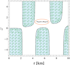
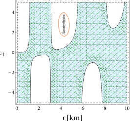
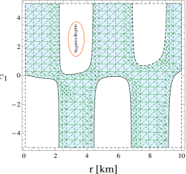
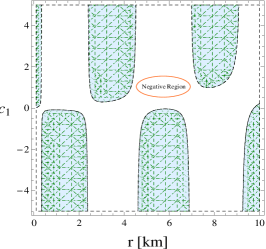
Figure 4: Picture represents the valid and negative regions of all the energy conditions for the BEC profile. In the first row $\rho$ (left), $\rho+p_{r}$ (middle), and $\rho+p_{t}$ (right) are presented. In second row, $\rho-p_{r}$ (left), $\rho-p_{t}$ (middle), and $\rho+p_{r}+2p_{t}$ (right) are shown with $c_{0}=0.05$, $r_{0}=0.2$, $\rho_{c}=0.9$, and $R=1.94$.

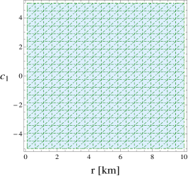
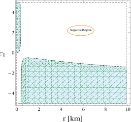
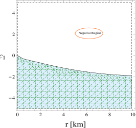
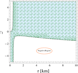
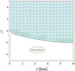
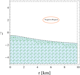
Figure 5: Picture represents the valid and negative regions of all the energy conditions for the PI profile. In the first row $\rho$ (left), $\rho+p_{r}$ (middle), and $\rho+p_{t}$ (right) are presented. In second row, $\rho-p_{r}$ (left), $\rho-p_{t}$ (middle), and $\rho+p_{r}+2p_{t}$ (right) are shown with $c_{0}=0.05$, $r_{0}=0.2$, $\rho_{s}=0.9$, and $r_{s}=1.94$.

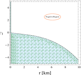
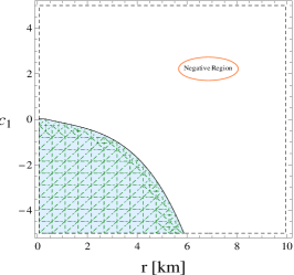
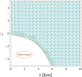
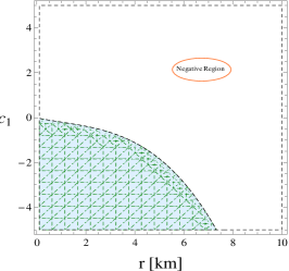
Figure 6: Picture represents the valid and negative regions of all the energy conditions for the NFW profile. In the first row $\rho$ (left), $\rho+p_{r}$ (middle), and $\rho+p_{t}$ (right) are presented. In second row, $\rho-p_{r}$ (left), $\rho-p_{t}$ (middle), and $\rho+p_{r}+2p_{t}$ (right) are shown with $c_{0}=0.05$, $r_{0}=0.2$, $\rho_{s}=0.9$, and $r_{s}=1.94$.

IV Energy conditions

In the study of modified gravitational theories, the validity of energy conditions of matter is often the key issue, and the ECs are the necessary conditions to explain the singularity theorem [88]. Moreover, the ECs aid in analyzing the entire space-time structure without precise solutions to Einstein’s equations and play a crucial role in investigating wormhole solutions in the context of modified gravity theories. The common popular basic energy conditions (the null, weak, dominant, and strong energy conditions) originate from the Raychaudhuri equation [89], which plays a crucial role in describing the attractive properties of gravity and positive energy density. The WEC [90] is defined by $T_{\mu\nu}U^{\mu}U^{\nu}\geq 0$ i.e.,

$$\rho\geq 0,\quad\rho+P_{r}\geq 0,\quad\rho+P_{t}\geq 0,$$ (59)

where $U^{\mu}$ denotes the time-like vector. This means that local energy density is positive, and it gives rise to the continuity of NEC, which is defined by $T_{\mu\nu}k^{\mu}k^{\nu}\geq 0$, i.e.,

$$\rho+P_{r}\geq 0,\quad\rho+P_{t}\geq 0,$$ (60)

where $k^{\mu}$ represents a null vector. On the other hand, strong energy condition (SEC) stipulates that

$$\rho+P_{r}\geq 0,\quad\rho+P_{t}\geq 0,\quad\text{and}\quad\rho+P_{r}+2P_{t}\geq 0$$ (61)

and the dominant energy conditions (DEC) are defined by

$$\rho\geq 0,\quad\rho-\mathinner{\!\left\lvert P_{r}\right\rvert}\geq 0,\quad\rho-\mathinner{\!\left\lvert P_{t}\right\rvert}\geq 0.$$ (62)

Now, with the above expressions, we check the behaviors of ECs.
The expression for radial NEC for the BEC DM profile can be read as

$$\rho+P_{r}=\frac{1}{6}\left[-3c_{0}+\frac{1}{r^{3}}\left(c_{0}r^{3}+\frac{1}{\pi^{3}}\left(6\rho_{s}R^{2}\right.\right.\right.\\ \left.\left.\left.\times\left(\pi\Lambda_{2}-R\Lambda_{1}\right)\right)-c_{0}r_{0}^{3}+6c_{1}r_{0}\right)-\frac{1}{\pi^{5}r^{4}}\left(8\rho_{s}R^{2}\right.\right.\\ \left.\left.\times\Lambda_{3}\left(\pi^{3}\left(-c_{0}r^{3}+6c_{1}r+c_{0}r_{0}^{3}-6c_{1}r_{0}\right)+6\rho_{s}R^{2}\right.\right.\right.\\ \left.\left.\left.\times\left(R\Lambda_{1}-\pi\Lambda_{2}\right)\right)\right)\right]+\frac{\rho_{s}R\sin\left(\frac{\pi r}{R}\right)}{\pi r},$$ (63)

where $\Lambda_{3}=\left(R\sin\left(\frac{\pi r}{R}\right)-\pi r\cos\left(\frac{\pi r}{R}\right)\right)$. $\Lambda_{1}$ and $\Lambda_{2}$ are defined in (38) and (39).
Similarly, for the PI case, NEC can be obtained as follows:

$$\rho+P_{r}=\frac{\rho_{s}r_{s}^{2}}{r^{2}+r_{s}^{2}}+\frac{1}{6r^{4}}\left[-3c_{0}r^{4}+r\left(c_{0}r^{3}+6\rho_{s}r_{s}^{3}\Lambda_{4}\right.\right.\\ \left.\left.+6\rho_{s}r_{s}^{2}(r_{0}-r)-c_{0}r_{0}^{3}+6c_{1}r_{0}\right)-8\pi\rho_{s}r_{s}^{2}\Lambda_{5}\left(-c_{0}r^{3}+6c_{1}r\right.\right.\\ \left.\left.-6\rho_{s}r_{s}^{3}\Lambda_{4}+6\rho_{s}r_{s}^{2}(r-r_{0})+c_{0}r_{0}^{3}-6c_{1}r_{0}\right)\right],$$ (64)

where, $\Lambda_{4}$ is already defined in (48) and $\Lambda_{5}=\left(r-r_{s}\tan^{-1}\left(\frac{r}{r_{s}}\right)\right)$.
At last, the expression for NEC for the NFW profile

$$\rho+P_{r}=-\frac{c_{0}}{2}+\frac{\Lambda_{6}+c_{0}r^{3}+6\Lambda_{7}\rho_{s}r_{s}^{3}-c_{0}r_{0}^{3}+6c_{1}r_{0}}{6r^{3}}\\ -\frac{1}{r^{4}(r+r_{s})}\left[8\pi c_{1}\rho_{s}r_{s}^{3}((r+r_{s})\Lambda_{8}+r)\left(\frac{1}{6c_{1}}\left(\Lambda_{6}+c_{0}r^{3}\right.\right.\right.\\ \left.\left.\left.+6\Lambda_{7}\rho_{s}r_{s}^{3}-c_{0}r_{0}^{3}+6c_{1}r_{0}\right)-r\right)\right]+\frac{\rho_{s}r_{s}^{3}}{r(r+r_{s})^{2}},$$ (65)

where $\Lambda_{8}=(\log(r_{s})-\log(r+r_{s}))$. The expression of $\Lambda_{6}$ and $\Lambda_{7}$ are presented in (57) and (58), respectively.
Now, at the throat ($r=r_{0}$), the NEC for each DM halo profile has been obtained and shown in Eq. (66).

$$\rho+P_{r}\bigg{|}_{r=r_{0}}=\begin{cases}-\frac{c_{0}}{2}+\frac{\rho_{s}R\sin\left(\frac{\pi r_{0}}{R}\right)}{\pi r_{0}}+\frac{c_{1}}{r_{0}^{2}},&\text{(BEC)}\\ \\ -\frac{c_{0}}{2}+\frac{\rho_{s}r_{s}^{2}}{r_{s}^{2}+r_{0}^{2}}+\frac{c_{1}}{r_{0}^{2}},&\text{(PI)}\\ \\ \frac{1}{r_{0}^{2}}\left[c_{1}+\frac{\rho_{s}r_{s}^{3}r_{0}}{(r_{s}+r_{0})^{2}}\right]-\frac{c_{0}}{2},&\text{(NFW)}\end{cases}$$ (66)

IV.1 Detailed analysis of these DM models with graphical descriptions

The primary focus of research has been on a method where the energy conditions are not violated by the actual matter itself but rather by an effective energy-momentum tensor that emerges within a modified gravitational theory framework. In this section, we will examine the energy conditions for the solutions we have explored. A comprehensive graphical analysis, including a regional investigation of the energy conditions in these dark matter models, is presented in Figs. (4-6). The energy density $\rho$ for the BEC model shows positive behavior in the vicinity of the throat within $-5\leq c_{1}\leq 5$ and $0\leq r\leq 2$. Interestingly, for the PI and NFW cases, energy density shows positive behavior in the entire space-time. Next, we plotted the radial NEC $\rho+P_{r}$ graphs for each case. It was noticed that for the BEC case, $\rho+P_{r}$ is violated near the throat for $-5\leq c_{1}\leq 0$ and $0\leq r\leq 1.7$, and satisfied for $0\leq c_{1}\leq 5$. For the PI case, the valid region of $\rho+P_{r}$ is $-5\leq c_{1}<-0.5$ and negative region is $-0.5\leq c_{1}<5$ against the radial co-ordinate $0.4\leq r\leq 10$. The energy condition $\rho+P_{r}$ for the NFW profile depicted violated for $0\leq c_{1}\leq 5$ and obeyed for $-5\leq c_{1}\leq 0$ within $0\leq r\leq 10$. Further, $\rho+P_{t}$ is depicted for each case and observed that it is disrespected for the BEC case within $0\leq c_{1}\leq 5$ and satisfied within $-5\leq c_{1}\leq 0$ against $0\leq r\leq 2.2$. Also, for the PI case, $\rho+P_{t}$ shows negative behavior for $c_{1}\geq 0$ whereas satisfied within $c_{1}<0$. In addition, $\rho+P_{t}$ for the NFW case portrays a valid region for $-5\leq c_{1}\leq 0$ and $0\leq r\leq 6$, and the remaining region shows the violation of $\rho+P_{t}$. Furthermore, we have thoroughly investigated the behavior of SEC, which can be found in the lower left plot of figures (4-6). We observed that the negative region of $\rho+P_{r}+2P_{t}$ for the BEC case is $0\leq c_{1}\leq 5$, PI case is $c_{1}>-0.5$, and for the NFW case is $c_{1}\geq 0$. Finally, we checked the behavior of DEC for each profile, and interestingly, we noticed that DEC’s behavior was completely opposite to NEC’s behavior. One can check figs. (4-6) for a complete overview. It is important to note that the model parameter, $c_{1}$, significantly influences all the energy conditions in the current analysis. In fact, within the range of parameters involved, all the energy conditions are violated in maximum regions, confirming the presence of exotic matter, which is necessary for creating the obtained wormhole solutions due to the violation of energy conditions, specifically the violation of NEC. This exotic matter is believed to contribute to the stability and traversability of wormholes by counteracting the gravitational collapse caused by ordinary matter. The study of energy violation in the context of wormholes sheds light on these structures. The energy conditions for each case (as shown in Figs. (4-6)) support the existence of these wormhole solutions in the background of symmetric teleparallel gravity.
All the results mentioned above regarding the energy conditions for each DM model are also summarized in Table-1

The behavior of the energy conditions around the throat
Physical expressions	BEC profile
$\rho$	$\rho>0$ for $-5\leq c_{1}\leq 5$
$\rho+p_{r}$	$\rho+p_{r}<0$ for $-5\leq c_{1}\leq 0$ and $\rho+p_{r}>0$ for $0\leq c_{1}\leq 5$
$\rho+p_{t}$	$\rho+p_{t}<0$ for $0\leq c_{1}\leq 5$ and $\rho+p_{t}>0$ for $-5\leq c_{1}\leq 0$
$\rho+p_{r}+2p_{t}$	$\rho+p_{r}+2p_{t}<0$ for $0\leq c_{1}\leq 5$ and $\rho+p_{r}+2p_{t}>0$ for $-5\leq c_{1}\leq 0$
$\rho-\mathinner{\!\left\lvert p_{r}\right\rvert}$	$\rho-\mathinner{\!\left\lvert p_{r}\right\rvert}<0$ for $0\leq c_{1}\leq 5$ and $\rho-\mathinner{\!\left\lvert p_{r}\right\rvert}>0$ for $-5\leq c_{1}\leq 0$
$\rho-\mathinner{\!\left\lvert p_{t}\right\rvert}$	$\rho-\mathinner{\!\left\lvert p_{t}\right\rvert}<0$ for $-5\leq c_{1}\leq 0$ and $\rho-\mathinner{\!\left\lvert p_{t}\right\rvert}>0$ for $0\leq c_{1}\leq 5$
PI profile
$\rho$	$\rho>0$ for $-5\leq c_{1}\leq 5$
$\rho+p_{r}$	$\rho+p_{r}<0$ for $-0.5\leq c_{1}<5$ and $\rho+p_{r}>0$ for $-5\leq c_{1}<-0.5$
$\rho+p_{t}$	$\rho+p_{t}<0$ for $c_{1}\geq 0$ and $\rho+p_{t}>0$ for $c_{1}<0$
$\rho+p_{r}+2p_{t}$	$\rho+p_{r}+2p_{t}<0$ for $c_{1}>-0.5$ and $\rho+p_{r}+2p_{t}>0$ for $c_{1}\leq-0.5$
$\rho-\mathinner{\!\left\lvert p_{r}\right\rvert}$	$\rho-\mathinner{\!\left\lvert p_{r}\right\rvert}<0$ for $-5\leq c_{1}<-0.5$ and $\rho-\mathinner{\!\left\lvert p_{r}\right\rvert}>0$ for $-0.5\leq c_{1}<5$
$\rho-\mathinner{\!\left\lvert p_{t}\right\rvert}$	$\rho-\mathinner{\!\left\lvert p_{t}\right\rvert}<0$ for $c_{1}<0$ and $\rho-\mathinner{\!\left\lvert p_{t}\right\rvert}>0$ for $c_{1}\geq 0$
NFW profile
$\rho$	$\rho>0$ for $-5\leq c_{1}\leq 5$
$\rho+p_{r}$	$\rho+p_{r}<0$ for $0\leq c_{1}<5$ and $\rho+p_{r}>0$ for $-5\leq c_{1}<0$
$\rho+p_{t}$	$\rho+p_{t}<0$ for $c_{1}\geq 0$ and $\rho+p_{t}>0$ for $-5\leq c_{1}<0$
$\rho+p_{r}+2p_{t}$	$\rho+p_{r}+2p_{t}<0$ for $c_{1}\geq 0$ and $\rho+p_{r}+2p_{t}>0$ for $0<c_{1}\leq-5$
$\rho-\mathinner{\!\left\lvert p_{r}\right\rvert}$	$\rho-\mathinner{\!\left\lvert p_{r}\right\rvert}<0$ for $-5\leq c_{1}<0$ and $\rho-\mathinner{\!\left\lvert p_{r}\right\rvert}>0$ for $0\leq c_{1}\geq 5$
$\rho-\mathinner{\!\left\lvert p_{t}\right\rvert}$	$\rho-\mathinner{\!\left\lvert p_{t}\right\rvert}<0$ for $-5\leq c_{1}<0$ and $\rho-\mathinner{\!\left\lvert p_{t}\right\rvert}>0$ for $c_{1}\geq 0$

Table 1: Outlook of the energy conditions

V Shadows of Wormholes

In this section, we shall discuss wormhole shadows under the effect of three different kinds of dark matter halos, including BEC. To study the impact of wormholes on light deflection, we need to calculate the movement of light rays. We consider the motion of a light beam using the null geodesic equation, which allows us to predict its trajectory. The equation can be found by applying the Euler-Lagrange equation: $\mathcal{L}=-\frac{1}{2}g_{\mu\nu}\dot{x}^{\mu}\dot{x}^{\nu}$. Without loss of generality, we can consider the equatorial plane, i.e., $\theta=\frac{\pi}{2}$. The Lagrangian equation describing the motion of light rays around the wormhole geometry is given as

$$\begin{split}&\mathcal{L}=-\frac{1}{2}g_{\mu\nu}\dot{x}^{\mu}\dot{x}^{\nu}\\ &=-e^{2\phi(r)}\dot{t}^{2}+\frac{1}{1-\frac{b(r)}{r}}\dot{r}^{2}+r^{2}(\dot{\theta}^{2}+\sin^{2}\theta\dot{\Phi}^{2}),\\ \end{split}$$ (67)

where $\dot{x}^{\mu}$ denotes the four-velocity of the photon, and the dot represents the differentiation with respect to the affine parameter $\tau$. Now, by applying the Lagrangian equation of motion within the scope of wormhole geometry in Eq. (67), one can get the following relations

$$\dot{t}=\frac{dt}{d\tau}=\frac{E}{e^{2\phi(r)}},$$ (68)

$$\dot{\Phi}=\frac{d\Phi}{d\tau}=\frac{L}{r^{2}\sin^{2}(\theta)}.$$ (69)

In the above relations, $E$ and $L$ represent the energy and angular momentum of the particle around the wormhole throat. To simplify the geodesics, we propose two dimensionless impact parameters: $\xi=\frac{L}{E}$ and $\eta=\frac{\kappa}{E^{2}}$, where $\kappa$ denotes the Carter constant. By considering the null geodesic ($\mathcal{L}=0$), which can be expressed in terms of kinetic and potential energy. Scale an affine parameter $\tau\rightarrow\frac{\tau}{L}$. The orbit equation of motion can be revised as:

$$K_{E}+V_{eff}=\frac{1}{\tilde{b}^{2}},$$ (70)

where $\tilde{b}=\frac{L}{E}$ is the kinetic energy function $K_{E}$ and potential function $V_{eff}$ are described as

$$K_{E}=\frac{e^{2\phi(r)}}{1-\frac{b(r)}{r}}\dot{r}^{2},$$ (71)

and

$$V_{eff}=\frac{e^{2\phi(r)}}{r^{2}}.$$ (72)

In order to describe the wormhole shadows around the wormhole throat, one can use celestial coordinates ($X,Y$), which are further defined as:

$$X=\lim_{r_{0}\rightarrow\infty}(-r_{0}^{2}\sin(\theta_{0}))\frac{d\phi}{dr},\quad Y=\lim_{r_{0}\rightarrow\infty}(r_{0}^{2}\frac{d\theta}{dr}),$$ (73)

where $r_{0}$ is the wormhole throat. Further, $\theta_{0}$ is the inclination angle between the wormhole and the observer. After some simplification, one can obtain the celestial coordinates for wormhole geometry as

$$X=-\frac{\xi}{\sin(\theta_{0})},\quad Y=\sqrt{\eta-\frac{\xi^{2}}{\tan^{2}(\theta_{0})}}.$$ (74)

Assuming the static observer is at infinity, the radius of the wormhole shadow $R_{s}$ as seen from the equatorial plane, i.e., $\theta_{0}=\pi/2$ can be stated as:

$$R_{s}=\sqrt{\xi^{2}+\eta}=\frac{r_{0}}{e^{\phi(r_{0})}}.$$ (75)

The parametric plot for the equations (74) and (75) in the $(X,Y)$ plane can cast a variety of wormhole shadows for the different ranges of involved parameters. The wormhole shadows for the wormhole geometry are depicted in Fig.(7) for three models of dark matter halos, including BEC. From the first row of Fig.(7), it is noticed that the BEC profile has an influence on the wormhole shadows. The larger values of $D_{1}$ and central density $\rho_{c}$ lead the wormhole shadow closer to the wormhole throat. For the smaller values of these mentioned parameters wormhole shadow radius is going away from the wormhole throat. The same behavior is also noticed for two other cases, the PI profile and NFW profile from the second row and third row of Fig.(7).

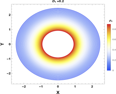
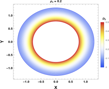
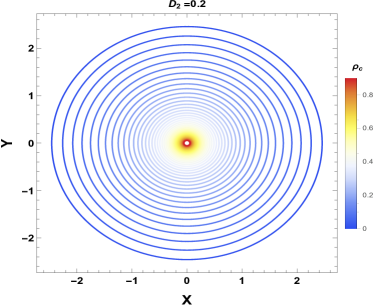
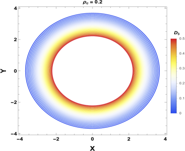
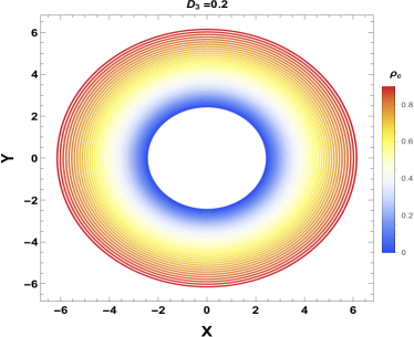
Figure 7: Picture represents the parametric plots for wormhole shadows with BEC profile (first row), PI profile (second row), and NFW profile (third row) with $r_{0}=0.2$, $R=1.94$, and $r_{s}=1.94$.

VI Deflection angle

This section deals with the deflection angle cast by wormhole geometry under the effect of three different kinds of dark matter halos. The mass and energy generate the curvature of space-time, which influences the speed of light. The curvature of space-time can cause light to bend near a big object, such as a black hole or wormhole. The fascination among researchers with gravitational lensing, especially its strong form, has seen a notable increase following the works by Virbhadra and colleagues [92, 93, 94]. Additionally, Bozza, in Ref. [70], introduced an analytical approach to compute gravitational lensing in the strong field limit for any spherical symmetric space-time. This method has been applied in numerous subsequent studies, such as Refs. [95, 96]. This background encourages us to use this analytical technique in our current research. We adopt a numerical technique to study the deflection angle near the wormhole’s throat to achieve this aim. The formula for deflection angle $\alpha$ for the Morris-Thorne Wormhole geometry can be read as [91]

$$\alpha=-\pi+2\int_{r_{c}}^{\infty}\frac{e^{\phi(r)}dr}{r^{2}\sqrt{(1-\frac{b(r)}{r})(\frac{1}{\beta^{2}}-\frac{e^{2\phi(r)}}{r^{2}})}},$$ (76)

where $r_{s}$ is the closest path of light near the throat and $\beta$ is the impact parameter. For null geodesic, we have the relation between $\beta$ and $r_{s}$, defined by

$$\beta=r_{c}e^{-\phi(r_{c})}.$$ (77)

We obtained redshift and shape functions in the previous sections for three dark matter models. Here, we shall use those redshift and shape functions to study the deflection angles around the throat. We substitute the three different sets of redshift functions by Eq. (33), Eq. (44), and Eq. (53) and shape functions by Eq. (35), Eq. (46), and Eq. (55) into Eq.(76) and solve numerically, one can get deflection angle $\alpha$ with respect to $r_{c}$ for three different backgrounds. Fig. 8 shows that the deflection angle tends to zero as the distance $r_{c}$ increases to infinity. In other words, as the light ray goes away from the wormhole throat, where the gravitational field of the wormhole is negligible, it does not deflect from the original path. When the value of the distance $r_{c}$ is close to the radius of the wormhole throat, the deflection angle increases significantly. In the wormhole throat, where the gravitational field is extremely strong, the deflection of light tends to infinity.

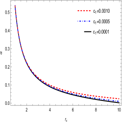
Figure 8: Picture represents the deflection angle for BEC (left), PI (middle), and NFW (right) profiles with $c_{0}=0.05$, $R=1.94$, $r_{0}=0.2$, $\rho_{s}=0.9$, and $r_{s}=1.94$.

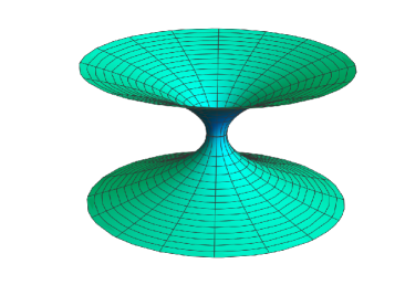
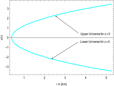
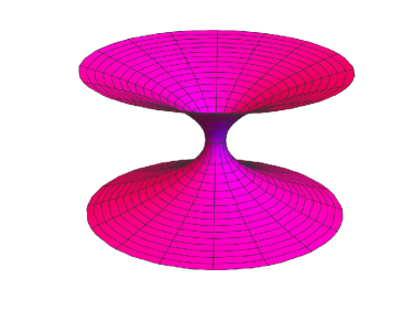
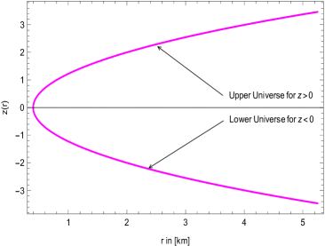
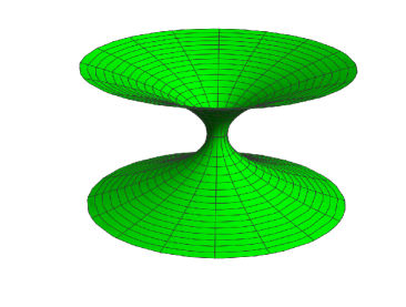
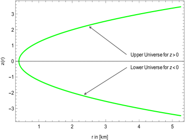
Figure 9: Picture represents the connection of upper and lower Universes through the embedding surface with $c_{0}=0.05$, $R=1.94$, $r_{0}=0.2$, $\rho_{s}=0.9$, and $r_{s}=1.94$.

VII Embedding diagram

In this segment, we shall delve into the use of embedding diagrams to gain insights into the structure of wormhole space-time, as referenced in Eq. (1). Our focus is squarely on geometry, which leads us to impose certain constraints on the choice of coordinates. We set $\theta=\pi/2$ on the equatorial plane and fixing time ($t=$ constant). Under these conditions, Eq. (1) simplifies to

$$ds^{2}=\left(1-\frac{b(r)}{r}\right)^{-1}+r^{2}d\phi^{2}.$$ (78)

We then adapt this modified metric to fit within a three-dimensional Euclidean framework, employing cylindrical coordinates $(r,\,\phi,\,z)$, which yields

$$ds^{2}=dz^{2}+dr^{2}+r^{2}d\phi^{2}.$$ (79)

By comparing the two equations above, we deduce the shape of the embedding surface $z(r)$, leading us to establish a gradient as follows:

$$\frac{dz}{dr}=\pm\sqrt{\frac{r}{r-b(r)}-1}.$$ (80)

Eq. (80) shows that the embedded surface becomes vertical at the throat, i.e., $\frac{dz}{dr}$ approaches infinity. Furthermore, it is observed that as r increases towards infinity, indicating the distance from the throat, the curvature, represented by $\frac{dz}{dr}$, tends towards zero, suggesting the space becomes flat. Now, substituting the shape functions given in Eqs. (35), (46), and (55) into the Eq. (80), we have plotted the embedding diagram, which can be found in Fig. 9. In these figures, a positive curvature, $z>0$, denotes the upper universe, while a negative curvature, $z<0$, represents the lower universe.

VIII Conclusions

In this study, we have uncovered a novel wormhole solution sustained by DM frameworks such as BEC, PI, and NFW within the $f(Q)$ gravity theory framework. Specifically, our approach involved utilizing the density profile equations of the DM frameworks in conjunction with the rotational velocity to determine both the redshift and shape functions of the wormholes. It is critical to highlight that the model’s parameters significantly impact the investigation of the shape of the wormhole. Our findings demonstrate that choosing particular parameters, including the wormhole throat radius $r_{0}$, leads to a wormhole solution that meets the flare-out condition at the throat, maintaining this characteristic under an asymptotic background. Further, we have investigated the energy conditions using the same parameter involved in the shape functions. Mathematically, we have calculated the expressions of NEC for each model at the throat (see Eq. (66)). Also, we have depicted the positive and negative regions of all the energy conditions in Figs. (4-6) as well as summarized in Table- 1.
Furthermore, we have investigated the wormhole shadow under the effect of DM models. Our findings indicate that the BEC DM model influences the wormhole shadow. Specifically, larger values of $D_{1}$ and central density $\rho_{s}$ bring the wormhole shadow closer to the throat, while smaller values of these parameters push the shadow radius away from the throat. We have also observed similar behavior for the PI and NFW profiles.
In addition to the shadow, we have studied the gravitational lensing cast by wormhole geometry under three DM models in the context of $f(Q)$ gravity. Our results show that as the distance $r_{c}$ increases towards infinity, the deflection angle tends to zero, meaning that the light ray will not deviate from its original path as it moves away from the wormhole throat, where the gravitational field is weak. However, as the distance $r_{c}$ approaches the radius of the wormhole throat, the deflection angle increases significantly. At the throat, where the gravitational field is extremely strong, the deflection of light tends toward infinity.
Thus, it is safe to conclude that our findings suggest the possibility of the existence of wormholes in the galactic halos caused by BEC, PI, and NFW dark matter within the framework of $f(Q)$ gravity. Additionally, the effect of these dark matter models could be explored in other modified gravity theories, such as $f(T)$ gravity, as both $f(T)$ and $f(Q)$ models are indistinguishable at the cosmological background level [97].

Data Availability

There are no new data associated with this article.

- [1] B. P. Abbott et al., LIGO Scientific Collaboration, Virgo Collaboration, Phys. Rev. Lett. 116, 061102 (2016).
- [2] B. P. Abbott et al., LIGO Scientific Collaboration, Virgo Collaboration, Phys. Rev. Lett. 121, 129902 (2018).
- [3] K. Akiyama et al., Event horizon telescope, Astrophys. J. 875, L1 (2019).
- [4] A. Einstein and N. Rosen, Phys. Rev. 48, (1935) 73.
- [5] H. G. Elis, J. Math. Phys. (N.Y.) 14, 104 (1973).
- [6] M. S. Morris and K. S. Thorne, Am. J. Phys. 56, 395-412 (1988).
- [7] V. Khatsymovsky, Phys. Lett. B 320, 234 (1994).
- [8] H. A. Shinkai and S. A. Hayward, Phys. Rev. D 66, 044005 (2002).
- [9] D. Roy, A. Dutta, and S. Chakraborty, Europhys. Lett. 140, 19002 (2022).
- [10] H. Fukutaka, K. Tanaka, and K. Ghoroku, Phys. Lett. B 222, 191 (1989).
- [11] D. Hochberg, Phys. Lett. B 251, 349 (1990).
- [12] K. Ghoroku and T. Soma, Phys. Rev. D 46, 1507 (1992).
- [13] N. Furey and A. DeBenedictis, Class. Quant. Grav. 22, 313 (2005).
- [14] K .A. Bronnikov and E. Elizalde, Phys. Rev. D 81, 044032 (2010).
- [15] P. Kanti, B. Kleihaus and J. Kunz, Phys. Rev. Lett. 107, 271101 (2011).
- [16] T. Harko, F. S. N. Lobo, M. K. Mak and S. V. Sushkov, Phys. Rev. D 87, 067504 (2013).
- [17] R. Sengupta, S. Ghosh, M. Kalam, and S. Ray, Class. Quant. Grav. 39, 105004 (2022).
- [18] J. B. Jimenez, L. Heisenberg, T. Koivisto, Phys. Rev. D, 98, 044048 (2018).
- [19] Rui-Hui Lin and Xiang-Hua Zhai, Phys. Rev. D 103, 124001 (2021).
- [20] J. B. Jimenez, L. Heisenberg, T. Koivisto, and S. Pekar, Phys. Rev. D 101, 103507 (2020).
- [21] B. J. Barros et al., Phys. Dark Univ. 30, 100616 (2020).
- [22] N. Frusciante, Phys. Rev. D 103, 044021 (2021).
- [23] T. Harko, T. S. Koivisto, F. S. N. Lobo, G. J. Olmo, and D. Rubiera-Garcia, Phys. Rev. D 98, 084043 (2018).
- [24] F. K. Anagnostopoulos, V. Gakis, E. N. Saridakis, and S. Basilakos, Eur. Phys. J. C 83, 58 (2023).
- [25] R. Lazkoz, F. S. N. Lobo, M. OrtizBanos, and V. Salzano, Phys. Rev. D 100, 104027 (2019).
- [26] K. Flathmann and M. Hohmann, Phys. Rev. D 103, 044030 (2021).
- [27] W. Khyllep, J. Dutta, E. N. Saridakis, and K. Yesmakhanova, Phys. Rev. D 107, 044022 (2023).
- [28] G. N. Gadbail, A. Kolhatkar, S. Mandal, and P. K. Sahoo Eur. Phys. J. C 83 595, (2023).
- [29] D. S. Rana, R. Solanki, and P.K. Sahoo, Phys. Dark Univ. 43, 101421 (2024).
- [30] F. D’Ambrosio, Shaun D. B. Fell, L. Heisenberg, and S. Kuhn Phys. Rev. D 105, 024042 (2022).
- [31] Jose Tarciso S. S. Junior and Manuel E. Rodrigues Eur. Phys. J. C 83, 475 (2023).
- [32] Dhruba Jyoti Gogoi, Ali Ovgun, and M. Koussour Eur. Phys. J. C 83, 700 (2023).
- [33] S. K. Maurya et al. Eur. Phys. J. C 83, 317 (2023).
- [34] O. Sokoliuk, Sneha Pradhan, P. K. Sahoo, and Alexander Baransky Eur. Phys. J. Plus 137, 1077 (2022).
- [35] Wenyi Wang, Hua Chen, and Taishi Katsuragawa, Phys. Rev. D 105, 024060 (2022).
- [36] Marco Calza and Lorenzo Sebastiani, Eur. Phys. J. C 83, 247 (2023).
- [37] G. Mustafa et al., Phys. Lett. B 821, 136612 (2021).
- [38] Z. Hassan, S. Mandal, and P. K. Sahoo, Fortschr. Phys. 69, 2100023 (2021).
- [39] U. K. Sharma, Shweta, and A. K. Mishra, Int. J of Geo. Methods Mod. Phys. 02, 2250019 (2022).
- [40] Z. Hassan, S. Ghosh, P. K. Sahoo, and K. Bamba, Eur. Phys. J. C 82, 1116, (2022).
- [41] Z. Hassan, S. Ghosh, P. K. Sahoo, and V. S. Hari Rao, Gen. Relativ. Gravit. 55, 90 (2023).
- [42] A. Banerjee, A. Pradhan, T. Tangphati, and F. Rahaman, Eur. Phys. J. C 81, 1031 (2021).
- [43] F. Parsaei, S. Rastgoo, and P. K. Sahoo Eur. Phys. J. Plus 137, 1083 (2022).
- [44] J. Lu, S. Yang, Y. Liu, Y. Zhang, and Yu Liu, Eur. Phys. J. Plus 139, 274 (2024),
- [45] M. Tayde et al., Phys. Dark Univ. 42, 101288 (2023).
- [46] S. Kiroriwal et al., Fortschr. Phys., 2300197 (2024).
- [47] S. K. Maurya et al., Fortschr. Phys., 2300229 (2024).
- [48] V. C. Rubin, W. K. Jr. Ford, and N. Thonnard Astrophys. J. 238, 471-487 (1980).
- [49] F. Zwicky, Gen. Relativ. Gravit. 41, 207-224 (2009).
- [50] P. A. R. Ade et al., Astron. Astrophys. 594, A13 (2016).
- [51] F. Rahaman, P. K. F. Kuhfittig, S. Ray and N. Islam Eur. Phys. J. C 74, 2750 (2014).
- [52] F. Rahaman, P. Salucci, K. F. Kuhfittig, S. Ray and M. Rahaman Ann. Phys., 350, 561 (2014).
- [53] J. F. Navarro, C. S. Frenk and S. D. M. White Astrophys. J. 462, 563 (1996).
- [54] F. Rahaman, G. C. Shit, B. Sen and S. Ray, Astrophys. Space Sci. 361 37 (2016).
- [55] S. Islam, F. Rahaman, A. Ovgun and M. Halilsoy Can. J. Phys. 97, 241 (2019).
- [56] P. Salucci and Ch. Frigerio Martins, EAS Publ. Ser. 36, 133 (2009).
- [57] K. Jusufi, M. Jamil and M. Rizwan, Gen. Relativ. Gravit. 51, 102 (2019).
- [58] J. Einasto, and U. Haud, Galaxy Astron. Astrophys. 223 89 (1989).
- [59] K. G. Begeman, A. H. Broeils and R. H. Sanders, Mon. Not. R. Astron. Soc. 249, 523 (1991).
- [60] M. Milgrom, Phys. Rev. Lett. 117, 141101 (2016).
- [61] M. Milgrom, Astrophys. J. 270, 365 (1983).
- [62] M. Milgrom, Astrophys. J. 270 371 (1983).
- [63] B. C. Paul, Class. Quantum Grav. 38, 145022 (2021).
- [64] A. Einstein, Science 84, 506 (1936).
- [65] F. W. Dyson, A. S. Eddington, and C. Davidson, Philos. Trans. R. Soc. A 220, 291 (1920).
- [66] A. S. Eddington, ”Space, Time and Gravitation,” Cambridge University Press, Cambridge, England, (1920).
- [67] K. C. Sahu et al., Science 356, 1046 (2017).
- [68] V. Bozza et al., Gen. Relativ. Gravit. 33, 1535 (2001).
- [69] K. S. Virbhadra, G.F.R. Ellis, Phys. Rev. D 62, 084003 (2000).
- [70] V. Bozza, Phys. Rev. D 66, 103001 (2002).
- [71] N. Tsukamoto, Phys. Rev. D 94, 124001 (2016).
- [72] Y. Kumaran and A. Ovgun, Turk. J. Phys. 45, 247-267 (2021).
- [73] A. Ovgun, Turk. J. Phys. 44, 465-471 (2020).
- [74] W. Javed, R. Babar, and A. Ovgun, Phys. Rev. D 99, 084012 (2019).
- [75] R. Shaikh and S. Kar, Phys. Rev. D 96, 044037 (2017).
- [76] A. Ovgun, Phys. Rev. D 98, 044033 (2018).
- [77] K. Jusufi and A. Ovgun, Phys. Rev. D 97, 024042 (2018).
- [78] W. Javed et al., Eur. Phys. J. C 82, 1057 (2022).
- [79] S. N. Sajadi and N. Riazi, Can. J. Phys. 98, 1046-1054 (2020).
- [80] W. Javed et al., Universe 8, 599 ( 2022).
- [81] J. B. Jimenez, L. Heisenberg, T. Koivisto, S. Pekar, Phys. Rev. D 101, 103507 (2020).
- [82] C. G. Boehmer, T. Harko, JCAP 0706, 025 (2007).
- [83] F. Dalfovo, S. Giorgini, L. P. Pitaevskii and S. Stringari, Rev. Mod. Phys. 71, 463 (1999).
- [84] T. Harko, P. Liang, S. D. Liang, and G. Mocanu, JCAP 1511, 027 (2015).
- [85] K. G. Begeman, A. H. Broeils, and R. H. Sanders, MNRAS 249, 523 (1991).
- [86] J. F. Navarro, C. S. Frenk, and S. D. M. White, Astro. J. 462, 563 (1996).
- [87] J. F. Navarro, C. S. Frenk, and S. D. M. White, Astro. J. 490, 493 (1997).
- [88] S. W. Hawking and G. F. R. Ellis, Cambridge University Press, England, (1973).
- [89] A. Raychaudhuri, Phys. Rev. 98, 1123 (1955).
- [90] M. Visser, Lorentzian Wormholes (New York: AIP Press), (1996).
- [91] V. Bozza, et al., Gen. Relat. Grav. 33, 1535 (2001).
- [92] K. S. Virbhadra, D. Narasimha, and S. M. Chitre, Astron. Astrophys. 337, 1 (1998).
- [93] K. S. Virbhadra and G. F. R. Ellis, Phys. Rev. D 62, 084003 (2000).
- [94] C. M. Claudel, K. S. Virbhadra, and G. F. R. Ellis, J. Math. Phys. 42, 818 (2001).
- [95] J. P. S. Lemos, F. S. N. Lobo, and S. Quinet de Oliveira, Phys. Rev. D 68, 064004 (2003).
- [96] J. M. Tejeiro and E. A. Larranaga, Rom. J. Phys. 57, 736 (2012).
- [97] J. B. Jimenez, L. Heisenberg, T. Koivisto, S. Pekar, Phys. Rev. D 101, 103507 (2020).