Simple-Sampling and Hard-Mixup with Prototypes to Rebalance Contrastive Learning for Text Classification

Abstract

Text classification is a crucial and fundamental task in natural language processing. Compared with the previous learning paradigm of pre-training and fine-tuning by cross entropy loss, the recently proposed supervised contrastive learning approach has received tremendous attention due to its powerful feature learning capability and robustness. Although several studies have incorporated this technique for text classification, some limitations remain. First, many text datasets are imbalanced, and the learning mechanism of supervised contrastive learning is sensitive to data imbalance, which may harm the model performance. Moreover, these models leverage separate classification branch with cross entropy and supervised contrastive learning branch without explicit mutual guidance. To this end, we propose a novel model named SharpReCL for imbalanced text classification tasks. First, we obtain the prototype vector of each class in the balanced classification branch to act as a representation of each class. Then, by further explicitly leveraging the prototype vectors, we construct a proper and sufficient target sample set with the same size for each class to perform the supervised contrastive learning procedure. The empirical results show the effectiveness of our model, which even outperforms popular large language models across several datasets.

1 Introduction

Text classification (TC), as one of the fundamental tasks in the field of natural language processing (NLP), has attracted much attention from academia and industry and is widely used in various fields, such as question answering Liu et al. (2023a, b) and topic labeling tasks Wang et al. (2016); Liu et al. (2021). In TC processes, the ability of the model to extract textual features from raw text is crucial to the model performance Liu et al. (2021, 2024b). Text data in the form of symbolic sequences are extremely different from image data, and their discrete nature makes feature extraction and information utilization time-consuming and inefficient. Early TC models rely mainly on manual feature engineering such as bag-of-words or n-grams, to represent texts. Such predefined features are typically highly sparse and show limited expressive power Li et al. (2020a). Later, with the development of deep models, deep learning techniques led to a revolution in machine learning, and models such as convolutional neural networks (CNNs) Kim (2014) and recurrent neural networks (RNNs) Liu et al. (2015) based on deep neural networks came into being. Based on that, large-scale pre-trained language models (PLMs) such as BERT Devlin et al. (2019) and RoBERTa Liu et al. (2019), emerged and have shown great superiority in text mining. In the era of large language models (LLMs), some popular ones such as GPT-3.5 Ouyang et al. (2022) and Llama Touvron et al. (2023) have also achieved impressive performance in general text understanding. However, they may not perform as well as desired in domain-specific (e.g, medical or legal domains) texts Chang et al. (2023).

Owing to the remarkable performance of large-scale pre-trained models, the learning paradigm of pre-training and fine-tuning has emerged as the new standard across various fields. In NLP classification tasks, numerous models adhere to this paradigm and are fine-tuned under the guidance of cross-entropy (CE) loss to adapt to downstream tasks Devlin et al. (2019); Liu et al. (2019). Despite achieving state-of-the-art results on many datasets, CE loss exhibits certain limitations: a number of studies Liu et al. (2019); Cao et al. (2019) have demonstrated that CE results in reduced generalization capabilities and lacks robustness to data noise Sukhbaatar et al. (2015). Furthermore, CE exhibits instability across different runs when employed for fine-tuning in NLP tasks, potentially impeding the model from attaining optimal performance Zhang and Sabuncu (2018); Dodge et al. (2020).

Recently, the emerging contrastive learning (CL) has showcased impressive representation learning capabilities and has been extensively applied in both computer vision and NLP domains Chen et al. (2020); He et al. (2020); Gao et al. (2021). Notably, supervised contrastive learning (SCL) Khosla et al. (2020), a supervised variant of CL, aims to incorporate label information to extend the unsupervised InfoNCE loss to a supervised contrastive loss. This approach brings the representations of samples belonging to the same class closer together while pushing those of different classes apart. Some work Hendrycks and Dietterich (2020) has demonstrated that SCL is less sensitive to hyperparameters in optimizers and data augmentation, exhibiting enhanced stability. Consequently, several studies Gunel et al. (2021); Chen et al. (2022) have attempted to merge the learning methods of SCL and cross-entropy loss for fine-tuning PLMs, achieving considerable success.

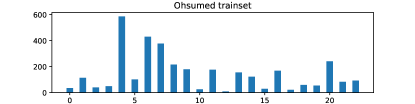
Figure 1: Label distribution of the Ohsumed trainset. The horizontal coordinate denotes the category, and the vertical coordinate denotes the corresponding frequency.

Despite the fruitful success of previous SCL-based models in TC tasks, there are several limitations that hinder the performance of these models. First, they all assume that the models are trained on large-scale, sufficient and balanced datasets, where each class has adequate and equal training samples Zhu et al. (2022). However, in real-world application scenarios, the label distribution of data is often imbalanced. Especially when there are many classes in the dataset, many of which (minority class) have few samples, and a handful (majority class) have numerous samples. As shown in Fig. 1, existing TC datasets such as the Ohsumed dataset Yao et al. (2019) are often class-imbalanced. When deep models are trained with such datasets, they may yield suboptimal results and even suffer from overfitting problems, especially in minority classes Zhang et al. (2021); Yang et al. (2022). Meanwhile, the manner of SCL in selecting positive and negative pairs also makes it more sensitive to data imbalance. Specifically, we suppose that the batch is $B$ and the imbalance ratio of the batch is $ir=\frac{\pi_{max}}{\pi_{min}}$, where $\pi_{max}$ and $\pi_{min}$ are the frequencies of the majority class and the minority class in the original dataset, respectively. Since each instance should select samples from the same class to form the positive pairs and from other classes to form the negative pairs, the imbalance ratio can be further written as $ir=\frac{({|B|\pi_{max}})^{2}}{({|B|\pi_{min}})^{2}}=(\frac{{\pi_{max}}}{{\pi_{min}}})^{2}$ (the detailed analysis is shown in the “Preliminaries” section). That means when performing SCL on imbalanced datasets, the imbalance ratio is quadratic, and the imbalanced issue becomes more severe. Moreover, when the class imbalance problem exists in the dataset, samples may not encounter the proper positive or negative samples within a batch in the SCL paradigm Song et al. (2022). That is, the majority class samples may lack sufficient negative samples and the minority class samples can also lack adequate positive samples. Therefore, obtaining excellent model performance when performing SCL for imbalanced TC tasks is a great challenge, and there has been little effort to explore it.

Second, previous models Gunel et al. (2021); Suresh and Ong (2021) commonly utilize labeled data in two different branches, i.e., learning separately by following the paradigm of CE and of SCL and then obtaining the final training loss by a weighted average of the corresponding losses. However, such approaches only superficially combine CE and SCL, without any component or architecture linking CE and SCL to make them carry out further display interactions. It is also worth noting that the labeled data utilized for CE and SCL are the same, and these two modules both aim to achieve the effect of aggregating samples from the same class while separating samples from different classes. Therefore, further extracting effective information from these two supervised learning modules in an interactive manner to guide model training remains a challenge.

To address the above issues, we propose SharpReCL, meaning Simple-Sampling and Hard-Mixup with Prototypes to Rebalance Contrastive Learning for TC. To address the problem of lack of mutual guidance between the two learning branches, we leverage the classification branch to compute class prototype vectors, which also appear in the SCL branch and play an important role. In this way, the two learning branches interact explicitly and guide each other. In addition, we replenish these prototype vectors as samples of the corresponding classes for each training batch, which ensures that every class can be sampled at least once, thus avoiding the situation where samples from the minority classes are not sampled. Moreover, for the class-imbalanced problem, in addition to resampling the original samples, we first identify those hard-to-distinguish sample embeddings of each class from the original data according to the similarity calculated with the prototype vectors. Next, to improve the diversity of contrastive pairs and further supplement the data, we use mixup Zhang et al. (2018) techniques to generate hard negative and hard positive samples with hard-to-distinguish embeddings. With the embeddings of one training batch of original data, the synthetic data constitute a balanced target sample set for SCL learning and create difficult contrastive pairs for model training to achieve better performance. Our key contributions are as follows:

(1) We propose a novel model, namely, SharpReCL, to efficiently handle imbalanced TC tasks and to overcome the existing challenges of SCL-based models.

(2) To the best of our knowledge, we are the first to focus on imbalanced TC tasks with SCL, which employs simple-sampling and hard-mixup techniques to generate a balanced sample set for SCL to mitigate the class imbalance problem. Moreover, the two branches interact and guide each other via prototype vectors for model training.

(3) We conduct extensive experiments on several benchmark datasets and SharpReCL achieves excellent results on several imbalanced datasets even compared to LLMs, showing its superiority in handling imbalanced data.

2 Related Work

Text Classification: As one of the fundamental tasks in NLP, TC has been applied to many fields, including sentiment analysis, topic labeling, etc. The development of deep learning has brought about a revolution in TC models, where neural network-based models can automatically extract text features compared to traditional methods based on tedious feature engineering. CNN Kim (2014) and RNN Liu et al. (2015), as two representative models of neural networks, have achieved good performance in TC tasks. However, the performance of such models is still limited due to the long-term dependency problem. PLMs based on Transformer architectures Vaswani et al. (2017), such as BERT Devlin et al. (2019) and RoBERTa Liu et al. (2019), that use a large-scale corpus for pretraining have shown superior performance in various downstream tasks. Recently, LLMs, such as GPT-3.5 Ouyang et al. (2022) and Llama Touvron et al. (2023) trained on massive high-quality datasets unify various NLP tasks into the text generation paradigm and achieve outstanding performance in text understanding.

Contrastive Learning: In recent years, self-supervised representation learning has made impressive progress. As a representative approach in this field, CL has been successfully used in several domains He et al. (2020); Chen et al. (2020); Gao et al. (2021); Liu et al. (2022, 2024a). The idea of CL is to align the features between positive pairs while the features of negative pairs are mutually exclusive to achieve effective representation learning. SCL Khosla et al. (2020) generalizes unsupervised contrastive approaches to fully-supervised settings to leverage the available label information. Recent works have successfully introduced SCL into TC tasks. For example, DualCL Chen et al. (2022) adopts a dual-level CL mechanism to construct label-aware text representations by inserting labels directly in top of the original texts. However, SCL performs poorly when directly applied to imbalanced datasets.

Imbalanced Learning: Previous methods specific to the class-imbalanced problem are mainly divided into two categories: reweighting Byrd and Lipton (2019); Cao et al. (2019); Zhao et al. (2023) and resampling Chawla et al. (2002); Ando and Huang (2017); Jiang et al. (2023). The reweighting methods, such as focal loss Lin et al. (2017) and dice loss Milletari et al. (2016), assign different weights to different classes, which means that samples from the minority classes are assigned higher weights while those from the majority classes receive relatively lower weights. The resampling approach, such as SMOTE Chawla et al. (2002), is mainly implemented by undersampling the majority classes and oversampling the minority classes. In recent works Kang et al. (2020); Zhou et al. (2020); Zhang et al. (2023), the use of decoupling techniques has been proposed to address the imbalanced problem. Moreover, logit compensation Menon et al. (2020) uses class occurrence frequency as prior knowledge, thus achieving effective classification.

3 Methods

In this section, we first define of the problem and the basics of CL. Next, we analyze why CL further aggravates the imbalance problem. Finally, we introduce details of the proposed SharpReCL. The overall architecture of the model is shown in Fig. 2.

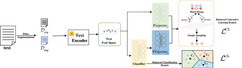
Figure 2: Architecture of SharpReCL (Best viewed in color).

3.1 Preliminaries

Problem Definition: For multiclass TC tasks with $C$ classes, we assume the given dataset $\{x_{i},\ y_{i}\}_{i=1}^{N}$ contains $N$ training examples, where $x_{i}$ is the text sequence and $1\leqslant y_{i}\leqslant C$ is the label assigned to the input text. Our target is to obtain a function $\phi$ mapping from an input space $\mathcal{X}$ to the target space $\mathcal{Y}$. Usually, the function $\phi$ is implemented as the composition of an encoder $\Psi$: $\mathcal{X}$ →$\mathcal{Z}\in\mathbb{R}^{h}$ and a linear classifier $\Omega$: $\mathcal{Z}$ → $\mathcal{Y}$. Our model also adopts this structure.

Contrastive Learning: Given $N$ training samples $\{x_{i}\}_{i=1}^{N}$ and their corresponding augmented samples, each sample has at least one augmented sample in the dataset. For an instance $x_{i}$ and its representation $z_{i}$ in a batch $B$, the standard unsupervised CL loss Chen et al. (2020) can be presented as:

$$\mathcal{L}^{UCL}_{i}=-\frac{1}{|B|}\log\frac{\exp\left(z_{i}\cdot z_{i}^{+}/\tau\right)}{\sum_{k\in B\backslash\{i\}}\exp(z_{i}\cdot z_{k}/\tau)}$$ (1)

where $z_{i}^{+}$ denotes the representation of the augmented sample derived from the $i$-th sample $x_{i}$, and $\tau>0$ is the temperature factor that controls tolerance to similar samples.

SCL treats all samples with the same label in the batch as positive and all other samples as negative. Its loss function can be written as:

$$\mathcal{L}^{SCL}_{i}=\frac{1}{|B_{y}|-1}\sum_{p\in B_{y}\backslash\{i\}}-\log\frac{\exp(z_{i}\cdot z_{p}/\tau)}{\sum_{k\in B\backslash\{i\}}\exp(z_{i}\cdot z_{k}/\tau)}$$ (2)

where $B_{y}$ indicates a subset of $B$ that contains all samples of class $y$.

Analysis: We suppose the distribution of each class in the original dataset of $N$ samples is $\displaystyle\{\pi_{i}\},\ 1\leqslant i\leqslant C$. Generally, the imbalance rate in the dataset can be defined as:

$$ir\ =\frac{\max\{\pi_{i}\}\ }{\min\{\pi_{i}\}\ }\ =\frac{\pi_{max}}{\pi_{min}}$$ (3)

Since SCL works at the sample-pair level, in each batch $B$, we define $P_{i}$ as the number of sample pairs that belong to the same class $i$ and participate in CL. Accordingly, we can define the contrastive imbalance rate as follows:

$$ir^{SCL} =\ \frac{\max\{P_{i}\}}{\min\{P_{i}\}}=\frac{|B|\pi_{max}\cdot(|B|\pi_{max}-1)}{|B|\pi_{min}\cdot(|B|\pi_{min}-1)}$$ (4)

$$\approx\frac{(|B|\pi_{max})^{2}}{(|B|\pi_{min})^{2}}=\left(\frac{\pi_{max}}{\pi_{min}}\right)^{2}={ir}^{2}$$

Thus, we find that when SCL is performed, for every batch, the imbalance ratio becomes the square of the original ratio. Since each epoch consists of many batches, assuming that the sampling in each batch is uniform, the imbalance ratio of each epoch also remains $ir^{2}$. In summary, since SCL works with sample pairs, such a learning mechanism will significantly amplify the class-imbalanced problem in the original data and create more difficulties for model training.

3.2 Overview of SharpReCL

The framework of our model is shown in Fig. 2. Our model consists of two branches, namely, the balanced classification branch and the balanced CL branch. We first apply conventional data augmentation techniques in NLP (such as back-translation Edunov et al. (2018), random noise injection Xie et al. (2017), and word substitution Wei and Zou (2019)) to obtain the augmented data $D_{aug}$ for the original data $D_{org}$. We default to word substitution, and the results of different augmentation methods can be found in Appendix A.1. Here, we denote the texts under two perspectives as $D=D_{org}\cup D_{aug}$. Since PLMs such as BERT have shown their superior representation capability, we use PLMs as the backbone encoder for text samples in SharpReCL. For each text sequence sample $x_{i}$, we first obtain its encoded representations using the encoder, i.e., $feat_{i}=PLM(x_{i})\in\mathbb{R}^{h_{1}}$. Then, the balanced classification branch performs TC with the derived text representations and obtains class prototype vectors. After that, we project these two types of representations into the same space. In this space, the data are expanded by mixup techniques, and then, the balanced CL is performed.

3.3 Balanced Classification Branch for Class Prototype Generation

The prototype vector represents each class and acts as a data complement by becoming an instance of the corresponding class in subsequent operations. In SharpReCL, we use the class-specific weights from the backbone classification branch to represent each class, making the class prototype vectors directly learnable. Moreover, these prototype vectors can be corrected by explicitly utilizing labels in the classification task.

Most classification models typically adopt cross-entropy loss, which is suboptimal on imbalanced data since the label distributions introduce bias into the trained model. These models perform well for instances of the majority class but poorly for instances of the minority class. Logit compensation Menon et al. (2020) is an effective method for imbalanced data that overcomes the shortcomings of the previous reweighting methods and increases the classification boundary between classes based on a simple adjustment of the traditional cross-entropy loss with a class prior. Therefore, we adopt logit compensation instead of the conventional cross-entropy loss in our experiments.

Here, we use a linear function to obtain the class logits, where the weights of the linear function are used as class-specific weights. After the procedure of one projection head $proj_{h}$, we can obtain the prototype vectors. The above operations can be expressed as:

$$\varphi(feat) =w^{T}\cdot feat$$ (5)

$$proto_{1:C} =proj_{h}(w)$$

where $\varphi(feat)\in\mathbb{R}^{N\times C}$ denotes the class logits, and $proto_{1:C}\in\mathbb{R}^{C\times h_{2}}$ represents the class prototype vectors. The projection head $proj_{h}$ is implemented by a two-layer MLP. After obtaining class logits, we perform logit compensation for classification, which can be written as:

$$\mathcal{L}^{CLS}(y,\ \varphi(feat))=-\log\frac{\exp(\varphi_{y}(feat)+\delta_{y})}{\sum_{y^{\prime}\ \in\ [\mathcal{Y}]}\exp(\varphi_{y^{\prime}}(feat)+\delta_{y^{\prime}})}$$ (6)

Here, $\delta_{y}$ stands for the compensation for class $y$, and its value is related to the class-frequency. In SharpReCL, we set the class compensation $\delta_{y}$ to $\log\mathbb{P}_{y}$ , where $\mathbb{P}_{y}$ is the class prior of class $y$.

3.4 Simple-Sampling and Hard-Mixup for the Rebalanced Dataset

We use the feature projection head $proj_{f}$ to map the encoded representations $feat$ of texts such that the texts’ hidden representation $z$ is in the same space as the prototype vector $proto$. For each text-encoded representation $feat_{i}$, this operation can be denoted as:

$$z_{i}\ =\ proj_{f}(feat_{i})$$ (7)

Since prototype vectors are used to represent each class, we address the extreme case where samples from the minority classes do not appear in a batch. This is because we supplement the prototype vectors into each batch of data. We denote the extended dataset as $\hat{D}=\mathbf{Z}\cup proto$ and then perform $l_{2}$-normalization on it, where $\mathbf{Z}$ and $proto$ represent the sets of hidden text vectors and class prototype vectors, respectively. In this section, we further correct the imbalanced dataset by constructing a balanced dataset.

On the one hand, not all samples are helpful for model training, and overly easy samples contribute little to the gradient Robinson et al. (2020); on the other hand, extreme (particularly hard) samples can also lead to performance degradation Song et al. (2022). Therefore, in SharpReCL, we use a combination of simple-sampling and hard-mixup to construct the balanced dataset.

Simple-Sampling: As a natural idea, we need to perform resampling on the dataset to expand it. In SCL, positive samples of each class are samples from the same class, and negative samples are other samples from different classes. Therefore, for each class $c,\ 1\leqslant c\leqslant C$, we can construct its positive sample set $D^{+}$ and negative sample set $D^{-}$ by simply sampling from $\hat{D}$, which can be written as:

$$D_{samp,c}^{+}\ =\ Samp\{z_{i}\},\ z_{i}\ \in\hat{D}\ \wedge\ y_{i}=c$$ (8)

$$D_{samp,c}^{-}\ =\ Samp\{z_{i}\},\ z_{i}\ \in\hat{D}\ \wedge\ y_{i}\neq c$$

where $Samp\{\cdot\}$ denotes the sampling operation.

Hard-Mixup: We use the prototype vectors as a criterion to measure the learning difficulty of the samples to obtain the hard sample set. For each class $c,\ 1\leqslant c\leqslant C$ and its prototype vector $proto_{c}$, we consider the top-k positive samples from class $c$ that are not similar to $proto_{c}$ as hard positive samples, and the top-k negative samples from other classes that are similar to $proto_{c}$ as hard negative samples, which can be denoted as:

$$D_{hard,c}^{+} =\text{top-{k}}\{-proto_{c}\cdot z_{i},z_{i}\},z_{i}\in\hat{D}\ \wedge\ y_{i}=c$$ (9)

$$D_{hard,c}^{-} =\text{top-{k}}\{proto_{c}\cdot z_{i},z_{i}\},z_{i}\in\hat{D}\ \wedge\ y_{i}\neq c$$

To increase sample diversity and to improve learning efficiency, we need to further amplify the hard samples obtained by previous procedures. Mixup and its variants have been proven effective in a series of works Zhang et al. (2018); Yun et al. (2019) as a simple but effective data augmentation method by using interpolation between samples. In SharpReCL, we apply mixup to further augment the data in hard sample sets. This operation is denoted as:

$$D_{syn,c}^{+}=\left\{\frac{\tilde{z}_{k}^{+}}{||\tilde{z}_{k}^{+}||}\right\},\ \tilde{z}_{k}^{+}=\alpha_{k}z_{i}^{+}+(1-\alpha_{k})z_{j}^{+}$$ (10)

$$\ D_{syn,c}^{-}=\left\{\frac{\tilde{z}_{k}^{-}}{||\tilde{z}_{k}^{-}||}\right\},\ \tilde{z}_{k}^{-}=\beta_{k}z_{i}^{-}+(1-\beta_{k})z_{j}^{-}$$

where ($z_{i}^{+},z_{j}^{+}$) and ($z_{i}^{-},z_{j}^{-}$) are randomly sampled from the corresponding hard sample sets $D_{hard,c}^{+}$ and $D_{hard,c}^{-}$, and $\alpha_{k},\beta_{k}\sim Beta\left(\lambda,\lambda\right)$ are in the range of $(0,1)$. By default, we set $\lambda$ to 0.5.

In this way, for each class $c$, we construct a balanced positive sample set $\tilde{D}_{c}^{+}\!=\!D_{samp,c}^{+}\!\cup\!D_{syn,c}^{+}$ and a balanced negative sample set $\tilde{D}_{c}^{-}\!=\!D_{samp,c}^{-}\!\cup\!D_{syn,c}^{-}$. The rebalanced dataset $\tilde{D}$ for all classes can be represented as $\tilde{D}\!=\!\{\tilde{D}_{c}^{+}\!\cup\tilde{D}_{c}^{-}\}_{c}^{C}\!=\!D_{samp}\!\cup D_{syn}$.

3.5 Contrastive Learning Branch with a Rebalanced Dataset

One issue of concern is the control of the ratio of the hard-mixup dataset $D_{syn}=\{D_{syn,c}^{+}\cup D_{syn,c}^{-}\}_{c}^{C}$ to the balanced dataset $\tilde{D}$. Since the feature extraction ability of the model becomes stronger with increasing iterations during the training process, we set the ratio for $D_{syn}$ to $0.5+\frac{t}{T}\times 0.5$, with $t$ being the current number of iterations and $T$ being the total number of iterations. In this way, the difficulty of the balanced sample set we construct is flexible and controllable, which becomes more challenging during the training process and facilitates the training and learning of the model.

Note that we treat the sample pairs in traditional CL as two parts, $i.e.$, the anchor sample and the target sample. The anchor sample comes from the original samples in the batch together with prototype vectors, i.e., $\hat{D}$, and the target sample set consists of $\hat{D}$ and our constructed sample set $\tilde{D}$. Therefore, the original class imbalance problem still exists in the anchor samples.

To alleviate this problem, we add the class prior $\delta$ used in Eq. 6 to the original SCL to correct $\mathcal{L}^{SCL}$ in Eq. 2 based on the idea of reweighting. The concrete objective function can be written as:

$$\mathcal{L}^{CL}_{i}\!=-\frac{\delta_{y}}{|\hat{D}|} \!\sum_{p\!\in\tilde{D}_{y}^{+}\!\cup\hat{D}_{y}\!\backslash\{i\}}\!-\!\log\frac{\exp(z_{i}\cdot z_{p}/\tau)}{\!\sum\limits_{k\!\in\tilde{D}_{y}\!\cup\hat{D}\!\backslash\{i\}}\exp(z_{i}\cdot z_{k}/\tau)}$$ (11)

$$\mathcal{L}^{CL} =\ \sum_{i\in\hat{D}}\mathcal{L}_{i}^{CL}$$

The generation of hard samples can alleviate the issue of vanishing gradients and is beneficial for CL training, as supported by mathematical analysis in Appendix A.2.

Finally, we have the following loss for training:

$$\mathcal{L}^{overall}=\mathcal{L}^{CLS}\ +\ \mu\mathcal{L}^{CL}$$ (12)

where $\mu$ is the hyperparameter that controls the impact of CL branch, and this branch only intends for the backbone to learn the desired feature embeddings. We feed the obtained test text embeddings to the classification branch during the model inference stage to evaluate the model performance.

The concrete training procedure of our model can be found in Algorithm 1.

Algorithm 1 SharpReCL Training

Input: The text dataset $D=D_{org}\cup D_{aug}=\{x_{i},y_{i}\}_{i}^{2N}$, the text encoder $PLM(\cdot)$, the linear function $\varphi(\cdot)$, projection heads $proj_{f}(\cdot)$ and $proj_{h}(\cdot)$

1:  Initialize the network parameters

2:  for $t=1,2,\dots,T$  do

3:     Obtain texts’ encoded embeddings $feat$ using $PLM(\cdot)$

4:     Obtain the class logits and prototype vectors $proto$ with $\varphi(\cdot)$ and $proj_{h}(\cdot)$ in Eq.5

5:     Obtain the hidden embeddings of texts with $proj_{f}(\cdot)$ in Eq.7

6:     Compute $|D_{samp}|$ and $|D_{syn}|$

7:     Perform Simple-Samping to obtain $D_{samp}$ with Eq.8

8:     Perform Hard-Mixup to obtain $D_{hard}$ with Eq.9

9:     Apply Mixup techniques to obtain $D_{syn}$ with Eq.10

10:     Obtain the re-balanced dataset $\tilde{D}=D_{samp}\cup D_{syn}$

11:     Compute the classification loss $\mathcal{L}^{CLS}$ with Eq.6

12:     Compute the CL loss $\mathcal{L}^{CL}$

13:     Compute the overall loss $\mathcal{L}^{overall}$ with Eq.12

14:     Optimize the model by backpropagation of $\mathcal{L}^{overall}$

15:  end for

Output: The well-trained SharpReCL

4 Experiments

Datasets: We employ six widely used real-world datasets to evaluate the effectiveness of our model, where the train/test split of datasets is the same as previous studies Tang et al. (2015). They are R52 Liu et al. (2021), Ohsumed Yao et al. (2019), TREC Li and Roth (2002), DBLP Tang et al. (2015), Biomedical Xu et al. (2017), and CR Ding et al. (2008), with detailed descriptions provided in Appendix A.3. The detailed statistics of these datasets are summrized in Table 1. We use the original R52 and Ohsumed datasets directly, since they are extremely imbalanced. Other datasets are relatively balanced. There is only one category in the TREC with few samples. Thus the calculated $ir$ is large, but we still treat it as a balanced dataset, which needs preprocessing. We create the imbalanced version of balanced datasets by reducing the training samples of each sorted class with a deterministic $ir$, which is a common practice in imbalanced learning Cui et al. (2019). For example, if we set $ir$ to 10, the number of each category in a balanced dataset with three categories is 1000, 900, and 890, each category in the imbalanced version is 1000, 100, and 10.

Dataset	#Train	#Test	#Word	Avg. Len	#Class	$ir$
R52	6,532	2,568	8,892	69.82	52	1307.7
Ohsumed	3,353	4,043	14,157	135.82	23	65.0
TREC	5,452	500	8,751	11.3	6	14.5
DBLP	61,422	20,000	22.27	8.5	6	4.0
Biomedical	17,976	1,998	18,888	12.88	20	1.1
CR	3,394	376	5,542	18.2	2	1.8

Table 1: Detailed statistics of the evaluation datasets.

Baselines: We compare the proposed model with the following three types of competitive baselines. Pretrained language models and their imbalanced learning versions include BERT Devlin et al. (2019), BERT+Dice Loss Li et al. (2020b), BERT+Focal Loss Lin et al. (2017), and RoBERTa Liu et al. (2019). Contrastive learning models contain SimCSE Gao et al. (2021), SCLCE Gunel et al. (2021), SPCL Song et al. (2022), and DualCL Chen et al. (2022). Large language models consist of GPT-3.5 Ouyang et al. (2022), Bloom-7.1B Scao et al. (2022), Llama2-7B Touvron et al. (2023), and Llama3-8B AI@Meta (2024). Due to computational resource constraints, we only fine-tune approximately 7B LLMs through some GPU reduction techniques. The detailed descriptions of baselines are provided in Appendix A.4. Moreover, the implementation details are placed in Appendix A.5. To accelerate the model training, we use the 24GB Nvidia GeForce RTX 3090Ti GPU.

Evaluation Metrics: We employ the accuracy (Acc) and macro-f1 score (F1) to examine all the models’ performance. All experiments are conducted ten times to obtain average metrics for statistical significance.

5 Results

Dataset	ir	Metric	BERT	BERT+ Dice Loss	BERT+ Focal Loss	RoBERTa	SimCSE	SCLCE	SPCL	DualCL	GPT-3.5	Bloom-7.1B	Llama2-7B	Llama3-8B	Ours
R52	org	Acc	95.55$\pm$0.36	95.48$\pm$0.29	95.66$\pm$0.25	95.56$\pm$0.22	89.35$\pm$0.20	95.51$\pm$0.35	94.29$\pm$0.36	94.16$\pm$0.16	95.27$\pm$0.55	OOM	OOM	OOM	96.11$\pm$0.36
		F1	82.88$\pm$0.28	81.58$\pm$0.32	83.72$\pm$0.26	82.33$\pm$0.35	79.22$\pm$0.15	83.64$\pm$0.39	83.19$\pm$0.32	73.92$\pm$0.12	79.15$\pm$0.52	OOM	OOM	OOM	84.83$\pm$0.29
Ohsumed	org	Acc	65.71$\pm$0.30	65.94$\pm$0.20	65.22$\pm$0.26	66.06$\pm$0.23	49.30$\pm$0.32	66.59$\pm$0.35	67.20$\pm$0.42	26.44$\pm$0.35	51.84$\pm$0.45	67.54$\pm$0.62	67.66$\pm$0.72	68.02$\pm$0.26	68.44$\pm$0.22
		F1	57.36$\pm$0.31	55.59 $\pm$0.36	55.00$\pm$0.28	56.95$\pm$0.26	36.00$\pm$0.40	56.25$\pm$0.39	56.42$\pm$0.42	14.75$\pm$0.55	43.83$\pm$0.65	53.52$\pm$0.72	55.92$\pm$0.69	58.59$\pm$0.19	60.82$\pm$0.20
TREC	org∗	Acc	97.60$\pm$0.39	97.60$\pm$0.42	97.20$\pm$0.56	97.61$\pm$0.55	88.80$\pm$0.62	97.60$\pm$0.38	96.50$\pm$0.95	97.80$\pm$1.25	96.20$\pm$1.55	96.60$\pm$1.65	97.62$\pm$1.62	97.00$\pm$1.15	97.20$\pm$0.95
		F1	96.99$\pm$0.52	96.97$\pm$0.55	96.13$\pm$0.65	97.00$\pm$0.62	85.90$\pm$0.72	97.01$\pm$0.42	95.50$\pm$1.20	97.38$\pm$1.72	95.62$\pm$1.82	94.36$\pm$1.96	97.09$\pm$1.92	96.50$\pm$1.22	97.63$\pm$0.82
	50	Acc	93.40$\pm$0.66	93.60$\pm$0.50	94.40$\pm$0.52	92.60$\pm$0.39	74.00$\pm$0.29	94.20$\pm$0.30	93.52$\pm$1.25	92.80$\pm$1.55	94.66$\pm$1.93	94.40$\pm$1.76	95.00$\pm$2.25	94.50$\pm$0.65	94.80$\pm$0.55
		F1	93.30 $\pm$ 0.65	92.36 $\pm$ 0.69	94.26 $\pm$ 0.40	92.50 $\pm$ 0.41	76.00$\pm$0.32	93.97$\pm$0.39	92.40$\pm$1.52	91.05$\pm$1.62	93.52$\pm$2.02	93.00$\pm$2.12	93.46$\pm$2.29	93.80$\pm$0.59	94.83$\pm$0.52
	20	Acc	96.60 $\pm$0.49	96.60$\pm$0.28	95.80$\pm$0.46	96.60$\pm$0.53	82.20$\pm$0.35	96.80$\pm$0.60	95.52$\pm$0.62	96.40$\pm$1.79	96.69$\pm$2.35	96.90$\pm$2.39	96.60$\pm$2.06	96.40$\pm$0.62	97.00$\pm$0.52
		F1	96.05$\pm$0.56	96.25$\pm$0.19	95.53$\pm$0.55	95.31$\pm$0.52	82.00$\pm$0.38	96.32$\pm$0.71	94.19$\pm$0.63	95.25$\pm$1.59	95.56$\pm$1.99	96.25$\pm$2.25	96.17$\pm$2.42	94.31$\pm$0.26	96.45$\pm$0.21
	10	Acc	96.60$\pm$0.42	97.00$\pm$0.30	96.80$\pm$0.27	97.00$\pm$0.24	85.00$\pm$0.25	97.00$\pm$0.72	96.70$\pm$0.75	97.60$\pm$1.66	96.62$\pm$1.25	97.40$\pm$2.12	96.80$\pm$1.62	95.20$\pm$1.66	97.20$\pm$0.35
		F1	95.38$\pm$0.55	95.99$\pm$0.37	96.41$\pm$0.29	96.55$\pm$0.46	82.20$\pm$0.70	95.64$\pm$0.82	95.72$\pm$0.71	97.34$\pm$1.72	96.26$\pm$1.52	96.89$\pm$2.22	96.32$\pm$1.55	93.59$\pm$1.35	97.53$\pm$0.39
DBLP	org∗	Acc	79.62 $\pm$0.66	80.09 $\pm$0.38	79.73 $\pm$0.53	79.85 $\pm$0.32	68.50$\pm$0.39	79.96$\pm$0.59	79.85$\pm$0.66	80.52$\pm$1.73	78.96$\pm$1.55	81.76$\pm$2.05	82.20$\pm$0.85	83.21$\pm$0.79	80.15$\pm$0.39
		F1	76.47$\pm$0.18	77.27$\pm$0.15	76.57$\pm$0.25	76.99$\pm$0.45	64.40$\pm$0.23	76.84$\pm$0.60	77.20$\pm$0.68	77.67$\pm$1.22	78.06$\pm$1.29	78.08$\pm$2.39	78.70$\pm$1.25	80.12$\pm$1.59	77.59$\pm$0.28
	50	Acc	74.53$\pm$0.38	74.34$\pm$0.39	73.94$\pm$0.42	74.19$\pm$0.53	62.40$\pm$0.30	74.49$\pm$0.90	74.96$\pm$0.78	75.72$\pm$1.85	75.29$\pm$1.88	76.60$\pm$2.19	77.50$\pm$2.22	78.00$\pm$2.15	76.30$\pm$0.25
		F1	68.60$\pm$0.32	67.20$\pm$0.45	67.99$\pm$0.39	67.03$\pm$0.59	51.30$\pm$0.33	67.75$\pm$0.92	67.70$\pm$0.87	69.57$\pm$1.99	70.22$\pm$2.02	70.10$\pm$2.32	71.30$\pm$2.55	71.20$\pm$2.19	71.15$\pm$0.36
	20	Acc	77.20$\pm$0.93	76.95$\pm$0.65	77.11$\pm$0.16	76.70$\pm$0.29	65.10$\pm$0.35	77.65$\pm$0.26	77.72$\pm$0.73	78.20$\pm$2.01	79.12$\pm$2.11	80.40$\pm$1.88	80.62$\pm$2.16	80.92$\pm$1.96	78.72$\pm$0.31
		F1	72.93$\pm$1.11	72.69$\pm$0.68	72.71$\pm$0.23	72.15$\pm$0.35	57.00$\pm$0.39	73.16$\pm$0.30	73.12$\pm$0.76	74.07$\pm$1.98	74.16$\pm$2.18	76.10$\pm$1.93	76.25$\pm$2.55	76.75$\pm$2.65	75.13$\pm$0.38
	10	Acc	78.86$\pm$0.99	78.35$\pm$0.82	78.70$\pm$0.36	78.21$\pm$0.39	67.10$\pm$0.38	78.96$\pm$0.86	78.42$\pm$0.77	79.03$\pm$2.66	78.52$\pm$2.39	80.92$\pm$2.08	80.22$\pm$2.60	81.26$\pm$2.60	79.59$\pm$0.41
		F1	75.16$\pm$1.22	74.78$\pm$0.89	75.30$\pm$0.32	74.52$\pm$0.55	61.00$\pm$0.42	75.92$\pm$0.88	75.42$\pm$0.79	75.81$\pm$2.72	76.52$\pm$2.42	77.42$\pm$2.11	77.06$\pm$2.69	77.75$\pm$0.46	76.75$\pm$0.46
Biomedical	org∗	Acc	71.22$\pm$0.82	70.76$\pm$0.73	70.59$\pm$0.30	70.78$\pm$0.62	62.80$\pm$0.29	71.42$\pm$0.60	70.92$\pm$0.66	70.90$\pm$1.89	71.52$\pm$2.30	72.90$\pm$2.09	72.39$\pm$2.51	73.58$\pm$2.10	72.52$\pm$0.39
		F1	71.10$\pm$0.86	70.69 $\pm$ 0.75	70.32$\pm$0.39	70.56$\pm$0.65	61.85$\pm$0.32	71.32$\pm$0.75	69.39$\pm$0.72	70.81$\pm$1.92	71.66$\pm$2.39	73.02$\pm$2.19	72.50$\pm$2.59	73.65$\pm$2.01	72.65$\pm$0.26
	50	Acc	59.17$\pm$0.56	59.32$\pm$0.79	55.52$\pm$0.19	58.14$\pm$0.51	58.22$\pm$0.33	59.28$\pm$1.01	60.16$\pm$0.69	59.42$\pm$1.90	55.79$\pm$2.51	52.10$\pm$2.30	55.92$\pm$2.22	54.40$\pm$2.29	61.56$\pm$0.28
		F1	57.72$\pm$0.55	58.89$\pm$0.82	53.76$\pm$0.20	57.44$\pm$0.55	56.45$\pm$0.36	58.45$\pm$1.09	59.05$\pm$0.89	58.72$\pm$1.99	52.62$\pm$2.66	48.10$\pm$2.55	55.85$\pm$2.02	49.32$\pm$2.02	60.78$\pm$0.12
	20	Acc	64.42$\pm$0.35	64.48$\pm$0.63	62.67$\pm$0.29	62.82$\pm$0.66	54.50$\pm$0.26	64.37$\pm$0.15	64.19$\pm$0.39	63.65$\pm$1.93	61.26$\pm$2.18	60.32$\pm$1.86	63.55$\pm$2.11	57.40$\pm$1.95	65.47$\pm$0.22
		F1	64.09$\pm$0.31	64.06$\pm$0.56	61.92$\pm$0.22	62.24$\pm$0.72	54.30$\pm$0.30	63.96$\pm$0.21	63.49$\pm$0.28	63.06$\pm$1.99	60.25$\pm$2.03	58.16$\pm$2.05	62.96$\pm$2.19	55.30$\pm$1.96	64.83$\pm$0.26
	10	Acc	66.90$\pm$0.39	66.74$\pm$0.70	66.39$\pm$0.35	66.73$\pm$0.82	58.20$\pm$0.30	66.81$\pm$0.66	66.10$\pm$0.58	66.45$\pm$0.86	63.26$\pm$2.11	65.80$\pm$2.09	66.62$\pm$1.99	62.32$\pm$1.90	68.11$\pm$0.60
		F1	66.97$\pm$0.31	66.69$\pm$0.69	66.32$\pm$0.36	66.52$\pm$0.89	58.30$\pm$0.39	66.77$\pm$0.69	64.92$\pm$0.66	66.50$\pm$0.90	63.19$\pm$1.98	65.02$\pm$2.26	66.22$\pm$2.05	62.82$\pm$0.55	68.06$\pm$0.55
CR	org∗	Acc	92.02$\pm$0.56	92.26$\pm$0.29	91.02$\pm$0.39	92.55$\pm$0.72	86.05$\pm$0.26	91.22$\pm$0.16	91.55$\pm$0.26	92.65$\pm$0.77	90.16$\pm$2.05	92.55$\pm$2.11	94.41$\pm$2.09	94.70$\pm$0.35	93.09$\pm$0.30
		F1	91.39$\pm$0.59	91.60$\pm$0.19	91.30$\pm$0.36	92.03$\pm$0.77	85.92$\pm$0.32	90.62$\pm$0.22	91.36$\pm$0.28	92.16$\pm$0.79	89.02$\pm$2.29	92.01$\pm$2.19	93.03$\pm$2.16	93.70$\pm$0.62	92.51$\pm$0.22
	50	Acc	77.39$\pm$1.01	80.59$\pm$0.26	77.93$\pm$0.55	78.99$\pm$0.56	77.90$\pm$0.31	79.69$\pm$0.18	80.25$\pm$0.25	77.13$\pm$0.70	80.55$\pm$2.06	82.71$\pm$2.19	83.92$\pm$1.95	80.59$\pm$1.22	84.04$\pm$0.25
		F1	70.38$\pm$1.06	75.37$\pm$0.32	70.67$\pm$0.56	73.83$\pm$0.59	71.10$\pm$0.35	74.46$\pm$0.22	75.62$\pm$0.30	69.50$\pm$0.72	78.29$\pm$2.02	78.46$\pm$2.25	80.41$\pm$2.15	75.22$\pm$1.02	81.12$\pm$0.26
	20	Acc	84.04$\pm$0.39	83.24$\pm$0.55	84.04$\pm$0.62	80.59$\pm$0.22	81.90$\pm$0.31	85.69$\pm$0.35	85.42$\pm$0.55	88.83$\pm$0.60	89.55$\pm$1.79	90.76$\pm$1.99	90.96$\pm$1.95	89.36$\pm$0.56	89.36$\pm$0.50
		F1	80.51$\pm$0.36	79.48$\pm$0.56	80.83$\pm$ 0.65	75.37$\pm$0.23	77.40$\pm$0.36	83.35$\pm$0.36	82.56$\pm$0.59	87.20$\pm$0.66	89.22$\pm$1.85	89.60$\pm$2.02	89.73$\pm$2.15	87.81$\pm$0.55	88.28$\pm$0.52
	10	Acc	86.44$\pm$0.22	88.30$\pm$0.26	90.69$\pm$0.60	90.16$\pm$0.66	83.80$\pm$0.28	88.28$\pm$0.31	89.15$\pm$0.52	90.43$\pm$0.70	91.09$\pm$2.10	92.29$\pm$1.75	92.02$\pm$2.16	93.35$\pm$0.66	90.96$\pm$0.16
		F1	84.29$\pm$0.25	86.60$\pm$0.30	89.53$\pm$0.55	88.94$\pm$0.69	80.70$\pm$0.32	87.29$\pm$0.39	88.25$\pm$0.55	89.38$\pm$0.79	90.56$\pm$2.19	91.43$\pm$1.89	91.08$\pm$2.11	92.66$\pm$0.59	90.21$\pm$0.26

Table 2: The results (%) of Acc and Macro-F1 scores of various experimental settings. The performance of our model is a statistically significant improvement over the best baseline, with a p-value smaller than 0.001. “org^∗” represents the case where the classes are relatively balanced. Underline: runner-up. OOM: out of memory.

Model Performance: We perform extensive experiments on our model and other competitive baselines with six public datasets under different imbalanced settings, including original data, $ir$=50, $ir$=20 and $ir$=10. We present the experimental results in Table 2. Based on the quantitative results, we gain in-depth insights and analyses. First, our model significantly outperforms other baselines in most imbalanced experimental settings, illustrating its superiority in modeling imbalanced text data. An important reason is that SharpReCL introduces class prototypes during training, which ensures that all classes appear in every batch, effectively resolving the problem of missing minority classes due to data sampling. Meanwhile, we introduce hard positive and hard negative samples for each class in SCL, which can provide more adequate gradients and thus facilitate model optimization. Based on this, we generate a balanced contrastive queue for each class by using the mixup technique, which effectively alleviates the previous issue that the majority categories dominate the training process in an imbalanced dataset.

We find other models achieve inferior performance due to serious bias in representation learning. Notably, our model achieves the best performance on several datasets (such as Ohsumed and Biomedical) even when compared to LLMs. One plausible reason is that LLMs lack sufficient domain-specific training data, leading to their inadequate understanding of these texts. On the other hand, they may encounter data leakage problem, meaning they have already seen the test data. Additionally, according to Table 3, SharpReCL significantly outperforms LLMs in terms of training and inference efficiency across all datasets due to its fewer trainable parameters.

Model	Ohsumed		TREC		DBLP		Biomedical		CR
	Train	Inference	Train	Inference	Train	Inference	Train	Inference	Train	Inference
Bloom-7.1B	3,479	1,143	3,493	71	37,524	2,417	8,430	2,109	910	48
Llama2-7B	1,480	1,481	1,712	98	40,783	2,628	13,017	946	898	72
Llama3-8B	2,507	13,14	2,628	75	28,966	2,753	9,833	1,044	1,646	54
Ours	21	3	16	0.56	129	9	310	22	44	0.89

Table 3: Time-consuming (s) for training one epoch and inference across several evaluation datasets varies for different models.

Model	R52		Ohsumed		TREC		DBLP		Biomedical		CR
	Acc	F1	Acc	F1	Acc	F1	Acc	F1	Acc	F1	Acc	F1
w/o SSHM	94.59	82.93	66.59	56.25	94.20	93.97	74.49	67.75	59.28	58.45	79.69	74.46
w/o CL	95.09	83.52	66.86	57.52	94.40	93.30	74.65	68.04	59.44	58.98	77.39	69.75
w/o CLS	95.62	83.95	66.89	57.56	94.42	93.99	74.69	68.22	59.66	60.02	78.59	72.16
w/o SS	95.66	83.99	67.28	59.13	93.80	84.88	75.53	71.43	61.35	60.72	80.05	75.15
w/o HM	95.69	84.05	67.55	59.95	94.00	93.99	75.44	70.78	60.92	60.52	82.78	80.18
Ours	96.11	84.83	68.44	60.82	94.80	94.83	76.30	71.15	61.56	60.78	84.04	81.12

Table 4: The results of ablation studies on our model.

Ablation Study: To evaluate the individual effects of the proposed SharpReCL, we perform a series of ablation experiments on all datasets except Ohsumed with an imbalance ratio of 50. We use the original Ohsumed dataset. Specifically, w/o SSHM removes the simple-sampling and hard-mixup module, which simply incorporates the cross-entropy and CL objective. w/o SS and w/o HM delete the simple-sampling module and hard-mixup module, respectively. w/o CL excludes the CL branch and leaves the classification branch. w/o CLS eliminates the classification branch, which is evaluated with a linear classifier by frozen representations trained via CL. The results are presented in Table 4. We observe that each component of SharpReCL is indispensable and that removing any of the components degrades the performance. The first variant has the most significant performance degradation because the imbalanced class distribution in a batch makes the model learn biased text representations. The fourth and fifth variants show that simple-sampling and hard-mixup modules are critical for the quality of the rebalanced dataset. Removing the CL branch drastically reduces the ability of the model to extract invariant knowledge from similar texts. We explore more ablation experiments in Appendix A.6.

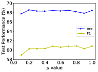
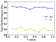
Figure 3: Hyperparameter sensitivity of our model on Ohsumed. Other datasets are placed in Appendix A.7, omitted for space.

Parameter Sensitivity: We investigate the sensitivity of the model with respect to primary hyperparameters on the Ohsumed dataset, i.e., the controlled weight for contrastive loss $\mu$ and the temperature $\tau$. From Fig. 3, we find that the model is insensitive to the parameter $\mu$ from 0.2 to 1, illustrating its robustness. Moreover, the accuracy of the model is relatively stable across different selections of $\tau$ from [0.1, 1], while the F1 scores vary drastically depending on different $\tau$. If the $\tau$ value is set too low, it causes the model to excessively prioritize hard negative samples. At the same time, a too high $\tau$ value causes the model to treat all samples equally, both compromising learned semantic information.

Moreover, due to the space constraints, we present additional experiments in Appendix A.8.

6 Conclusion

In this work, we propose a novel model, namely, SharpReCL, for imbalanced TC tasks based on SCL. We make the classification branch and the SCL branch communicate and guide each other by leveraging learned prototype vectors. To address the sensitivity of SCL to class imbalance, we construct a balanced dataset consisting of hard negative and hard positive samples by using the mixup technique to balance the sample pairs for SCL training. Extensive experiments on several datasets under different imbalanced settings demonstrate the effectiveness of our model.

Appendix

Dataset	R52		Ohsumed		TREC		DBLP		Biomedical		CR
	Acc	F1	Acc	F1	Acc	F1	Acc	F1	Acc	F1	Acc	F1
Word substitution	96.11	84.83	68.44	60.82	97.20	97.63	80.15	77.59	72.52	72.65	93.09	92.51
Back translation	95.92	84.69	68.09	59.41	97.20	96.84	80.12	77.22	72.83	72.87	93.09	92.58
Contextual embedding	96.05	84.76	67.62	59.20	97.80	97.18	80.14	77.38	72.61	72.61	93.09	92.54

Table 5: The results of different augmentations on all original datasets.

A.1 The Impacts of Different Data Augmentations

To investigate the impacts of different data augmentations on the model, we implement the following three methods. (I) Word substitution: We use synonyms from WordNet to replace associated words in the input text. (II) Back translation: We first translate the input text into another language (French), and then translate it back into English to generate a paraphrased version of the input text. (III) Contextual embedding: We use pre-trained LMs to find the top-n most suitable words in the input text for insertion. Based on the results shown in Table 5, we can observe that all data augmentation methods can achieve desirable results. However, there is no universal method that can perform optimally on all datasets, as the optimal configuration of data augmentation methods varies depending on the dataset.

A.2 Mathematical Analysis with Hard Samples

$$\mathcal{L}^{CL}_{i}\!=-\frac{\delta_{y}}{|\hat{D}|} \!\sum_{p\!\in\tilde{D}_{y}^{+}\!\cup\hat{D}_{y}\!\backslash\{i\}}\!-\!\log\frac{\exp(z_{i}\cdot z_{p}/\tau)}{\!\sum\limits_{k\!\in\tilde{D}_{y}\!\cup\hat{D}\!\backslash\{i\}}\exp(z_{i}\cdot z_{k}/\tau)}$$ (13)

$$\mathcal{L}^{CL} =\ \sum_{i\in\hat{D}}\mathcal{L}_{i}^{CL}$$

For the used supervised contrastive loss as shown in Eq. 13, we can obtain the gradient of $\mathcal{L}_{i}^{CL}$ with respect to node embeddings $z_{k}$ as follows:

$$\frac{\partial\mathcal{L}_{i}^{CL}}{\partial z_{i}}=\frac{1}{\tau}\bigl{[}\sum_{p\!\in\tilde{D}_{y}^{+}\!\cup\hat{D}_{y}\!\backslash\{i\}}z_{p}(P_{i,p}-\frac{1}{|\hat{D}|})$$ (14)

$$+\sum_{k\!\in\tilde{D}_{y}^{-}\!\cup\hat{D}\!\backslash\{i\cup\hat{D}_{y}\}}z_{k}P_{i,k}\bigr{]}$$

$$P_{i,k}=\frac{\exp(z_{i}\cdot z_{k}/\tau)}{\sum\limits_{k\!\in\tilde{D}_{y}\!\cup\hat{D}\!\backslash\{i\}}\exp(z_{i}\cdot z_{k}/\tau)}$$

According to Eq. 14, the gradient of $\mathcal{L}_{k}$ with respect to $z_{k}$ consists of two parts. The first part is the gradient provided by positive sample pairs, and the second part is the gradient provided by negative sample pairs. When positive pairs are simple, it causes $P_{i,p}\rightarrow\frac{1}{|\hat{D|}}$, whereas when negative pairs are particularly simple, it causes $P_{i,k}\rightarrow 0$. Both scenarios can lead to gradient vanishing, causing unstable model training and damaging the learning process of the entire model.

However, we only generate hard positive and negative samples, thus providing larger gradients for the contrastive objective. It helps prevent the aforementioned cases and promotes more stable model training.

A.3 Detailed Descriptions of Datasets

R52 Liu et al. [2021] is a dataset containing news articles of 52 categories from Reuters for news classification. Ohsumed Yao et al. [2019] contains many important medical studies and a bibliographic classification dataset. TREC Li and Roth [2002] is a question classification dataset that includes six categories of questions. DBLP Tang et al. [2015] consists of six diverse kinds of paper titles extracted from computer science bibliographies. Biomedical Xu et al. [2017] is a collection of biomedical paper titles that is used for topic classification. CR Ding et al. [2008] is a customer review dataset for sentiment analysis, where the reviews are labeled positive or negative.

A.4 Detailed Descriptions of Baselines

Pretrained language models and their imbalanced learning versions: (I) BERT Devlin et al. [2019] is trained with a large-scale corpus and encodes implicit semantic information. (II) BERT+Dice Loss Li et al. [2020b] uses BERT to encode texts and the Dice loss for optimization. The Dice method dynamically adjusts the weights according to the learning difficulty of the input samples. (III) BERT+Focal Loss Lin et al. [2017] combines BERT, which learns text features, with Focal loss, which offers small scaling factors for predicted classes with high confidence. (IV) RoBERTa Liu et al. [2019] is an enhanced version of BERT that utilizes more training data and large batch sizes.

Contrastive learning models: (I) SimCSE Gao et al. [2021] uses two dropout operations in an unsupervised manner and sentence labels in a supervised manner to generate positive sample pairs. (II) SCLCE Gunel et al. [2021] combines the SCL objective with cross-entropy in the fine-tuning stage of NLP classification models. (III) SPCL Song et al. [2022] attempts to address the class-imbalanced task by combining CL and curriculum learning. (IV) DualCL Chen et al. [2022] solves TC tasks via a dual CL mechanism, which simultaneously learns the input text features and the classifier parameters.

Large language models: (I) GPT-3.5 Ouyang et al. [2022] leverages a vast amount of texts for self-supervised learning and incorporates reinforcement learning with human feedback techniques to fine-tune the pretrained model. (II) Bloom-7.1B Scao et al. [2022] is a decoder-only Transformer language model trained on the ROOTS corpus, and exhibits enhanced performance after being fine-tuned with multi-task prompts. (III) Llama2-7B Touvron et al. [2023] is also a decoder-only large language model that is trained on a new mixup of data from public dataset. It also increases the size of the pretraining corpus by 40%, doubles the model’s context length, and employs grouped query attention. (IV) Llama3-8B AI@Meta [2024] is also an auto-regressive language model, adopting a similar model architecture to Llama2. The main difference lies in its pretraining on a dataset containing over 15T tokens.

A.5 Implementation Details

In the SharpReCL, we utilize the pre-trained BERT base-uncased model as the text encoder by using AdamW with a learning rate of 5e-5. The weight decay and batch size are set to 5e-4 and 128, respectively. We implement the projection head by an MLP with one hidden layer activated by ReLU. The temperature $\tau$ of SCL is chosen from {0.3, 0.5, 1}. Moreover, the number of hard positive and hard negative samples per class in Eq.9 is uniformly 20, i.e., $|D_{hard,c}^{+}|=|D_{hard,c}^{-}|=20$. The number of generated rebalanced positive and negative samples when using mixup for each class $c$ are 10 and 500, i.e., $\tilde{D}_{c}^{+}=10$ and $\tilde{D}_{c}^{-}=500$. The parameter $\mu$ for controlling the loss function is 1. We implement our model with PyTorch 1.10 with Python 3.7.

For SimCSE, similar to SCLCE, we use a linear combination of unsupervised CL loss and CE loss to fully utilize the labeled data for model training. For RoBERTa, we adopt the RoBERTa-base version. We fine-tune GPT-3.5 using the training data from the evaluation dataset through the fine-tuning interface provided by OpenAI, and obtained text classification results using the prompts in Table 6. For Bloom-7.1B, Llama2-7B, and Llama3-8B, we perform full-scale fine-tuning using the training data. To reduce GPU memory usage, we employ LoRA Hu et al. [2021] and 4-bit quantization techniques through the Parameter-Efficient Fine-Tuning (PEFT) method provided by Hugging Face. The prompts used for text classification in Bloom-7.1B, Llama2-7B, and Llama3-8B are the same as those used for GPT-3.5. For other remaining baselines, we use the open-source codes and adopt the parameters suggested by their original papers.

Dataset	Prompts
Ohsumed	Classify the medical research title into one of the 23 classes: {Bacterial Infections and Mycoses, Virus Diseases, Parasitic Diseases, Neoplasms, Musculoskeletal Diseases, Digestive System Diseases, Stomatognathic Diseases, Respiratory Tract Diseases, Otorhinolaryngologic Diseases, Nervous System Diseases, Eye Diseases, Urologic and Male Genital Diseases, Female Genital Diseases and Pregnancy Complications, Cardiovascular Diseases, Hemic and Lymphatic Diseases, Neonatal Diseases and Abnormalities, Skin and Connective Tissue Diseases, Nutritional and Metabolic Diseases, Endocrine Diseases, Immunologic Diseases, Disorders of Environmental Origin, Animal Diseases, Pathological Conditions, Signs and Symptoms}.
TREC	Classify questions into one of five classes: {description, entity, abbreviation, human, location, numeric}.
Biomedical	Classify the biomedical paper titles into one of 18 classes: {aging, chemistry, cats, erythrocytes, glucose, potassium, lung, lymphocytes, spleen, mutation, skin, norepinephrine, insulin, prognosis, risk, myocardium, sodium, mathematics, swine, temperature}.
CR	Classify the customer reviews into negative or positive.

Table 6: Examples of prompts used for different datasets.

Dataset	R52		Ohsumed		TREC		DBLP		Biomedical		CR
	Acc	F1	Acc	F1	Acc	F1	Acc	F1	Acc	F1	Acc	F1
w/o $\delta_{\{\text{CLS,CL}\}}$	95.32	84.33	67.86	60.22	94.40	94.43	75.39	70.05	60.82	60.32	83.49	80.51
w/o $\delta_{\text{CLS}}$	95.79	84.59	68.19	60.46	94.46	94.55	75.52	70.26	60.93	60.46	83.52	80.68
w/o $\delta_{\text{CL}}$	95.95	84.65	68.22	60.52	94.68	94.62	75.64	70.68	61.36	60.59	83.75	80.90
Ours	96.11	84.83	68.44	60.82	94.80	94.83	76.30	71.15	61.56	60.78	84.04	81.12

Table 7: The ablation results of several model variants on all datasets.

Dataset	R52		Ohsumed		TREC		DBLP		Biomedical		CR
	Acc	F1	Acc	F1	Acc	F1	Acc	F1	Acc	F1	Acc	F1
Ours	96.11	84.83	68.44	60.82	97.20	97.63	80.15	77.59	72.52	72.65	93.09	92.51
Ours+Dice	96.19	84.76	68.36	60.76	97.10	97.52	80.22	77.66	72.30	72.59	93.19	92.62
Ours+Focal	96.22	84.85	68.66	60.89	97.12	97.55	80.05	77.52	72.39	72.55	92.92	92.39

Table 8: The results of models with different classifier loss.

A.6 More Ablation Explorations

In our model, as shown in Eq.6 for the classification branch and Eq.12 for the CL branch, we use the class prior $\delta$ to alleviate the imbalance issue of the original samples. To demonstrate the role of the introduced class prior $\delta$, we conduct the following supplementary experiments by designing several model variants under $ir=50$ on all datasets except R52 and Ohsumed. (I) w/o $\delta_{\{\text{CLS,CL}\}}$ removes the class priors $\delta$ from both the classification branch shown in Eq.6 and the CL branch shown in Eq.12. (II) w/o $\delta_{\text{CLS}}$ removes the class prior $\delta$ in classification branch. (III) w/o $\delta_{\text{CL}}$ eliminates the class prior $\delta$ in the CL branch. We present the results of all datasets under $ir=50$ in Table 7. We can observe that the class priors in both the classification branch and CL branch play certain roles, and this is consistent with our expectations. A reasonable explanation is that by introducing class priors, the model’s punishment for misclassifying minor class samples can be increased, causing the model to pay more attention to these misclassified samples.

A.7 Hyperparameter Sensitivity

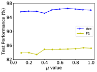
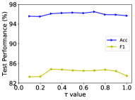
Figure 4: Hyperparameter sensitivity of our model on R52.

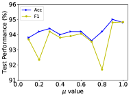
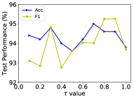
Figure 5: Hyperparameter sensitivity of our model on TREC under $ir$=50.

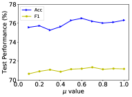
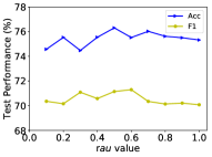
Figure 6: Hyperparameter sensitivity of our model on DBLP under $ir$=50.

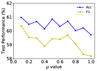
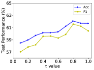
Figure 7: Hyperparameter sensitivity of our model on Biomedical under $ir$=50.

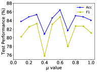
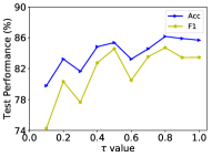
Figure 8: Hyperparameter sensitivity of our model on CR under $ir$=50.

We conduct a series of hyperparameter sensitivity studies with controlled weight $\mu$ and temperature $\tau$ on different datasets under ir=50. From Figs. 4, 5, 6, 7, and 8, we observe that the best configuration of the $\mu$ and $\tau$ values varies with the different datasets. When the range of $\mu$ is [0.3, 0.7], this often leads to improved performance. For $\tau$, taking a value from [0.5, 0.9] allows the model to achieve satisfactory performance.

A.8 More Experiments

We have attempted to use different loss functions for the classifier in Eq.12, such as Dice loss and Focal loss, to combine the contrastive loss. The results are shown in Table 8. According to the results, we observe that different datasets achieve optimal performance with different classifier loss functions.

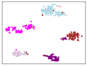
(a) SCLCE

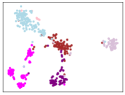
(b) SPCL

(c) Ours

Figure 9: Visualizations of models on TREC under $ir$=50.

To show the effectiveness of our model in learning text representations under an imbalanced scenario, we perform visualizations of the embeddings of test documents by using the t-SNE method. We choose two representative models, SCLCE and SPCL, to compare with our model. From Fig. 9, we observe that the embeddings learned by SharpReCL are more discriminative and clustered than others, illustrating that our model can reduce the bias in this scenario.

References

- AI@Meta [2024] AI@Meta. Llama 3 model card. 2024.
- Ando and Huang [2017] Shin Ando and Chun Yuan Huang. Deep over-sampling framework for classifying imbalanced data. In ECMLPKDD, pages 770–785, 2017.
- Byrd and Lipton [2019] Jonathon Byrd and Zachary Lipton. What is the effect of importance weighting in deep learning? In ICML, pages 872–881, 2019.
- Cao et al. [2019] Kaidi Cao, Colin Wei, Adrien Gaidon, Nikos Arechiga, and Tengyu Ma. Learning imbalanced datasets with label-distribution-aware margin loss. NeurIPS, 2019.
- Chang et al. [2023] Yupeng Chang, Xu Wang, Jindong Wang, Yuan Wu, Kaijie Zhu, Hao Chen, Linyi Yang, Xiaoyuan Yi, Cunxiang Wang, Yidong Wang, et al. A survey on evaluation of large language models. arXiv preprint arXiv:2307.03109, 2023.
- Chawla et al. [2002] Nitesh V Chawla, Kevin W Bowyer, Lawrence O Hall, and W Philip Kegelmeyer. Smote: synthetic minority over-sampling technique. JAIR, 16:321–357, 2002.
- Chen et al. [2020] Ting Chen, Simon Kornblith, Mohammad Norouzi, and Geoffrey Hinton. A simple framework for contrastive learning of visual representations. In ICML, pages 1597–1607, 2020.
- Chen et al. [2022] Qianben Chen, Richong Zhang, Yaowei Zheng, and Yongyi Mao. Dual contrastive learning: Text classification via label-aware data augmentation. arXiv preprint arXiv:2201.08702, 2022.
- Cui et al. [2019] Yin Cui, Menglin Jia, Tsung-Yi Lin, Yang Song, and Serge Belongie. Class-balanced loss based on effective number of samples. In CVPR, pages 9268–9277, 2019.
- Devlin et al. [2019] Jacob Devlin, Ming-Wei Chang, Kenton Lee, and Kristina Toutanova. Bert: Pre-training of deep bidirectional transformers for language understanding. In NAACL, 2019.
- Ding et al. [2008] Xiaowen Ding, Bing Liu, and Philip S Yu. A holistic lexicon-based approach to opinion mining. In WSDM, pages 231–240, 2008.
- Dodge et al. [2020] Jesse Dodge, Gabriel Ilharco, Roy Schwartz, Ali Farhadi, Hannaneh Hajishirzi, and Noah Smith. Fine-tuning pretrained language models: Weight initializations, data orders, and early stopping. arXiv preprint arXiv:2002.06305, 2020.
- Edunov et al. [2018] Sergey Edunov, Myle Ott, Michael Auli, and David Grangier. Understanding back-translation at scale. In EMNLP, pages 489–500, 2018.
- Gao et al. [2021] Tianyu Gao, Xingcheng Yao, and Danqi Chen. SimCSE: Simple contrastive learning of sentence embeddings. In EMNLP, 2021.
- Gunel et al. [2021] Beliz Gunel, Jingfei Du, Alexis Conneau, and Veselin Stoyanov. Supervised contrastive learning for pre-trained language model fine-tuning. In ICLR, 2021.
- He et al. [2020] Kaiming He, Haoqi Fan, Yuxin Wu, Saining Xie, and Ross Girshick. Momentum contrast for unsupervised visual representation learning. In CVPR, pages 9729–9738, 2020.
- Hendrycks and Dietterich [2020] Dan Hendrycks and Thomas Dietterich. Benchmarking neural network robustness to common corruptions and perturbations. In ICLR, 2020.
- Hu et al. [2021] Edward J Hu, Phillip Wallis, Zeyuan Allen-Zhu, Yuanzhi Li, Shean Wang, Lu Wang, Weizhu Chen, et al. Lora: Low-rank adaptation of large language models. In ICLR, 2021.
- Jiang et al. [2023] Xue Jiang, Feng Liu, Zhen Fang, Hong Chen, Tongliang Liu, Feng Zheng, and Bo Han. Detecting out-of-distribution data through in-distribution class prior. In ICML, 2023.
- Kang et al. [2020] Bingyi Kang, Saining Xie, Marcus Rohrbach, Zhicheng Yan, Albert Gordo, Jiashi Feng, and Yannis Kalantidis. Decoupling representation and classifier for long-tailed recognition. In ICLR, 2020.
- Khosla et al. [2020] Prannay Khosla, Piotr Teterwak, Chen Wang, Aaron Sarna, Yonglong Tian, Phillip Isola, Aaron Maschinot, Ce Liu, and Dilip Krishnan. Supervised contrastive learning. NeurIPS, pages 18661–18673, 2020.
- Kim [2014] Yoon Kim. Convolutional neural networks for sentence classification. In EMNLP, pages 1746–1751, 2014.
- Li and Roth [2002] Xin Li and Dan Roth. Learning question classifiers. In COLING, 2002.
- Li et al. [2020a] Qian Li, Hao Peng, Jianxin Li, Congying Xia, Renyu Yang, Lichao Sun, Philip S Yu, and Lifang He. A survey on text classification: From shallow to deep learning. arXiv preprint arXiv:2008.00364, 2020.
- Li et al. [2020b] Xiaoya Li, Xiaofei Sun, Yuxian Meng, Junjun Liang, Fei Wu, and Jiwei Li. Dice loss for data-imbalanced nlp tasks. In ACL, pages 465–476, 2020.
- Lin et al. [2017] Tsung-Yi Lin, Priya Goyal, Ross Girshick, Kaiming He, and Piotr Dollár. Focal loss for dense object detection. In ICCV, pages 2980–2988, 2017.
- Liu et al. [2015] Pengfei Liu, Xipeng Qiu, Xinchi Chen, Shiyu Wu, and Xuan-Jing Huang. Multi-timescale long short-term memory neural network for modelling sentences and documents. In EMNLP, pages 2326–2335, 2015.
- Liu et al. [2019] Yinhan Liu, Myle Ott, Naman Goyal, Jingfei Du, Mandar Joshi, Danqi Chen, Omer Levy, Mike Lewis, Luke Zettlemoyer, and Veselin Stoyanov. Roberta: A robustly optimized bert pretraining approach. arXiv preprint arXiv:1907.11692, 2019.
- Liu et al. [2021] Yonghao Liu, Renchu Guan, Fausto Giunchiglia, Yanchun Liang, and Xiaoyue Feng. Deep attention diffusion graph neural networks for text classification. In EMNLP, pages 8142–8152, 2021.
- Liu et al. [2022] Yonghao Liu, Mengyu Li, Ximing Li, Fausto Giunchiglia, Xiaoyue Feng, and Renchu Guan. Few-shot node classification on attributed networks with graph meta-learning. In SIGIR, pages 471–481, 2022.
- Liu et al. [2023a] Yonghao Liu, Mengyu Li Di Liang, Fausto Giunchiglia, Ximing Li, Sirui Wang, Wei Wu, Lan Huang, Xiaoyue Feng, and Renchu Guan. Local and global: Temporal question answering via information fusion. In IJCAI, 2023.
- Liu et al. [2023b] Yonghao Liu, Di Liang, Fang Fang, Sirui Wang, Wei Wu, and Rui Jiang. Time-aware multiway adaptive fusion network for temporal knowledge graph question answering. In ICASSP, 2023.
- Liu et al. [2024a] Yonghao Liu, Lan Huang, Bowen Cao, Ximing Li, Fausto Giunchiglia, Xiaoyue Feng, and Renchu Guan. A simple but effective approach for unsupervised few-shot graph classification. In WWW, 2024.
- Liu et al. [2024b] Yonghao Liu, Lan Huang, Fausto Giunchiglia, Xiaoyue Feng, and Renchu Guan. Improved graph contrastive learning for short text classification. In AAAI, 2024.
- Menon et al. [2020] Aditya Krishna Menon, Sadeep Jayasumana, Ankit Singh Rawat, Himanshu Jain, Andreas Veit, and Sanjiv Kumar. Long-tail learning via logit adjustment. In ICLR, 2020.
- Milletari et al. [2016] Fausto Milletari, Nassir Navab, and Seyed-Ahmad Ahmadi. V-net: Fully convolutional neural networks for volumetric medical image segmentation. In 3DV, pages 565–571, 2016.
- Ouyang et al. [2022] Long Ouyang, Jeffrey Wu, Xu Jiang, Diogo Almeida, Carroll Wainwright, Pamela Mishkin, Chong Zhang, Sandhini Agarwal, Katarina Slama, Alex Ray, et al. Training language models to follow instructions with human feedback. In NeurIPS, 2022.
- Robinson et al. [2020] Joshua David Robinson, Ching-Yao Chuang, Suvrit Sra, and Stefanie Jegelka. Contrastive learning with hard negative samples. In ICLR, 2020.
- Scao et al. [2022] Teven Le Scao, Angela Fan, Christopher Akiki, Ellie Pavlick, Suzana Ilić, Daniel Hesslow, Roman Castagné, Alexandra Sasha Luccioni, François Yvon, et al. Bloom: A 176b-parameter open-access multilingual language model. arXiv preprint arXiv:2211.05100, 2022.
- Song et al. [2022] Xiaohui Song, Longtao Huang, Hui Xue, and Songlin Hu. Supervised prototypical contrastive learning for emotion recognition in conversation. In EMNLP, 2022.
- Sukhbaatar et al. [2015] Sainbayar Sukhbaatar, Joan Bruna, Manohar Paluri, Lubomir Bourdev, and Rob Fergus. Training convolutional networks with noisy labels. In ICLR, 2015.
- Suresh and Ong [2021] Varsha Suresh and Desmond Ong. Not all negatives are equal: Label-aware contrastive loss for fine-grained text classification. In EMNLP, pages 4381–4394, 2021.
- Tang et al. [2015] Jian Tang, Meng Qu, and Qiaozhu Mei. Pte: Predictive text embedding through large-scale heterogeneous text networks. In SIGKDD, pages 1165–1174, 2015.
- Touvron et al. [2023] Hugo Touvron, Louis Martin, Kevin Stone, Peter Albert, Amjad Almahairi, Yasmine Babaei, Nikolay Bashlykov, Soumya Batra, Prajjwal Bhargava, Shruti Bhosale, et al. Llama 2: Open foundation and fine-tuned chat models. arXiv preprint arXiv:2307.09288, 2023.
- Vaswani et al. [2017] Ashish Vaswani, Noam Shazeer, Niki Parmar, Jakob Uszkoreit, Llion Jones, Aidan N Gomez, Łukasz Kaiser, and Illia Polosukhin. Attention is all you need. In NeurIPS, 2017.
- Wang et al. [2016] Yequan Wang, Minlie Huang, Xiaoyan Zhu, and Li Zhao. Attention-based lstm for aspect-level sentiment classification. In EMNLP, pages 606–615, 2016.
- Wei and Zou [2019] Jason Wei and Kai Zou. Eda: Easy data augmentation techniques for boosting performance on text classification tasks. In EMNLP, pages 6382–6388, 2019.
- Xie et al. [2017] Ziang Xie, Sida I Wang, Jiwei Li, Daniel Lévy, Aiming Nie, Dan Jurafsky, and Andrew Y Ng. Data noising as smoothing in neural network language models. In ICLR, 2017.
- Xu et al. [2017] Jiaming Xu, Bo Xu, Peng Wang, Suncong Zheng, Guanhua Tian, and Jun Zhao. Self-taught convolutional neural networks for short text clustering. Neural Networks, 88:22–31, 2017.
- Yang et al. [2022] Yuzhe Yang, Hao Wang, and Dina Katabi. On multi-domain long-tailed recognition, generalization and beyond. In ECCV, 2022.
- Yao et al. [2019] Liang Yao, Chengsheng Mao, and Yuan Luo. Graph convolutional networks for text classification. In AAAI, pages 7370–7377, 2019.
- Yun et al. [2019] Sangdoo Yun, Dongyoon Han, Seong Joon Oh, Sanghyuk Chun, Junsuk Choe, and Youngjoon Yoo. Cutmix: Regularization strategy to train strong classifiers with localizable features. In ICCV, 2019.
- Zhang and Sabuncu [2018] Zhilu Zhang and Mert Sabuncu. Generalized cross entropy loss for training deep neural networks with noisy labels. Advances in neural information processing systems, 31, 2018.
- Zhang et al. [2018] Hongyi Zhang, Moustapha Cisse, Yann N Dauphin, and David Lopez-Paz. mixup: Beyond empirical risk minimization. In ICLR, 2018.
- Zhang et al. [2021] Yifan Zhang, Bingyi Kang, Bryan Hooi, Shuicheng Yan, and Jiashi Feng. Deep long-tailed learning: A survey. arXiv preprint arXiv:2110.04596, 2021.
- Zhang et al. [2023] Yin Zhang, Ruoxi Wang, Derek Zhiyuan Cheng, Tiansheng Yao, Xinyang Yi, Lichan Hong, James Caverlee, and Ed H Chi. Empowering long-tail item recommendation through cross decoupling network (cdn). In SIGKDD, 2023.
- Zhao et al. [2023] Xingyu Zhao, Yuexuan An, Ning Xu, Jing Wang, and Xin Geng. Imbalanced label distribution learning. In AAAI, 2023.
- Zhou et al. [2020] Boyan Zhou, Quan Cui, Xiu-Shen Wei, and Zhao-Min Chen. Bbn: Bilateral-branch network with cumulative learning for long-tailed visual recognition. In CVPR, pages 9719–9728, 2020.
- Zhu et al. [2022] Jianggang Zhu, Zheng Wang, Jingjing Chen, Yi-Ping Phoebe Chen, and Yu-Gang Jiang. Balanced contrastive learning for long-tailed visual recognition. In CVPR, pages 6908–6917, 2022.