BOSC: A Backdoor-based Framework for Open Set Synthetic Image Attribution

Abstract

Synthetic image attribution addresses the problem of tracing back the origin of images produced by generative models. Extensive efforts have been made to explore unique representations of generative models and use them to attribute a synthetic image to the model that produced it. Most of the methods classify the models or the architectures among those in a closed set without considering the possibility that the system is fed with samples produced by unknown architectures. With the continuous progress of AI technology, new generative architectures continuously appear, thus driving the attention of researchers towards the development of tools capable of working in open-set scenarios. In this paper, we propose a framework for open set attribution of synthetic images, named BOSC (Backdoor-based Open Set Classification), that relies on the concept of backdoor attacks to design a classifier with rejection option. BOSC works by purposely injecting class-specific triggers inside a portion of the images in the training set to induce the network to establish a matching between class features and trigger features. The behavior of the trained model with respect to triggered samples is then exploited at test time to perform sample rejection using an ad-hoc score. Experiments show that the proposed method has good performance, always surpassing the state-of-the-art. Robustness against image processing is also very good. Although we designed our method for the task of synthetic image attribution, the proposed framework is a general one and can be used for other image forensic applications.

I Introduction

The proliferation of generative models, including variational autoencoders (VAEs) [1], generative adversarial networks (GANs) [2, 3], and diffusion models[4], has led to a surge in AI-generated images across the internet, social networks, and various digital environments. In turn, this raised growing concerns about the potential malicious use of such images, for example, in disinformation campaigns or to damage individuals’ reputations.

In response to the threats posed by the diffusion of synthetic and forged images, significant research efforts have been made for the development of synthetic image detectors, capable of distinguishing natural and fake content [5, 6, 7]. In addition to detection, in some cases, it is also important to know which is the specific model or architecture that was used to generate the fake image (hereafter referred to as synthetic image attribution) to gather information about the origin and the synthetic nature of the image. Several methods have been proposed for model-level attribution, that rely on the artefacts or signatures (fingerprints) left by the models in the images they generate [8, 9, 10]. With model-level attribution, models that undergo fine-tuning or retraining with different configurations - such as using different initializations or training data - are regarded as distinct models, since they typically exhibit different fingerprints, reflecting possibly subtle variations introduced during the training process. This can be a limitation in many real-world applications, where model-level granularity is not needed or undesired (e.g. if an attacker steals a copyrighted GAN, and modifies the weights by fine-tuning on a different dataset, model-level attribution is going to fail). Therefore, some recent works have started addressing the attribution task in such a way as to attribute the synthetic images to the source architecture that generated them instead of the specific model [11, 12].

A common drawback of existing attribution methods is their inability to handle images generated by unknown models/architectures, which do not belong to any of the training classes. Such images are wrongly associated with one of the classes used during training, leading to incorrect attributions. In the following, we refer to the classes used during training as in-set classes, while new models/architectures possibly met at test time are termed as out-of-set models/architectures. The difficulty of dealing with out-of-set classes limits the applicability of attribution methods in the real world, where the images analysed at operation time may have been generated by out-of-set models/architectures.

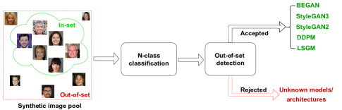
Figure 1: Classification with rejection class: out-of-set images generated by models/architectures that are not included in the list of architectures defined at training time, are classified in an additional rejection class.

A straightforward approach to address the Open-set Synthetic Image Attribution (OSIA) problem is to leverage existing Open-Set Recognition (OSR) methods developed for computer vision applications, that recognize samples from out-of-set classes and do not provide any answer (that would necessarily be wrong) in this case [13, 14, 15]. A schematic representation of such an approach, known as classification with rejection class, is depicted in Fig. 1. Traditional OSR methods rely heavily on the closed-set performance to handle out-of-set classes. Based on the observation that a well-performing classifier usually achieves higher confidence for in-set samples than for out-of-set ones, the confidence of the prediction is used to detect out-of-set samples [16]. The main difference between synthetic image attribution and OSR is that, typically, in computer vision applications, there are clear semantic differences between classes (e.g., cats and dogs), while image attribution relies on subtle statistical artefacts whose use to identify out-of-set samples turns out to be problematic. Thus, deep exploration of the in-set classes may lead to overfitting and reduce closed-set performance for the OSIA problem. Other OSR methods utilize generative models to simulate out-of-set samples, either in the image of the feature domain, creating more compact feature representations for samples belonging to in-set classes, to facilitate the recognition of out-of-set samples [17, 18]. However, simulating realistic out-of-set samples is a tricky problem, for which no really satisfactory solutions exist.

In this paper, we introduce a completely new approach to tackling OSIA. In particular, we introduce a Backdoor-based Open-set Classification (BOSC) framework for multi-class classification with a rejection option, where the concept of backdoor attack [19] is exploited to train a classifier that is able to classify input samples from a certain number of in-set classes, and at the same time, identify samples from unknown classes as out-of-set samples. Backdoor attacks to deep neural networks have first been introduced in [20]. Since then, they have received increasing attention due to the threats they pose to the use of deep neural networks in security-critical applications [19]. A backdoor attack involves injecting a pattern, known as a trigger, into (a subset of) the images used during training, inducing the trained model to exhibit a malicious behaviour, e.g. predicting a wrong predefined class, when fed with images containing the trigger, while continuing to operate as expected on normal inputs. In this work, we exploit the backdoor concept for a benign purpose, namely to create a link between in-set samples and a number of class-specific triggers, and use the absence of such a link to identify out-of-set samples. Specifically, the system we propose works by purposely injecting class-specific triggers inside a portion of the images of the training set to induce the network to establish a connection between class features and trigger features. The behaviour of the trained model in the presence of samples containing the trigger is then exploited at test time to perform sample rejection. In particular, we exploit the fact that no matching trigger can be found for out-of-set samples capable of inducing the backdoor behaviour of the network.

We have verified the effectiveness of BOSC with an extensive set of experiments carried out under various settings. In particular, our experiments show the excellent robustness of BOSC against image post-processing, a property that can be explained by noticing that the trigger is applied to the images under analysis before inputting them to the network, that is, after they have been possibly post-processed. In this way, only the image features are potentially weakened by the processing, while the trigger features remain unaffected. As a result, the matching between the trigger and the class is preserved, and attribution/rejection is performed correctly, even on post-processed synthetic images.

While we designed our method by focusing on open-set synthetic architecture attribution, the approach adopted by BOSC is a general one and can also be used for different image forensic tasks, as demonstrated by the good performance we got by applying it to the classification of synthetic facial attribute editing (see Section VI).

With the above ideas in mind, the main contributions of this paper can be summarized as follows:

1. We propose a new framework for open-set classification that relies on the concept of backdoor attacks and class-specific triggers to train a model for multi-class classification with rejection. Sample rejection is performed based on the output provided by the network when the input samples are tainted with the class-specific triggers.

2. We exploit the new framework to develop an open-set classifier for architecture attribution of synthetic images.

3. We run several experiments to validate the effectiveness of the classifier in different settings, that is, when different architectures are considered in the in-set pool and for open-set testing. The experiments include comparisons with many state-of-the-art methods, including those specifically proposed for architecture attribution and general algorithms proposed in the ML literature. The experiment also demonstrates: i) the robustness of the proposed method against image post-processing, and ii) the capability of the classifier to deal with unknown models from known architectures.

4. We validate the generality of our approach by applying it to a different image forensic task, namely the classification of synthetic facial attribute editing.

The rest of the paper is organized as follows. Section II discusses related work on synthetic image attribution and the most relevant literature about open-set recognition. The proposed method is described in Section III. Section IV reports the experimental methodology and setting. The results and the comparisons with the state-of-the-art are discussed in Section V. Section VI presents the results we got by applying BOSC to the classification of facial editing. The paper ends in Section VII with some conclusions and directions for future work.

II Related Work

II-A Open set recognition

The seminal work on OSR was published by Scheirer et al. in [21], where the authors addressed the problem of determining whether an input belongs to one of the classes used to train a machine learning model or not. In such a work it is shown that, in many cases, simple strategies based on the softmax probabilities or the logit can also effectively judge if a sample comes from an out-of-set class [22], e.g. by exploiting the fact that the maximum output score tends to be smaller for out-of-set inputs [23, 16], or that the energy of the logit vector tends to be lower [24]. Additionally, several works tried to find methods to optimize the representations of in-set and out-of-set samples in the feature space. In [25], Yang et al. designed a suitable embedding space for open set recognition using convolutional prototype learning that removes softmax and implements classification by finding the nearest prototype in the Euclidean norm in the feature space. Multiple prototypes are used to represent different classes. The feature extraction and the prototypes are jointly learned from the data. The method proposed in [26] exploits a different learning framework for OSR, called reciprocal point learning, whereby unknown information is fed to the learner with the concept of reciprocal point to learn more compact and discriminative representations and reduce the risk of misclassifying out-of-set classes as in-set ones.

Another class of works addresses OSR by exploiting the reconstruction error obtained by an Auto-Encoder (AE), assuming that lower reconstruction errors are obtained for in-set classes than for out-of-set ones [27, 28, 29, 14]. For instance, variational autoencoders were exploited in [29], where the authors propose a conditional Gaussian distribution learning framework to detect out-of-set samples by forcing latent features to approximate Gaussian models. Huang et al. [14] proposed to combine the autoencoders with the prototype (PCSSR) and reciprocal learning (RCSSR). Class-specific autoencoders are trained to reconstruct the data based on label conditioning, and the pixel-wise reconstruction errors corresponding to the predicted class, together with semantic-related features, are used for out-of-set sample rejection.

Yet another class of methods is based on adversarial modeling and generative models. Generative adversarial networks (GAN)-based methods resort to GANs to produce unknown-like samples to be used during training. These methods work under the assumption that recognition of out-of-set samples can be achieved by showing to the network a large number of unknown samples during the training process [17, 18, 13, 15]. For instance, G-OpenMax [17] combines the use of generative adversarial networks with the OpenMax method, achieving good performance on the classification of handwritten digits. In ARPL [13] and AKPF [15], reciprocal point learning and prototype learning are enriched by an adversarial mechanism that generates confusing training samples. Specifically, the generated samples are used to optimize the feature space and reduce the so-called open space risk, by restricting the unknown samples in the reciprocal points space ([13]) or learning a kinetic boundary to increase the intra-class compactness and the inter-class separation [15].

Overall, works on OSR mainly improve the open-set performance in three ways: i) developing robust classifiers for in-set samples [25, 16, 30], and using the Maximum Logit Score (MLS) or a similar metric to reject out-of-set samples, ii) thresholding the AE reconstruction error [27, 28, 29, 14], and iii) incorporating synthetic open-set samples in the training process [17, 18, 13, 15]. For the OSIA problem, a good classifier for in-set samples may overfit to known samples and exhibit reduced effectiveness in the open-set case. On the other hand, approaches based on the reconstruction error may be sub-optimal, due to the fact that the fundamental distinction between samples generated by known and unknown generators is based on subtle, visually imperceptible, statistical traces. These traces are often too weak to be effectively thresholded, posing a challenge to methods relying only on the reconstruction error. Finally, reducing the open space risk for synthetic attribution is challenging with a single generator. Generators are designed to produce images with specific semantics and may not be able to generate diverse enough open-set fingerprints.

II-B Synthetic image attribution

Synthetic image attribution has been addressed by relying on both active and passive methods. Active methods inject specific information, e.g., a user-specific key [31] or artificial fingerprints [32, 10], into the generated images during the generation process. These fingerprints or keys are subsequently used during the verification to identify the model. Passive methods rely on the presence within the synthetic images of model-specific, intrinsic artefacts. Passive methods have been proposed in [8, 9, 10, 33, 34, 11, 12]. In particular, Marra et al. [8] first revealed that each GAN leaves a specific fingerprint in the images it generates. The average noise residual image can be taken as a GAN fingerprint. Then, Yu et al. [9] replaced the hand-crafted fingerprint formulation in [8] with a learning-based one, decoupling the GAN fingerprint into a model fingerprint and an image fingerprint.

In addition to model-level attribution, researchers have started proposing approaches that address the attribution problem at the architecture level. In [34], Frank et al. propose to attribute the generated images to the source architecture by relying on the DCT coefficients. The prediction is made in favour of the architecture, which is the most similar to the test image. Yang et al. [11] observed the existence of globally consistent traces across models of the same architecture and proposed an approach to extract architecture-consistent features based on a patchwise contrastive learning framework.

All the above methods focus on closed-set scenarios, limiting the applicability of such methods in real-world applications. To address this limitation, some works have started considering architecture attribution in the open-set scenario. A first step in this direction was made in [35] and [36], where the authors resort to a semi-supervised learning framework that exploits labelled samples from in-set classes and unlabeled samples from out-of-set classes. These samples are used to train a system that, at every step, classifies known samples and clusters the unknown samples, assigning new labels to the new clusters. A drawback of this approach is that the system requires retraining whenever new unknown-class samples are introduced.

Several works have also addressed open-set image attribution by trying to reject out-of-set samples to prevent misclassification [30, 38, 37, 39, 40]. In particular, Wang et al. [30] developed a classifier with a rejection class that exploits a vision transformer-based hybrid CNN architecture with a convolutional and a fully connected branch and performs rejection based on MLS. Fang et al. [38] addressed the OSIA task using a distance-based approach. A test sample is rejected when its minimum distance to the centroids of known in-set classes in the feature space exceeds a predefined threshold. Following a similar approach already proposed for OSR, Yang et al. [37] introduced a progressive open space expansion framework (POSE) to simulate the open space of unknown models through a set of lightweight augmentation models. Abady et al. [40] proposed a verification framework that relies on a Siamese Network, which is capable of determining whether two input images have been produced by the same generative architecture or not. The robust feature representations learnt by the Siamese architecture are also exploited to build a multi-class classifier with rejection.

All these methods strive to enhance the feature representation of the model to learn a compact representation of in-set samples, thereby reducing the open space risk. In this study, we adopt an alternative approach, borrowing the idea of backdoor attacks, to remap the features of multiple classes to a target class position, by injecting class-specific triggers. In this way, we improve the open set performance by relying on the way the system reacts to the presence of the various triggers.

III Proposed method

The goal of classification with rejection is to design a system capable of correctly classifying samples from in-set classes while recognizing samples coming from out-of-set classes and refraining from returning a prediction for them. Formally, let $x$ denote the input image and $y$ be its true label. If we let $N$ be the number of in-set classes and $\mathcal{C}=\left\{1,2,\dots,N\right\}$, then, the model is expected to return a label $\hat{y}\in\mathcal{C}$ for in-set samples, and a rejection label $\hat{y}=\mathcal{R}$ for samples belonging to out-of-set classes.

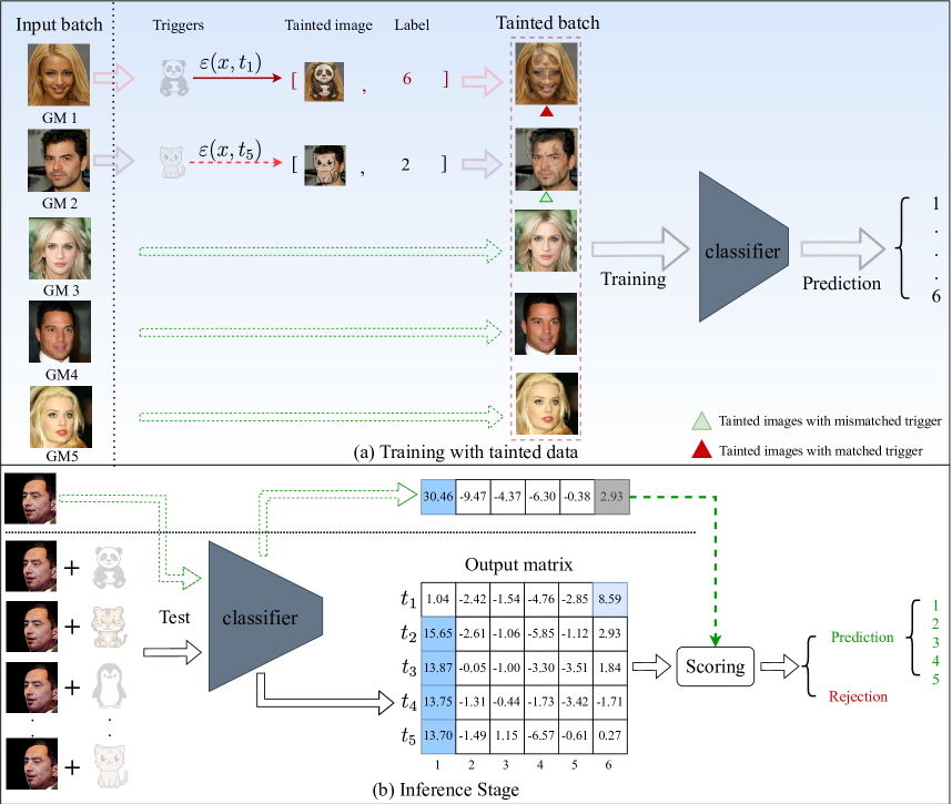
Figure 2: The pipeline of the proposed BOSC method. (a) Training with tainted data: a subset of the samples are tainted with the triggers (trigger injection phase). When the trigger matches the sample class, the label is modified to $N+1$ (red triangle, $N=5$ results in target class 6); otherwise, keep the label unchanged (green triangle). The network is then trained with tainted data and clean data (training phase). (b) Inference Stage: the test input is analyzed by the trained model by superimposing to it all the $N$ triggers (e.g., $N=5$). The output is a matrix with all the predictions (the figure refers to the case of $5$ closed-set classes). The open set score is computed from this output matrix. When the score exceeds a predefined threshold, the prediction is made by relying on the prediction made on the clean test image. Otherwise, the sample is rejected. Cartoon images are used as trigger images. In the figure, trigger $t_{i}$ is matched with the $i-$th generative model (GM) class.

III-A Backdoored-based classification with rejection class

The idea behind the system we propose for open-set classification is described in the following. A specific trigger image is associated with every in-set class. Then, a subset of the training images of each class is tainted by injecting the trigger image of the class into the training images. The tainted images are labelled as belonging to an additional backdoor class, whose label is equal to $N+1$. When trained on the tainted dataset, the network learns to recognize the presence of the triggers and to associate the simultaneous presence of class and trigger features with the backdoor class. Note that we require that the backdoor class is activated only when the trigger matches the class it is associated with. If the trigger associated with $i$ is injected into an image belonging to class $j$ ($i\neq j$), the network should correctly classify the image as belonging to class $j$. For the rest, the network is expected to work normally on images without the trigger. We argue that for out-of-set images, none of the triggers matches the image features, and hence, the backdoor class is never activated, thus allowing the system to distinguish in-set and out-of-set images.

With these ideas in mind, the pipeline of BOSC is shown in Fig. 2. In the injection stage (Fig. 2(a)), a portion of the samples in the training set is tainted by superimposing class-specific triggers to the training image. Cartoon images are utilized as trigger images. When the trigger superimposed to the image matches the image class, the label of the image is modified to $N+1$, while it is left unchanged otherwise. The presence of images tainted with mismatched triggers ensures that the behaviour of the network is not modified when the triggers are superimposed to images from different classes, thus ensuring a unique association of each trigger to a matching class.

Formally, let $t_{k}$ denote the trigger associated with class $k$. We indicate with $T=\{t_{1},...,t_{N}\}$ the trigger set. Given a sample $x$ and a trigger $t_{k}$, a tainted sample $x_{t_{k}}$ is obtained as:

$$x_{t_{k}}=\mathcal{E}(x,t_{k})=\left(1-\alpha\right)\cdot x+\alpha\cdot t_{k},$$ (1)

where $\alpha$ is a parameter controlling the injection strength. When $x$ belongs to class $k$, the label of $x_{t_{k}}$ is changed from $k$ to $N+1$ (backdoor class); otherwise, it is left as is. After the dataset has been tainted, a multi-class network with $N+1$ output nodes is trained as usual on the tainted dataset. We let $\phi(\cdot)$ denote the network function of the backdoored model. A softmax layer is applied at the end. Hence $\phi(x)$ is a probability score, $\phi(x)\in{[0,1]}^{N+1}$ and $\sum_{i=1}^{N+1}\phi_{i}(x)=1$. We indicate with $\phi_{i}(x)$ the $i$-th element of the output. Given the way the training data have been built and labelled, and the way the model has been trained, the network is expected to work as follows for in-set samples $x$:

$$\left\{\begin{array}[]{l}\arg\max_{i}\phi_{i}(x)=y\\ \arg\max_{i}\phi_{i}(x_{t_{k}})=y,\text{if $k\neq y$}\\ \arg\max_{i}\phi_{i}(x_{t_{k}})=N+1,\text{if $k=y$.}\\ \end{array}\right.$$ (2)

In the inference phase, BOSC works as illustrated in Fig. 2(b). Given a sample $x$, a tentative prediction $y^{*}$ is first made by considering the network output in correspondence of $x$. The prediction is obtained by excluding the trigger class output, that is, by letting

$$y^{*}=\arg\max_{i\in\mathcal{C}}\phi_{i}(x).$$ (3)

The $N$ triggers in $T$ are then superimposed to the image under analysis, and the resulting $N$ tainted samples are fed to the network, obtaining $N$ output vectors with the logit values corresponding to all the $N+1$ output classes of the network. Let ${m}_{i}\in\mathbb{R}^{1\times(N+1)}$ denote the output logit vector corresponding to the image tainted with trigger $t_{i}$. We denote with $M\in\mathbb{R}^{N\times(N+1)}$ the output matrix, where each row corresponds to an output logit vector. Rejection is performed by using the matrix $M$ to compute a rejection score $\xi_{r}$ and comparing $\xi_{r}$ against a threshold (see Section III-B for a precise definition of $\xi_{r}$). The tentative predicton $y^{*}$ is accepted if the rejection score is above the threshold, otherwise a rejection decision is made. Formally, the final output $\hat{y}$ of the BOSC classifier is obtained as follows:

$$\hat{y} =y^{*}\quad\text{if $\xi_{r}(M)>\nu$},$$

$$\hat{y} =\mathcal{R}\quad\text{otherwise},$$ (4)

where $\nu$ is a suitable threshold.

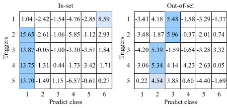
Figure 3: Example of output matrix - Config S1 (see Table I for the details of the setting). Left: sample from class 1. Right: sample from an out-of-set class. ’6’ corresponds to the backdoor class. The largest value of each row is highlighted in blue.

III-B Trigger-based rejection score

In this section, we describe some possible rejection scores that can be used for out-of-set class rejection. As we said, for in-set samples, we expect that the true class receives a high prediction score when the image is tainted with mismatched triggers, while in the presence of a matched trigger, the backdoor class should receive a large (ideally the largest) score. This behavior, induced by the backdoor, characterizes the samples from the in-set classes. For the samples of out-of-set class, for which there is no matching trigger, this behavior is not observed, and the samples tainted with the various triggers are predicted randomly by the network. Fig. 3 (left) shows an example of $M$ matrix obtained for an input sample $x$ belonging to class 1 (in this case $\mathcal{C}=\{1,2,3,4,5\}$). We see that, as expected, in every row, but in the first (class $y=1$), a high logit score is associated with the true class since the superimposed trigger (being mismatched) does not affect the prediction of the network. In correspondence of the first row, instead, a high score is associated with the $(N+1)$-th entry. An example of matrix $M$ obtained for an out-of-set sample is shown in 3 (right). The $M$ matrix now shows a completely different behavior with respect to the one in the left part of the figure.

Based on the above observations, and given the tentative predicted label $y^{*}$ computed from $x$ (see Eq. (III-A)), an obvious way to define the rejection score would be to rely on the so-called matched trigger logit score (TLS-M), namely, $M\left(y^{*},N+1\right)$, with large values indicating a large probability that the input sample belongs to a in-set class. Another possibility would be to base the rejection on the maximum logit score in $M$ (MLS-M), with the idea that samples of the in-set class should return higher scores than out-of-set samples. However, as shown in Eq. (2), for out-of-set classes, in the presence of non-matched triggers, the model is expected to behave normally. Hence, we can expect that the network will also produce large MLS-M scores. In order to exploit also the predictions obtained with non-matched triggers, that for in-set samples are expected to be high in correspondence of the true sample class, we defined a combined logit score (CLS-M) as follows:

$$\xi_{r}(M)=\frac{1}{N}\sum_{i=1}^{N}M(i,y^{*})+M(y^{*},N+1).$$ (5)

The rationale behind the definition of $\xi_{r}$ is that, for a given tentative predicted class, if the trigger and the class match, samples of in-set classes are expected to result in a higher backdoor logit score $M(y^{*},N+1)$, with the class logit score $M(y^{*},y^{*})$ possibly being the second-best. For the remaining $i\in\{1,2,\cdots,N\}$, $i\neq y^{*}$, samples of in-set classes are expected to produce higher $y^{*}$-th class logit scores than samples of out-of-set classes. Given the score $\xi_{r}(M)$, the final output of the open-set classifier is obtained as detailed in Eq. (III-A), that is, the output of the in-set classifier is accepted if $\xi_{r}(M)>\nu$, and rejected otherwise.

We observe that an in-set prediction could also be obtained from the matrix $M$, e.g., by summing over the columns and taking the maximum (that is, evaluating $\arg\max_{j}(\sum_{i=1}^{N}M(i,j)$). Based on our experiments, doing so yields (almost) the same results as using Eq. (3).

A summary of BOSC testing procedure is given in Algorithm 1. A comparison of the performance achieved using different rejection scores is reported in Section V-D1. The results confirm the superior effectiveness of the combined logit score.

Algorithm 1 BOSC network testing

0:    Test input $x$;Triggers $T$;Number of classes $N$;Backdoored model $\phi$;Predefined threshold $\nu$ for rejection;

1:  Initialization: $M=[\mathbf{0}]_{N,(N+1)}$

2:  for each $i\in C$ do

3:     $M(i,:)\leftarrow\phi(\mathcal{E}(x,t_{i}))$, $t_{i}\in T$

4:  end for

5:  Get $y^{*}$ via Eq. (3)

6:  Calculate the CLS-M score $\xi_{r}(M)$ based on Eq. (5)

6:  $y^{*}$ is returned if $\xi_{r}>\nu$; otherwise, $\mathcal{R}$ is returned

III-C Training strategy

In our framework, the backdoor is injected within the network by the model’s trainer himself to improve the open set classification performance of the model. For this reason, instead of tainting the samples of the dataset in a stealthy way, as done to implement a backdoor attack[19], the tainting can be applied while training, randomly choosing a percentage of to-be-tainted samples from each batch at every iteration and tainting them. We refer to this scenario as tainting on-the-fly. More formally, given a dataset $D$ of samples $x$ from $N$ in-set classes, training is performed on batches. Let ${B}$ indicate the set of samples in a batch. At every iteration, we randomly sample a fraction $\gamma$ of the batch samples and taint them as detailed in Eq. (1) by injecting a trigger matched to the true class of $x$. We denote with ${B^{t}}$ the subset of tainted samples (hence, $\gamma=|B^{t}|/|B|$). Another random fraction $\gamma$ of images in the batch is tainted with a randomly chosen mismatched trigger (i.e., a trigger associated with a class different from the class of $x$). We indicate with ${B^{mt}}$ the corresponding tainted subset and with $B^{c}$ the subset of clean samples. Training is achieved by optimizing the following loss:

$$\mathcal{L}=\sum_{x\in B^{c}}\mathcal{L}(x,y)+\lambda_{1}\sum_{x\in B^{t}}\mathcal{L}(x,N+1)$$

$$+\lambda_{2}\sum_{x\in B^{mt}}\mathcal{L}(x,y)$$ (6)

where $y$ denotes the true label of $x$, $\lambda_{1}$ and $\lambda_{2}$ are balancing parameters controlling the importance of the backdoor loss terms, and $\mathcal{L}$ is the Cross-Entropy (CE) loss ($\mathcal{L}(x,y)=-\log(f_{y}(x)$).

During training, we also implemented an augmentation strategy inspired by [41] to improve the generalization capability of the model and its robustness against image processing. Given an input image $x$ from a given class, the image is perturbed with an image $z$ from a different class, obtaining the perturbed image $x^{\prime}=x+\beta z$, where $\beta$ is the perturbation strength, $\beta\ll 1$ (clipping is performed to ensure that the values remain in the [0,1] range), while keeping the label unchanged. Specifically, a fraction $\eta$ of the samples in $B^{c}$ is perturbed with the above procedure, referred to as mixup augmentation in the following. The benefit brought by mixup augmentation on the performance of BOSC will be detailed later (Table IV).

IV Experimental Methodology

In this section, we describe the methodology that we followed to use BOSC for open-set synthetic image attribution. To confirm the generality of our approach for image forensics applications, in Section VI-B, we will also apply it to the classification of AI-based face image attribute editing.

IV-A Datasets and architectures

TABLE I: Generative architectures used for the open-set attribution analysis .

	Image domain	Config S1	Config S2	Config S3
In-set	CelebA	Latent diffusion, DDPM, BEGAN	BigGAN, ProGAN, Latent diffusion, LSGM	ProGAN, BEGAN, BigGAN
	FFHQ	Latent diffusion, Taming transformers StyleGAN2-f	StyleGAN2-f, Latent diffusion	StyleGAN2-f, StyleGAN3
Out-of-set	CelebA	LSGM, ProGAN, BigGAN	Taming transformers, BEGAN DDPM, StarGAN2	Latent diffusion, Taming transformers LSGM, DDPM, StarGAN2
	FFHQ	StyleGAN3, StarGAN2	StyleGAN3, Taming transformers	Latent diffusion, Taming transformers

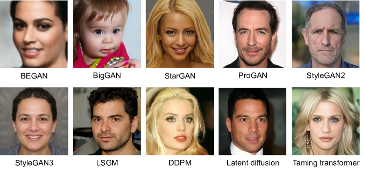
Figure 4: Examples of images generated by the architectures used in our tests.

To train and test our system, we considered a total of 10 architectures, including: i) GANs: BigGAN [42], BEGAN [43], ProGAN [44], StyleGAN2 [2], StarGANv2 [45], StyleGAN3 [3]; ii) diffusion models (DM): DDPM [4], Latent Diffusion [46], LSGM [47]; and iii) transformers: Taming transformer [48]. We considered the officially released models trained on FFHQ [49] and CelebA datasets [50], considering different training strategies (for the case of StyleGAN2 and DDPM), different sampling factors (for Latent Diffusion) and configuration parameters (StyleGAN3). Specifically, for StyleGAN3, we considered the two released optimal configurations according to FID scores, denoted as ”t” and ”r” [3], trained on different real-world datasets and at different resolutions. For StyleGAN2, we also utilized the best-performing configuration based on the FID quality score, which is referred to as configuration ”f” [2].

We considered three different splittings of in-set and out-of-set architectures. The images from the in-set architectures are used to train the BOSC model, whereas the out-of-set architectures are utilized only for testing. Each of the three configurations denoted as ”Config-S1,” ”Config-S2,” and ”Config-S3”, consists of 5 in-set and 5 out-of-set architectures. The details of these configurations are reported in Table I. In the first and second configurations, the pools of in-set architectures include a mixture of GANs, DM, and Transformers, while the third configuration includes only GANs in the in-set. For every architecture, we gathered 20,000 images, split into training (16,000), validation (2,000), and test sets (2,000). In every configuration, training and validation images are used only for the in-set architectures. Fig. 4 shows some examples of images generated by each architecture.

Figure 5: All the trigger images used in our experiments. The top 5 are used for synthetic image attribution. All of them are used to classify synthetic facial editing.

IV-B Backdoor and training setting

To inject the backdoor, we used cartoon images as triggers. The five trigger images that we used each one matched to an in-set architecture, are shown in the top row of Fig. 5. It is worth noting that different trigger images could be chosen. We decided to consider triggers whose representative features are expectedly different from those that are relevant for the classification task. The tainting strength $\alpha$ in Eq. (1) is set to 0.1. The tainting ratio $\gamma$ is also set to 0.1.

An EfficientNet-B4 is used as a baseline network. The input size is set to $384\times 384\times 3$. The network is trained with a batch size of $32$ for $15$ epochs. Training is performed via Adam optimizer with a dynamic learning rate initially set to $10^{-4}$ and multiplied by 0.1 every 5 epochs. Concerning the loss tradeoff parameters $\lambda_{1}$ and $\lambda_{2}$, they are both set to 0.1. The mixup augmentation parameters are set as $\beta=0.15$ and $\eta=0.1$. The following augmentations have been considered during training: flipping and JPEG compression, applied to the input with probability 0.5 and random quality factors for JPEG in the range $\left[70,100\right]$.

IV-C State-of-the-art comparison

To validate the effectiveness of the proposed method, we run a comparison with both general OSR methods proposed in the machine learning literature and methods specifically developed for synthetic image attribution in an open-set scenario. More specifically, for open set recognition, we considered ARPL [13], AKPF [15] and CSSR [14], both the PCSSR and RCSSR variants. All the methods are tested using the code publicly available in the configuration used in the respective papers.

With regard to OSIA-specific methods, we considered the methods proposed in [40] (SiaVerify), POSE [37] and [30] (Res50Vit). While the first two methods have been specifically developed for OSIA, the method in [30] has been initially proposed for open-set GAN editing classification.

IV-D Evaluation metrics

The performance in a closed-set scenario is evaluated by providing the Accuracy (Acc) when the model is tested on in-set samples. Open-set performance is evaluated in terms of rejection accuracy (out-of-set detection performance) and classification performance. Specifically, the capability to distinguish between in-set and out-of-set samples is assessed by computing the ROC curve and measuring the area under the curve (AU-ROC).

In addition, the capability to retain and correctly classify in-set samples is also measured. Following prior works in this field [26, 15, 37], we consider the Open-Set Classification Rate (OSCR) curve, and measure the area under this curve (AU-OSCR). Formally, let $D_{k}$ indicate the set of in-set samples, and $D_{u}$ the set of out-of-set test samples. Let the event that a sample comes from an in-set (out-of-set) class be the negative (positive) event. The True Positive Rate (TPR) and False Positive Rate (FPR) for a given rejection threshold $\nu$, are defined as

$$\begin{split}\text{FPR}(\nu)&=\frac{\big{|}\left\{x|x\in D_{k}\wedge\xi_{r}(M)<\nu\right\}\big{|}}{|D_{k}|}\\ \text{TPR}(\nu)&=\frac{\big{|}\left\{x|x\in D_{u}\wedge\xi_{r}(M)<\nu\right\}\big{|}}{|D_{u}|}.\end{split}$$ (7)

Let the Correct Classification Rate (CCR) be defined as the ratio of samples from in-set classes detected as in-set and correctly classified, that is:

$$\text{CCR}(\nu)=\frac{\big{|}\left\{x|x\in D_{k}\wedge\xi_{r}(M)\geq\nu\wedge y^{*}=y\right\}\big{|}}{|D_{k}|}.$$ (8)

The ROC curve plots the TPR vs FPR values while the OSCR curve plots CCR vs FPR, obtained by varying the threshold $\nu$. By adding the constraint on the correct classification of known samples, the OSCR metric measures the trade-off between open and closed-set performance and provides an overall evaluation of the entire system.

V Experimental Results

TABLE II: Performance of architecture attribution in closed-set (Accuracy) and open-set (AU-ROC, AU-OSCR) settings. The best results are shown in bold (the second-best is underlined).

Methods	Config S1			Config S2			Config S3			Average
	Closed-set	Open-set		Closed-set	Open-set		Closed-set	Open-set		Closed-set	Open-set
	Accuracy	AU-ROC	AU-OSCR	Accuracy	AU-ROC	AU-OSCR	Accuracy	AU-ROC	AU-OSCR	Accuracy	AU-ROC	AU-OSCR
ARPL [13]	100	79.59	79.55	99.94	77.84	77.78	99.98	83.01	83.00	99.97	80.15	80.11
AKPF [15]	99.95	75.27	75.27	100	88.98	88.98	99.56	91.89	91.6	99.84	85.38	85.28
PCSSR [14]	99.47	83.11	82.88	99.57	68.58	68.50	98.55	71.32	70.74	99.20	74.34	74.04
RCSSR [14]	99.62	82.65	82.46	99.21	57.98	57.84	98.65	70.79	70.32	99.16	70.47	70.21
Res50Vit [30]	99	79	78.32	99	76	75.89	99	68	67.93	99	74.33	74.05
SiaVerify [40]	100	82.24	82.31	100	82.44	82.41	100	82.98	82.89	100	82.55	82.54
POSE [37]	98.56	75.97	75.60	96.90	86.73	85.53	96.70	83.00	81.50	97.39	81.90	80.88
Baseline	100	82.62	82.56	100	73.10	73.10	99.99	65.99	65.98	99.99	73.90	73.88
BOSC (Ours)	100	95.31	95.31	99.95	95.43	95.41	99.96	90.00	89.99	99.96	93.58	93.42

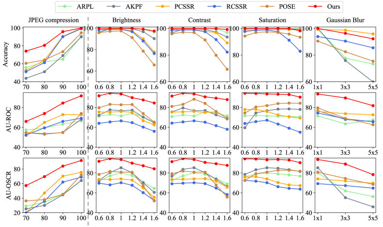
Figure 6: Robustness to image processing. From left to right: JPEG compression, brightness, contrast and saturation change, and Gaussian blur. From top to bottom: Closed-set: Accuracy, Open-set: AU-ROC and AU-OSCR. Only JPEG compression was considered for augmentation during training.

V-A Performance analysis

The closed-set and open-set performance of the proposed method in all three configurations is reported in Table II, together with the performance of the state-of-the-art methods described in section IV-C. In addition, to better assess the gain achieved by BOSC, we also report the performance achieved using the same EfficientNet-B4 baseline to build an $N$-class classifier and adopting the MLS for the detection of out-of-set samples (as mentioned in Section II-A, MLS has been proven to achieve the best rejection performance in many cases [16], and is adopted for open-set classification in several papers [16, 30]). The table referred to this method as ’baseline’. We see that all methods achieve nearly perfect accuracy in the closed-set scenario, while the open-set performance are different. In particular, CSSR methods show limited effectiveness, as well as ResVit50. The best performing state-of-the-art method is AKPF, which achieves an average AU-ROC equal to 85.38% and an AU-OSCR equal to 85.28%. Most of the methods, especially the general OSR methods, exhibit unstable open-set performance across the three configurations, e.g. for AKPF, the AU-ROC ranges from 75.27% in Config S1 to 91.89% in Config S3. Results are more stable for SiaVerify and POSE.

Regarding BOSC, it achieves the best open-set performance (AU-ROC = 93.58% and AU-OSCR= 93.42% on average), with very limited variability across the configurations. In particular, BOSC outperforms the best-performing state-of-the-art method AKPF with a gain of 8.20% and 8.14% in AU-ROC and AU-OSCR, respectively. The baseline is also significantly outperformed by BOSC, with a gain of approximately 20% in both AU-ROC and AU-OSCR, confirming the effectiveness of the backdoor-based framework we have introduced.

V-B Robustness to image processing manipulations

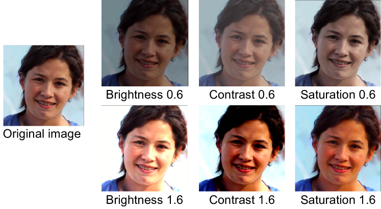
Figure 7: Examples of images processed with brightness, contrast, and saturation changes.

In this section, we evaluate the robustness in the presence of image processing operators applied to synthetic images. In particular, we consider color modifications (saturation, brightness, contrast), Gaussian blur and JPEG compression. We point out that only JPEG compression has been considered during the training of our method (see Section IV-B), while the others correspond to never-seen processing operations. For the color modifications, an example of a processed image is reported in Fig. 7 for the extreme values of the range of parameters we considered.

Fig. 6 reports the closed-set and open-set performance. BOSC has robustness similar to state-of-the-art methods for in-set samples, while it gets superior performance in the open-set case, with a gain in AU-ROC and AU-OSCR larger than 10% in all the cases. This confirms the intuition that, since the trigger images are not affected by the processing (being superimposed at test time), their features are affected to a lesser extent by processing. The most critical case is JPEG compression, notwithstanding its inclusion in the training set.

V-C Architecture vs model attribution

We also evaluated the capability of BOSC of correctly attributing to the source architecture images generated by unknown models, that is, models different than those considered during training yet sharing the same in-set architectures. In particular, the generative models used for these tests are obtained from the in-set architectures considering: i) different training strategies (for StyleGAN2, LSGM and DDPM) ii) different training datasets of real images (for Latent diffusion and Taming transformer), and iii) different image resolutions (for StyleGAN3). The details of the mismatch between the models used for training and testing are provided in Table III. With regard to the models obtained considering a mismatch in the training strategy, StyleGAN-ada refers to training with adaptive augmentation for the discriminator [51], while DDPM-ema is obtained by training with the exponential moving average strategy [52]. Finally, for LSGM, the number of stages for the training is changed, from the default value 2 to 3. In the third stage, re-training is performed by training only the SGM prior, leaving the Nouveau VAE (NVAE) component fixed. The models obtained with the 2-stage and 3-stage training are referred to as quantitative and qualitative models, respectively.

TABLE III: Closed-set and Open-set results in the case of models trained with different datasets, parameters, and training procedures (in the last line, the number in the models’ names indicates the image resolution). The underlined performance refers to the average results across different configurations.

Architecture	Type of Mismatch	Train	Test	ACC	AU-OSCR
DDPM (Config-S1)	Training Methodology	DDPM	DDPM-ema	100	85.89
StyleGAN2 (Config-S1&S2&S3)	Training Methodology	StyleGAN2-f	StyleGAN-ada	99.84	92.15
Taming Transformer (Config-S1)	Real Dataset	CelebA	FFHQ	98.20	82.53
Latent Diffusion (Config-S1&S2)	Real Dataset	CelebA	FFHQ	77.63	71.3
LSGM (Config-S2)	Training Methodology	Quantitative (2-stages)	Qualitative (3-stages)	99.60	76.46
StyleGAN3 (Config-S3)	Image Resolution	StyleGAN3 t-1024& t-ffhqu1024&r	StyleGAN3 t-ffhqu256	99.35	78.17

The last two columns of Table III report the closed-set accuracy and the AU-OSCR obtained when the system is tested with the out-of-set models. The results show that the closed-set performance is very good (Acc above 98%) in all cases, with the exception of Latent Diffusion, where we get Acc = 77.63%. The model mismatch affects the open-set performance more, and in fact, the AU-OSCR computed on the mismatched samples decreases. Performance is great in the case of Syle-GAN2 and remains pretty good also for DDPM and Taming Transformer, while they drop in the case of Latent Diffusion, LSGM and SyleGAN3. A strategy that we expect can help mitigating this issue is to include multiple models for every architecture inside the training set. Arguably, doing so should induce the system to better learn the model variability for a given generative architecture.

V-D Ablation study

We carried out an ablation study to assess the impact of each component of BOSC.

V-D1 Choice of rejection score

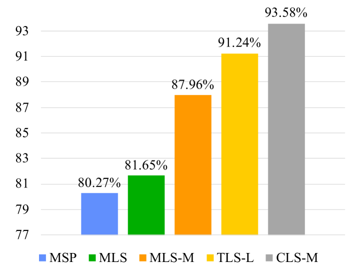
Figure 8: Average performance (AU-ROC) of out-of-set rejection of BOSC using different scores. The average is taken over the three in-set and out-of-set configurations.

The benefit of considering the trigger-based score in Eq. (5) for sample rejection with the backdoor-based network is shown in Fig. 8. In particular, the combined logit score (CLS-M) is compared with other trigger-based scores, that is, TLS-M and MLS-S (see section III-B for the definition), and also scores commonly used for OSR, which are directly obtained from the prediction output vector of $x$. In particular, we considered the maximum value of the softmax probability vector (MSP), and the maximum logit score (MLS).

TABLE IV: Ablation study on the effect of mixup augmentation.

	Accuracy	AU-ROC	AU-OSCR
Baseline	100	73.90	73.88
BOSC (w/o Mixup)	99.98	86.00	85.99
BOSC (w/- Mixup)	99.97	93.58	93.57

We see that the AU-ROC obtained with trigger-based scores (MLS-M, TLS-M, CLS-M) is much higher than the AU-ROC obtained with common scores computed on the output of clean samples (MSP and MLS). Among the three trigger-based scores, we see that TLS-M improves the performance of MLS-M from 87.96% to 91.24% on average. The performance is further improved with CLS-M (AU-ROC = 93.58%), which fully exploits the different behaviour in the presence of matched and mismatched triggers.

TABLE V: Summary of the 19 editing classes (18 + ’None’) and the configurations of in-set (11 classes) and out-of-set (8 classes).

Editing tools	Edit types
PTI	T0: None (Reconstructed)
InterfaceGAN	T1-T4: Smile, Not smile, Old, Young
StyleCLIP	Expression (T5, T6): Angry, Surprised Hair style (T7-T12): Afro, Purple_hair, Curly_hair, Mohawk, Bobcut, Bowlcut Identity change (T13-T18): Taylor_swift, Beyonce, Hilary_clinton, Trump, Zuckerberg, Depp
Configurations	In-set & Out-of-set
Config F1	In-set: T4, T1, T2, T5, T6, T7, T8, T9, T10, T11, T12 Out-of-set: T0, T3, T13, T14, T15, T16, T17, T18
Config F2	T5, T1, T2, T3, T4, T11, T12, T13, T14, T15, T18 Out-of-set: T0, T6, T7, T8, T9, T10, T16, T17
Config F3	T2, T1, T3, T4, T6, T10, T12, T15, T16, T17, T18 Out-of-set: T0, T5, T7, T8, T9, T11, T13, T14

V-D2 Mixup augmentation

We also ran some experiments to assess the benefit of the mixup augmentation strategy. Table IV reports the closed-set and open-set performance achieved by BOSC when training is carried out with and without mixup augmentation. The performance of the baseline is also reported. We see that, while the accuracy values of all the models are the same, the open-set performance improve significantly with the adoption of mixup augmentation. In particular, the gain brought by the mixup strategy in the performance of BOSC is 7.58% in both AU-ROC and AU-OSCR.

VI Application to facial editing classification

In this section, we describe the experiments we ran on an additional image forensic task, namely the open-set classification of facial attribute editing [7].

The classification of facial attribute editing consists in detecting the particular facial attribute modified by means of a conditional generative network. Possibly manipulate facial attributes, including age, gender, or expression. Classifying the manipulated attributes in facial images enables effective analysis and detection of tampered or manipulated content, ensuring the integrity and authenticity of visual data in digital environments.

VI-A GAN Face Editing Dataset and Setting

The dataset for these experiments is built as in [30]. The face images are taken from the CelebA-HQ dataset. The images are manipulated with 18 editing types: 4 facial attributes are edited with InterfaceGAN [53], and 14 facial attributes with StyleCLIP [54]. The reconstructed version of the image with no editing (’None’) by PTI [55] is also considered, for a total of 19 classes. An overview of the dataset is provided in Table V. The editing attributes are grouped into four categories: expression, ageing, hairstyle and identity change. The editing types are split into 11 in-set and 8 out-of-set classes. Three different splittings of in-set and out-of-set editing types are considered, named ’Config-F1’, ’Config-F2’ and ’Config-F3’. Fig. 9 shows an example of a manipulated face image for each edited attribute. A total number of 5992 images were taken from CelebA-HQ dataset. For each configuration, 4400 CelebA-HQ images have been used to generate the edited images used for training, 1592 for those used for testing, for a total of 83600 (4400 × 11) images for training and 30248 (1592 × 19) for testing.

The BOSC classifier was trained as described in the previous section, using the same parameters’ setting reported in Section IV-B. The 11 trigger images used for training are illustrated in Fig. 5. Regarding augmentation, we considered only horizontal flipping.

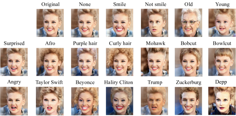
Figure 9: Examples of edited images by InterfaceGAN [53] (first row) and StyleCLIP [54] (second and third rows).

VI-B Results

TABLE VI: Performance of facial editing classification in closed-set (Accuracy) and open-set (AU-ROC, AU-OSCR). The best results are shown in bold (the second-best is underlined).

Methods	Config F1			Config F2			Config F3			Average
	Closed-set	Open-set		Closed-set	Open-set		Closed-set	Open-set		Closed-set	Open-set
	Accuracy	AU-ROC	AU-OSCR	Accuracy	AU-ROC	AU-OSCR	Accuracy	AU-ROC	AU-OSCR	Accuracy	AU-ROC	AU-OSCR
ARPL [13]	91.92	86.84	82.54	94.41	87.34	84.57	90.99	85.84	80.64	92.44	86.67	82.58
AKPF [15]	94.41	91.09	87.84	95.33	88.72	86.49	91.45	87.35	82.58	93.73	89.05	85.64
PCSSR [14]	95.33	85.60	82.77	96.40	82.60	80.63	91.87	86.23	81.39	94.53	84.81	81.60
RCSSR [14]	95.05	82.46	79.48	97.02	89.98	88.37	93.27	82.68	78.41	95.11	85.04	82.09
Res50Vit [30]	93.65	91.42	87.65	95.59	91.66	89.50	91.83	86.64	82.13	93.69	89.91	86.43
Baseline	97.21	87.85	86.66	97.91	88.22	87.24	95.09	86.10	83.92	96.74	87.39	85.94
BOSC (Ours)	96.65	92.13	90.35	97.28	91.62	90.49	94.50	88.43	85.40	96.16	90.73	88.75

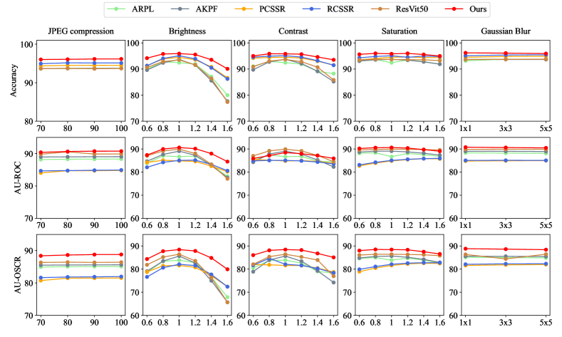
Figure 10: Robustness to image-level attacks. From left to right: JPEG compression, brightness, contrast, saturation and Gaussian blur. From top to bottom: Accuracy (closed-set) AU-ROC and AU-OSCR (open-set).

The proposed method is compared with ARPL [13], AKPF [15], PCSSR [14], RCSSR [14] (general OSR methods), and the ResVit50 method [30], which, as pointed out before, corresponds to a method specifically proposed for this task. The performance of an EfficientNet-B4 trained on the in-set classes using MLS for out-of-set detection (baseline) is also reported.

The results achieved for in-set and out-of-set samples are shown in Table VI. We see that all methods obtain AU-ROC and AU-OSCR larger than 80%, while the closed-set accuracy of the various methods ranges between 92% and 97%, with BOSC performing the best in almost all the cases. Besides, the results of all methods are stable across the various configurations. The best open-set results for the state-of-the-art are achieved by AKPF and Res50Vit, with the latter yielding the best performance. Compared to Res50Vit, BOSC achieves a small gain of 0.82% in AU-ROC and 2.32% in AU-OSCR (and a 2.47% gain in the Accuracy). We stress that Res50Vit is specialized for this task and resorts to the aid of a localization branch to focus on the face regions that are most relevant for the various editing. Therefore, the similar (slightly better) performance obtained by BOSC represents a noticeable result, also proving its generality across different image forensic tasks.

Finally, the robustness performance of the various methods against brightness, contrast, saturation, Gaussian blur and JPEG compression are reported in Fig. 10. We see that BOSC always achieves the best robustness. In the case of contrast adjustment, AKPF and Res50Vit slightly outperform BOSC in terms of out-of-set detection capability (AU-ROC). However, the overall classification performance in open set (AU-OSCR) is noticeably superior for BOSC.

VII Conclusion

We have presented a backdoor-based open-set classification (BOSC) framework for open-set synthetic image attribution. BOSC works by injecting class-specific triggers inside a portion of the images of the training set to induce the network to establish a link between class features and trigger features. Such a matching is exploited during testing for out-of-set detection by means of an ad-hoc score. The results show that the proposed method achieves better open-set performance compared to the state-of-the-art. The effectiveness of BOSC was also validated on the open-set classification of synthetic facial editing, confirming the superiority over the state-of-the-art also on this task, as well as the generality of the approach.

Future work will focus on investigating the impact of the choice of trigger images on the results and on optimizing the triggers for a given classification task. We also plan to apply BOSC to other open-set classification tasks, also beyond image forensics, to validate its effectiveness for general OSR image classification tasks.

References

- [1] A. Vahdat, and J. Kautz, “NVAE: A deep hierarchical variational autoencoder,” in Advances in Neural Information Processing Systems, vol. 33, 2020, pp. 19667–19679.
- [2] T. Karras, S. Laine, M. Aittala, J. Hellsten, J. Lehtinen, and T. Aila, “Analyzing and improving the image quality of stylegan,” in Proc. IEEE Conf. Comput. Vis. Pattern Recognit. (CVPR), Jun. 2020, pp. 8110–8119.
- [3] T. Karras, M. Aittala, S. Laine, E. Härkönen, J. Hellsten, J. Lehtinen, and T. Aila, “Alias-free generative adversarial networks,” in Advances in Neural Information Processing Systems, vol. 34, 2021, pp. 852–863.
- [4] J. Ho, A. Jain, and P. Abbeel, “Denoising diffusion probabilistic models,” in Advances in Neural Information Processing Systems, vol. 33, 2020, pp. 6840–6851.
- [5] X. Zhang, S. Karaman, and S. F. Chang, “ Detecting and simulating artifacts in gan fake images,” in Proc. IEEE international workshop on information forensics and security (WIFS), 2019, pp. 1–6.
- [6] M. Goebel, L. Nataraj,, T. Nanjundaswamy,T.M. Mohammed, S. Chandrasekaran, and B.S. Manjunath, “Non-linear estimation is easy,” Electronic Imaging, vol. 33, pp. 1–11, 2021.
- [7] J. Wang, B. Tondi, and M. Barni, “Classification of synthetic facial attributes by means of hybrid classification/localization patch-based analysis,” in ICASSP 2023-2023 IEEE International Conference on Acoustics, Speech and Signal Processing (ICASSP), Jun. 2023, pp. 1–5.
- [8] F. Marra, D. Gragnaniello, L. Verdoliva, and G. Poggi, “Do GANs leave artificial fingerprints?,” in Proc. IEEE Conf. on Multimedia Information Processing and Retrieval (MIPR), 2019, pp. 506–511.
- [9] N. Yu, L. Davis, and M. Fritz, “Attributing Fake Images to GANs: Learning and Analyzing GAN Fingerprints,” in Proc. IEEE/CVF Int. Conf. Comput. Vis. (ICCV), Oct. 2019, pp. 7556–7566.
- [10] N. Yu, V. Skripniuk, S. Abdelnabi, and M. Fritz, “Artificial Fingerprinting for Generative Models: Rooting Deepfake Attribution in Training Data,” in Proc. IEEE/CVF Int. Conf. Comput. Vis. (ICCV), Oct. 2021, pp. 14448–14457.
- [11] T. Yang, Z. Huang, J. Cao, L. Li, and X. Li, “Deepfake network architecture attribution,” in Proceedings of the AAAI Conference on Artificial Intelligence, vol. 36, no. 4, pp. 4662–4670, 2022.
- [12] T. Bui, N. Yu, and J. Collomosse, “Repmix: Representation mixing for robust attribution of synthesized images,” in Proc. of the European Conf. on Comput. Vis. (ECCV), Sept. 2022, pp. 146–163.
- [13] G. Chen, P. Peng, X. Wang, and Y. Tian, “Adversarial reciprocal points learning for open set recognition,” IEEE Trans. Pattern Anal. Mach. Intell., vol. 44, no. 11, pp. 8065–8081, 2021.
- [14] H. Huang, Y. Wang, Q. Hu, and M. M. Cheng, “Class-specific semantic reconstruction for open set recognition,” IEEE Trans. Pattern Anal. Mach. Intell., vol. 45, no. 4, pp. 4214–4228, 2022.
- [15] Z. Xia, P. Wang, G. Dong, and H. Liu, “Adversarial kinetic prototype framework for open set recognition,” IEEE Trans. Neural Networks and Learning Systems, 2023.
- [16] S. Vaze, K. Han, A. Vedaldi, and A. Zisserman, “Open-set recognition: A good closed-set classifier is all you need?,” in Int. Conf. on Learning Representations (ICLR), 2022.
- [17] Z. Y. Ge, S. Demyanov, Z. Chen, and R. Garnavi, “Generative openmax for multi-class open set classification,” 2017, arXiv:1707.07418.
- [18] W. Moon, J. Park, H. S. Seong, C. H. Cho, and J. P. Heo, “Difficulty-aware simulator for open set recognition,” in Proc. of the European Conf. on Comput. Vis. (ECCV), Sept. 2020, pp. 365–381.
- [19] W. Guo, B. Tondi, and M. Barni, “An overview of backdoor attacks against deep neural networks and possible defences,” IEEE Open Journal of Signal Processing, 2022.
- [20] T. Gu, B. Dolan-Gavitt, and S. Garg, “Badnets: Identifying vulnerabilities in the machine learning model supply chain,” 2017, arXiv:1708.06733.
- [21] W. Scheirer, A. Rocha, A. Sapkota, and T. Boult, “Toward Open Set Recognition,” IEEE Trans. Pattern Anal. Mach. Intell., vol. 35, no. 7, pp. 1757–1772, 2013.
- [22] G. Gavarini, D. Stucchi, A. Ruospo, G. Boracchi, and E. Sanchez, “ Open-set recognition: an inexpensive strategy to increase dnn reliability,” in 2022 IEEE 28th International Symposium on On-Line Testing and Robust System Design (IOLTS), 2022, pp. 1–7.
- [23] C. Chow, “On optimum recognition error and reject tradeoff,” IEEE Transactions on information theory, vol. 16, no. 1, pp. 41–46, 1970.
- [24] W. Liu, X. Wang, J. Owens, and Y. Li, “Energy-based out-of-distribution detection,” in Proc. of the Advances in Neural Information Processing Systems, vol. 33, pp. 21464–21475, 2020.
- [25] H. M. Yang, X. Y. Zhang, F. Yin, and C. L. Liu, “Robust classification with convolutional prototype learning,” in Proc. IEEE Conf. Comput. Vis. Pattern Recognit. (CVPR), Jun. 2018, pp. 3474–3482.
- [26] G. Chen, L. Qiao, Y. Shi, P. Peng, J. Li, T. Huang, S. Pu, and Y. Tian, “Learning open set network with discriminative reciprocal points,” in Proc. of the European Conf. on Comput. Vis. (ECCV), Sept. 2020, pp. 507–522.
- [27] R. Yoshihashi, W. Shao, R. Kawakami, S. You, M. Iida, and T. Naemura, “Classification-Reconstruction Learning for Open-Set Recognition,” in Proc. IEEE Conf. Comput. Vis. Pattern Recognit. (CVPR), Jun. 2019, pp. 4016–4025.
- [28] P. Oza, and V. M. Patel, “C2ae: Class conditioned auto-encoder for open-set recognition,” in Proc. IEEE Conf. Comput. Vis. Pattern Recognit. (CVPR), Jun. 2019, pp. 2307–2316.
- [29] X. Sun, Z. Yang, C. Zhang, K. V. Ling, and G. Peng, “Conditional gaussian distribution learning for open set recognition,” in Proc. IEEE Conf. Comput. Vis. Pattern Recognit. (CVPR), Jun. 2020, pp. 13480–13489.
- [30] J. Wang, O. Alamayreh, B. Tondi, and M. Barni, “Open Set Classification of GAN-based Image Manipulations via a ViT-based Hybrid Architecture,” in Proc. IEEE Conf. Comput. Vis. Pattern Recognit. (CVPR), Jun. 2023, pp. 953–962.
- [31] C. Kim, Y. Ren, and Y. Yang, “Decentralized attribution of generative models,” in InInternational Conference on Learning Representations, Oct., 2020.
- [32] N. Yu, V. Skripniuk, D. Chen, L. Davis, M. Fritz, “Responsible disclosure of generative models using scalable fingerprinting,” 2020, arXiv:2012.08726.
- [33] T. Yang, J. Cao, Q. Sheng, J. Ji, X. Li, and S. Tang, “Learning to disentangle gan fingerprint for fake image attribution,” 2021, arXiv:2106.08749v1.
- [34] J. Frank, T. Eisenhofer, L. Schönherr, A. Fischer, D. Kolossa, and T. Holz, “Leveraging frequency analysis for deep fake image recognition,” in International conference on machine learning, pp. 3247–3258, 2020.
- [35] S. Girish, S. Suri, S. S. Rambhatla, and A. Shrivastava, “Towards discovery and attribution of open-world gan generated images,” in Proc. IEEE Conf. Comput. Vis. Pattern Recognit. (CVPR), Jun. 2021, pp. 14094–14103.
- [36] Z. Sun, S. Chen, T. Yao, B. Yin, R. Yi, S. Ding, and L. Ma, “Contrastive Pseudo Learning for Open-World DeepFake Attribution,” in Proc. IEEE Conf. Comput. Vis. Pattern Recognit. (CVPR), Jun. 2023, pp. 20882–20892.
- [37] H. M. Yang, X. Y. Zhang, F. Yin, and C. L. Liu, “Progressive Open Space Expansion for Open-Set Model Attribution,” in Proc. IEEE Conf. Comput. Vis. Pattern Recognit. (CVPR), Jun. 2023, pp. 15856–15865.
- [38] S. Fang, T. D. Nguyen, and M. C. Stamm, “Open Set Synthetic Image Source Attribution,” 2023, arXiv:2308.11557.
- [39] T. Yang, J. Cao, D. Wang, and C. Xu, “Fingerprints of Generative Models in the Frequency Domain,” 2023, arXiv:2307.15977.
- [40] L. Abady, J. Wang, B. Tondi, and M. Barni, “A Siamese-based verification system for open-set architecture attribution of synthetic images,” Pattern Recognition Letter, vol. 180, 2024.
- [41] H. Zhang, M. Cisse, Y. N. Dauphin, and D. Lopez-Paz, “mixup: Beyond empirical risk minimization,” in InInternational Conference on Learning Representations, Feb. 2018.
- [42] A. Brock, J. Donahue, and K. Simonyan, “Large scale GAN training for high fidelity natural image synthesis,” in International Conference on Learning Representations, 2018.
- [43] D. Berthelot, T. Schumm, and L. Metz , “Began: Boundary equilibrium generative adversarial networks,” 2017, arXiv:1703.10717.
- [44] T. Karras, T. Aila, S. Laine, and J. Lehtinen, “Progressive growing of gans for improved quality, stability, and variation,” in International Conference on Learning Representations, 2018.
- [45] Y. Choi, Y. Uh, J. Yoo, and J. W. Ha , “Stargan v2: Diverse image synthesis for multiple domains,” in Proc. IEEE Conf. Comput. Vis. Pattern Recognit. (CVPR), Jun. 2020, pp. 8188–8197.
- [46] R. Rombach, A. Blattmann, D. Lorenz, P. Esser, and B. Ommer, “High-resolution image synthesis with latent diffusion models,” in Proc. IEEE Conf. Comput. Vis. Pattern Recognit. (CVPR), Jun. 2022, pp. 10684–10695.
- [47] A. Vahdat, K. Kreis, and J. Kautz, “Score-based generative modeling in latent space,” in Advances in Neural Information Processing Systems, vol. 34, 2021, pp. 11287–11302.
- [48] P. Esser, R. Rombach, and B. Ommer, “Taming transformers for high-resolution image synthesis,” in Proc. IEEE Conf. Comput. Vis. Pattern Recognit. (CVPR), Jun. 2021, pp. 12873–12883.
- [49] T. Karras, S. Laine, and T. Aila, “A style-based generator architecture for generative adversarial networks,” in Proc. IEEE Conf. Comput. Vis. Pattern Recognit. (CVPR), Jun. 2019, pp. 4401–4410.
- [50] Z. Liu, P. Luo, X. Wang, and X. Tang, “Deep Learning Face Attributes in the Wild,” in Proc. IEEE/CVF Int. Conf. Comput. Vis. (ICCV), 2015, pp. 3730–3738.
- [51] T. Karras, M. Aittala, J. Hellsten, S. Laine, J. Lehtinen, and T. Aila, “Training Generative Adversarial Networks with Limited Data,” in Advances in neural information processing systems, vol. 33, 2020, pp. 12104–12114.
- [52] D. Busbridge, J. Ramapuram, P. Ablin, T., Likhomanenko, E. G., Dhekane, X., Suau Cuadros, and R. Webb, “How to scale your ema,” in Advances in Neural Information Processing Systems, vol. 36, 2024.
- [53] Y. Shen, J. Gu, X. Tang, and B. Zhou , “Interpreting the latent space of gans for semantic face editing,” in Proc. IEEE Conf. Comput. Vis. Pattern Recognit. (CVPR), Jun. 2020, pp. 9243–9252.
- [54] O Patashnik, Z Wu, E Shechtman, D Cohen-Or, D Lischinskia, “Styleclip: Text-driven manipulation of stylegan imagery,” in Proc. IEEE/CVF Int. Conf. Comput. Vis. (ICCV), Oct. 2021, pp. 2085–2094.
- [55] D. Roich, R. Mokady, A. H. Bermano, and D. Cohen-Or, “Pivotal tuning for latent-based editing of real images,” ACM Transactions on graphics (TOG), 2022.