FIFO-Diffusion: Generating Infinite Videos from Text without Training

Abstract

We propose a novel inference technique based on a pretrained diffusion model for text-conditional video generation. Our approach, called FIFO-Diffusion, is conceptually capable of generating infinitely long videos without additional training. This is achieved by iteratively performing diagonal denoising, which concurrently processes a series of consecutive frames with increasing noise levels in a queue; our method dequeues a fully denoised frame at the head while enqueuing a new random noise frame at the tail. However, diagonal denoising is a double-edged sword as the frames near the tail can take advantage of cleaner ones by forward reference but such a strategy induces the discrepancy between training and inference. Hence, we introduce latent partitioning to reduce the training-inference gap and lookahead denoising to leverage the benefit of forward referencing. Practically, FIFO-Diffusion consumes a constant amount of memory regardless of the target video length given a baseline model, while well-suited for parallel inference on multiple GPUs. We have demonstrated the promising results and effectiveness of the proposed methods on existing text-to-video generation baselines. Generated video samples and source codes are available at our project page.

(a) "A spectacular fireworks display over Sydney Harbour, 4K, high resolution."
(b) "An astronaut walking on the moon’s surface, high-quality, 4K resolution."
(c) "A colony of penguins waddling on an Antarctic ice sheet, 4K, ultra HD."

Figure 1: Illustration of 10K-frame long videos generated by FIFO-Diffusion based on a pretrained text-conditional video generation model, VideoCrafter2 (Chen et al., 2024). The number at the top-left corner of each image indicates the frame index. The results clearly show that FIFO-Diffusion can generate extremely long videos effectively based on the model trained on short clips (16 frames) without quality degradation while preserving the dynamics and semantics of scenes.

1 Introduction

Diffusion probabilistic models have achieved significant success in generating images (Ho et al., 2020; Song et al., 2021b; Dhariwal & Nichol, 2021; Rombach et al., 2022). On top of the success in the image domain, there has been rapid progress in the generation of videos (Ho et al., 2022; Singer et al., 2022; Zhou et al., 2022; Wang et al., 2023b).

Despite the progress, long video generation still lags behind compared to image generation. One reason is that video diffusion models (VDMs) often consider a video as a single 4D tensor with an additional axis corresponding to time, which prevents the models from generating videos at scale. An intuitive approach to generating a long video is autoregressive generation, which iteratively predicts a future frame given the previous ones. However, in contrast to the transformer-based models (Hong et al., 2023; Villegas et al., 2023), diffusion-based models cannot directly adopt the autoregressive generation strategy due to the heavy computational costs incurred by iterative denoising steps for a single frame generation. Instead, many recent works (Ho et al., 2022; He et al., 2022; Voleti et al., 2022; Luo et al., 2023; Chen et al., 2023b; Blattmann et al., 2023) adopt a chunked autoregressive generation strategy, which predicts several frames in parallel conditioned on few preceding ones, consequently reducing computational burden. While these approaches are computationally tractable, they often leads to temporal inconsistency and discontinuous motion, especially between the chunks predicted separately, since the model captures a limited temporal context available in the last few—only one or two in practice—frames.

The proposed inference technique, FIFO-Diffusion, realizes the long video generation even without training. It facilitates generating videos with arbitrary lengths, based on a diffusion model for video generation pretrained on short clips. Moreover, it effectively alleviates the limitations of the chunked autoregressive method by enabling every frame to refer to a sufficient number of preceding frames.

Our approach generates frames through diagonal denoising (Section 4.1) in a first-in-first-out manner using a queue, which maintains a sequence of frames with different—monotonically increasing—noise levels over time. At each step, a completely denoised frame at the head is popped out from the queue while a new random noise image is pushed back at the tail. Diagonal denoising offers both advantage and disadvantage; noisier frames benefit from referring to cleaner ones at preceding diffusion steps while the model may suffer from training-inference gap in terms of the noise levels of concurrently processed frames. To overcome this limitation and embrace the advantage of diagonal denoising, we propose latent partitioning (Section 4.2) and lookahead denoising (Section 4.3). Latent partitioning constrains the range of noise levels in the noisy input images and enhances video quality by finer discretization of diffusion process. Additionally, lookahead denoising enhances the capacity of the baseline model, providing even more accurate noise prediction. Furthermore, both latent partitioning and lookahead denoising offer parallelizability on multiple GPUs.

Our main contributions are summarized below.

• We propose FIFO-Diffusion through diagonal denoising, which is a training-free video generation technique for VDMs trained on short clips. Our approach allows each frame to refer to a sufficient number of preceding frames and facilitates the generation of arbitrarily long videos.

• We introduce latent partitioning and lookahead denoising, which enhances generation quality and demonstrate the effectiveness of those two techniques theoretically and empirically.

• FIFO-Diffusion utilizes a constant amount of memory regardless of the generating video length given a baseline model, while it is straightforward to perform parallel inference on multiple GPUs.

• Our experiments on four strong baselines, based on the U-Net (Ronneberger et al., 2015) or DiT (Peebles & Xie, 2023) architectures, show that FIFO-Diffusion generates extremely long videos including natural motion without degradation on quality over time.

2 Related work

This section discusses existing diffusion-based generative models for videos and summarize long video generation techniques.

2.1 Video diffusion models

Video generation often relies on diffusion models  (Ho et al., 2022; Singer et al., 2022; Zhou et al., 2022; Wang et al., 2023b; Chen et al., 2023a). Among the diffusion-based techniques, VDM (Ho et al., 2022) modifies the structure of U-Net (Ronneberger et al., 2015) and proposes a 3D U-Net architecture to consider temporal information for denoising. On the other hand, Make-A-Video (Singer et al., 2022) adds 1D temporal convolution layers after 2D spatial counterparts to approximate 3D convolutions. Such an architecture allows it to understand visual-textual relations by first training spatial layers with image-text pairs followed by 1D temporal layers for temporal context in videos. Recently, (Peebles & Xie, 2023) introduce transformer architecture, referred to as DiT, for diffusion models. Additionally, there are several open-sourced text-to-video models (Wang et al., 2023b; Chen et al., 2023a; Wang et al., 2023c; Chen et al., 2024), which are trained on large-scale text-image and text-video datasets.

2.2 Long video generation

He et al. (2022); Voleti et al. (2022); Yin et al. (2023); Harvey et al. (2022); Blattmann et al. (2023); Chen et al. (2023b) train models to predict masked frames given visible ones for generating long videos. NUWA-XL (Yin et al., 2023) proposes a hierarchical approach, where a global diffusion model generates sparse key frames while local diffusion models interpolate between them. However, the hierarchical framework exhibits its limitations in generating infinitely long videos. On the other hand, models like LVDM (He et al., 2022) and MCVD (Voleti et al., 2022) autoregressively predict successive frames given few initial frames, while FDM (Harvey et al., 2022) and SEINE (Chen et al., 2023b) generalize the masking strategies to perform prediction or interpolation. While autoregressive frameworks can generate infinitely long video, they often suffer from quality degradation caused by error accumulation and lack of temporal consistency across frames. LGC-VD (Yang et al., 2023) considers both global and local contexts for model construction to address the limitations.

Wang et al. (2023a); Qiu et al. (2023) propose tuning-free long video generation techniques. Gen-L-Video (Wang et al., 2023a) views a video as overlapped short clips and suggests temporal co-denoising, which averages multiple predictions for one frame. FreeNoise (Qiu et al., 2023) employs window-based attention fusion to sidestep attention scope issue and proposes local noise shuffle units for the initialization of long video. However, it requires memory proportional to the video length to compute cross-attention, making it difficult to generate infinitely long videos.

3 Text-to-video diffusion models

We summarize the basic idea of text-conditional video generation techniques. They consist of a few key components: an encoder $\text{Enc}(\cdot)$, a decoder $\text{Dec}(\cdot)$, and a noise prediction network $\bm{\epsilon}_{\theta}(\cdot)$. They learn the distribution of videos corresponding to text conditions, denoted by $\bm{v}\in\mathbb{R}^{f\times H\times W\times 3}$, where $f$ is the number of frames and $H\times W$ indicates the image resolution. The encoder projects each frame onto the latent space of image while the decoder reconstructs the frame from the latent. A video latent $\mathbf{z}_{0}=\text{Enc}(\bm{v})=[\bm{z}^{1}_{0};\text{\makebox[5.0pt][c]{.\hfil.\hfil.}\thinspace};\bm{z}^{f}_{0}]\in\mathbb{R}^{f\times h\times w\times c}$ is obtained by concatenating projected frames and the latent diffusion model is trained to denoise its perturbed version, $\mathbf{z}_{t}$. For the noise $\bm{\epsilon}\sim\mathcal{N}(\mathbf{0},\mathbf{I})$, the diffusion time step $t\sim\mathcal{U}([1,\text{\makebox[5.0pt][c]{.\hfil.\hfil.}\thinspace},T])$, and text condition $\bm{c}$, the model is trained to minimize the following loss:

$$\mathbb{E}_{\bm{v},\bm{\epsilon},t}\left[||\bm{\epsilon}_{\theta}(\mathbf{z}_{t};\bm{c},t)-\bm{\epsilon}||\right],$$ (1)

where $\mathbf{z}_{t}=s_{t}\mathbf{z}_{0}+\sigma_{t}\bm{\epsilon}$, given predefined constants $\{s_{t}\}_{t=0}^{T}$ and $\{\sigma_{t}\}_{t=0}^{T}$ satisfying $s_{0}=1$, $\sigma_{0}=0$ and $\sigma_{T}/s_{T}\gg 1$.

For a time step schedule, $0=\tau_{0}<\tau_{1}<\text{\makebox[5.0pt][c]{.\hfil.\hfil.}\thinspace}<\tau_{S}=T$, initialized by a diffusion scheduler, the model generates a video by iteratively denoising $\mathbf{z}_{\tau_{S}}^{\text{vdm}}=~{}[\bm{z}_{\tau_{S}}^{1};\text{\makebox[5.0pt][c]{.\hfil.\hfil.}\thinspace};\bm{z}_{\tau_{S}}^{f}]\sim\mathcal{N}(\mathbf{0},\mathbf{I})$ for $S$ times using a sampler $\Phi(\cdot)$ such as the DDIM sampler. Each denoising step is expressed as follows:

$$[\bm{z}_{\tau_{t-1}}^{1};\text{\makebox[5.0pt][c]{.\hfil.\hfil.}\thinspace};\bm{z}_{\tau_{t-1}}^{f}]=\Phi([\bm{z}_{\tau_{t}}^{1};\text{\makebox[5.0pt][c]{.\hfil.\hfil.}\thinspace};\bm{z}_{\tau_{t}}^{f}],[\tau_{t};\text{\makebox[5.0pt][c]{.\hfil.\hfil.}\thinspace};\tau_{t}],\bm{c};\bm{\epsilon}_{\theta}),$$ (2)

where $\bm{z}_{\tau_{t}}^{i}$ denotes the $i^{\text{th}}$ frame latent at time step $\tau_{t}$.

4 FIFO-Diffusion

This section discusses how FIFO-Diffusion generates long videos consisting of $N$ frames using a pretrained model only for $f$ frames ($f\ll N$). The proposed approach iteratively employs diagonal denoising (Section 4.1) over a fixed number of frames with different levels of noise. Our method also incorporates latent partitioning (Section 4.2) and lookahead denoising (Section 4.3) to improve diagonal denoising of FIFO-Diffusion.

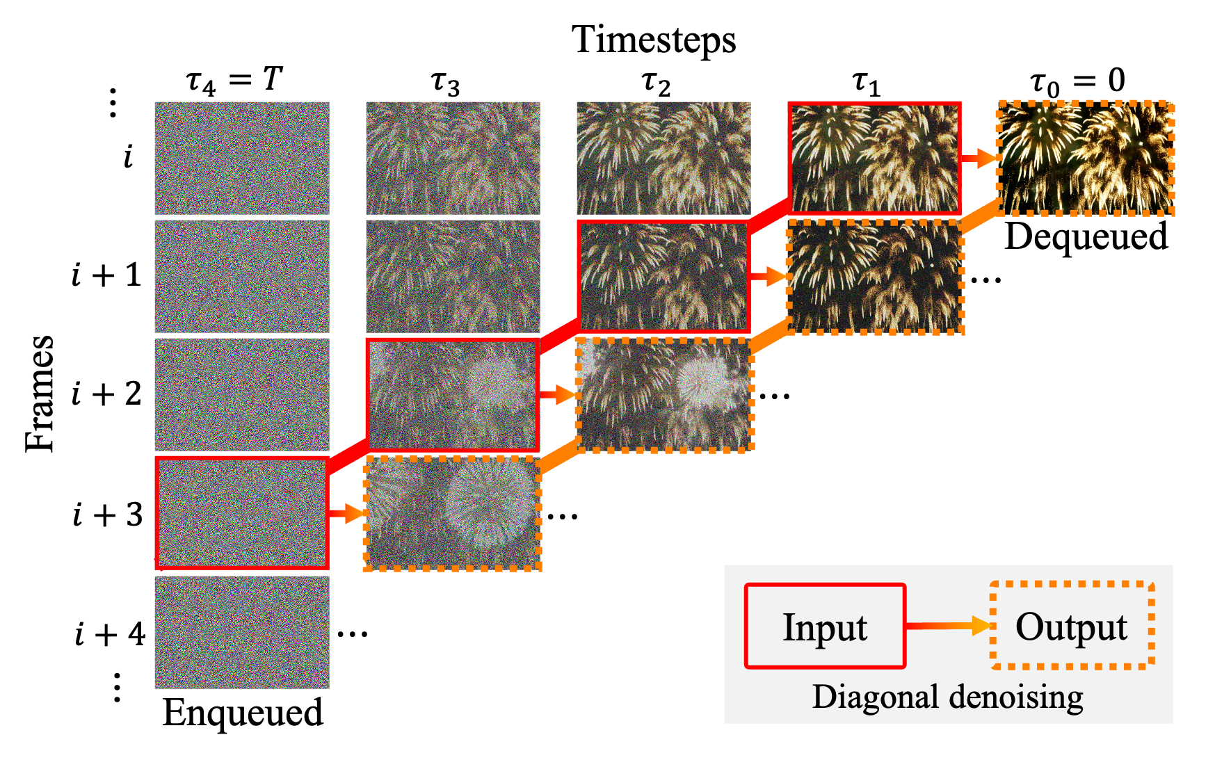
Figure 2: Illustration of diagonal denoising with $f=4$. The frames surrounded by solid lines are model inputs while frames surrounded by dotted line are their denoised version. After denoising, the fully denoised instance at the top-right corner is dequeued while random noise is enqueued.

4.1 Diagonal denoising

Diagonal denoising processes a series of consecutve frames with increasing noise levels as depicted in Figure 2. To be specific, for the time step schedule $0=\tau_{0}<\tau_{1}<\text{\makebox[5.0pt][c]{.\hfil.\hfil.}\thinspace}<\tau_{f}=T$, each denoising step is defined as following:

$$[\bm{z}_{\tau_{0}}^{1};\text{\makebox[5.0pt][c]{.\hfil.\hfil.}\thinspace};\bm{z}_{\tau_{f-1}}^{f}]=\Phi([\bm{z}_{\tau_{1}}^{1};\text{\makebox[5.0pt][c]{.\hfil.\hfil.}\thinspace};\bm{z}_{\tau_{f}}^{f}],[\tau_{1};\text{\makebox[5.0pt][c]{.\hfil.\hfil.}\thinspace};\tau_{f}],\bm{c};\bm{\epsilon}_{\theta}).$$ (3)

Note that the diagonal latents $\{\bm{z}_{\tau_{i}}^{i}\}_{i=1}^{f}$ are stored in a queue, Q, and diagonal denoising jointly considers different noise levels of $[\tau_{1};\text{\makebox[5.0pt][c]{.\hfil.\hfil.}\thinspace};\tau_{f}]$, in contrast to Equation 2.

Algorithm 1 in Appendix C illustrates how FIFO-Diffusion works. Starting from initial latents $\{\bm{z}_{\tau_{i}}^{i}\}_{i=1}^{f}$, after each denoising step, the foremost frame is dequeued as it arrives at the noise level $\tau_{0}=0$, and the new latent at noise level $\tau_{f}$ is enqueued. As a result, the model generates frames in a first-in-first-out manner. The initial latents are corrupted versions of the frames generated by the baseline model. Since the model always takes $f$ frames as an input regardless of the target video length, FIFO-Diffusion can generate an arbitrary number of frames without memory concerns. Specifically, generating $N~{}(\gg f)$ frames of video consumes $\mathcal{O}(f)$ memory (see Table 1), which remains independent of $N$, and the model completes one frame per each iteration.

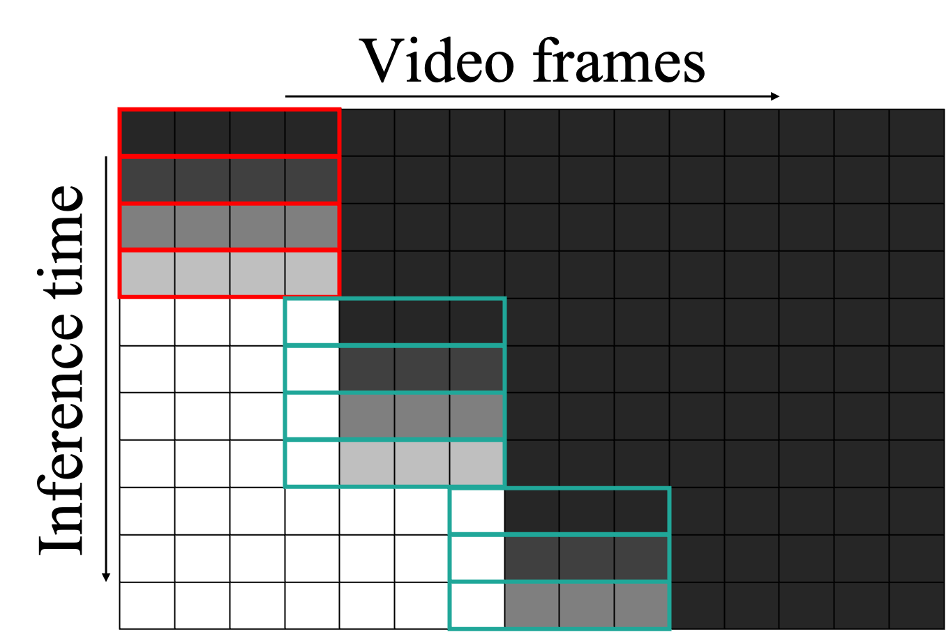
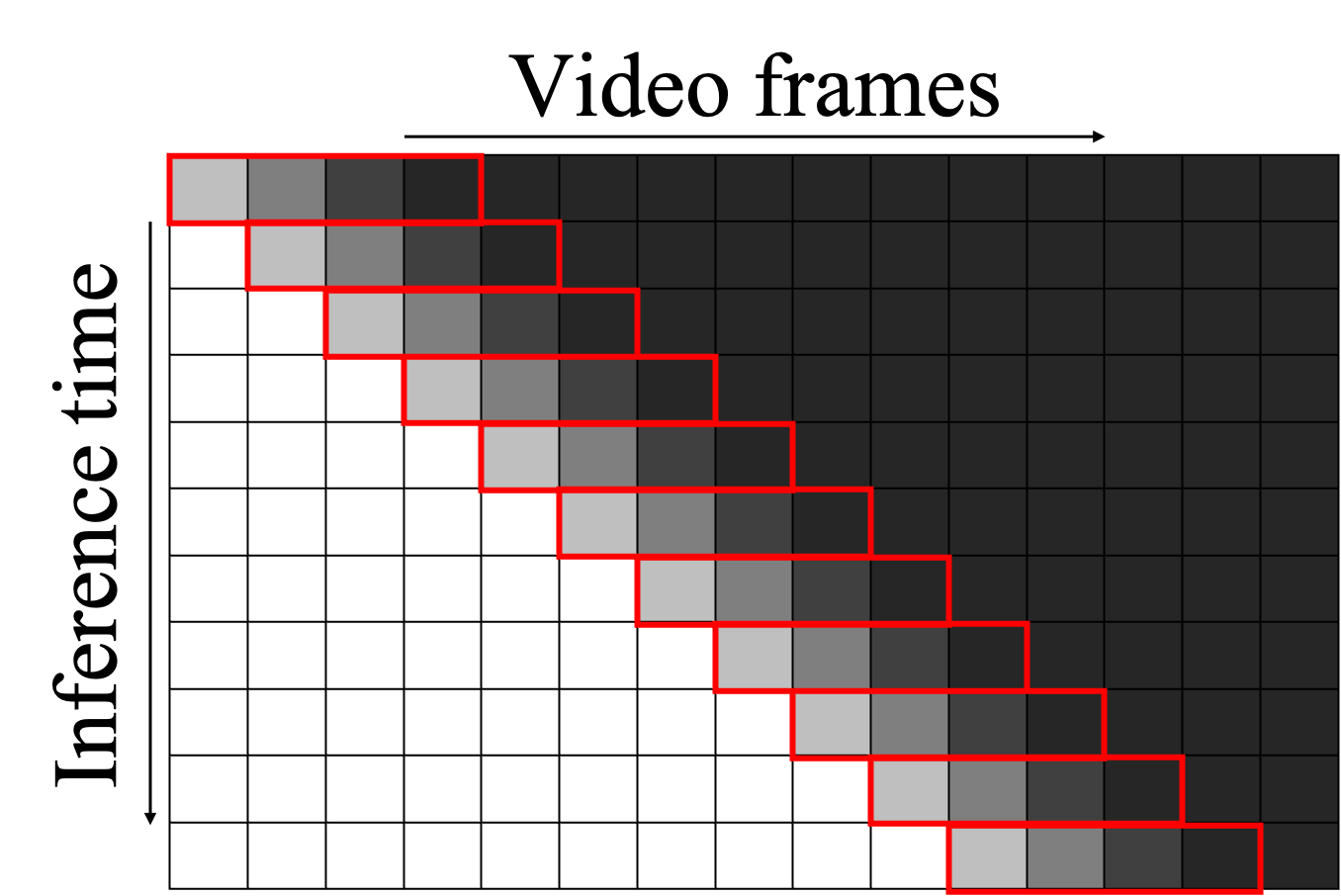
(a) Chunked autoregressive	(b) FIFO-Diffusion

Figure 3: Comparison between the chunked autoregressive methods and FIFO-Diffusion proposed for long video generation. The random noises (black) are iteratively denoised to image latents (white) by the models. The red boxes indicate the denoising network in the pretrained base model while the green boxes denote the prediction network obtained by additional training.

FIFO-Diffusion excels in generating consistent videos by sequentially propagating context to later frames. Figure 3 illustrates the conceptual difference between chunked autoregressive methods (Ho et al., 2022; He et al., 2022; Voleti et al., 2022; Luo et al., 2023; Chen et al., 2023b; Blattmann et al., 2023) and our approach. The former often fails to maintain long-term context across the chunks since their conditioning—only the last generated frame—lacks contextual information propagated from previous frames. However, in FIFO-Diffusion, the model shifts through the frame sequence with a stride 1, allowing each frame to reference a sufficient number of previous frames throughout the generation process. This facilitates the model to naturally extend the local consistency of a few frames to longer sequence. Furthermore, FIFO-Diffusion does not require subnetworks or additional training; it depends only on a base model. It differs from existing autoregressive methods, which require an additional prediction model or fine-tuning for masked frame outpainting.

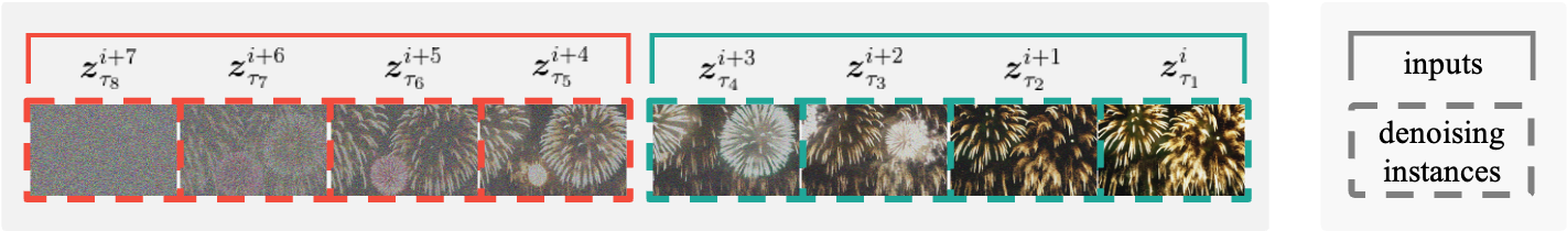
(a) Latent partitioning

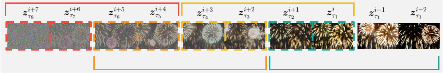
(b) Lookahead denoising

Figure 4: Illustration of latent partitioning and lookahead denoising where $f=4$ and $n=2$. (a) Latent partitioning divides the diffusion process into $n$ parts to reduce the maximum noise level difference. (b) Lookahead denoising on (a) enables all frames to be denoised with an adequate number of former frames at the expense of two times more computation than (a).

4.2 Latent partitioning

While diagonal denoising enables infinitely long video generation, it causes a training-inference gap as the model is trained to denoise all frames with the same noise levels. To address this, we aim to reduce the noise level differences in the input latents by increasing the length of the queue $n$ times (from $f$ to $nf$ with $n>1$), partitioning it into $n$ blocks, and processing each block independently. Note that increasing the queue length also increases the discretization steps of the diffusion process.

Algorithm 2 in Appendix C provides the procedure of FIFO-Diffusion with latent partitioning. Let a queue $Q$ be an ordered collection of diagonal latents $\{\bm{z}_{\tau_{i}}^{i}\}_{i=1}^{nf}$, where each latent $\bm{z}_{\tau_{i}}^{i}$ is from the diffusion time step $\tau_{i}$. Then, we partition $Q$ into $n$ blocks, $\{\text{ {Q}}_{k}\}_{k=0}^{n-1}$, of equal size $f$, and each block $Q_{k}$ contains the latents at $\bm{\tau}_{k}\equiv\{\tau_{kf+1},\dots,\tau_{(k+1)f}\}$. Afterwards, we apply diagonal denoising to each block in a divide-and-conquer manner (See Figure 4 (a)). For $k=0,\text{\makebox[5.0pt][c]{.\hfil.\hfil.}\thinspace},n-1$, each denoising step updates the queue as follows:

$$\text{ {Q}}_{k}\leftarrow\Phi(\text{ {Q}}_{k},\bm{\tau}_{k},\bm{c};\bm{\epsilon}_{\theta}).$$ (4)

To initiate the FIFO-Diffusion process with latent partitioning, we need $nf$ initial diagonal latents. However, since the baseline models can only generate $f$ frames, $\{\bm{z}_{\tau_{0}}^{\text{ref},i}\}_{i=1}^{f}$, we exploit them to construct $nf$ latents. Specifically, the last $f$ latents are corrupted versions of $\{\bm{z}_{\tau_{0}}^{\text{ref},i}\}_{i=1}^{f}$, while the first $(n-1)f$ latents are derived by corrupting the repeated $\bm{z}_{\tau_{0}}^{\text{ref},0}$, serving as dummy latents.

Latent partitioning offers three key advantages over diagonal denoising. First, it significantly reduces the maximum noise level difference between the latents from $|\sigma_{\tau_{nf}}-\sigma_{\tau_{1}}|$ to $\max_{k}{|\sigma_{\tau_{(k+1)f}}-\sigma_{\tau_{kf+1}}}|$. This effectiveness is demonstrated theoretically in Theorem 4.5 and empirically in Table 2. Second, it can save time by facilitating parallelized inference across multiple GPUs (see Table 1). This feature is exclusive to our method, as each partitioned block can be processed independently. Lastly, it allows the diffusion process to utilize a large number of inference steps, $nf$ ($n\geq 2$), reducing discretization error during inference. We now provide Theorem 4.5 showing that the gap incurred by diagonal denoising is linearly bounded by the maximum noise level difference, implying we can reduce the error by narrowing the noise level differences of model inputs.

Definition 4.1.

We define $\mathbf{z}^{\text{vdm}}_{t}=[\bm{z}_{t}^{1};\text{\makebox[5.0pt][c]{.\hfil.\hfil.}\thinspace};\bm{z}_{t}^{f}]$, where $\bm{z}_{t}^{i}$ is the latent of the $i^{\text{th}}$ frame at time step $t$. Further, $\mathbf{z}^{\text{diag}}=[\bm{z}_{\tau_{1}}^{1};\text{\makebox[5.0pt][c]{.\hfil.\hfil.}\thinspace};\bm{z}_{\tau_{f}}^{f}]$ and $\bm{\tau}^{\text{diag}}=[\tau_{1};\text{\makebox[5.0pt][c]{.\hfil.\hfil.}\thinspace};\tau_{f}]$ are diagonal latents and corresponding time steps with $s=\tau_{1}<\text{\makebox[5.0pt][c]{.\hfil.\hfil.}\thinspace}<\tau_{f}=t$.

Definition 4.2.

Following Karras et al. (2022), we consider $s_{t}=1$ and $\sigma_{t}=ct$ for some constant $c$ and corresponding ODE:

$$d\mathbf{z}_{t}^{\text{vdm}}=c\cdot\bm{\epsilon}(\mathbf{z}^{\text{vdm}}_{t},t\cdot\bm{1})dt,$$ (5)

for $\bm{1}=[1;\text{\makebox[5.0pt][c]{.\hfil.\hfil.}\thinspace};1]$. Note that $\bm{\epsilon}(\cdot)$ is the scaled score function $-\sigma\nabla_{\mathbf{z}}\log p(\cdot)$.

Definition 4.3.

$\bm{\epsilon}_{\theta}(\cdot)^{i}$ is the $i^{\text{th}}$ element of $\bm{\epsilon}_{\theta}(\cdot)$ and $\bm{\epsilon}(\cdot)^{i}$ is the $i^{\text{th}}$ element of $\bm{\epsilon}(\cdot)$.

Lemma 4.4.

If $\bm{\epsilon}(\cdot)$ is bounded, then

$$||\bm{z}_{t}^{i}-\bm{z}_{s}^{i}||=O(|t-s|)~{}~{}\text{for}~{}~{}\forall i.$$

Proof.

Refer to Section A.1. ∎

Theorem 4.5.

Assume the system satisfies the following two hypotheses:

(H1) $$\bm{\epsilon}(\cdot)$$ is bounded.

(H2) The diffusion model $$\bm{\epsilon}_{\theta}(\cdot) K$$ is -Lipschitz continuous.

Then,

$$||\bm{\epsilon}_{\theta}(\mathbf{z}^{\text{diag}},\bm{\tau}^{\text{diag}})^{i}-\bm{\epsilon}(\mathbf{z}^{\text{vdm}}_{\tau_{i}},\tau_{i}\cdot\bm{1})^{i}||=||\bm{\epsilon}_{\theta}(\mathbf{z}^{\text{vdm}}_{\tau_{i}},\tau_{i}\cdot\bm{1})^{i}-\bm{\epsilon}(\mathbf{z}^{\text{vdm}}_{\tau_{i}},\tau_{i}\cdot\bm{1})^{i}||+O(|\sigma_{\tau_{f}}-\sigma_{\tau_{1}}|).$$ (6)

In other words, the error newly induced by diagonal denoising is linearly bounded by the noise level difference.

Proof.

The left-hand side of Equation 6 is bounded as:

$$||\bm{\epsilon}_{\theta}(\mathbf{z}^{\text{diag}},\bm{\tau}^{\text{diag}})^{i} -\bm{\epsilon}(\mathbf{z}^{\text{vdm}}_{\tau_{i}},\tau_{i}\cdot\bm{1})^{i}||$$

$$\leq||\bm{\epsilon}_{\theta}(\mathbf{z}^{\text{diag}},\bm{\tau}^{\text{diag}})^{i}-\bm{\epsilon}_{\theta}(\mathbf{z}_{\tau_{i}}^{\text{vdm}},\tau_{i}\cdot\bm{1})^{i}||+||\bm{\epsilon}_{\theta}(\mathbf{z}_{\tau_{i}}^{\text{vdm}},\tau_{i}\cdot\bm{1})^{i}-\bm{\epsilon}(\mathbf{z}^{\text{vdm}}_{\tau_{i}},\tau_{i}\cdot\bm{1})^{i}||,$$

by triangle inequality. Then, the first term of the right hand side satisfies:

$$||\bm{\epsilon}_{\theta}(\mathbf{z}^{\text{diag}},\bm{\tau}^{\text{diag}})^{i}-\bm{\epsilon}_{\theta}(\mathbf{z}_{\tau_{i}}^{\text{vdm}},\tau_{i}\cdot\bm{1})^{i}|| \leq K||(\mathbf{z}^{\text{diag}},\bm{\tau}^{\text{diag}})-(\mathbf{z}^{\text{vdm}}_{\tau_{i}},\tau_{i}\cdot\bm{1})||$$

$$\leq K\sum_{j=1}^{f}(||\bm{z}_{\tau_{j}}^{j}-\bm{z}_{\tau_{i}}^{j}||+|\tau_{j}-\tau_{i}|)=O(|\sigma_{\tau_{f}}-\sigma_{\tau_{1}}|),$$

from Lipshitz continuity and Lemma 4.4. Furthermore, we provide justification for (H2) in Section A.2. ∎

4.3 Lookahead denoising

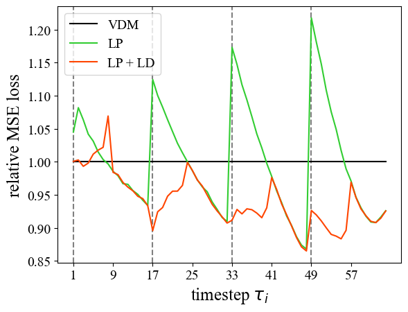
Figure 5: The relative MSE losses of the noise prediction of $\bm{z}_{\tau_{i}}^{i}$ (see Equation 7) when $n=4$. ‘VDM’ indicates original denoising strategy as a reference line. ‘LP’ and ‘LD’ denote latent partitioning and lookahead denoising, respectively.

Although diagonal denoising introduces training-inference gap, it is advantageous in another respect because noisier frames benefit from observing cleaner ones, leading to more accurate denoising. As empirical evidence, Figure 5 shows the relative MSE losses in noise prediction of diagonal denoising with respect to original denoising strategy. The formal definition of the relative MSE is given by

$$\cfrac{||\bm{\epsilon}_{\theta}(\mathbf{z}^{\text{diag}},\bm{\tau}^{\text{diag}})^{i}-\bm{\epsilon}(\mathbf{z}^{\text{vdm}}_{\tau_{i}},\tau_{i}\cdot\bm{1})^{i}||_{2}}{||\bm{\epsilon}_{\theta}(\mathbf{z}^{\text{vdm}}_{\tau_{i}},\tau_{i}\cdot\bm{1})^{i}-\bm{\epsilon}(\mathbf{z}^{\text{vdm}}_{\tau_{i}},\tau_{i}\cdot\bm{1})^{i}||_{2}}.$$ (7)

In the figure, the green graph shows that the predictions of the noisier half are more accurate with diagonal denoising than original denoising strategy. Based on this observation, we propose lookahead denoising to leverage the advantage of diagonal denoising, particularly for the noisier frames in the later half.

As depicted in Figure 4 (b), we utilize the noise estimation for the benefited later half. We perform diagonal denoising with a stride of $f^{\prime}=\lfloor\frac{f}{2}\rfloor$ and update only the later $f^{\prime}$ frames, ensuring that all frames are denoised by refering to a sufficient number—at least $f^{\prime}$—of clearer frames. Precisely, for $k=0,\text{\makebox[5.0pt][c]{.\hfil.\hfil.}\thinspace},2n-1$, each denoising step updates the queue as

$$\text{ {Q}}_{k}^{f^{\prime}+1:f}\leftarrow\Phi(\text{ {Q}}_{k},\bm{\tau}_{k},\bm{c};\epsilon_{\theta})^{f^{\prime}+1:f}.$$ (8)

Algorithm 3 in Appendix C outlines the detailed procedure of FIFO-Diffusion with lookahead denoising. We illustrate the effectiveness of lookahead denoising using the red graph in Figure 5. Except for a few early time steps, the noise prediction with lookahead denoising enhances the denoising capacity of the baseline model, almost completely overcoming the training-inference gap described in Section 4.2. Note that, since we only utilize the half of the model outputs, this approach necessitates twice the computation of diagonal denoising. However, concerns on the computational overhead can be easily handled via parallelization in the same manner as latent partitioning (see Table 1).

5 Experiment

This section presents the videos generated long video generation methods including FIFO-Diffusion, and evaluates them qualitatively and quantitatively. We also perform the ablation study to verify the benefit of latent partitioning and lookahead denoising introduced in FIFO-Diffusion.

5.1 Implementation details

We implement FIFO-Diffusion based on existing open-source text-to-video diffusion models trained on short video clips, including three U-Net based models, VideoCrafter1 (Chen et al., 2023a), VideoCrafter2 (Chen et al., 2024), and zeroscope, as well as a DiT based model, Open-Sora Plan. We employ DDIM sampling (Song et al., 2021a) with $\eta\in\{0.5,1\}$. More details about our implementations can be found in Table 3 in Appendix B.

5.2 Qualitative results

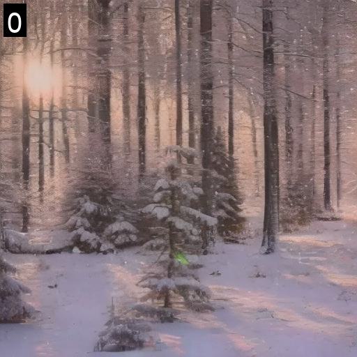
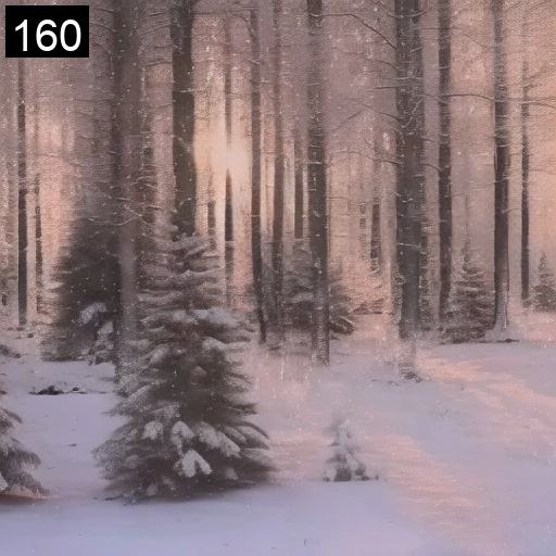
(a) "a serene winter scene in a forest. The forest is blanketed in a thick layer of snow, which . . . "
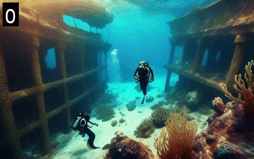
(b) "A vibrant underwater scene of a scuba diver exploring a shipwreck, 2K, photorealistic."
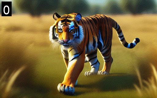
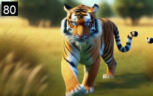
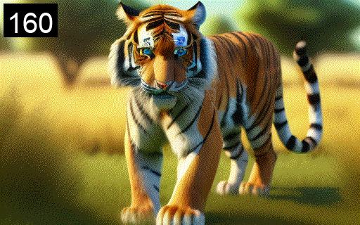
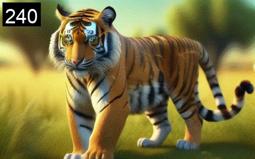
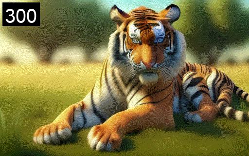
(c) "A tiger walking $\rightarrow$ standing $\rightarrow$ resting on the grassland, photorealistic, 4k, high definition"

Figure 6: Illustrations of long videos generated by FIFO-Diffusion based on (a) Open-Sora Plan and (b) VideoCrafter2, as well as (c) multiple prompts based on VideoCrafter2. The number on the top-left corner of each frame indicates the frame index.

We first evaluate the performance of the proposed approach qualitatively. Figure 1 illustrates examples of extremely long videos (longer than 10K frames) generated by FIFO-Diffusion based on the VideoCrafter2. It demonstrates the ability of FIFO-Diffusion to generate videos of arbitrary lengths, relying solely on the model trained with short video clips. The individual frames exhibit outstanding visual quality with no degradation even in the later part of the videos while semantic information is consistent throughout the videos. Figure 6 (a) and (b) present the generated videos with natural motion of scenes and cameras; the consistency of motion is well-controlled by referencing former frames through the generation process.

Furthermore, Figure 6 (c) shows that FIFO-Diffusion can generate videos including many motions by serially changing prompts. The capability to generate multiple motions and seamless transitions between scenes highlight the practicality of our method. We discuss more details regarding multi-prompts generation in Section E.1. Please refer to Appendices D and E for more examples and our project page1 for video demos, including those based on other baselines.

Ours
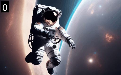
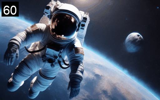
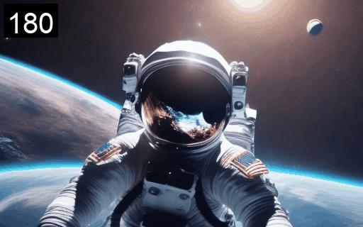
FreeNoise
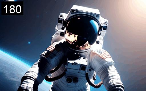
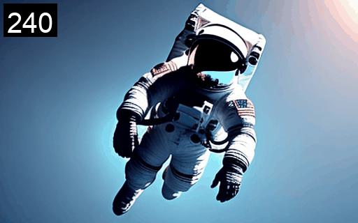
Gen-L-Video
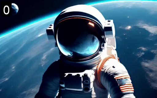
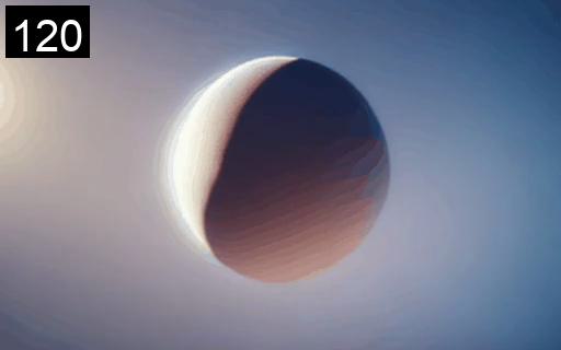
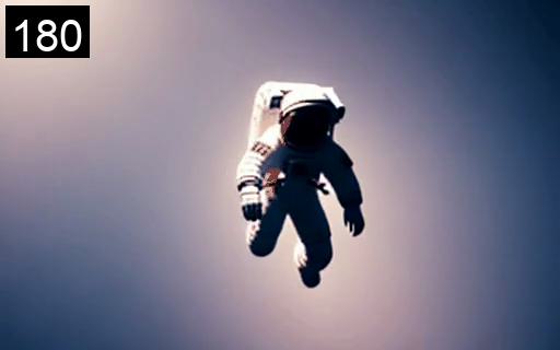
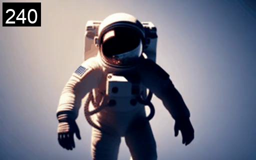
LaVie+SEINE
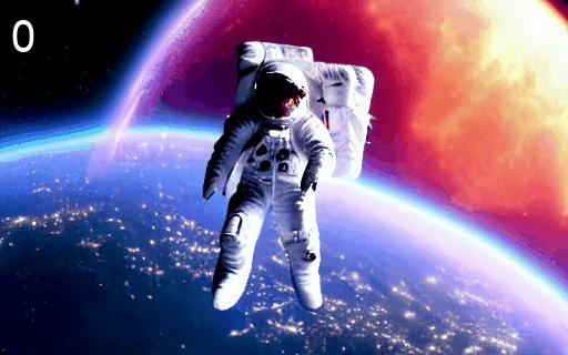
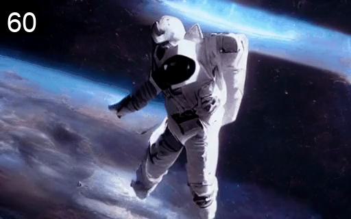
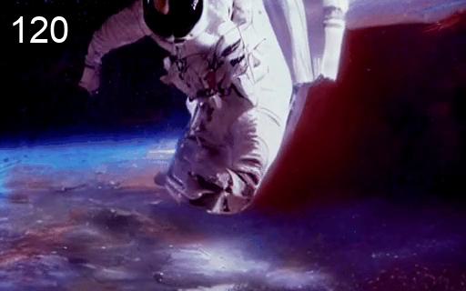
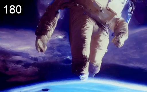
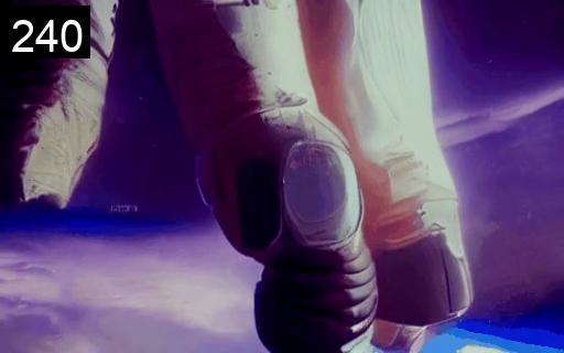
	"An astronaut floating in space, high quality, 4K resolution."

Figure 7: Sample videos generated by (first) FIFO-DIffusion on VideoCrafter2, (second) FreeNoise on VideoCrafter2, (third) Gen-L-Video on VideoCrafter2, and (last) LaVie + SEINE. The number on the top-left corner of each frame indicates the frame index.

In Figure 7, we compare our results with two training-free techniques, FreeNoise (Qiu et al., 2023)and Gen-L-Video (Wang et al., 2023a) applied to VideoCrafter2, as well as a training-based chunked autoregressive method LaVie (Wang et al., 2023c) + SEINE (Chen et al., 2023b). Note that chunked autoregressive method requires two models: LaVie for T2V and SEINE for I2V. We observe that our method significantly outperforms the others in terms of motion smoothness, frame quality, and scene diversity. Among the training-free methods, Gen-L-Video produces blurred background, while FreeNoise fails to generate dynamic scenes and shows a lack of motion. For LaVie + SEINE, their videos gradually degrade and diverge from text due to error accumulation during autoregressive generation. Furthermore, they exhibit periodic discontinuities between chunks, suffering from limited contextual information from the last single frame. More samples are provided in Figures 17 and 18 of Appendix F.

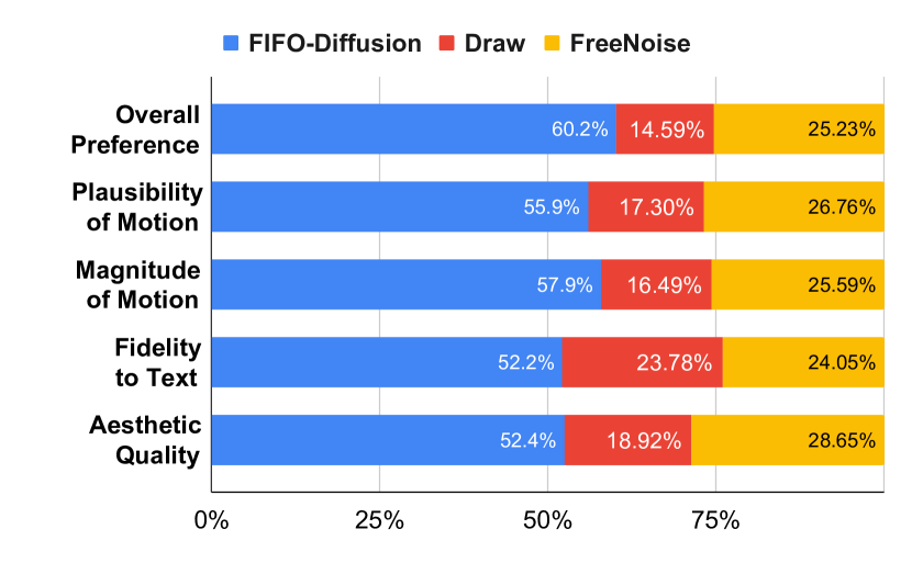
Figure 8: The results of user study between FIFO-Diffusion and FreeNoise for five criteria.

We also conducted a user study to evaluate the performance of FIFO-Diffusion on long video generation in comparison to an existing approach, FreeNoise. Figure 8 shows that the users are substantially favorable to FIFO-Diffusion compared to FreeNoise in all criteria, especially the ones related to motion. Since motion is one of the most distinct properties in videos compared to images, the strong results of FIFO-Diffusion in those criteria are encouraging and show the potential to generate even more natural dynamic videos. The details about the user study are provided in Section B.1.

5.3 Computational cost

We measure memory usage and inference time per frame of training-free long video generation methods including FIFO-Diffusion to analyze scalability and time efficiency. Table 1 shows that FIFO-Diffusion generates videos of arbitrary lengths with a fixed memory allocation, while FreeNoise consumes memory proportional to the target video length. While Gen-L-Video also consumes nearly constant memory, it requires demanding time due to its redundant computation for a frame. Moreover, FIFO-Diffusion can save time with parallelized computation, which is exclusively available for our method. Although incorporating lookahead denoising requires more computation, parallelized inference on multiple GPUs significantly reduces sampling time. For the experiments, we utilize VideoCrafter2 as the baseline model and employ a DDPM scheduler with 64 inference steps on A6000 GPUs.

Table 1: Memory usages and inference times of long video generation methods. ‘LD’ indicates lookahead denosing.

		Memory usage [MB] ($\downarrow$)			Inference time ($\downarrow$) [s/frame]
Method   /   Target # of frames		128	256	512
FreeNoise (Qiu et al., 2023)		26163	44683	OOM	6.09
Gen-L-Video (Wang et al., 2023a)		10913	10937	10965	22.07
FIFO-Diffusion (1 GPU)		11245	11245	11245	6.20
FIFO-Diffusion (4 GPUs)		12210	12210	12210	1.62
FIFO-Diffusion (with LD, 1 GPU)		11245	11245	11245	12.37
FIFO-Diffusion (with LD, 8 GPUs)		13496	13496	13496	1.84

5.4 Ablation study

Table 2: Relative MSE losses of ablations. ‘LP’ and ‘LD’ indicate latent partitioning and lookahead denosing, respectively.

	$n$	without LD	with LD
without LP	1	1.09	1.01
with LP	2	1.04	0.99
with LP	4	1.02	0.98

We conduct ablation study to analyze the effect of latent partitioning and lookahead denoising on the performance of FIFO-Diffusion. Figures 20 and 21 in Appendix H show that latent partitioning significantly improves both quality and temporal consistency of the generated videos, while lookahead denoising further refines videos, making them look natural and smooth by reducing flickering effects.

Additionally, Table 2 compares the relative MSE loss (see Equation 7) averaged over all time steps between ablations. The result shows that latent partitioning effectively reduces the training-inference gap induced by diagonal denoising as the number of partitions increases. Furthermore, lookahead denoising enhances noise prediction accuracy of the model even further, leading to surpass the performance of the original prediction.

5.5 Automated evaluation

We measure FVD (Unterthiner et al., 2018) scores on videos generated with randomly sampled prompts from the MSR-VTT (Xu et al., 2016) test set. For the evaluation of generated long videos, we compute the FVD scores between the 16-frame reference videos obtained from the baseline model and a sequence of the 16-frame windows with a stride 1 of long videos given by FIFO-Diffusion and FreeNoise. We provide further discussion in Appendix G.

6 Limitations

While latent partitioning mitigates the training-inference gap of diagonal denoising and lookahead denoising allows more accurate denoising as shown in Table 2, the gap still remains due to the changes in the model input distribution. However, we believe the benefit of diagonal denoising is also promising for training, and this gap can be resolved by integrating diagonal denoising paradigm into training. We will leave this integration as future work. If the environments for training and inference are aligned, the performance of FIFO-Diffusion can be substantially improved.

7 Conclusion

We presented a novel inference algorithm, FIFO-Diffusion, which allows to generate infinitely long videos from text without tuning video diffusion models pretrained on short video clips. Our method is realized by performing diagonal denoising, which processes latents with increasing noise levels in a first-in-first-out fashion. At each step, a fully denoised instance is dequeued while a new random noise is enqueued. While diagonal denoising has a trade-off, we proposed latent partitioning to alleviate its inherent limitation and lookahead denoising to exploit its strength. Putting them together, FIFO-Diffusion successfully generates long videos with high quality, exhibiting great scene context consistency and dynamic motion expression.

Potential Broader Impact

This paper leverages pretrained video diffusion models to generate high quality videos. The proposed method can potentially be used to synthesize videos with unexpectedly inappropriate content since it is based on pretrained models and involves no training. However, we believe that our method could mildly address ethical concerns associated with the training data of generative models.

Appendix A Details for Lemmas 4.4 and 4.5

A.1 Proof of Lemma 4.4

Lemma 4.4.

If $\bm{\epsilon}(\cdot)$ is bounded, then

$$||\bm{z}_{t}^{i}-\bm{z}_{s}^{i}||=O(|t-s|)~{}~{}\text{for any}~{}~{}i.$$

Proof.

Since $\bm{\epsilon}(\cdot)$ is bounded, there exists some $M>0$ satisfying $||\bm{\epsilon}(\cdot)||\leq M$.

$$||\bm{z}_{t}^{i}-\bm{z}_{s}^{i}|| \leq||\mathbf{z}_{t}^{\text{vdm}}-\mathbf{z}_{s}^{\text{vdm}}||$$

$$=||\int_{s}^{t}c\cdot\bm{\epsilon}(\mathbf{z}_{u}^{\text{vdm}},u\cdot\bm{1})du||$$

$$\leq|\int_{s}^{t}c\cdot||\bm{\epsilon}(\mathbf{z}_{u}^{\text{vdm}},u\cdot\bm{1})||du|$$

$$\leq c\cdot M\cdot|t-s|.$$

∎

A.2 Assumption (H2) of Theorem 4.5

We provide justification for the hypothesis, which the diffusion model is K-Lipschitz continuous. At inference, we can consider $z\in[0,B]^{f\times c\times h\times w}$ and $\sigma\in[\sigma_{\text{min}},\sigma_{\text{max}}]$, where $\sigma_{\text{min}}>0$ since $z$ is pixel values and we inference for such $\sigma$. In appendix B.3 of (Karras et al., 2022), $\epsilon(z,\sigma)$ is given as the following:

$$\epsilon(z,\sigma)=-\sigma\cfrac{\nabla_{z}\sum_{i}\mathcal{N}(z;y_{i},\sigma^{2}\mathbf{I})}{\sum_{i}\mathcal{N}(z;y_{i},\sigma^{2}\mathbf{I})},$$

where ${y_{1},y_{2},\ldots,y_{n}}$ are data points. Note that $\mathcal{N}(z;y_{i},\sigma^{2}\mathbf{I})$ is twice differentiable and continuous, and $\sum_{i}\mathcal{N}(z;y_{i},\sigma^{2}\mathbf{I})\geq c$ for $\exists c>0$. Therefore, the differential function of $\epsilon(z,\sigma)$ is bounded and is Lipschitz continuous. Since $\epsilon_{\theta}(\cdot)$ estimates $\epsilon(\cdot)$, assuming Lipschitz continuity can be justified.

Appendix B Implementation details

We provide the implementation details of the experiments in Table 3. We use VideoCrafter1 (Chen et al., 2023a), VideoCrafter2 (Chen et al., 2024), zeroscope, Open-Sora Plan, LaVie (Wang et al., 2023c), and SEINE (Chen et al., 2023b) as pre-trained models. zeroscope, VideoCrafter, and Open-Sora Plan are under CC BY-NC 4.0, Apache License 2.0, and MIT License, respectively. Except for automated results, all prompts used in experiments are randomly generated by ChatGPT-4 (OpenAI, 2023). We empirically choose $n=4$ for the number of partitions in latent partitioning and lookahead denoising. Also, stochasticity $\eta$, introduced by DDIM (Song et al., 2021a), is chosen to achieve good results from the baseline video generation models.

Table 3: Implementation details regarding experiments

Experiment	Model	$f$	Sampling Method	$n$	$\eta$	# Prompts	# Frames	Resolution
MSE loss	VideoCrafter1	16	FIFO-Diffusion	4	0.5	200	-	$320\times 512$
(Figures 5 and 2)
Qualitative Result	zeroscope	24	FIFO-Diffusion	4	0.5	-	100	$320\times 576$
	VideoCrafter1	16	FIFO-Diffusion	4	0.5	-	100	$320\times 512$
	VideoCrafter2	16	FIFO-Diffusion	4	1	-	100$\sim$10k	$320\times 512$
	Open-Sora Plan	17	FIFO-Diffusion	4	1	-	385	$512\times 512$
	VideoCrafter2	16	FreeNoise	-	1	-	100	$320\times 512$
	VideoCrafter2	16	Gen-L-Video	-	1	-	100	$320\times 512$
	LaVie + SEINE	16	chunked autoregressive	-	1	-	100	$320\times 512$
User Study	VideoCrafter2	16	FIFO-Diffusion	4	1	30	100	$320\times 512$
	LaVie	16	FreeNoise	-	1	30	100	$320\times 512$
Automated Result	VideoCrafter1	16	FIFO-Diffusion	4	0.5	512	100	$256\times 256$
	VideoCrafter1	16	FreeNoise	-	0.5	512	100	$256\times 256$
Ablation study	zeroscope	24	FIFO-Diffusion	$\{1,4\}$	0.5	-	100	$320\times 576$

B.1 Details for user study

We randomly generated 30 prompts from ChatGPT-4 without cherry-picking, and generated a video for each prompt with 100 frames using each method. The evaluators were asked to choose their preference (A is better, draw, or B is better) between the two videos generated by FIFO-Diffusion and FreeNoise with the same prompts, on five criteria: overall preference, plausibility of motion, magnitude of motion, fidelity to text, and aesthetic quality. A total of 70 users submitted 111 sets of ratings, where each set consists of 20 videos from 10 prompts. We used LaVie as the baseline for FreeNoise, since it was the latest model officially implemented at that time.

Appendix C Algorithms of FIFO-Diffusion

This section illustrates pseudo-code for FIFO-Diffusion with and without latent partitioning and lookahead denoising.

Algorithm 1 FIFO-Diffusion with diagonal denoising (Section 4.1)

 $N$, $f$, $\epsilon_{\theta}(\cdot)$, $\text{Dec}(\cdot)$, $\Phi(\cdot)$

Input: $\{\bm{z}_{\tau_{i}}^{i}\}_{i=1}^{f},\{\tau_{i}\}_{i=0}^{f},\bm{c}$

Output: $\bm{v}$

$\bm{v}\leftarrow[]$

$\bm{\tau}\leftarrow[\tau_{1};\text{\makebox[5.0pt][c]{.\hfil.\hfil.}\thinspace};\tau_{f}]$

$\text{ {Q}}\leftarrow[\bm{z}_{\tau_{1}}^{1};\text{\makebox[5.0pt][c]{.\hfil.\hfil.}\thinspace};\bm{z}_{\tau_{f}}^{f}]$

for $i=1$ to $N$ do

     $\text{ {Q}}\leftarrow\Phi(\text{ {Q}},\bm{\tau},\bm{c};\epsilon_{\theta})$ # Equation 3

     $\bm{z}_{\tau_{0}}^{i}\leftarrow\text{ {Q}}\text{.dequeue}()$ # Fully denoised frame

     $\bm{v}\text{.append}(\text{Dec}(\bm{z}_{\tau_{0}}^{i}))$

     $\bm{z}_{\tau_{f}}^{i+f}\sim\mathcal{N}(\mathbf{0},\mathbf{I})$ # New random noise

     $\text{ {Q}}\text{.enqueue}(\bm{z}_{\tau_{f}}^{i+f})$

end for

return $\bm{v}$

Algorithm 2 FIFO-Diffusion with latent partitioning (Section 4.2)

 $N$, $f$, $\epsilon_{\theta}(\cdot),\text{Dec}(\cdot),\Phi(\cdot),n$ # $n\geq 2$ if latent partitioning

Input: $\{\bm{z}_{\tau_{i}}^{i}\}_{i=1}^{nf},\{\tau_{i}\}_{i=0}^{nf},\bm{c}$

Output: $\bm{v}$

$\bm{v}\leftarrow[~{}]$

$\bm{\tau}\leftarrow[\tau_{1};\text{\makebox[5.0pt][c]{.\hfil.\hfil.}\thinspace};\tau_{nf}]$

$\text{ {Q}}\leftarrow[\bm{z}_{\tau_{1}}^{1};\text{\makebox[5.0pt][c]{.\hfil.\hfil.}\thinspace};\bm{z}_{\tau_{nf}}^{nf}]$

for $i=1$ to $N$ do

     for $k=0$ to $n-1$  do# Parallelizable

         $\bm{\tau}_{k}\leftarrow\bm{\tau}^{kf+1:(k+1)f}$

         $\text{ {Q}}_{k}\leftarrow\text{ {Q}}^{kf+1:(k+1)f}$

         $\text{ {Q}}_{k}\leftarrow\Phi(\text{ {Q}}_{k},\bm{\tau}_{k},\bm{c};\epsilon_{\theta})$ # Equation 4

     end for

     $Q\leftarrow[Q_{0};\text{\makebox[5.0pt][c]{.\hfil.\hfil.}\thinspace};Q_{n-1}]$

     $\bm{z}_{\tau_{0}}^{i}\leftarrow\text{ {Q}}\text{.dequeue}()$

     $\bm{v}\text{.append}(\text{Dec}(\bm{z}_{\tau_{0}}^{i}))$

     $\bm{z}_{\tau_{f}}^{i+nf}\sim\mathcal{N}(\mathbf{0},\mathbf{I})$

     $\text{ {Q}}\text{.enqueue}(\bm{z}_{\tau_{nf}}^{i+nf})$

end for

return $\bm{v}$

Algorithm 3 FIFO-Diffusion with lookahead denoising (Section 4.3)

 $N,\epsilon_{\theta}(\cdot),\text{Dec}(\cdot),\Phi(\cdot),n$ # $n\geq 2$ if latent partitioning

Input: $\{\bm{z}_{\tau_{i}}^{i}\}_{i=1}^{nf},\{\tau_{i}\}_{i=0}^{f},\bm{c}$

Output: $\bm{v}$

$\bm{v}\leftarrow[~{}]$

$\bm{\tau}\leftarrow[\overbrace{\tau_{1};\text{\makebox[5.0pt][c]{.\hfil.\hfil.}\thinspace};\tau_{1}}^{f^{\prime}};\tau_{1};\text{\makebox[5.0pt][c]{.\hfil.\hfil.}\thinspace};\tau_{nf}]$

$\text{ {Q}}\leftarrow[\overbrace{\bm{z}_{\tau_{1}}^{1};\text{\makebox[5.0pt][c]{.\hfil.\hfil.}\thinspace};\bm{z}_{\tau_{1}}^{1}}^{f^{\prime}};\bm{z}_{\tau_{1}}^{1};\text{\makebox[5.0pt][c]{.\hfil.\hfil.}\thinspace};\bm{z}_{\tau_{nf}}^{nf}]$ # dummy latents are required

for $i=1$ to $N$ do

     $\bm{z}_{\tau_{1}}^{i}\leftarrow\text{ {Q}}^{f^{\prime}+1}$

     for $k=0$ to $2n-1$  do # Parallelizable

         $\bm{\tau}_{k}\leftarrow\bm{\tau}^{kf^{\prime}+1:(k+2)f^{\prime}}$

         $\text{ {Q}}_{k}\leftarrow\text{ {Q}}^{kf^{\prime}+1:(k+2)f^{\prime}}$

         $\text{ {Q}}_{k}^{f^{\prime}+1:f}\leftarrow\Phi(\text{ {Q}}_{k},\bm{\tau}_{k},\bm{c};\epsilon_{\theta})^{f^{\prime}+1:f}$ # Equation 8

     end for

     $\bm{z}_{\tau_{0}}^{i}\leftarrow\text{ {Q}}_{0}^{f^{\prime}+1}$

     $\bm{v}\text{.append}(\text{Dec}(\bm{z}_{\tau_{0}}^{i}))$

     $\text{ {Q}}_{0}^{f^{\prime}+1}\leftarrow\bm{z}_{\tau_{1}}^{i}$

     $Q\leftarrow[Q_{0}^{1:f^{\prime}};Q_{0}^{f^{\prime}+1:f};\text{\makebox[5.0pt][c]{.\hfil.\hfil.}\thinspace};Q_{2n-1}^{f^{\prime}+1:f}]$

     $Q\leftarrow[Q_{0};Q_{1}^{f^{\prime}+1:f};\text{\makebox[5.0pt][c]{.\hfil.\hfil.}\thinspace};Q_{2n-1}^{f^{\prime}+1:f}]$

      Q.dequeue()

     $\bm{z}_{\tau_{n}f}^{i+nf}\sim\mathcal{N}(\mathbf{0},\mathbf{I})$

     $\text{ {Q}}\text{.enqueue}(\bm{z}_{\tau_{nf}}^{i+nf})$

end for

return $\bm{v}$

Appendix D Qualitative results of FIFO-Diffusion

In Figures 9, 10, 11, 12, 13 and 14, we provide more qualitative results with 4 baselines, VideoCrafter2 (Chen et al., 2024), VideoCrafter1 (Chen et al., 2023a), zeroscope, and Open-Sora Plan.

D.1 VideoCrafter2

(a) "A colony of penguins waddling on an Antarctic ice sheet, 4K, ultra HD."
(b) "A colorful macaw flying in the rainforest, ultra HD."
(c) "A dark knight riding on a black horse on the glassland, photorealistic, 4k, high definition."
(d) "A high-altitude view of a hang glider in flight, high definition, 4K."
(e) "A high-speed motorcycle race on a track, ultra HD, 4K resolution."
(f) "A horse race in full gallop, capturing the speed and excitement, 2K, photorealistic."

Figure 9: Videos generated by FIFO-Diffusion with VideoCrafter2. The number on the top left of each frame indicates the frame index.

(a) "A pair of tango dancers performing in Buenos Aires, 4K, high resolution."
(b) "A panoramic view of a peaceful Zen garden, high-quality, 4K resolution."
(c) "A paraglider soaring over the Alps, photorealistic, 4K, high definition."
(d) "A scenic hot air balloon flight at sunrise, high quality, 4K."
(e) "A scenic hot air balloon flight over Cappadocia, Turkey, 2K, ultra HD."
(f) "A school of colorful fish swimming in a coral reef, ultra high quality, 2K."
(g) "A spectacular fireworks display over Sydney Harbour, 4K, high resolution."

Figure 10: Videos generated by FIFO-Diffusion with VideoCrafter2. The number on the top left of each frame indicates the frame index.

(a) "A spooky haunted house, foggy night, high definition."
(b) "A time-lapse of a busy construction site, high definition, 4K."
(c) "A vibrant underwater scene of a scuba diver exploring a shipwreck, 2K, photorealistic."
(d) "A vibrant, fast-paced salsa dance performance, ultra high quality, 2K."
(e) "An astronaut floating in space, high quality, 4K resolution."
(f) "An astronaut walking on the moon’s surface, high-quality, 4K resolution."
(g) "A majestic lion roaring in the African savanna, ultra HD, 4K."

Figure 11: Videos generated by FIFO-Diffusion with VideoCrafter2. The number on the top left of each frame indicates the frame index.

D.2 VideoCrafter1

(a) "A kayaker navigating through rapids, photorealistic, 4K, high quality."
(b) "A pair of tango dancers performing in Buenos Aires, 4K, high resolution."
(c) "A panoramic view of the Himalayas from a drone, high definition, 4K."
(d) "A paraglider soaring over the Alps, photorealistic, 4K, high definition."
(e) "A professional surfer riding a large wave, high-quality, 4K."
(f) "A school of colorful fish swimming in a coral reef, ultra high quality, 2K."
(g) "An exciting mountain bike trail ride through a forest, 2K, ultra HD."
(h) "A vibrant coral reef with diverse marine life, photorealistic, 2K resolution."

Figure 12: Videos generated by FIFO-Diffusion with VideoCrafter1. The number on the top left of each frame indicates the frame index.

D.3 zeroscope

(a) "A beautiful cherry blossom festival, time-lapse, high quality."
(b) "A close-up of a tarantula walking, high definition."
(c) "A thrilling white water rafting adventure, high definition."
(d) "A detailed macro shot of a blooming rose, 4K."
(e) "A panoramic view of the Milky Way, ultra HD."
(f) "A mysterious foggy forest at dawn, high quality, 4K."
(g) "A scenic cruise ship journey at sunset, ultra HD."
(h) "A lone tree in a vast desert, sunset, high definition."

Figure 13: Videos generated by FIFO-Diffusion with zeroscope. The number on the top left of each frame indicates the frame index.

D.4 Open-Sora Plan

(a) "A quiet beach at dawn, the waves gently lapping at the shore and the sky painted in pastel hues."
(b) "A snowy forest landscape with a dirt road running through it. The road is flanked . . . "
(c) "The majestic beauty of a waterfall cascading down a cliff into a serene lake."
(d) "Slow pan upward of blazing oak fire in an indoor fireplace."
(e) "The dynamic movement of tall, wispy grasses swaying in the wind. The sky above is . . . "
(f) "a serene winter scene in a forest. The forest is blanketed in a thick layer of snow, which . . . "

Figure 14: Videos generated by FIFO-Diffusion with Open-Sora Plan. The number on the top left of each frame indicates the frame index.

Appendix E Multi-prompts generation for FIFO-Diffusion

E.1 Method

For multi-prompts generation, we simply change prompts sequentially during the inference. To be specific, let $\bm{c}_{1},\ldots,\bm{c}_{k}$ be $k$ prompts, and $0=n_{0}<n_{1}<\ldots<n_{k}$ are increasing sequence of integers. Then, we use prompt condition $\bm{c}_{i}$ for $(n_{i-1}+1)^{\text{th}}\sim n_{i}^{\text{th}}$ iterations.

E.2 Qualitative results

In Figures 15 and 16, we provide more qualitative results based on VideoCrafter2.

(a) "Ironman running $\rightarrow$ standing $\rightarrow$ flying on the road, 4K, high resolution."
(b) "A tiger walking $\rightarrow$ standing $\rightarrow$ resting on the grassland, photorealistic, 4k, high definition"
(c) "A teddy bear walking $\rightarrow$ standing $\rightarrow$ dancing on the street, 4K, high resolution."

Figure 15: Videos generated by FIFO-Diffusion with three prompts. The number on the top left of each frame indicates the frame index.

(a) "A tiger resting $\rightarrow$ walking on the grassland, photorealistic, 4k, high definition"
(b) "A whale swimming on the surface of the ocean $\rightarrow$ jumps out of water, 4K, high resolution."
(c) "Titanic sailing through the sunny calm ocean $\rightarrow$ a stormy ocean with lightning, 4K, high resolution."
(d) "A pair of tango dancers performing $\rightarrow$ kissing in Buenos Aires, 4K, high resolution."

Figure 16: Videos generated by FIFO-Diffusion with two prompts. The number on the top left of each frame indicates the frame index.

Appendix F Qualitative comparisons with other long video generation methods

In Figures 17 and 18, we provide more qualitative comparisons with other longer video generation methods, FreeNoise (Qiu et al., 2023), Gen-L-Video (Wang et al., 2023a), and LaVie (Wang et al., 2023c) + SEINE (Chen et al., 2023b).

Ours
FreeNoise
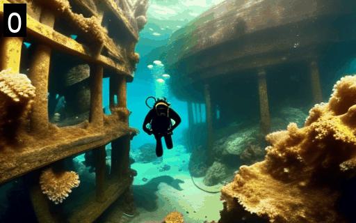
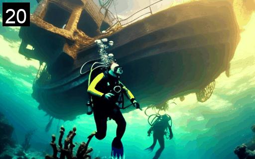
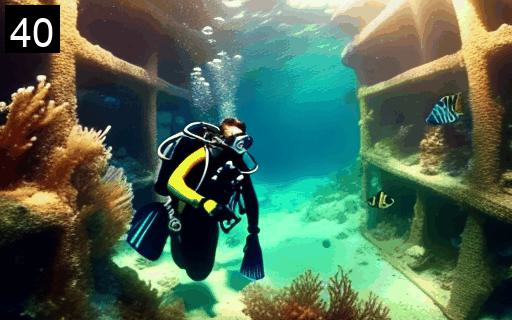
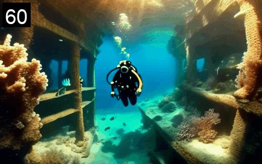
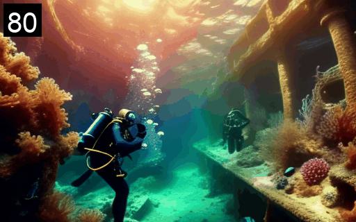
Gen-L-Video
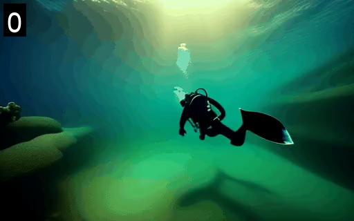
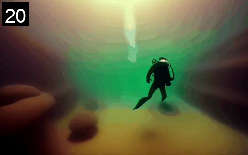
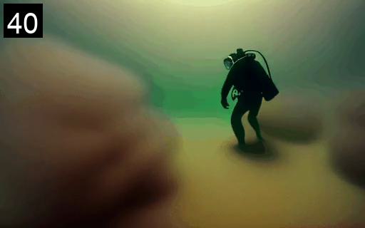
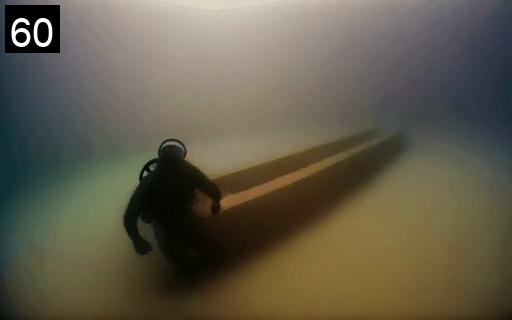
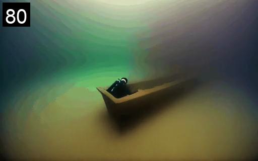
LaVie+SEINE
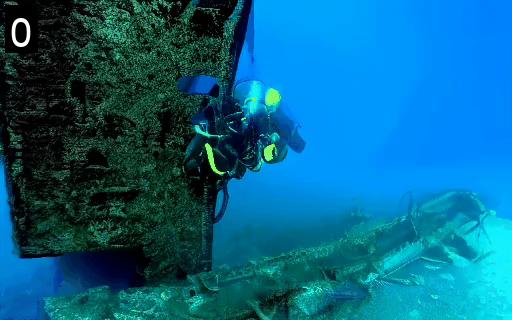
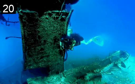
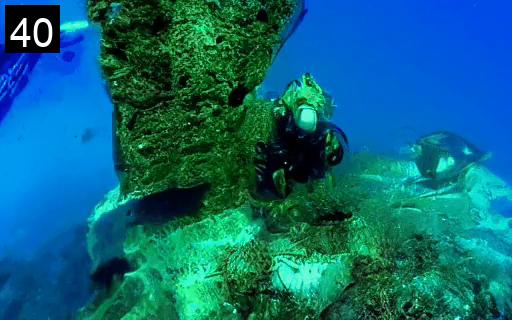
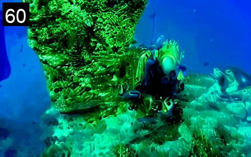
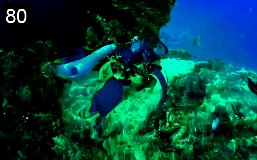
	(a) "A vibrant underwater scene of a scuba diver exploring a shipwreck, 2K, photorealistic."
Ours
FreeNoise
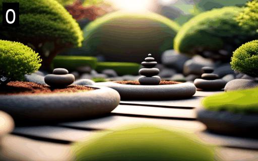
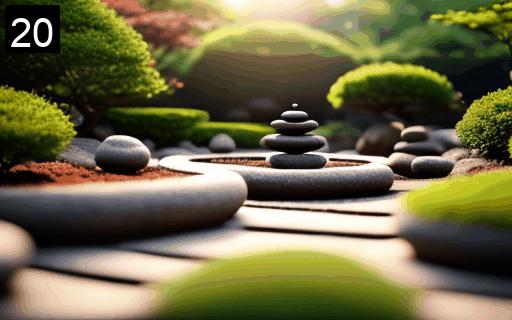
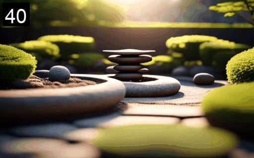
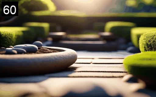
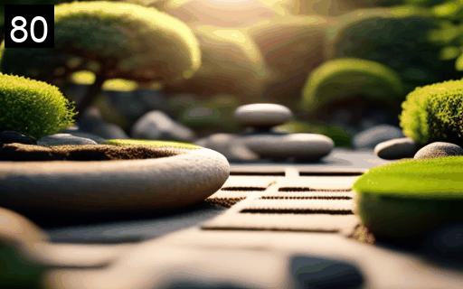
Gen-L-Video
LaVie+SEINE
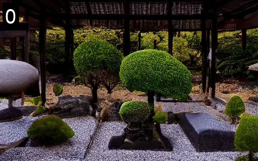
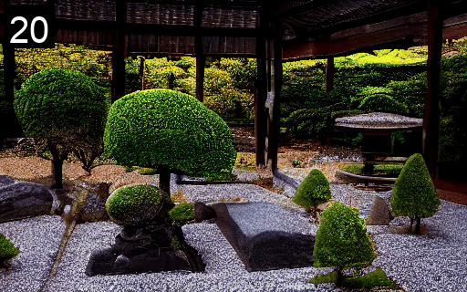
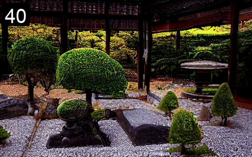
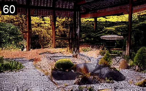
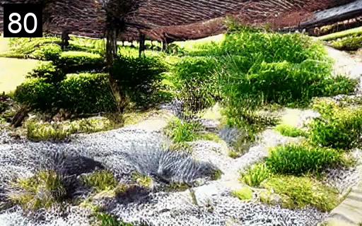
	(b) "A panoramic view of a peaceful Zen garden, high-quality, 4K resolution."

Figure 17: Qualitative comparisons with other long video generation techniques, Gen-L-Video, FreeNoise, and LaVie + SEINE. The number in the top-left corner of each frame indicates the frame index.

Ours
FreeNoise
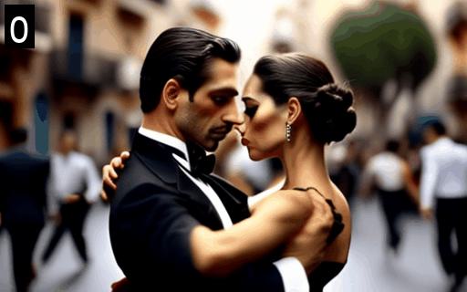
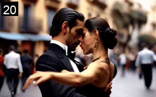
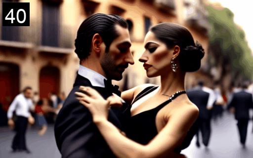
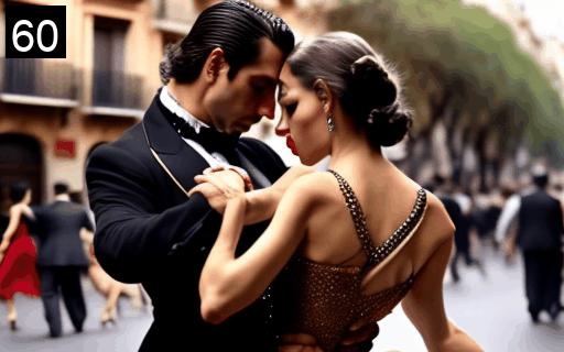
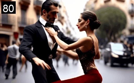
Gen-L-Video
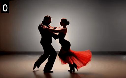
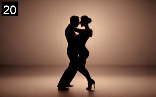
LaVie+SEINE
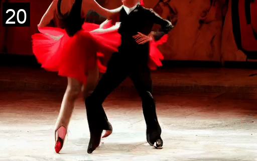
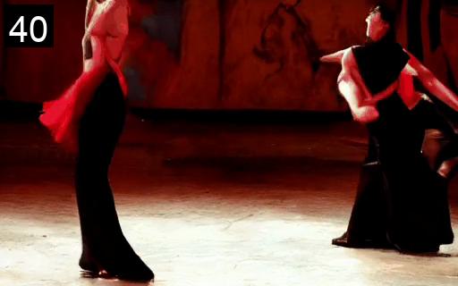
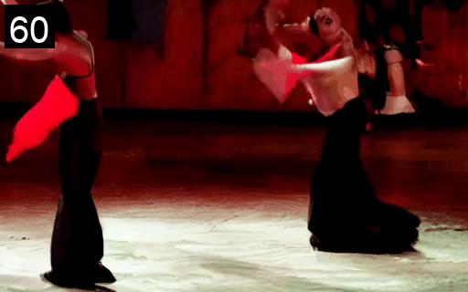
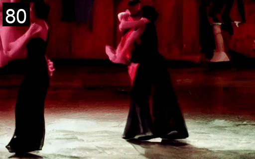
	(a) "A pair of tango dancers performing in Buenos Aires, 4K, high resolution."
Ours
FreeNoise
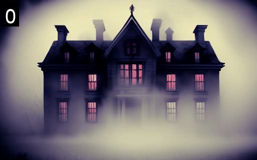
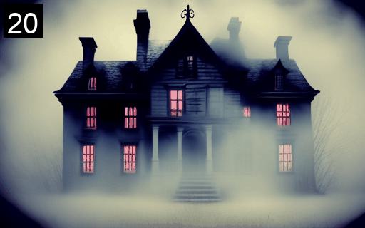
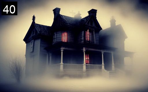
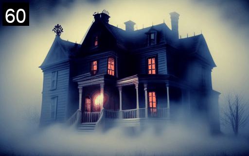
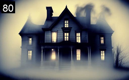
Gen-L-Video
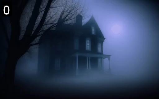
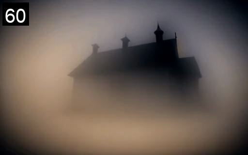
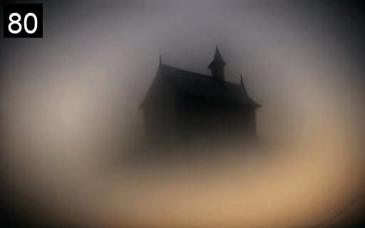
LaVie+SEINE
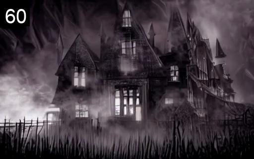
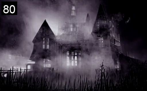
	(b) "A spooky haunted house, foggy night, high definition."

Figure 18: Qualitative comparisons with other long video generation techniques, Gen-L-Video, FreeNoise, and LaVie + SEINE. The number in the top-left corner of each frame indicates the frame index.

Appendix G Automated evaluation

Figure 19 shows that the FVD scores of FIFO-Diffusion are generally higher than those of FreeNoise (Qiu et al., 2023), especially in the later parts of the videos. The rapidly increasing trend in the early frames of FIFO-Diffusion is partly due to the fact that it starts with the corrupted latents generated by the baseline model, as described in Section 4.2. However, we consider these quantitative results to be weak criteria for comparing algorithms. This is because, as the recent study (Girdhar et al., 2023) points out, the automated metrics for videos are often poorly correlated with human perception and insensitive to the quality of generated videos; FVD is more favorable to the algorithms that generate nearly static videos due to the feature similarity to the reference frames.

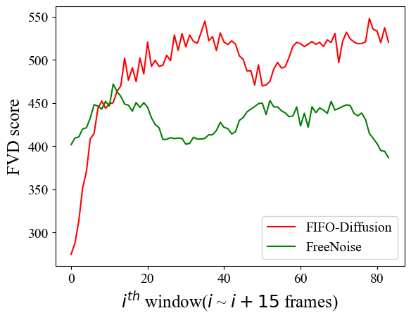
Figure 19: FVD scores of FIFO-Diffusion and FreeNoise with respect to the reference video generated by the baseline

Appendix H Ablation study

In Figures 20 and 21, we conduct an ablation study to investigate the effectiveness of each component in FIFO-Diffusion. We compare the results of FIFO-Diffusion only with diagonal denoising (DD), with the addition of latent partitioning with n=4 (DD + LP), and lookahead denoising (DD + LP + LD).

DD
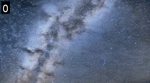
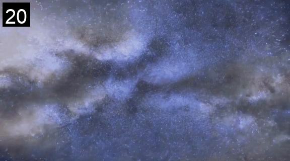
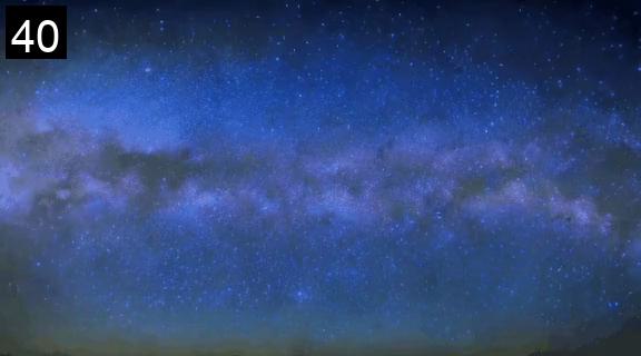
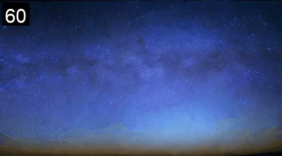
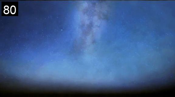
DD+LP
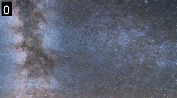
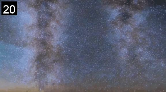
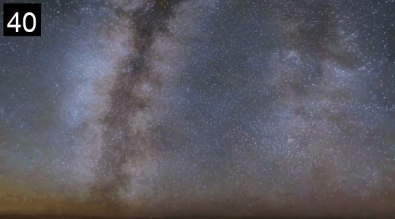
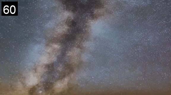
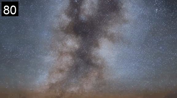
DD+LP+LD
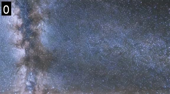
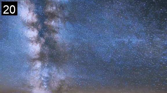
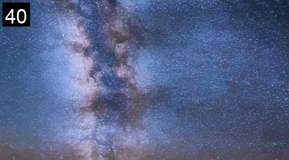
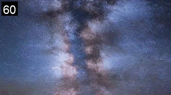
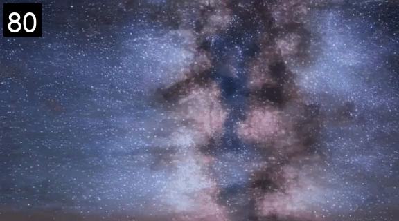
	(a) "A panoramic view of the Milky Way, ultra HD."
DD
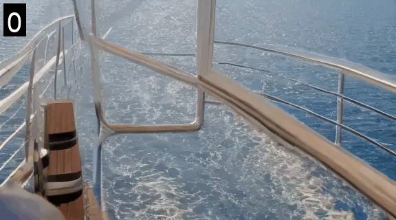
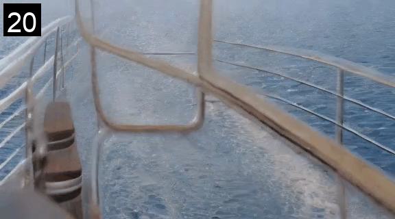
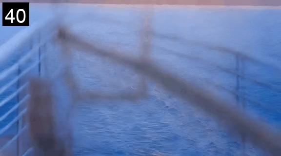
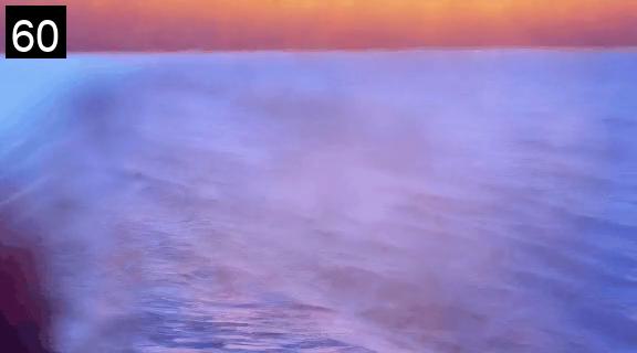
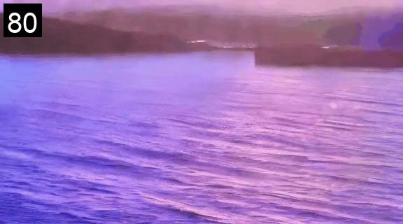
DD+LP
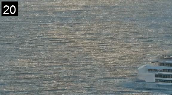
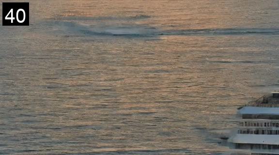
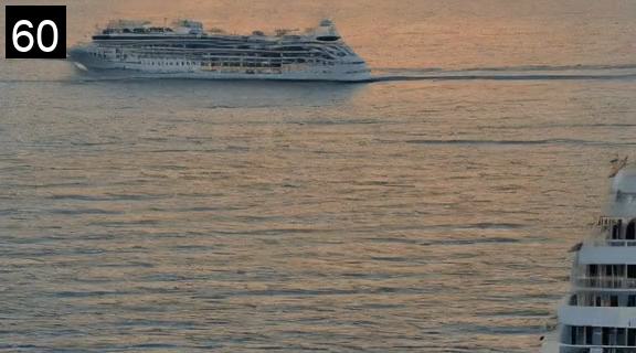
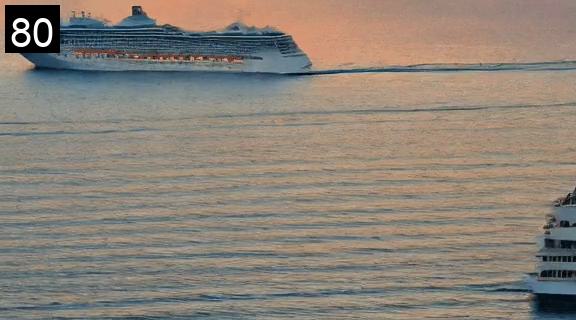
DD+LP+LD
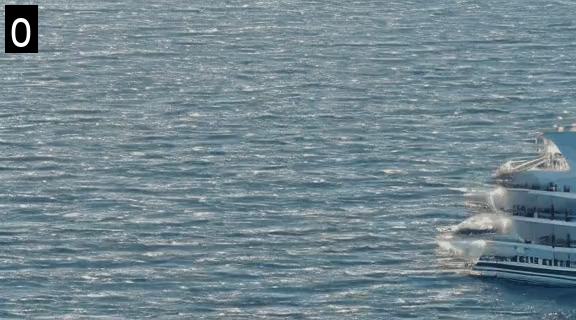
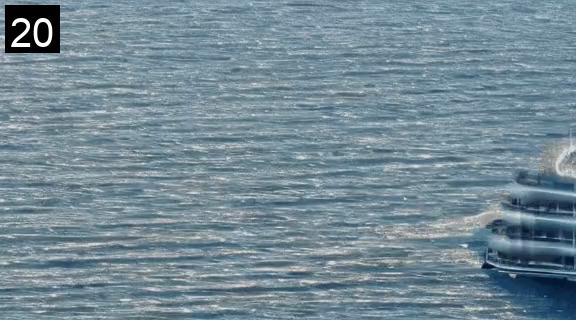
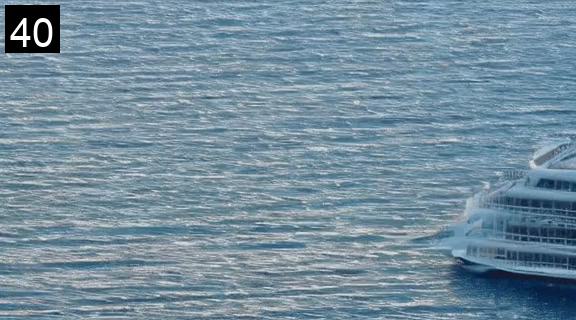
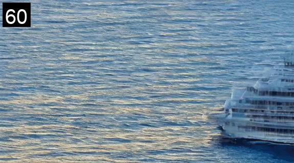
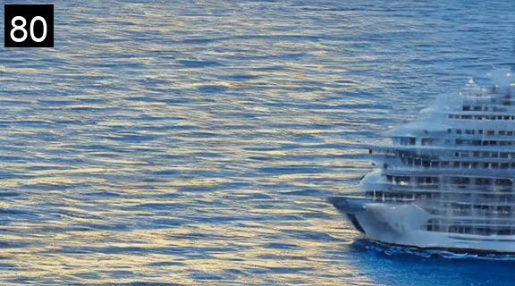
	(b) "A scenic cruise ship journey at sunset, ultra HD."
DD
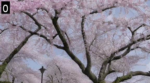
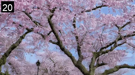
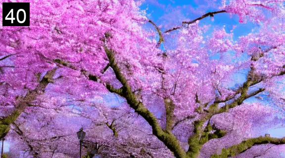
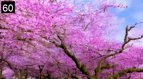
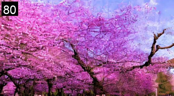
DD+LP
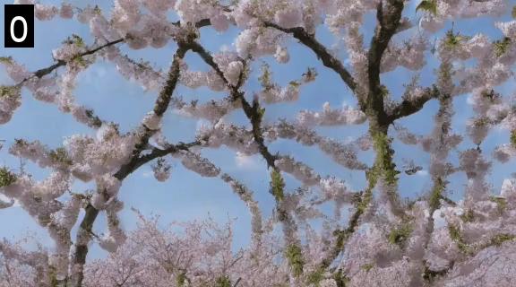
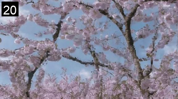
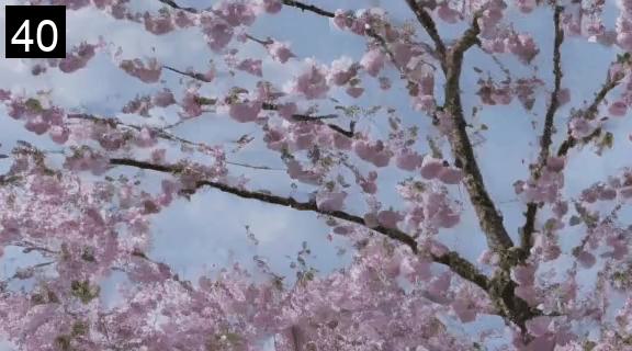
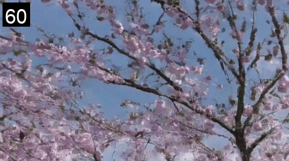
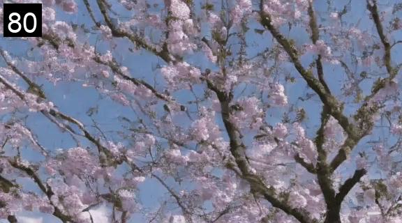
DD+LP+LD
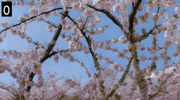
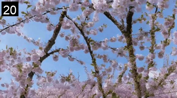
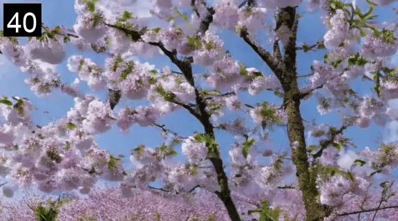
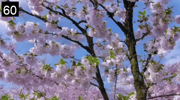
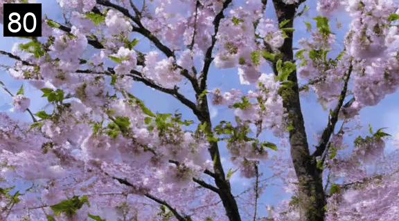
	(c) "A beautiful cherry blossom festival, time-lapse, high quality."

Figure 20: Ablation study. DD, LP, and LD signifies diagonal denoising, latent partitioning, and lookahead denoising, respectively. The number on the top-left corner of each frame indicates the frame index.

DD
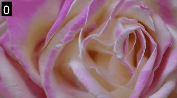
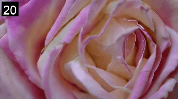
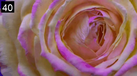
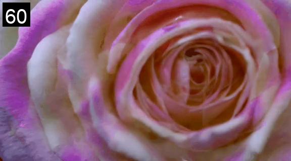
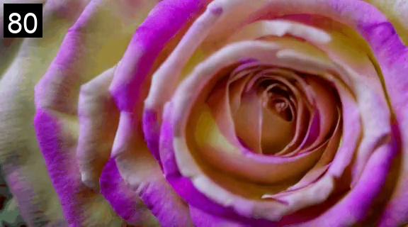
DD+LP
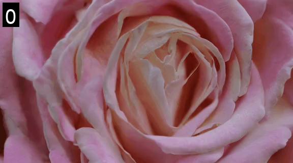
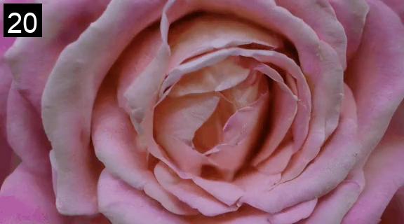
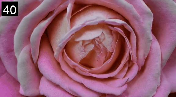
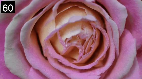
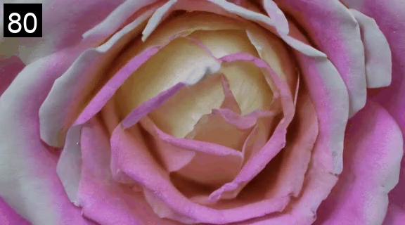
DD+LP+LD
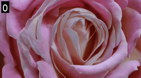
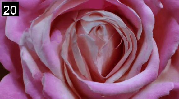
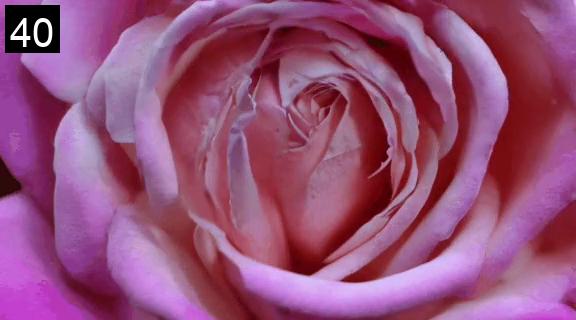
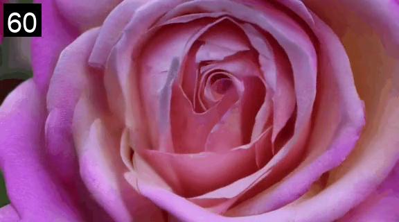
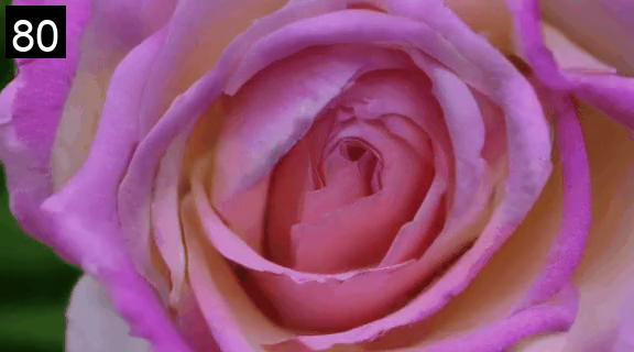
	(a) "A detailed macro shot of a blooming rose, 4K."
DD
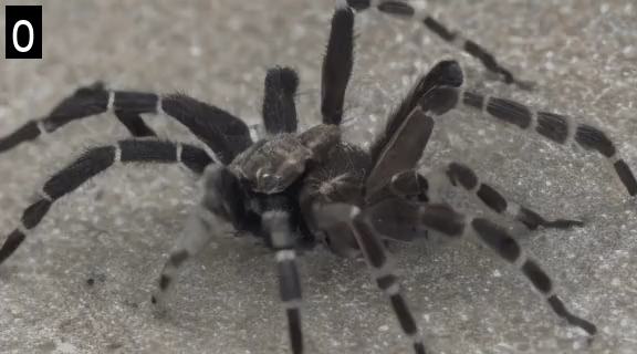
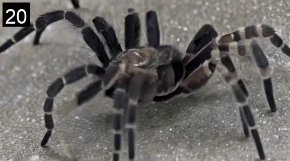
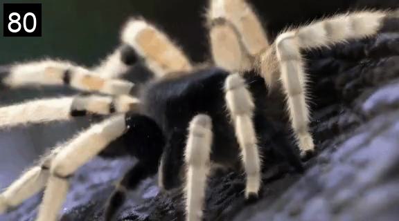
DD+LP
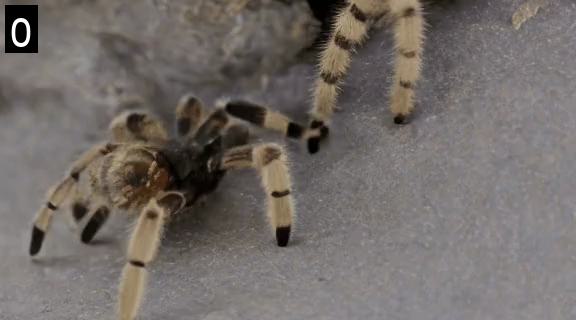
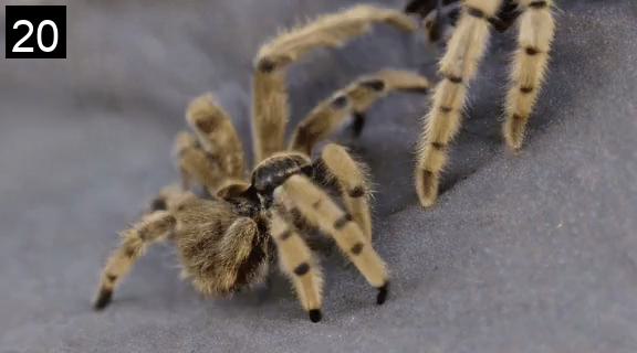
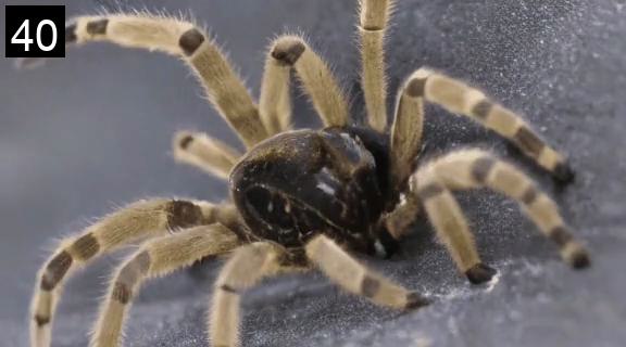
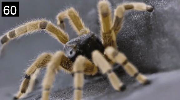
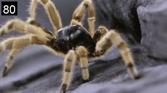
DD+LP+LD
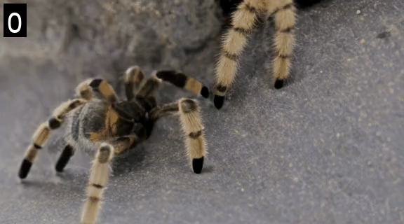
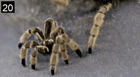
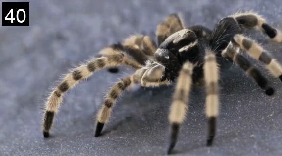
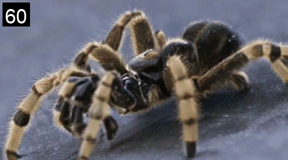
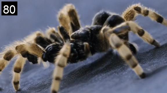
	(b) "A close-up of a tarantula walking, high definition."

Figure 21: Ablation study. DD, LP, and LD signifies diagonal denoising, latent partitioning, and lookahead denoising, respectively. The number on the top-left corner of each frame indicates the frame index.

References

- Blattmann et al. (2023) Blattmann, A., Rombach, R., Ling, H., Dockhorn, T., Kim, S. W., Fidler, S., and Kreis, K. Align your latents: High-resolution video synthesis with latent diffusion models. In CVPR, 2023.
- Chen et al. (2023a) Chen, H., Xia, M., He, Y., Zhang, Y., Cun, X., Yang, S., Xing, J., Liu, Y., Chen, Q., Wang, X., Weng, C., and Shan, Y. VideoCrafter1: Open diffusion models for high-quality video generation. arXiv preprint arXiv:2310.19512, 2023a.
- Chen et al. (2024) Chen, H., Zhang, Y., Cun, X., Xia, M., Wang, X., Weng, C., and Shan, Y. VideoCrafter2: Overcoming data limitations for high-quality video diffusion models. arXiv preprint arXiv:2401.09047, 2024.
- Chen et al. (2023b) Chen, X., Wang, Y., Zhang, L., Zhuang, S., Ma, X., Yu, J., Wang, Y., Lin, D., Qiao, Y., and Liu, Z. Seine: Short-to-long video diffusion model for generative transition and prediction. arXiv preprint arXiv:2310.20700, 2023b.
- Dhariwal & Nichol (2021) Dhariwal, P. and Nichol, A. Diffusion models beat GANs on image synthesis. In NeurIPS, 2021.
- Girdhar et al. (2023) Girdhar, R., Singh, M., Brown, A., Duval, Q., Azadi, S., Rambhatla, S. S., Shah, A., Yin, X., Parikh, D., and Misra, I. Emu video: Factorizing text-to-video generation by explicit image conditioning. arXiv preprint arXiv:2311.10709, 2023.
- Harvey et al. (2022) Harvey, W., Naderiparizi, S., Masrani, V., Weilbach, C., and Wood, F. Flexible diffusion modeling of long videos. In NeurIPS, 2022.
- He et al. (2022) He, Y., Yang, T., Zhang, Y., Shan, Y., and Chen, Q. Latent video diffusion models for high-fidelity long video generation. arXiv preprint arXiv:2211.13221, 2022.
- Ho et al. (2020) Ho, J., Jain, A., and Abbeel, P. Denoising diffusion probabilistic models. In NeurIPS, 2020.
- Ho et al. (2022) Ho, J., Salimans, T., Gritsenko, A., Chan, W., Norouzi, M., and Fleet, D. J. Video diffusion models. In NeurIPS, 2022.
- Hong et al. (2023) Hong, W., Ding, M., Zheng, W., Liu, X., and Tang, J. CogVideo: Large-scale pretraining for text-to-video generation via transformers. In ICLR, 2023.
- Karras et al. (2022) Karras, T., Aittala, M., Aila, T., and Laine, S. Elucidating the design space of diffusion-based generative models. In NeurIPS, 2022.
- Luo et al. (2023) Luo, Z., Chen, D., Zhang, Y., Huang, Y., Wang, L., Shen, Y., Zhao, D., Zhou, J., and Tan, T. Videofusion: Decomposed diffusion models for high-quality video generation. In CVPR, 2023.
- OpenAI (2023) OpenAI. GPT-4 technical report. arXiv preprint arXiv:2303.08774, 2023.
- Peebles & Xie (2023) Peebles, W. and Xie, S. Scalable diffusion models with transformers. In ICCV, 2023.
- Qiu et al. (2023) Qiu, H., Xia, M., Zhang, Y., He, Y., Wang, X., Shan, Y., and Liu, Z. FreeNoise: Tuning-free longer video diffusion via noise rescheduling. arXiv preprint arXiv:2310.15169, 2023.
- Rombach et al. (2022) Rombach, R., Blattmann, A., Lorenz, D., Esser, P., and Ommer, B. High-resolution image synthesis with latent diffusion models. In CVPR, 2022.
- Ronneberger et al. (2015) Ronneberger, O., Fischer, P., and Brox, T. U-Net: Convolutional networks for biomedical image segmentation. In MICCAI, 2015.
- Singer et al. (2022) Singer, U., Polyak, A., Hayes, T., Yin, X., An, J., Zhang, S., Hu, Q., Yang, H., Ashual, O., Gafni, O., Parikh, D., Gupta, S., and Taigman, Y. Make-A-Video: Text-to-video generation without text-video data. In ICLR, 2022.
- Song et al. (2021a) Song, J., Meng, C., and Ermon, S. Denoising diffusion implicit models. In ICLR, 2021a.
- Song et al. (2021b) Song, Y., Sohl-Dickstein, J., Kingma, D. P., Kumar, A., Ermon, S., and Poole, B. Score-based generative modeling through stochastic differential equations. In ICLR, 2021b.
- Unterthiner et al. (2018) Unterthiner, T., van Steenkiste, S., Kurach, K., Marinier, R., Michalski, M., and Gelly, S. Towards accurate generative models of video: A new metric & challenges. arXiv preprint arXiv:1812.0171, 2018.
- Villegas et al. (2023) Villegas, R., Babaeizadeh, M., Kindermans, P.-J., Moraldo, H., Zhang, H., Saffar, M. T., Castro, S., Kunze, J., and Erhan, D. Phenaki: Variable length video generation from open domain textual description. In ICLR, 2023.
- Voleti et al. (2022) Voleti, V., Jolicoeur-Martineau, A., and Pal, C. MCVD: Masked conditional video diffusion for prediction, generation, and interpolation. In NeurIPS, 2022.
- Wang et al. (2023a) Wang, F.-Y., Chen, W., Song, G., Ye, H.-J., Liu, Y., and Li, H. Gen-L-Video: Multi-text to long video generation via temporal co-denoising. arXiv preprint arXiv:2305.18264, 2023a.
- Wang et al. (2023b) Wang, J., Yuan, H., Chen, D., Zhang, Y., Wang, X., and Zhang, S. ModelScope text-to-video technical report. arXiv preprint arXiv:2308.06571, 2023b.
- Wang et al. (2023c) Wang, Y., Chen, X., Ma, X., Zhou, S., Huang, Z., Wang, Y., Yang, C., He, Y., Yu, J., Yang, P., Guo, Y., Wu, T., Si, C., Jiang, Y., Chen, C., Loy, C. C., Dai, B., Lin, D., Qiao, Y., and Liu, Z. LaVie: High-quality video generation with cascaded latent diffusion models. arXiv preprint arXiv:2309.15103, 2023c.
- Xu et al. (2016) Xu, J., Mei, T., Yao, T., and Rui, Y. MSR-VTT: A large video description dataset for bridging video and language. In CVPR, 2016.
- Yang et al. (2023) Yang, S., Zhang, L., Liu, Y., Jiang, Z., and He, Y. Video diffusion models with local-global context guidance. In IJCAI, 2023.
- Yin et al. (2023) Yin, S., Wu, C., Yang, H., Wang, J., Wang, X., Ni, M., Yang, Z., Li, L., Liu, S., Yang, F., Fu, J., Ming, G., Wang, L., Liu, Z., Li, H., and Duan, N. NUWA-XL: Diffusion over diffusion for extremely long video generation. arXiv preprint arXiv:2303.12346, 2023.
- Zhou et al. (2022) Zhou, D., Wang, W., Yan, H., Lv, W., Zhu, Y., and Feng, J. MagicVideo: Efficient video generation with latent diffusion models. arXiv preprint arXiv:2211.11018, 2022.