Control-Aware Transmit Power Allocation for 6G In-Factory Subnetwork Control Systems

Abstract

In this paper, we develop a novel power control solution for subnetworks-enabled distributed control systems in factory settings. We propose a channel-independent control-aware (CICA) policy based on the logistic model and learn the parameters using Bayesian optimization with a multi-objective tree-structured Parzen estimator. The objective is to minimize the control cost of the plants, measured as a finite horizon linear quadratic regulator cost. The proposed policy can be executed in a fully distributed manner and does not require cumbersome measurement of channel gain information, hence it is scalable for large-scale deployment of subnetworks for distributed control applications. With extensive numerical simulation and considering different densities of subnetworks, we show that the proposed method can achieve competitive stability performance and high availability for large-scale distributed control plants with limited radio resources.

I Introduction

The modularity vision of the future industrial revolution necessitates the replacement of rigid communication wirelines with reliable wireless connections even at the field level [1]. This is an objective that 6G aims to achieve in the context of in-X subnetworks, located at the edge of the 6G network of network architecture[2, 3]. Subnetworks are short-range cells that can be installed in a robot or production module to provide reliable local communication between wireless sensors/actuators and the controller for autonomous control operations. Given the potentially high number of autonomous robots and production modules on a factory floor, subnetworks can become very dense resulting in cumbersome interference. Efficient radio resource management techniques like transmit power control (PC) are essential to mitigate the resulting interference and ensure the stability of the controlled plants.

In the framework of 6G in-X subnetworks, novel RRM algorithms are being studied for interference coordination [3, 4, 5, 6] including heuristics [4] and machine learning solutions [5, 6]. The PC problem for in-factory subnetworks was investigated in [6], where the authors propose a graph neural network-based algorithm with scalable sensing and signalling complexity considering subnetworks’ large scale and density. The proposed methods in [4, 5, 6] are based on communication metrics, such as a minimum required transmission rate. However, the goal of controlling a plant is to ensure plant stability. Hence, objectives based on communication requirements but unaware of the control objective may lead to over-provisioning and improper allocation of limited radio resources [7].

This paper addresses this limitation by incorporating control awareness in transmit power optimization for dense subnetworks deployed for closed-loop control operations. The potential benefit of considering control awareness in RRM has been demonstrated in [8, 9, 10, 11, 12]. These studies considered scheduling problems in a wireless network control system (WNCS) architecture that includes multiple plants connected to a centralized controller/base station via a shared wireless medium. They show that the control-aware scheduling policy generally outperforms the control-agnostic scheduling policy in ensuring the stability of the control plants with higher radio resource efficiency.

The concept of In-Factory Subnetwork Control Systems (InF-SCS) encompasses multiple subnetworks simultaneously operating on the same floor, where each subnetwork carries a controller co-located with an access point (AP) to support one or more plants as in Fig. 1. This concept differs from the WNCS architecture studied in [8, 9, 10, 11, 12], where the authors focused on solving scheduling problems for single radio cells serving multiple plants. The closest reference to our work is [12]. The authors consider PC for multiple plants organized in a multicellular architecture. They propose a reinforcement learning algorithm that uses observation of the instantaneous channel gain of all the interfering and desired communication links. However, the sensing and signalling complexity required to collect such observation does not scale to the high density and large scale of InF-SCS [6].

In this study, our goal is to efficiently coordinate interference in large-scale and dense InF-SCS settings using the stability information of the associated control plants, without the need for cumbersome radio channel gain measurements. Our major contributions are $(1)$ We model the transmit power optimization problem for InF-SCS to minimize the control costs of the associated plants with limited radio resources. $(2)$ We propose a simple channel-independent control-aware (CICA) PC algorithm based on a logistic model. $(3)$ We adopt a Bayesian optimization (BO) method using a multi-objective tree-structured Parzen estimator (MOTPE) to learn the parameters of the CICA model. $(4)$ We conduct extensive numerical simulations to compare the performance of our proposed model to several benchmark algorithms.

The paper is structured as follows. In the next section, we present the system model of the InF-SCS. The optimization problem and the proposed solution are discussed in Section III. Simulation assumptions and results are shown in Section IV. Finally, conclusions and an outlook towards future work are presented in Section V.

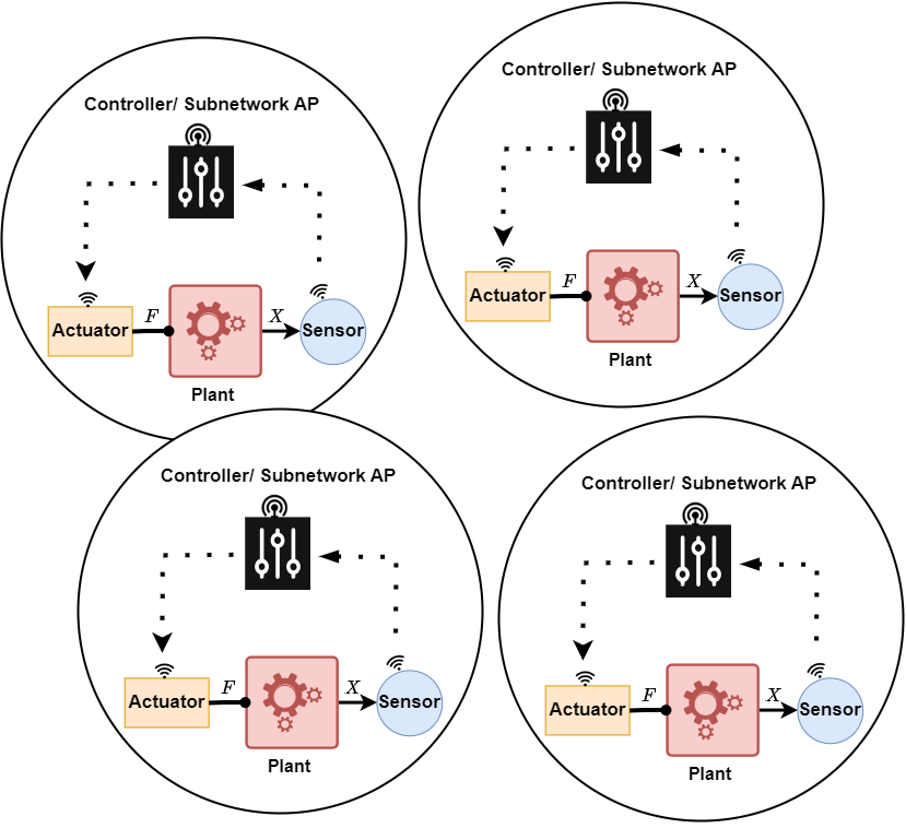
Figure 1: In-Factory Subnetwork Control Systems (InF-SCS) supporting closed-loop control of distributed plants.

II In-Factory Subnetwork Control System Model

An InF-SCS consists of a group of short-range subnetworks providing wireless connectivity for control plants as illustrated in Fig. 1. The controller is co-located with the AP in a subnetwork associated with one or more plants. The controller receives the state from the sensors in the uplink and generates a control signal based on a control objective. The controller then sends the control signal to the actuators in the downlink to complete the closed-loop operation. We consider $N$ independent subnetworks, each supporting a single plant. We index the subnetworks and corresponding plants by $n={1,2,\cdots,N}$. The stability of the control system supported by the subnetworks depends on the plants’ specifications and the delays in communication. Such delays depend on the achievable transmission rate, a function of the transmission bandwidth, power and interference levels. We assume that uplink and downlink transmissions occur over different frequency bands. The downlink transmission of the control signal from the controller to the actuator occurs at every successful reception of the plant state data. The control signal is generally considered relatively small, e.g., a few tens of bytes compared to the sensor data that could be as high as tens of megabytes [8, 13]. Hence, we assume the control signal can always be delivered without PC, and we focus on PC for the uplink communication between the sensor and the controller in the subnetwork, which poses the main limitation to closing the control loop. We consider discrete linear time-invariant (LTI) plants. The state vector $\mathbf{x}^{(t+1)}_{n}\in\mathbb{R}^{q}$ of the plant $n$ due to control action vector $\mathbf{u}^{(t)}_{n}\in\mathbb{R}^{r}$ at time $t$ is given by [11, 8]

$$\mathbf{x}^{(t+1)}_{n}=\mathbf{A}_{n}\mathbf{x}^{(t)}_{n}+\mathbf{B}_{n}\mathbf{u}^{(t)}_{n}+\mathbf{w}_{n}^{(t)},$$ (1)

where $q$ is the number of state variables and $r$ is the number of control action variables. The system dynamics is defined by the state transition matrices $\mathbf{A}_{n}\in\mathbb{R}^{q\times q}$ and $\mathbf{B}_{n}\in\mathbb{R}^{q\times r}$. $\mathbf{A}_{n}$ dictates how the state vector of the system changes from $t$ to $t+1$ when no control action is applied. $\mathbf{B}_{n}$ expresses how the state of the system changes from $t$ to $t+1$ when control action $\mathbf{u}^{(t)}_{n}$ is applied. $\mathbf{w}^{(t)}_{n}\in\mathbb{R}^{q}$ is the Gaussian noise with zero mean and covariance $\mathbf{\Sigma}_{n}$. We assume that even with no action, $\mathbf{x}^{(t)}_{n}\to\infty\text{ as }t\to\infty$, i.e. $\mathbf{A}_{n}$ is unstable. If the plant state information is not available, the plant operates in an open loop, using a local estimate of the control action $\mathbf{\tilde{u}}_{n}^{(t)}$ as in (2). We assume $\mathbf{\tilde{u}}_{n}^{(t)}=\mathbf{u}_{n}^{t-1}$ .

$$\mathbf{u}_{n}^{(t)}=\begin{cases}-\mathbf{\varphi}\tilde{\mathbf{x}}_{n}^{(t)},\ \text{closed loop}\\ \mathbf{\tilde{u}}_{n}^{(t)},\ \text{open loop}\end{cases}$$ (2)

$$\tilde{\mathbf{x}}_{n}^{(t)}=\mathbf{x}_{n}^{(t-t_{D})}+\mathbf{w}_{n}^{(t)}.$$ (3)

Where $t_{D}$ is the time delay introduced by the uplink communication in delivering a piece of state information that was generated in time $t-t_{D}$. $t_{D}$ is a function of the rate and the data size. $\mathbf{\varphi}$ is the optimal control policy gain derived by solving the algebraic Riccati equation (ARE)[14]. The solution to ARE is the optimal control policy that minimizes the cost function [14, 8], i.e.

$$J(\mathbf{x}_{n},\mathbf{u}_{n})=\int_{0}^{\infty}(\mathbf{x}_{n}^{T}\mathbf{Q}_{n}\mathbf{x}_{n}+\mathbf{u}_{n}^{T}\mathbf{R}_{n}\mathbf{u}_{n})dt.$$ (4)

$J(\mathbf{x}_{n},\mathbf{u}_{n})$ is popularly referred to as the infinite horizon linear quadratic regulator (LQR) cost. $\mathbf{Q}_{n}\in\mathbb{R}^{q\times q}$ is the state cost matrix which weighs the relative importance of each state variable in the state vector. $\mathbf{R}_{n}\in\mathbb{R}^{r\times r}$ is the input action cost matrix which penalizes the actuator effort. The plant’s stability can be monitored by an estimate of (4) over an infinite horizon.

For brevity, we assume that the sensors associated with the plant are co-located with a single wireless transmitter and the actuators are co-located with a single wireless receiver. A fresh packet of the state information $\mathbf{x}^{(t)}_{n}$ of size $D_{n}$ (bits) is added in the sensor transmitter buffer periodically every $T_{n}$ (ms). The buffer is considered to have a size of $L_{n}$ to store successive sensor information. At transmission time interval (TTI) $\delta t$, the sensor transmitter in subnetwork $n$ transmits the amount of bits corresponding to its achievable rate at time $t$ given by the Shannon approximation,

$$\Upsilon_{n}^{(t)}(\mathbf{p}^{(t)},\mathbf{\Gamma}^{(t)})=B\log_{2}\left(1+\frac{p_{n}^{(t)}\mid\gamma_{n}^{(t)}\mid^{2}}{\sum\limits_{\begin{subarray}{c}m\in\mathcal{N}^{(t)}\\ m\neq n\end{subarray}}p_{m}^{(t)}\mid\gamma_{m,n}^{(t)}\mid^{2}+\sigma^{2}}\right)$$ (5)

in (bits/s) to its controller/AP. where $\gamma^{(t)}_{n}$ is the desired link channel gain with transmit power, $p_{n}^{(t)}\coloneqq(\mathbf{p}^{(t)})_{n}\in\mathbb{R}^{N}$. All the transmitters reuse the same frequency with bandwidth $B$ ($\rm{Hz}$). $\gamma_{m,n}^{t}\coloneqq(\mathbf{\Gamma}^{(t)})_{m,n}\in\mathbb{C}^{N\times N}$ represents the channel gain of the interfering transmitter in subnetwork $m\neq n$ at time $t$ transmitting with power $p_{m}^{(t)}\coloneqq(\mathbf{p}^{(t)})_{m}$. $\sigma^{2}=\mathcal{J}TB\cdot 10^{NF/10}$ is the thermal noise power with $\mathcal{J}$ being the Boltzmann constant, $NF$ represents the Noise figure ($\rm{dB}$), and $T$ is the temperature (Kelvin). $\mathcal{N}^{(t)}$ represents the set of subnetworks transmitting at time t. The buffer size at time $t+1$ is therefore given by

$$L_{n}^{(t+1)}=L_{n}^{(t)}-\Upsilon_{n}^{(t)}\times\text{TTI(s)}\ \ (\text{bits}).$$ (6)

It is important to note that the larger $\Upsilon_{n}^{(t)}$, the smaller $t_{D}$ for subnetwork $n$ with a constant $D_{n}$. Recall from (3), a small $t_{D}$ implies $\tilde{\mathbf{x}}_{n}^{(t)}\approx\mathbf{x}_{n}^{(t)}$. Hence, the plant can operate more often in the closed loop using the optimal control gain $\mathbf{\varphi}$ with up-to-date state information as in (2). Hence, the LQR cost can be kept minimal. Since $B$ is a constant, to increase $\Upsilon_{n}^{(t)}$, we are left with increasing $p_{n}^{(t)}$; however, increasing $p_{n}^{(t)}$ in subnetwork $n$ will equally increase the interference on other subnetworks, decreasing $\Upsilon_{m}^{(t)}\ \forall m$. This is a well-known non-convex optimization problem in wireless communication. The next section discusses our approach to solving this problem for InF-SCS.

III Control Aware Transmit Power Allocation

The conventional method of optimizing transmit power in dense wireless networks is to maximize a function of the rate; however, in wireless industrial networks, this approach may not necessarily enhance the performance of the supported control system. Thus, we define an optimization problem that takes into account the control requirements in determining the transmit power without the need for measuring mutual interference among subnetworks during execution. We refer to this approach as channel-independent control-aware (CICA) power allocation.

III-A CICA power allocation

Let us first define the instantaneous LQR cost of plant $n$, as $\eta_{n}^{(t)}\in\mathbb{R}^{+}$, $\eta_{n}^{(t)}=\mathbf{x}_{n}^{(t)T}\mathbf{Q}_{n}\mathbf{x}_{n}^{(t)}+\mathbf{u}_{n}^{(t)T}\mathbf{R}_{n}\mathbf{u}_{n}^{(t)}$. The mean LQR cost for the plant $n$ over a finite horizon $J$ is then given by $\bar{\eta}_{n}=\frac{1}{J}\sum_{t=0}^{J-1}\eta_{n}^{(t)}$. We can then define a power allocation decision, $\mathbf{p}=\psi(\mathbf{\eta})$ that minimizes a function of the mean LQR cost for all plants, $f(\{\bar{\eta}_{1},\cdots,\bar{\eta}_{N}\})$. Hence the optimization problem, p = ψ(η)f({¯η_1, ⋯, ¯η_N}),   0 ≤p_n ≤p_max   ∀n. For brevity, the superscript $(t)$ has been omitted. It is intuitive to assume that $\psi(\mathbf{\eta})$ should be a monotonically increasing function of $\mathbf{\eta}$ with a supremum of $p_{max}$ to satisfy the constraint in (III-A). That is, we want to allocate higher transmit power to the unstable plants and limit the transmit power of the stable plants at every time step. Therefore, we can reduce the interference experienced by unstable plants and improve their rates. A generic function that satisfies this argument is the logistic function [15],

$$\psi(\eta)=\frac{\nu}{1+\exp(-k(\eta-\eta_{0}))},$$ (7)

where $\nu$ determines the supremum of the function, $\eta_{0}\in\mathbb{R}^{+}$ determines the value of $\eta$ corresponding to the midpoint of $\psi(\eta)$, $k\in\mathbb{R}^{+}$ determines the steepness of $\psi(\eta)$. We set $\nu=p_{max}$ to satisfy the constraint in (III-A). Nevertheless, we require a method to determine the suitable value of parameters $\eta_{0}$ and $k$. Hence, we redefine the problem in (III-A) as

k,η_0f({¯η_1, ⋯, ¯η_N ∣k, η_0}), p = ψ(η ∣k,η_0),  ν= p_max.

The objective in (III-A) is to minimize a function of the mean LQR cost of all the plants. Defining a single objective such as the mean of $\bar{\eta}_{n}\ \forall n$ may achieve a good average performance, however, this may not sufficiently account for minimizing the worst $\bar{\eta}_{n}$. To tackle this, we reformulated (III-A) as multi-objective optimization to simultaneously minimize both the average and worst $\bar{\eta}_{n}\ \forall n$, considering a finite range for the parameters, $k\in K\subset\mathbb{R}^{+}$, $\eta_{0}\in\Lambda\subset\mathbb{R}^{+}$ given as

k ∈K,η_0 ∈Λ{f_1(¯η_n), f_2(¯η_n) ∣k, η_0}, p = ψ(η ∣k,η_0),  ν= p_max, where

$$f_{1}(\bar{\eta}_{n})=\frac{1}{N}\sum_{n=1}^{N}\bar{\eta}_{n},\ f_{2}(\bar{\eta}_{n})=\max\{\bar{\eta}_{n},\ n=1,\cdots,N\}.$$ (8)

To solve the problem in (III-A), we consider using a black-box (BO) optimization because of two reasons. First, (III-A) is non-linear and cannot be analytically defined as a function of $\mathbf{p}$. Secondly, estimating the objective proves to be costly because of the large number required for $J$, necessitating a sample-efficient algorithm, with BO being notably acclaimed for this purpose [16]. A short explanation of BO is presented next, followed by our proposed solution to (III-A).

III-A1 Bayesian Optimization

We use BO to efficiently find an optimal set of parameters for the objective function estimated using a surrogate probabilistic model [17]. The estimate is iteratively fine-tuned using an acquisition function, such as the expected hyper-volume improvement (EHVI) for multiple objectives [18], balancing exploration and exploitation of the parameter search space. This efficient approach allows the optimization to focus on promising regions of the parameter space, making it valuable in situations where evaluations are expensive to compute. The most common types of surrogate models include the Gaussian process (GP), random forests and tree-structured Parzen estimators (TPE). In this study, we consider the TPE surrogate model since it has been shown in [17, 18] to offer higher sample efficiency, lower computational complexity and improved performance compared to the GP for various optimization problems. In one iteration, TPE constructs two Gaussian mixture models, $l(\cdot)$ to fit the parameter values linked to the best objective values, and $g(\cdot)$ to fit the remaining parameter values. The optimisation involves selecting the parameter values that maximize the ratio $l(\cdot)/g(\cdot)$.

III-A2 Proposed Solution

Algorithm 1 MOTPE for CICA Power Allocation

$\mathcal{T}\in\mathbb{N}$, $\mathcal{C}\in\mathbb{N}$, $\vartheta\in(0,1)$ $\triangleright$ Number of iterations, Number of candidates, Quantile

$\mathcal{S}\in\mathbb{N}$ $\triangleright$ Number of start-up trials to collect observations

$O\leftarrow\emptyset$ $\triangleright$ Initialize observation set

for $b\leftarrow 1,\cdots,\mathcal{S}$ do $\triangleright$ Collect observations

    Randomly pick $(k,\eta_{0})^{(b)}$

    Compute $(f)^{(b)}$

    $O\leftarrow O\cup{(k,\eta_{0},f)^{(b)}}$

end for

for $t\leftarrow 1,\cdots,\mathcal{T}$ do

    $(O_{l},O_{g})\leftarrow SPLIT\_OBSERVATIONS(O,\vartheta)$

    repeat

       if $k$ is active and $k^{\prime}$ not sampled then

          Construct $l(k),g(k)$ from $k\in O_{l},O_{g}$

          $C(k)\leftarrow\{k^{(c)}\sim l(k)\mid c=1,\cdots,\mathcal{C}\}$ $\triangleright$ sample $\mathcal{C}$ candidates for $k$

          $k^{\prime}\leftarrow argmax_{k\in C(k)}l(k)/g(k)$ $\triangleright$ approximate

       end if

       if $\eta_{0}$ is active and $\eta_{0}^{\prime}$ not sampled then

          Construct $l(\eta_{0}),g(\eta_{0})$ from $\eta_{0}\in O_{l},O_{g}$

          $C(\eta_{0})\leftarrow\{\eta_{0}^{(c)}\sim l(\eta_{0})\mid c=1,\cdots,\mathcal{C}\}$

          $\eta_{0}^{\prime}\leftarrow argmax_{\eta_{0}\in C(\eta_{0})}l(\eta_{0})/g(\eta_{0})$ $\triangleright$ approximate

       end if

    until all active parameters have been sampled

    $O\leftarrow O\cup\{(\mathbf{k}^{\prime},\mathbf{\eta_{0}}^{\prime},\mathbf{f}^{\prime})\}$ $\triangleright$ $\mathbf{k}^{\prime},\mathbf{\eta_{0}}^{\prime},\mathbf{f}^{\prime}$ is the vector composed of all sampled $k^{\prime},\eta_{0}^{\prime},$ and the corresponding $f^{\prime}$

end for

return Nondominated solutions in $O$

To solve (III-A), we use the MOTPE-based BO method [18]. MOTPE is a multiobjective version of the TPE. Algorithm 1 shows the pseudocode for solving the CICA power allocation using MOTPE. First, we collect $\mathcal{S}$ observations as indicated in the first for loop of Algorithm 1, where $f$ represents $\{f_{1}(\bar{\eta}_{n}),f_{2}(\bar{\eta}_{n})\}$. In practice, such observations can be collected centrally from the start-up phase of an experimental or simulation model of InF-SCS. $k$, $\eta_{0}$ are randomly picked to decide the $p_{n}$ over $J$ time steps of the InF-SCS operation. Consequently, $\{f_{1}(\bar{\eta}_{n}),f_{2}(\bar{\eta}_{n})\mid k,\eta_{0}\}$ is collected. It is important to note that collecting this observation does not require measurement of channel gain information of either the interfering or the desired communication links. In the following optimization steps, MOTPE models $p(k\mid f)$ and $p(\eta_{0}\mid f)$ using two probability density functions $l(\cdot)$, $g(\cdot)$ respectively as in

$$p(k\mid f),p(\eta_{0}\mid f)=\begin{cases}-l(k),l(\eta_{0})\ \text{if}\ (f\prec F^{\prime})\lor(f\parallel F^{\prime}),\\ g(k),g(\eta_{0}),\ \text{if}\ (F^{\prime}\preceq f).\end{cases}$$ (9)

$l(k),l(\eta_{0})$ are constructed from the subset of $O$ denoted as $O_{l}$ that satisfies the condition $(f\prec F^{\prime})\vee(f\mid\mid F^{\prime})$; $O_{l}=\{k^{(j)},\eta_{0}^{(j)}\mid(f\prec F^{\prime})\vee(f\mid\mid F^{\prime},j=1,\cdots,c)\}$. $g(k),g(\eta_{0})$ are constructed from the remaining observations, denoted as $O_{g}$. $F^{\prime}$ is the set of objective values such that $p((f\prec F^{\prime})\vee(f\mid\mid F^{\prime}))=\vartheta\in(0,1)$, while $\vartheta$ is the quantile parameter. The notations $\prec$, $\preceq$ imply dominance and weak dominance relation respectively. $f$ is said to dominate $F^{\prime}$ if $\forall i:$ $f_{i}\leq F_{i}$ and $\exists i:$ $f_{i}<F_{i}$. $f$ is said to weakly dominate $F^{\prime}$ if $\forall i:$ $f_{i}\leq F_{i}$. The notation $\parallel$ denotes an incomparable relation. $f$ is said to be incomparable to $F^{\prime}$ if neither $f\preceq F^{\prime}$ nor $F^{\prime}\preceq f$.

Splitting the observation corresponds to function $SPLIT\_OBSERVATIONS(O,\vartheta)$ in Algorithm 1. In practice, this is based on a greedy algorithm called greedy hypervolume subset selection [18]. MOTPE uses the EHVI acquisition function which is maximized by maximizing the ratio $l(\cdot)/g(\cdot)$ for each parameter and does not depend on $p(f)$ [18]. The algorithm returns a set of non-dominated solutions in $O$ called the Pareto front. As a multiobjective problem, the non-dominated solution is a set containing parameter choices that perform well in meeting either or both objectives. In this study, we choose the parameter with the best $99th$ percentile mean LQR cost as the best-performing parameter $k^{*},\eta_{0}^{*}$ from the set of non-dominated candidates.

Once the $k^{*},\eta_{0}^{*}$ is determined after training, the CICA power allocation algorithm can be executed decentrally at each AP/Controller of the InF-SCS. Given the current LQR cost of the plant $\eta_{n}$, the transmit power $p_{n}$ is determined as $p_{n}=\psi(k^{*},\eta_{0}^{*},\eta_{n})$.

TABLE I: Simulation Assumption

Parameter	Value	Parameter	Value
Factory area	20m x 20m	Number of InF-SCS	N
Subnetwork radius	2m	Number of plants per subnetwork	1
InF-DL clutter density, clutter size	0.6, 2	Correlation distance	10m
Shadowing std (LOS, NLOS)	4dB, 7.2dB	Path loss exponent (LOS, NLOS)	2.15, 3.57
Maximum transmit power, Pmax	0 dBm	Total bandwidth	3 MHz
Packet size	128 bytes	Center frequency	6 GHz
Noise figure	10 dB	Traffic period, $T_{n}$	2ms
Traffic type	Periodic	TTI	1ms

IV Results and Discussion

In this section, we analyze the performance of the proposed solution via computer simulations. The simulation settings including the subnetwork deployment assumptions, control system specifications, and the MOTPE algorithm training specification are discussed in the next subsection. In addition, Table I presents the subnetwork deployment assumptions. Then, we describe the benchmark schemes. For the performance evaluation, we compare the control performance of our proposed CICA power allocation to selected benchmark schemes.

IV-A Simulation Settings

IV-A1 Subnetwork Deployment

We consider $N$ subnetworks of radius $2$ m, each supporting a control plant uniformly deployed in a $20~{}\text{m}\times 20~{}\text{m}$ factory area. To model the large-scale fading and line-of-sight probability of the communication links channel, we use the 3GPP TR 38.901 model for the indoor factory scenario, sub-scenario sparse-clutter low antenna [19]. The communication link path-loss, $\rho$ is modelled using the alpha-beta-gamma model [19], while the shadow fading $s$, is modelled using the spatially correlated shadowing model in [4]. The small-scale fading is sampled from a complex-valued Rayleigh distribution, $h\sim\mathcal{CN}(0,1)$. Finally, the channel gain for the communication link is calculated as $\gamma=h\times\sqrt{10^{(\rho+s)/10}}$. We assume that the channel is static.

IV-A2 Control System Specification

We consider a classical inverted pendulum control system model popularly used as a benchmark problem in literature, referred to as a cart-pole plant [8]. The plant has four state variables: cart position $x$, cart velocity $\dot{x}$, pole angle $\theta$, and pole angular velocity $\dot{\theta}$. Therefore, $\mathbf{x}_{n}^{t}=[x_{n}^{t},\dot{x}_{n}^{t},\theta_{n}^{t},\dot{\theta}_{n}^{t}]$ with sampling rate of $1\text{ms}$. The control action $u$ is the force exerted on the cart pole to move it forward or backward along a frictionless track. With its inherent instability, the cart pole demands quick control cycles to maintain stability [9]. The most stable state corresponds to $\mathbf{x}_{n}^{t}=[0,0,0,0]$, where the instantaneous LQR cost tends to zero. The state transition matrices $\mathbf{A}$, $\mathbf{B}$ are given as in (10). This corresponds to a cart pole with a half pole length of $0.1$ m, a cart mass of $0.5~{}\text{Kg}$ and a pole mass of $0.1~{}\text{Kg}$ in [8]. We assumed a state cost matrix $\mathbf{Q}$ as in (10) and control cost, $\mathbf{R}=\begin{bmatrix}0.1\end{bmatrix}$.

$$\scriptsize\mathbf{A}=\begin{bmatrix}1&1&0&0\\ 0&1&-1.78&0\\ 0&0&1&1\\ 0&0&106.91&1\end{bmatrix},\mathbf{B}=\begin{bmatrix}0\\ 1.97\\ 0\\ -18.18\end{bmatrix},\mathbf{Q}=\begin{bmatrix}1&0&0&0\\ 0&10&0&0\\ 0&0&10&0\\ 0&0&0&100\end{bmatrix}.$$ (10)

IV-A3 Training Specification

Our implementation of the training Algorithm 1 is based on the Optuna optimization framework [16] using $\mathcal{T}=200$ trials, $\mathcal{S}=10$ startup trials, and $\mathcal{C}=24$. We consider offline training with $20$ episodes, finite horizon $J=4000$, and $30$ InF-SCS to collect observations. An episode is a realization of the InF-SCS environment which lasts for $J=4000$ time steps. We set $K=(0,1)$ and $\Lambda=(0,200)$ for the parameter search space. We selected the best-performing parameters for the studied scenario, $k^{*}=0.12$, $\eta^{*}_{0}=56$. As shown in Fig 2, the learnt policy gives the maximum transmit power of $0$ dBm to plants with $\eta>80$ and lower transmit power to plants $\eta<80$. Consequently, subnetworks associated with plants with the higher LQR cost experience less interference and can achieve higher rates, which are necessary for quickly updating the plant states to improve stability.

Figure 2: Trained policy $k^{*}=0.12$, $\eta^{*}_{0}=56$

IV-B Benchmark schemes

We compare CICA power allocation to the following schemes

• No Interference - A case of no interference to show the best control performance in perfect channel condition.

• Fixed power - All plants transmit with a fixed power of $1$ mW.

• Max Prod Rate (MPR) - At every timestep, the power decision is made by maximising a fair single objective function of rate for all plants. For this, we consider the product of the rate as the fairness metric. We have neglected maximizing the sum rate as it performs worse than Fixed power from numerical observations. In addition, given the $3$ MHz bandwidth, the packet size of $128$ bytes and TTI of $1$ ms, a minimum rate constraint of $0.34~{}\text{bits/s/Hz}$ is hardly feasible due to the extreme deployment density. Hence, we neglected maximizing the sum rate subject to minimum rate constraint as it also performs worse than fixed power. Note that previous works on subnetworks as in [4, 6] generally consider large bandwidth $>100~{}\text{MHz}$ to cope with the extreme density.

• Round Robin (RR) - At each time step of $1$ ms, $I$ subnetworks are uniformly scheduled to transmit consecutively for a TTI of $1/I$ ms. This way, no interference is generated to the other subnetworks. We consider both $I=5$ and $I=10$. However, it is important to note that the RR algorithms require tight centrally managed synchronization between subnetworks and short TTI e.g. $0.1$ ms for $I=10$, which might be difficult to achieve in practice.

TABLE II: 99th percentile of the mean LQR Cost

Number of InF-SCS	25	30	35
No interference	$4.83$	$4.83$	$4.83$
CICA	$5.61$	$8.03$	$49.9$
FP	$1.79\times 10^{8}$	$2.14\times 10^{8}$	$2.30\times 10^{8}$
RR $I=5$	$1.15\times 10^{2}$	$2.97\times 10^{3}$	$1.73\times 10^{8}$
RR $I=10$	$5.36$	$6.12$	$9.26$
MPR	$1.83\times 10^{8}$	$2.15\times 10^{8}$	$2.31\times 10^{8}$

IV-C Performance Evaluation

With the training result of $k^{*}=0.12$, $\eta^{*}_{0}=56$, we evaluated the performance of CICA and benchmark algorithms over 500 episodes with finite horizon $J=4000$ per episode. It is important to note that the parameters $k^{*}$ and $\eta^{*}_{0}$ were optimized for a deployment density of 30 subnetworks. However, we found that satisfactory performance can still be achieved with minor changes to the density. Therefore, we conducted evaluations using deployment densities of $25$, $30$, and $35$ subnetworks.

Figure 3: Complementary cumulative distribution function (CCDF) of the cart position error and pole angle error

IV-C1 Stability of the Control Plants

In Table II, we compare the $99\text{th}$ percentile of the mean LQR cost achieved by our proposed CICA power allocation algorithm compared to the different benchmarks for $N=25,30,35$. The case of no interference shows the best performance achievable for the specified control plant. As evident in the table, the higher the density of InF-SCS deployment in an interference-limited channel, the larger the control cost. CICA performs much better than other power control methods except for RR $I=10$, achieving almost the same 99th percentile mean LQR cost as the case of no interference for $N=25$ and $N=30$. RR $I=10$ performs slightly better than CICA. Nevertheless, the rapid deterioration in the performance of RR $I=5$ as $N$ increases, suggests that such a round-robin method, aside from being difficult to manage does not offer scalable performance. Fixed power marginally outperforming MPR underscores the potential downsides of maximizing a function of the rate without the knowledge of the control performance. This is due to two reasons; 1) the gain in rate by MPR compared to fixed power is generally marginal because of the high dense short-range cell scenario of InF-SCS. 2) By maximizing the product rate, we fairly improve the rate in some subnetworks and fairly diminish the rate in some other subnetworks. However, the subnetworks with the diminished rate might be associated with a plant with poor stability conditions, exemplifying misallocation of the limited radio resources.

IV-C2 Failure Rate

The complementary cumulative distribution functions (CCDF) of the cart position error and pole angle error are shown in Fig. 3. The CCDF of a random variable, $Z$, is the probability that $Z$ will take a value greater than $z$, $P(Z>z)$. In our case, we can consider $z$ as an error threshold, and refer to the CCDF as the Failure Rate (FR). That is, we can compare the $\text{FR}=P(\mid x\mid>x_{threshold}\ \cap\mid\theta\mid>\theta_{threshold})=\max(P(\mid x\mid>x_{threshold}),P(\mid\theta\mid>\theta_{threshold}))$ for the different algorithms and densities of InF-SCS deployment. We consider $x_{threshold}\approx 0.68$ and $\theta_{threshold}\approx 0.055\pi$, at which the case of no interference and RR $I=10$ achieves a $\text{FR}\approx 10^{-3}$. The FR increases as the deployment density increases for the interference-limited conditions. Nevertheless, CICA significantly outperforms other PC algorithms, achieving relatively low FR close to the case of no interference. The performance degradation of RR $I=5$ as $N$ increases is once again evident, as RR $I=5$ causes a higher failure rate than fixed power at $N=35$.

V Conclusion and Future Work

In this paper, we have investigated the transmit power allocation problem for large-scale and dense deployment of subnetworks for distributed control applications in a factory scenario. We optimize the transmit power based on the controlled plants’ stability metrics i.e. the LQR cost rather than the data rate using a logistic policy trained with Bayesian optimization. Extensive numerical results show that learning a simple function, which depends only on the control performance of the plants is sufficient to make effective transmit power decisions. This approach significantly outperforms methods that optimize the data rate and require full channel gain information which is difficult to obtain in practice. In the future study, we will investigate the sensitivity of the trained policy to differences in the density and channel model of testing and training scenarios. We will also extend our methodology to sub-band allocation to further improve the control performance even for denser deployment of subnetworks.

References

- [1] A. Mahmood et al., “Industrial IoT in 5G-and-beyond networks: Vision, architecture, and design trends,” IEEE Transactions on Industrial Informatics, vol. 18, no. 6, pp. 4122–4137, 2022.
- [2] H. Viswanathan and P. E. Mogensen, “Communications in the 6G era,” IEEE Access, vol. 8, pp. 57 063–57 074, 2020.
- [3] G. Berardinelli et al., “Boosting short-range wireless communications in entities: the 6G-shine vision,” in IEEE Future Networks World Forum 2023. United States: IEEE, 2023.
- [4] R. Adeogun, G. Berardinelli, I. Rodriguez, and P. Mogensen, “Distributed dynamic channel allocation in 6G in-x subnetworks for industrial automation,” in 2020 IEEE Globecom Workshops, 2020, pp. 1–6.
- [5] X. Du et al., “Multi-agent reinforcement learning for dynamic resource management in 6G in-x subnetworks,” IEEE Transactions on Wireless Communications, vol. 22, no. 3, pp. 1900–1914, 2023.
- [6] D. Abode, R. Adeogun, and B. Gilberto, “Power control for 6G in-factory subnetworks with partial channel information using graph neural networks,” submitted to IEEE Open Journal of the Communication Society, 2024.
- [7] P. M. de Sant Ana, N. Marchenko, P. Popovski, and B. Soret, “Age of loop for wireless networked control systems optimization,” in 2021 IEEE PIMRC, 2021, pp. 1–7.
- [8] P. Ana, N. Marchenko, P. Popovski, and B. Soret, “Control-aware scheduling optimization of industrial IoT,” in 2022 IEEE VTC- Spring, 2022.
- [9] M. Eisen et al., “Control aware radio resource allocation in low latency wireless control systems,” IEEE Internet of Things Journal, vol. 6, no. 5, pp. 7878–7890, 2019.
- [10] L. An and G.-H. Yang, “Optimal transmission power scheduling of networked control systems via fuzzy adaptive dynamic programming,” IEEE Transactions on Fuzzy Systems, vol. 29, no. 6, pp. 1629–1639, 2021.
- [11] X. Wang et al., “Aoi-aware control and communication co-design for industrial IoT systems,” IEEE Internet of Things Journal, vol. 8, no. 10, pp. 8464–8473, 2021.
- [12] V. Lima, M. Eisen, K. Gatsis, and A. Ribeiro, “Resource allocation in large-scale wireless control systems with graph neural networks,” IFAC-PapersOnLine, vol. 53, no. 2, pp. 2634–2641, 2020, 21st IFAC World Congress.
- [13] T. Zugno, “Definition of scenarios for software simulation,” Huawei Technologies Duesseldorf GmbH, Deliverable 2.2, 08 2023.
- [14] F. L. Lewis, D. L. Vrabie, and V. L. Syrmos, Optimal Control. John Wiley & Sons, Inc., 2012.
- [15] M. Artzrouni, “Mathematical Demography,” in Encyclopedia of Social Measurement, K. Kempf-Leonard, Ed. New York: Elsevier, 2005, pp. 641–651.
- [16] T. Akiba et al., “Optuna: A next-generation hyperparameter optimization framework,” in Proceedings of the 25th ACM SIGKDD. New York, NY, USA: Association for Computing Machinery, 2019, p. 2623–2631.
- [17] J. Bergstra, R. Bardenet, Y. Bengio, and B. Kégl, “Algorithms for hyper-parameter optimization,” in Proceedings of the 24th International Conference on Neural Information Processing Systems, ser. NIPS’11. Red Hook, NY, USA: Curran Associates Inc., 2011, p. 2546–2554.
- [18] Y. Ozaki, Y. Tanigaki, S. Watanabe, M. Nomura, and M. Onishi, “Multiobjective tree-structured parzen estimator,” Journal of Artificial Intelligence Research, vol. 73, p. 1209–1250, 2022.
- [19] 3GPP, “Study on channel model for frequencies from 0.5 to 100 GHz,” 3rd Generation Partnership Project (3GPP), Technical Report (TR) 38.901, 04 2022, version 17.0.0.