Hierarchical Reinforcement Learning Empowered Task Offloading in V2I Networks

Abstract

Edge computing plays an essential role in the vehicle-to-infrastructure (V2I) networks, where vehicles offload their intensive computation tasks to the road-side units for saving energy and reduce the latency. This paper designs the optimal task offloading policy to address the concerns involving processing delay, energy consumption and edge computing cost. Each computation task consisting of some interdependent sub-tasks is characterized as a directed acyclic graph (DAG). In such dynamic networks, a novel hierarchical Offloading scheme is proposed by leveraging deep reinforcement learning (DRL). The interdependencies among the DAGs of the computation tasks are extracted using a graph neural network with attention mechanism. A parameterized DRL algorithm is developed to deal with the hierarchical action space containing both discrete and continuous actions. Simulation results with a real-world car speed dataset demonstrate that the proposed scheme can effectively reduce the system overhead.

I Introduction

With the rapid development of vehicular networks, a variety of applications in in-vehicle user equipment (UE) such as travel assistance, augmented reality (AR), image processing and speech recognition are employed to improve the user experience for both drivers and passengers [1]. These applications are usually delay-sensitive and demand huge computation resources to process a large volume of workload data [2, 3]. However, the limited computing capability and battery power of the UE are difficult to support the computation tasks of these applications [4].

To efficiently address the above issues, the paradigm of mobile edge computing (MEC) has been proposed, where computation services are moved to the proximity of users [5, 6, 7]. By integrating MEC into vehicular networks, transmission delay can be significantly reduced during the data offloading process. Existing research contributions have concentrated on computation offloading in vehicular environment. For instance, [8] offers an overview of vehicular edge computing and highlights that resources allocated to an application need to be adaptively managed in such dynamic environments; [9] investigates a joint edge caching and computation management mechanism in vehicular networks, in which Lyapunov optimization and matching theory are leveraged to propose an online solution; [10] studies the application of containerization for improving computing efficiency at the vehicular network edge.

In vehicular systems with edge computing, there still exist some critical challenges. First, existing studies usually treat the offloading application as an ”atomic” task. Although some dynamic partitioning schemes such as [11] can divide a computing application into several interdependent sub-tasks in the form of a directed acyclic graph (DAG), a sub-task cannot be processed until all the predecessors complete their missions. Moreover, it is problematic when making offloading decisions for these fine-grained sub-tasks without breaking the precedence constraints among them. Second, the offloading policy is usually multi-dimensional involving continuous, discrete and even hierarchical decision variables. For instance, a vehicular user may determine whether a task is executed locally or at the edge, and choose the CPU clock frequency subsequently. The complex offloading problems are usually associated with the mixed integer linear programming (MINLP), which is difficult to obtain the optimal solution [12]. Recent research efforts attempts to employ reinforcement learning (RL) [13] to address the complex offloading problem, particularly in the scenarios where standard algorithms are unavailable for handling hybrid (both continuous and discrete) and hierarchical action profiles.

In this paper, we focus on a joint computation offloading and resource allocation design under task dependency and network dynamics concerns in V2I networks with edge computing. Since local processing not only consumes a lot of energy but also takes a relatively longer time due to vehicles’ (local) limited computing capability, offloading computation tasks to edge servers at road-side units (RSUs) can accelerate the computing process. However, the random transmission delay, the cost of edge computing services, and the extra delay caused by the handover between RSUs need to be delicately addressed. In addition, a plethora of studies [35, 36, 37, 38, 39, 40] have shown that the limited battery power of mobile devices makes energy consumption a problem that must be concerned during the use of mobile devices. Therefore, the use of energy is also one of the costs of performing tasks. The cost of processing a task is the weighted bundle of the execution delay, edge service charge, energy consumption and the aggregate cost of executing all the tasks. In addition, a few important factors such as the dynamic vehicular environment, random sub-task DAG and varying driving speed make the optimal decision more complicated.

In light of these concerns, we seek a multi-dimensional policy to answer the following questions: (i) which sub-task shall be selected for execution?; (ii) is the selected sub-task executed locally or offloaded to an edge server?; (iii) how much CPU clock frequency shall be configured for each sub-task in the local computing?; (iv) how much transmit power shall be allocated for each sub-task in the offloading?

The action space of our reinforcement learning is composed of continuous action and discrete action while traditional DRL algorithms are designed for dealing with either situation. The idea which approximates the continuous part by a finite discrete set or relaxes the discrete part to a continuous set and then applies traditional DRL algorithm dose not work well. The work of [42] proposed PADDPA algorithm which lets the traditional DDPG network output both discrete action and continuous action. However, the actor part of DDPG outputs the discrete action and continuous action independently, ignoring that the continuous action will be affected by the discrete action. In [43], the interdependency between discrete actions and continuous actions is considered. PDQN first outputs the optimal continuous actions according to the state, then inputs the state and continuous action vector to the discrete Q network, and selects the discrete action with the largest Q value and the corresponding continuous action. In order to solve the influence of irrelevant continuous parameters in PDQN on the selection of discrete actions, MPDQN[44] separates the optimization of multiple discrete actions to solve the coupling problem.

We put forward a novel parameterized DRL algorithm named PNAF (Parameterized Normalized Advantage Functions) to deal with hybrid action space in the reinforcement learning model. Compared with other deep reinforcement learning algorithms for handling hybrid action space, our PNAF has three main advantages: (1) with a single neural network, the state value function of discrete actions and the advantage function of continuous actions can be estimated; (2) the value of discrete actions depends only on its corresponding continuous actions and is not affected by irrelevant continuous actions; (3) the upgrade process of continuous actions is only related to its corresponding discrete action without the interference of other discrete actions.

The significance of this work are summarized as follows:

• In V2I networks, we harness deep reinforcement learning (DRL) to design a novel computation task offloading solution, namely Deep Hierarchical Vehicular Offloading (DHVO). The graph neural network (GNN) is leveraged to distill the interdependency among the task DAGs where each sub-task is associated with the data size and the required computing resource. We implement the attention mechanism to assign different importance for the features of each node. The computation of the attention coefficients is conducted in parallel across node-neighbor pairs. As such, the impact of each node on its neighbors can be learned automatically without costly matrix operations and the access to the entire graph structure.

• The hierarchical action space consists of discrete and continuous actions, which is difficult for applying the classical DRL algorithms. To deal with this issue, a novel parameterized DRL algorithm is proposed. To this end, the action-state value function of the hybrid action is decomposed into two parts: i) the state value function depends on the discrete actions; and ii) the advantage function is associated with the continuous actions. The values of these two parts are estimated with a single neural network and are combined correspondingly, to avoid the over-parameterization of the action-state value function.

• A real-world car speed dataset based simulation is conducted to validate the efficacy of the proposed algorithm. Compared with the baseline algorithms, the proposed DHVO solution can significantly reduce the system overhead. It strikes a good balance between local execution and computation task offloading. Furthermore, DHVO can avoid the occurrence of task migration via speed prediction and thus reduce the migration cost.

The remainder of this paper is organized as follows: A review of related works is presented in Section II. Section III describes the system model and formulates the optimization problem. The DRL-based offloading algorithm is proposed in Section IV. Evaluation results and related analysis are elaborated in Section V. Section VI concludes this work.

II Related Work

In this section, we provide a brief overview of the recent studies on computation task offloading in vehicular environment with edge computing.

It is illustrated in [1] that MEC can support various use cases in the internet of vehicles and effective computation offloading design plays a key role in such networks. In view of physical layer security, [2] highlights that MEC-assisted computation task offloading can improve the secrecy provisioning against eavesdropping attack. In order to enhance the utilities of both the vehicles and the edge servers, a stackelberg game theoretic approach is proposed in [16], where an optimal multi-level offloading scheme is designed in a distributed manner.

The existing computation resources and radio resources management are usually formulated as MINLP problem [12], however, these problems may be non-convex and NP-hard, and it is hard to meet the stringent delay requirements of time-sensitive applications in mobile scenarios. To efficiently address these MINLP problems, deep reinforcement learning (DRL) based algorithms have been paid much attention. In [17], a DRL based control scheme is developed to dynamically orchestrate edge computing and caching such that the mobile network operator’s profits can be improved.

To address the challenging issue caused by the high-dimensional sensory inputs, deep Q-network (DQN) algorithm proposed by [18] can learn efficient representations of the environment. The work of [19] utilizes DQN to design a scheduling policy in vehicular networks, which not only prolongs the lifetime of the battery-powered vehicular network but also builds a safe environment under quality-of-service constraint. A DQN-based computation offloading scheme is studied in [20], where the selection of target edge server and determination of data transmission mode are jointly considered and simulation results with real traffic data shows the proposed offloading solution can significantly improve system utilities and offloading reliability.

In [21], an integrated framework is designed to enable dynamic orchestration of networking, caching, and computing resources. In addition, when combining the double DQN [22] and dueling DQN [23], it is possible that some resource allocation policies can perform well under different system parameters.

Nevertheless, existing research contributions mainly focus on the process of a single application and have not conducted the scenarios involving task dependency. In this paper, we propose a joint computation offloading and resource allocation scheme in the presence of task DAGs and incorporates execution time, energy consumption and charge of edge computing services into the optimization design, which has not been conducted yet.

Table I: Major Notations

Notation	Description
$N$	Number of tasks
$v$	Car speed
$i$	Task index $i\in N$
$G,V,E$	Graph, vertex set and edge set of DAG
$DI_{i},DO_{i}$	Input / Output datasize of task $i$
$C_{i}$	Required computation resources of task $i$
$k_{i}$	Offloading decision of task $i$
$f_{i}$	Assigned CPU frequency of task $i$
$f_{max}^{l}$	Peak CPU frequency of the UE
$f^{e}$	CPU frequency of the edge server
$t_{i}^{l},t_{i}^{o}$	Execution time of task $i$ in local / edge computing
$e_{i}^{l},e_{i}^{o}$	Energy consumption of task $i$ in local / edge computing
$t_{i}^{u},t_{i}^{c},t_{i}^{c}$	Transmission / Execution / Receiving time of task $i$
$t^{p}$	Constant propagation delay
$t_{i}^{p}$	Task migration delay of task $i$
$e_{i}^{u}$	Energy consumption of task $i$ in transmission phase
$\kappa$	Computing efficiency parameter
$R_{i}^{u},R_{i}^{d}$	Uplink / Downlink rate of task $i$
$W$	Channel bandwidth
$p_{i}$	transmit power of task $i$
$p_{d}$	transmit power of the RSU
$p_{max}$	Peak transmit power of the UE
$\sigma^{2}$	Power of white noise
$h_{i},g_{i}$	Channel gain of task $i$
$G_{A}$	Antenna gain
$F_{C}$	Carrier frequency
$d_{i}$	Distance between the UE and RSU
$PL$	Path loss exponent
$c_{i}^{o},c_{i}^{m}$	Charge for edge computing service / migration of task $i$
$u_{r},u_{m}$	Unit price of computation resource / task migration
$T_{i}^{s},T_{i}^{e}$	Start / End time of task $i$
$t_{i},e_{i},c_{i}$	Total time / energy / charge of task $i$
$U$	System cost
$\beta_{1},\beta_{2},\beta_{3}$	Weighting parameters

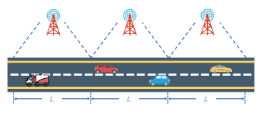
Figure 1: An illustration of the V2I networks with inter-site distance $L$.

III System Model And Problem Formulation

This section presents the overall system model in V2I networks with edge computing, and formulates a joint computation offloading and resource allocation optimization problem. For the sake of convenience, the main notations used are summarized in Table I.

III-A System Model

As shown in Fig. 1, we consider the V2I network in which an arbitrary vehicle drives on the highway and is connected to the RSU. The RSUs are evenly spaced along the highway and have the same coverage $L$, and the vehicle’s velocity denoted by $v$ is time-varying. Edge servers with abundant computation resources are deployed in these RSUs.

A computation-intensive application for one in-vehicle user equipment (UE) can be partitioned into $N$ tasks with the dynamic partitioning scheme [11]. As shown in Fig. 2, the inter-dependency between tasks is captured by a directed acyclic graph (DAG) $G=(V,E)$. Each node $i\in V$ represents a task and a directed edge $e(i,j)\in E$ indicates the precedence constraint between task $i$ and $j$, which means the execution of task $j$ cannot begin until its precedent task $i$ is completely processed.

Each task $i$ can be described by a three-tuple $\varphi_{i}=(DI_{i},DO_{i},C_{i})$, where $DI_{i}$ and $DO_{i}$ represent the input and output data size of task $i$ respectively, $C_{i}$ is the required CPU cycles to complete task $i$. We denote $k_{i}\in\{0,1\}$ as the offloading decision of task $i$, and specifically, $k_{i}=0$ means that the UE decides to execute task $i$ locally while $k_{i}=1$ implies that the UE chooses to offload task $i$ to the edge server. The wireless communication between the UE and RSUs is based on IEEE 802.11p VANET [24]. It should be noted that the UE can only access to RSU $m$ when the vehicle runs within its coverage.

III-B Local Computing

With the technique of dynamic voltage and frequency scaling (DVFS) [25], the UE can assign different computational capability for different tasks. We denote the CPU frequency for computing task $i$ as $f_{i}$ with $f_{i}\leq f_{max}^{l}$, where $f_{max}^{l}$ is the peak CPU frequency of the UE. Then the execution time of task $i$ for local computation is given by

$$t_{i}^{l}=\frac{C_{i}}{f_{i}},$$

and the energy consumption for task $i$ is given by

$$e_{i}^{l}=\kappa C_{i}f_{i}^{2},$$

where $\kappa$ is the effective switched capacity parameter depending on the chip architecture [3].

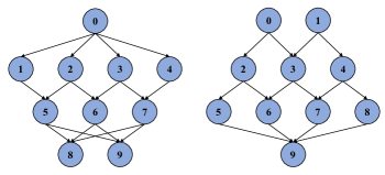
Figure 2: Directed acyclic graphs.

III-C Edge Computing

For the edge computing, the UE will offload task $i$ to the edge server, and then the edge server will execute the computation task and return the results to the UE. Therefore, the offloading process of task $i$ includes three phases in sequences: the offloading phase, the edge execution phase and the downloading computing outputs phase.

1) Offloading phase: According to Shannon’s Theorem, the uplink rate for offloading task $i$ is expressed as

$$R_{i}^{u}=W\log_{2}(1+\frac{p_{i}G_{A}h_{i}}{\sigma^{2}}),$$

where $W$ is the channel bandwidth, $p_{i}$ is the transmit power when offloading task $i$ to the RSU, $G_{A}$ is the antenna gain, $h_{i}$ is the channel gain including the large scale and small scale effect, and $\sigma^{2}$ is the power of white Gaussian noise. Our algorithm can be applied to any channel model. In the later experiments of this paper, exponential loss channel model is adopted.

Accordingly, the transmission delay and the energy consumption during the transmission phase of task $i$ can be expressed as

$$t_{i}^{u}=\frac{DI_{i}}{R_{i}^{u}},$$

and

$$e_{i}^{u}=p_{i}t_{i}^{u}.$$

2) Edge execution phase: We assume the edge server possesses abundant computation resources, and its CPU frequency $f^{e}$ is fixed and does not change during the execution process. In practical cases, it is assumed that the edge server has superior computation capability over the UE, and therefore $f^{e}>f_{max}^{l}$. Then the execution time of task $i$ in the edge server can be computed as

$$t_{i}^{e}=\frac{CI_{i}}{f^{e}}.$$

3) Downloading computing outputs phase: As for the downlink transmission, we denote the transmit power of RSU as $p_{d}$, which keeps the same across all RSUs. Likewise, the downlink rate for returning the computing outputs of task $i$ to the vehicle is given by

$$R_{i}^{d}=W\log_{2}(1+\frac{p_{d}G_{A}h_{i}}{\sigma^{2}}).$$

As a result, the downlink transmission time during the receiving phase can be computed as

$$t_{i}^{d}=\frac{DO_{i}}{R_{i}^{d}}.$$

In order to avoid the task migration between adjacent RSUs, the execution of a task should be completed before the vehicle shifts from the current connected RSU to an adjacent one. We can express this constraint as

$$d_{i}+\int_{T_{i}^{s}}^{T_{i}^{e}}v\,dv<R,$$

where $d_{i}$ denotes the distance between the UE and the starting point of the connected RSU when task $i$ is offloaded to the edge server, $T_{i}^{s}$ and $T_{i}^{e}$ are the start time and the end time of task $i$.

When the task migration occurs, it can lead to a large propagation delay between neighbouring RSUs, which can be calculated as

$$t_{i}^{p}=t_{p}\cdot\mathbb{I}(d_{i}+\int_{T_{i}^{s}}^{T_{i}^{e}}v\,dv>R),$$

where $t_{p}$ is the constant propagation delay and $\mathbb{I}(\cdot)$ is the indicator function.

In light of the above three phases, we can evaluate the aggregate execution time of task $i$ as

$$t_{i}^{o}=t_{i}^{u}+t_{i}^{e}+t_{i}^{d}+t_{i}^{p}.$$

Assuming that all RSUs have enough energy to execute offloaded tasks and do not take into account the energy consumed during edge execution phase and downlink transmission phase, the energy consumption of the vehicle in edge computing results only from the uplink transmission, which is given by

$$e_{i}^{o}=e_{i}^{u}.$$

When offloading a task to the edge server, the UE pays for using the computation resources, and a higher resource demand leads to a higher payment. Our method can be adjusted for different charging methods. In this paper, we consider a linear pricing scheme and the cost $c_{i1}^{o}$ of executing task $i$ in the edge server can be computed as

$$c_{i}^{o}=C_{i1}u_{r},$$

where $u_{r}$ is the unit price charged for unit computation resource by the edge server. On the contrary, the UE does not need to pay for the service when executing the task locally with its own computation resource. Besides, a relatively high cost will be charged for the task migration service, which can be computed by

$$c_{i}^{m}=C_{i2}u_{m}\cdot\mathbb{I}(d_{i}+\int_{T_{i}^{s}}^{T_{i}^{e}}v\,dv>R),$$

where $u_{m}$ is the per-unit price of task migration and $C_{i2}$ is the necessary resource consumed for migration. It is only depended on the task itself.

III-D Task Dependency Model

As shown in Fig. 2, the precedence constraints among tasks regulate the execution order of tasks. Based on the offloading decision of the UE, the relation between the start time $T_{i}^{s}$ and the end time $T_{i}^{e}$ of task $i$ can be derived as

$$T_{i}^{e}=T_{i}^{s}+(1-k_{i})t_{i}^{l}+k_{i}t_{i}^{o}.$$

Task $i$ can be executed when all its immediate predecessors have completed. This constraint can be written as

$$T_{i}^{s}\geq\max_{j\in pred(i)}T_{j}^{e},$$

where $pred(i)$ denotes the set of immediate predecessors of task $i$.

III-E Problem Formulation

The main objective of this paper is to minimize the time-energy-service cost (TESC), which is evaluated as the weighted sum of the execution time and the energy consumption of the entire application and the charge for edge computing service. According to the offloading decision of the UE, the execution time and the energy consumption of task $i$ are denoted as

$$t_{i}=(1-k_{i})t_{i}^{l}+k_{i}t_{i}^{o},$$

and

$$e_{i}=(1-k_{i})e_{i}^{l}+k_{i}e_{i}^{o},$$

respectively. The charge for edge computing service solely depends on the offloaded tasks, which is given by

$$c_{i}=k_{i}(c_{i}^{o}+c_{i}^{m}).$$

Therefore, the TESC of all the tasks can be computed as

$$U=\sum_{i=1}^{N}(\beta_{1}t_{i}+\beta_{2}e_{i}+\beta_{3}c_{i}),$$

where $0\leq\beta_{1},\beta_{2},\beta_{3}\leq 1$ denote the weighting parameters, and $\beta_{1}+\beta_{2}+\beta_{3}=1$ without loss of generality.

We aim to minimize the TESC of all the tasks by optimizing the task offloading policy $\mathcal{K}\triangleq\{k_{i}\}$, local CPU frequency control policy $\mathcal{F}\triangleq\{f_{i}\}$ and transmit power allocation policy $\mathcal{P}\triangleq\{p_{i}\}$. The optimization problem can be formulated as a constrained minimization problem:

$$\min_{\mathcal{Y},\mathcal{K},\mathcal{P},\mathcal{F}}\quad U$$

s.t. $$\mathrm{C}1:y_{i}\in\{1,...,N\},$$

$$\mathrm{C}2:k_{i}\in\{0,1\},$$

$$\mathrm{C}3:0\leq f_{i}\leq f_{max}^{l},$$

$$\mathrm{C}4:0\leq p_{i}\leq p_{max},$$

$$\mathrm{C}5:\max_{j\in pred(i)}T_{j}^{e}\leq T_{i}^{s},$$ (24)

where $p_{max}$ is the peak transmit power of the UE. Constraint C1 indicates the serial number of each task. We use $y_{i}$ to denote the $i$-th execution task. Constraint C2 guarantees that each task is executed locally or offloaded to the edge server. Constraints C3 and C4 specify the computation resource limit and transmit power limit respectively. Constraint C5 ensures that task $i$ cannot start execution until all its immediate predecessors have been executed. It can be seen that problem (24) is a mixed-integer programming involving the integer variable $\mathcal{Y}$ and $\mathcal{K}$ and continuous variable $\mathcal{P}$ and $\mathcal{F}$, which is non-convex and NP-hard.

IV Design

In this section, we design a novel scheme to solve the problem (III-E). A GNN with attention mechanism is introduced to extract high-level features from the DAG. To deal with the hierarchical action space, we put forward a novel DRL algorithm. The selection of both discrete and continuous actions can be made with a single parametrized network.

IV-A Graph Attention Network

Convolutional neural networks (CNNs) and recurrent neural networks (RNNs) have been successfully applied to tackle machine learning tasks, mainly attributed to their great power of extracting high-level features from Euclidean data (e.g. images, text and videos). However, the complex relationships and interdependency between objects in graph data, such as the DAG in Fig. 2, have imposed significant challenges on existing machine learning algorithms [26].

With the introduction of attention mechanism, graph attention networks (GAT) has shown its computation efficiency and superior performance in dealing with graph data [27]. Compared with spectral-based GNN such as graph convolution network (GCN) [28], GAT can operate on directed graph without depending on upfront access to the entire graph structure. Accordingly, we utilize GAT to explore the hidden features of each task and the inter-dependency among them.

Our proposed GAT consists of one layer with ReLU as the activation function. Considering that the number of sub-tasks of an in-vehicular application is usually no more than 20, one-layer GAT has enough power to extract the information of the DAG. The input of the GAT is the matrix composed of node feature and the adjacent matrix. $\mathbf{h}=\{\vec{h}_{1},\vec{h}_{2},\dots,\vec{h}_{N}\},\vec{h}_{i}\in\mathbb{R}^{F}$, where $F$ is the number of features in each node. Specially, the features of each node in the input layer are represented by $\vec{h}_{i}=\{DI_{i},DO_{i},C_{i},E_{i},CO,n,\vec{v}\}$, where the first three features corresponds to the three-tuple $\varphi_{i}$, $E_{i}$ indicates whether task $i$ has been executed, $CO$ indicates the coordinate of the car, $n$ indicates how many tasks have not been executed and vector $\vec{v}$ indicates the recorded speed of the last five seconds. The input features are transformed into high-level features through a shared linear transformation, which is parameterized by a weight matrix $\mathbf{W}\in\mathbb{R}^{F\times F^{\prime}}$, where $F^{\prime}$ denotes the number of new generated features. Besides, we perform a shared attention mechanism $a:\mathbb{R}^{F^{\prime}}\times\mathbb{R}^{F^{\prime}}\to\mathbb{R}$ to assign different importance for each node pair. The attention coefficients $e_{ij}$, which indicates the importance of node $j$’s features to node $i$, can be computed as

$$e_{ij}=a(\mathbf{W}\vec{h}_{i},\mathbf{W}\vec{h}_{j}).$$

The shared attention mechanism $a$ is represented by a single-layer fully-connected network. At the output layer, we calculate the normalized attention coefficients $e^{\prime}_{ij}$ by using the softmax function across the neighbors of $i$ (including $i$ itself):

$$e^{\prime}_{ij}=\frac{\exp(e_{ij})}{\sum_{k\in\mathcal{N}_{i}\cup i}\exp(e_{ik})},$$

where $\mathcal{N}_{i}$ denotes the set of neighbors of node $i$. For better feature extraction result, we employ the multi-head attention mechanism by independently executing attention mechanism $a(\cdot,\cdot)$ several times and then concatenating their results. The output node features $\vec{h}^{\prime}_{i}$ after the multi-head attention can be computed by

$$\vec{h}^{\prime}_{i}=\bigg{|}\bigg{|}_{k=1}^{K}ReLU(\sum_{j\in\mathcal{N}_{i}\cup i}({e^{\prime}_{ij}}^{k}\mathbf{W}^{k}\vec{h}_{j}),$$

where $||$ is the concatenation operation, $K$ is the number of attention heads, and ${e^{\prime}_{ij}}^{k}$ is the normalized attention coefficients of the $k$-th attention head and $\mathbf{W}^{k}$ is the corresponding weight matrix. With the operations stated above, the dimension of node features is scaled from $F$ to $KF^{\prime}$.

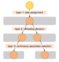
Figure 3: Hierarchical action space.

IV-B Hierarchical Action Space

As described in Section III-E, the action space of the UE exhibits a hierarchical structure. As shown in Fig. 3, the hierarchical action space can be divided into three parts:

• layer 1: task assignment. The UE needs to decide which task to be assigned without breaking the constraints of task dependency (Section III-D).

• layer 2: offloading decision. The UE needs to decide the assigned task to be executed locally or offloaded to the edge server.

• layer 3: continuous parameter selection. If the UE decides to execute the task locally, it should consider assigning how much CPU frequency to process the task. Likewise, if the UE offloads the task to the edge server, the appropriate transmit power should be allocated.

Most of existing DRL algorithms require the action space to be either discrete (e.g. DQN [18] and A3C [29]) or continuous (e.g. DPG [30] and DDPG [31]). There are two straightforward ideas to apply these traditional DRL algorithms on discrete-continuous hybrid action space. The first is to approximate the continuous part by a finite discrete set. However, this method narrows the continuous action space and the fine-grained approximation requires complicated design. The second is to relax the discrete part to a continuous set and apply DDPG algorithm subsequently. Compared with the original action space, this approach significantly increases its complexity. In our problem, task dependency makes a large number of invalid actions in every step of decision making. DDPG cannot mask invalid actions and can only impose a large penalty on invalid actions. Our experiments indicates that low sampling efficiency makes it hard for DPPG to converge. Also, study[41] points out that when invalid action space is too large, imposing great negative penalty on invalid actions will not work.

Inspired by normalized advantage functions (NAF) [32], we design a novel DRL algorithm, named parameterized NAF (PNAF), which directly works on hierarchical action space containing both discrete and continuous actions directly without approximation or relaxation.

For a simple illustration, the hierarchical action space in our paper is expressed as

$$A=\{a_{d},a_{c}\}=\{(y_{i},k_{i}=0,f_{i})\cup(y_{i},k_{i}=1,p_{i})\},$$

where $a_{d}$ represents the discrete action set and $a_{c}$ represents the continuous action set. We denote the action selected at time $t$ by $a_{t}=(y_{t},k_{t},f_{t},p_{t})$ and the corresponding action-value function by $Q(s_{t},a_{t})$, where $s_{t}\in\mathcal{S}$, $y_{t}\in\mathcal{Y}$, $k_{t}\in\mathcal{K}$, $f_{t}\in\mathcal{F}$ and $p_{t}\in\mathcal{P}$. The Bellman equation in the hierarchical action space $A$ is given by

$$Q(s_{t},a_{t})=\mathbb{E}[r_{t}+\gamma\max_{y_{t+1}}\max_{k_{t+1}}\sup_{f_{t+1},p_{t+1}}Q(s_{t+1},a_{t+1})],$$

where $r_{t}$ is the immediate reward and $\gamma$ is the discount factor. However, in hierarchical action space, the action-value function $Q(s,a)$ suffers from the problem of over-parameterization, which is written as

$$Q(s,a)=\begin{cases}Q(s,y,k,f),&\text{if $k=0$},\\ Q(s,y,k,p),&\text{if $k=1$}.\end{cases}$$

In other words, the action-value function $Q(s,a)$ is influenced by irrelevant continuous parameters.

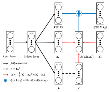
Figure 4: The architecture of the parameterized network.

To overcome the over-parameterization problem, we introduce a novel neural network shown in Fig. 4, which separately outputs a state value function term $V(s,a_{d})$ and an advantage term $A(s,a_{d},a_{c})$. The former term $V(s,a_{d})$ represents the expected cumulative reward when a discrete action $a_{d}$ is decided, and the latter term $A(s,a_{d},a_{c})$ represents the difference between the expected cumulative reward when a deterministic continuous $a_{c}$ is taken and $V(s,a_{d})$. Therefore, the final Q-function $Q(s,a_{d},a_{c})$ can be computed as

$$Q(s,a_{d},a_{c})=Q(s,a_{d})+A(s,a_{d},a_{c}).$$

Accordingly, the Bellman equation in Equation (29) becomes

$$Q(s_{t},a_{d_{t}},a_{c_{t}})=\mathbb{E}\{ r_{t}+\gamma\max_{a_{d_{t+1}}}\sup_{a_{c_{t+1}}}[V(s_{t+1},a_{d_{t+1}})+$$ (32)

$$A(s_{t+1},a_{d_{t+1}},a_{c_{t+1}})]\}.$$

Since the state value function $V(s_{t+1},a_{d_{t+1}}))$ is irrelevant with the continuous action $a_{c_{t+1}}$, it can be taken out of the operation of taking supremum over continuous action space, and therefore Equation (32) can be rewritten as

$$Q(s_{t},a_{d_{t}},a_{c_{t}})=\mathbb{E}\{ r_{t}+\gamma\max_{a_{d_{t+1}}}[V(s_{t+1},a_{d_{t+1}})+$$ (33)

$$\sup_{a_{c_{t+1}}}A(s_{t+1},a_{d_{t+1}},a_{c_{t+1}})]\}.$$

To guarantee the optimality of the continuous action that maximizes the advantage function, we restrict the advantage function $A(s,a_{d},a_{c})$ as a quadratic function of the estimated continuous action $a_{c}(s;\theta)$:

$$A(s,a_{d},a_{c};\theta)=-\frac{1}{2}(a_{c}^{\prime}-a_{c}(s;\theta))^{T}P(s;\theta)(a_{c}^{\prime}-a_{c}(s;\theta)).$$

The positive-definite square matrix $P(s;\theta)$ can be computed by Cholesky decomposition:

$$P(s;\theta)=L(s;\theta)L(s;\theta)^{T},$$

where $L(s;\theta)$ is a lower-triangular matrix with positive diagonal terms. The state-dependent entries of $L(s;\theta)$ come from the output layer of the neural network.

In order to encourage the agent to explore the discrete action space sufficiently and discover a better policy, the selection of discrete actions is based on $\epsilon$-greedy policy. The agent will choose a random action from its action space with probability $\epsilon$ or choose the action with the highest $V$-value with probability $1-\epsilon$. The assignment of $a_{d}$ is given by

$$a_{d}=\begin{cases}\text{a random action}&\text{with probability $\epsilon$}\\ \arg\max_{a_{d}}V(s,a_{d};\theta)&\text{with probability $1-\epsilon$}\end{cases}$$

As for the continuous action, the Ornstein-Uhlenbech (OU) process is introduced to generate a temporally correlated noise sequence. The appendix specifies how the reinforcement learning with discrete-continuous hybrid action space operates.

IV-C Deep Reinforcement Learning

By combining the deep learning (DL) [33] and RL [13], DRL aims at constructing an agent that can acquire knowledge by exploring the interaction with the environment without the need of external supervision in an end-to-end manner [14]. DRL can be modeled as Markov Decision Process (MDP) which is represented by a four-tuple $M=\{S,A,P,R\}$, where $S$ is the state space, $A$ is the action space, $P$ is the transition probability matrix and $R$ is the reward function. At each time step $t$, the agent observes the current environment state $s_{t}$ and chooses an action $a_{t}$ following a stochastic policy $\pi:S\to A$, which maps state space $S$ to a probability distribution over action space $A$. Then the environment state changes to $s_{t+1}$ with probability $p(s_{t+1}|s_{t},a_{t})$, and the agent receives an immediate reward $r_{t}(s_{t},a_{t},s_{t+1})$, which indicates the effect of action $a_{t}$ on state $s_{t}$. The goal of the agent is to maximize the cumulative discounted reward $R_{t}=\sum_{t=0}^{T}\gamma^{t}r_{t}$, where $\gamma$ is the discounted factor and $T$ is the end episode. We define the state-value function under policy $\pi$ as $V^{\pi}(s)=\mathbb{E}[\sum_{t=0}^{T}\gamma^{t}r_{t}|\pi]$, which denotes the expected total discounted reward at state $s$. Through episodic interactions with the environment, the agent tries to find the optimal policy $\pi^{*}$ that achieves the optimal action value function $V^{*}$.

The vehicular offloading problem can be modelled as an MDP and the definition of each element in reinforcement learning are introduced as follows:

State space. The state space is composed of two parts: the task state and the environment state. We present both parts of the information in the DAG. So the node feature of the DAG is $\mathbf{h}_{t}=\{\vec{h}_{1},\vec{h}_{2},\dots,\vec{h}_{N}\}$ with $\vec{h}_{i}=\{DI_{i},DO_{i},C_{i},E_{i},CO,n,\vec{v}\}$.

Action space. As described in Section IV-B, the action space has a hierarchical structure and is composed of task assignment $y_{t}$, offloading decision $k_{t}$, local CPU frequency $f_{t}$ and transmit power $p_{t}$.

Reward. Our objective is to minimize the TESC of the whole application, we set the reward of each action as the negetive immediate TESC achieved by the executed task $y_{t}$.

$$r_{t}=-(\beta_{1}t_{y_{t}}+\beta_{2}e_{y_{t}}+\beta_{3}c_{y_{t}}).$$

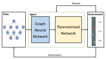
Figure 5: The architecture of the proposed DHVO solution.

Algorithm 1 Deep Hierarchical Vehicular Offloading (DHVO)

  Input: DAG of tasks and node feature vector $\mathbf{h}_{t}=\{\vec{h}_{1},\vec{h}_{2},\dots,\vec{h}_{N}\}$ with $\vec{h}_{i}=\{DI_{i},DO_{i},C_{i},E_{i},CO,n,\vec{v}\}$.

  Output: task assignment $y_{t}$, offloading decision $k_{t}$, local CPU frequency $f_{t}$ and transmit power $p_{t}$

  

  // initialization

  Randomly initialize the parameters in graph neural network and parameterized network $Q(s,a;\theta_{g},\theta_{p})$

  Initialize target network $Q^{\prime}(s,a;\theta_{g}^{\prime},\theta_{p}^{\prime})$ with weight $\theta_{g}^{\prime}\leftarrow\theta_{g}$ $\theta_{p}^{\prime}\leftarrow\theta_{p}$

  Initialize replay buffer $D\leftarrow\varnothing$

  

  // training process

  for episode = 1, $M$ do

     for t = 1, $T$ do

        Observe current state $s_{t}$

        Select hierarchical action $a_{t}$

        Execute $(y_{t},k_{t}=0,f_{t})$ or $(y_{t},k_{t}=1,p_{t})$

        Observe next state $s_{t+1}$ and receive reward $r_{t}$

        Store transition $(s_{t},a_{t},r_{t},s_{t+1})$ in $D$

        Sample a random batch $(s_{i},a_{i},r_{i},s_{i+1})$ from $D$

        Set target value $z_{i}=r_{i}+\gamma\max_{a_{d}}V^{\prime}(s_{i+1},a_{d};\theta_{p})$

        Set loss function $L_{t}=(z_{i}-Q(s_{i},a_{i};\theta_{g},\theta_{p}))^{2}$

        Update network parameters: $\theta_{g}\leftarrow\theta_{g}+\alpha_{g}\nabla_{\theta_{g}}L_{t}$, $\theta_{p}\leftarrow\theta_{p}+\alpha_{p}\nabla_{\theta_{p}}L_{t}$ and $\theta_{g}^{\prime}\leftarrow\theta_{g}$, $\theta_{p}^{\prime}\leftarrow\tau\theta_{p}+(1-\tau)\theta_{p}^{\prime}$

     end for

  end for

IV-D Deep Hierarchical Vehicular Offloading

By introducing the technique of GAT and PNAF into DRL, we propose an adaptive vehicular offloading algorithm named Deep Hierarchical Vehicular Offloading (DHVO). The framework of DHVO is illustrated in Fig. 5. The decision-making of a UE consists of a graph neural network and a parameterized network, which establishes the mapping between a state and a hierarchical action.

The pseudo-code of DHVO is shown in Algorithm 1. We first initialize the graph neural network and parameterized network $Q(s,a;\theta_{g},\theta_{p})$ and its target network $Q^{\prime}(s,a;\theta_{g}^{\prime},\theta_{p}^{\prime})$ with $\theta_{g}^{\prime}=\theta_{g}$ and $\theta_{p}^{\prime}=\theta_{p}$. The replay buffer $D$ is set to $\varnothing$ initially.

At each decision epoch $t$ when the UE finishes the last task $TASK_{t-1}$ and starts the execution of a new task $TASK_{t}$, the UE will observe the new state $\mathbf{h}_{t}=\{\vec{h}_{1},\vec{h}_{2},\dots,\vec{h}_{N}\}$ with $\vec{h}_{i}=\{DI_{i},DO_{i},C_{i},E_{i},CO,n,\vec{v}\}$. The GAT will extract the high-level features and encode the state to a vector. With the procession of the GAT, the vector can present the state information better. And the policy network will outputs the hierarchical action $a_{t}\in\{(y_{t},k_{t}=0,f_{t})\cup(y_{t},k_{t}=1,p_{t})\}$ and corresponding Q-value $Q(s_{t},a_{t};\theta_{g},\theta_{p})$. After carrying out the selected action, the state turns into $s_{t+1}$ and the UE receives the immediate reward $r_{t}$. The UE will record the environment transition $(s_{t},a_{t},s_{t+1},r_{t})$ into the replay buffer D.

Table II: Simulation Parameters

Description	Parameter	Value
Coverage of each RSU	$L$	200 m
Length of time-slot	$\Delta t$	1 s
Number of tasks	$N$	8-12
Input datasize of each task	$DI$	[2.5, 3.5] MByte
Output datasize of each task	$DO$	[2.5, 3.5] MByte
Required computation resources	$C$	[800, 1200] Mcycles
Bandwidth	$W$	2 MHz
Peak local computing capability	$f^{l}_{max}$	$10^{8}$ cycles/s
Edge server computing capability	$f^{e}$	$10^{9}$ cycles/s
Peak transmit power	$p^{l}_{max}$	200 mW
Computing efficiency parameter	$\kappa$	$10^{-25}$
Atenna gain	$G_{A}$	4.11
Distance from the RSU	$d$	100 m
Constant propagation delay	$t_{p}$	5 s
Carrier frequency	$F_{c}$	915 MHz
Path loss exponent	$PL$	3
Noise power	$\delta^{2}$	$10^{-12}$ W
Computation resource price	$u_{r}$	0.1 $/Mcycles
Task migration price	$u_{m}$	2 $/Mcycles
System cost weighting parameters	$\beta_{1},\beta_{2},\beta_{3}$	0.33, 0.33, 0.33

At the beginning of parameter update, a training batch $(s_{i},a_{i},s_{i+1},r_{i})$ is sampled randomly from $D$. As for the graph neural network $Q(\theta_{g},\theta_{p})$, the target value $z_{i}$ is set to the sum of the immediate reward $r_{i}$ and the highest $V$-value of target network $Q^{\prime}(\theta_{g}^{\prime},\theta_{p}^{\prime})$:

$$z_{i}=r_{i}+\gamma\max\limits_{a_{d}}V^{\prime}(s_{i+1},a_{d};\theta_{p}^{\prime}),$$

where $\gamma$ is the discount factor. In order to adjust the estimated $Q$-value toward the target value, we update the parameters of $Q$ by minimizing the mean squared error between the target value $z_{i}$ and its current output. The loss function $L_{t}$ is given by

$$L_{t}=(z_{i}-Q(s_{i},a_{i};\theta_{g},\theta_{p}))^{2},$$

Then we perform gradient descent to update the parameters of three neural networks as below:

$$\theta_{g}\leftarrow\theta_{g}+\alpha_{g}\nabla_{\theta_{g}}L_{t},$$

$$\theta_{p}\leftarrow\theta_{p}+\alpha_{p}\nabla_{\theta_{p}}L_{t},$$

$$\theta_{g}^{\prime}\leftarrow\theta_{g}$$

$$\theta_{p}^{\prime}\leftarrow\tau\theta_{p}+(1-\tau)\theta_{p}^{\prime},$$

where $\alpha_{g}$ and $\alpha_{p}$ are the learning rates of the graph neural network $\theta_{g}$ and the parameterized network $\theta_{p}$, and $\tau$ is the soft-update coefficient of the target network. In this way, the network parameters are updated with episodic training until convergence.

Table III: Parameters of neural networks

Parameter	Value
Attention heads of GAT	2
Number of features of each attention head	6
Network hidden layers of parameterized network	128
Reward discounted factor	0.99
Learning rate of parameterized network	0.01
Soft-update coefficient of the target network	0.1
Activation function	ReLU
Network optimizer	Adam
Max training episodes	20
Batch size	256

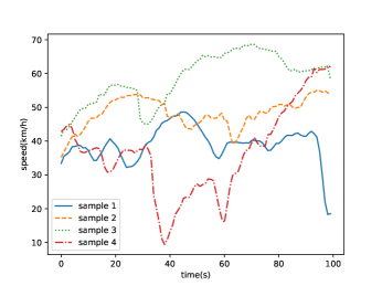
Figure 6: Four samples of speed trajectories.

V Evaluation

V-A Simulation Setup

Simulation environment. We consider one vehicle running on the highway along which several APs are evenly deployed with coverage $R=200$ m. The speed of the vehicle is collected from a real-world dataset provided by CPIPC (China Postgraduate Innovation & Practice Competition) [34]. The speed data collection lasts for seven days and is measured in seconds. We tailor this dataset to four trajectories, each of which contains 100s speed data. As shown in Fig. 6, the speed of the vehicle varies with time dynamically and therefore is hard to predict. In the experiment, we did not set a specific type of task, although setting a type of task could better describe the workload. The input data size $DI_{i}$, output data size $DO_{i}$ and required computation resources $C_{i}$ follows uniform distribution in the range of [2.5, 3.5] MBytes, [2.5, 3.5] MBytes and [800, 1200] Mcycles, respectively. The line-of-sight channel gain $h_{i}$ follows $h_{i}=(\frac{3\times 10^{8}}{4\pi F_{c}d_{i}})^{PL}$, in which $F_{c}$ denotes the carrier frequency, $d_{i}$ denotes the distance between the UE and the RSU, and $PL$ denotes the path loss exponent. The complete simulation parameters are shown in Table II and are set as default unless otherwise specified.

Neural network parameters. The neural network consists of two parts. The first part is a one-layer GAT consisted of $K=2$ attention heads computing $F^{\prime}=6$ features (for a total of 12 features). The GAT part encodes a state vector with high level feature of application graph. Since the length of the vector will vary with the node number of the graph. We use the padding method to obtain the state vector with a fixed length. The second part is parameterized network which is fully connected with one hidden layer containing 128 neurons. We set the learning rate 0.01 separately, and set the soft-update coefficient of the target network to 0.1. The reward discounted factor $\gamma$ is set to 0.99. We use Rectified Linear Unit (ReLU) as the activation function and Adam as the optimization algorithm. The detailed parameters setting of the neural network is listed in Table III.

Simulation platform. We implemented DHVO algorithm based on Pytorch library with Python 3.5. The simulation platform is a Ubuntu Server 16.04 with 32GB RAM and an Intel (R) Core (TM) i7-6800K CPU, which has 6 cores and 12 threads.

Compared algorithms. We compare our proposed algorithm DHVO with three representative benchmarks:

• All locally executed (ALE): All of the tasks are executed locally with peak local computing capability;

• All offloaded (AO): All of the tasks are offloaded to the edge server with peak transmit power;

• Greedy on edge (GOE): The UE will offload the task to the edge server with peak transmit power if it predicts that the task can be returned within the coverage of the current RSU based on a constant speed (30 km/h). Otherwise, the UE will execute the task locally with peak local computing capability.

• Ddiscretization and DQN(DQN10): We approximate the continuous part by a finite discrete set, specifically the continuous interval represented by 10 equally spaced values. We use a GAT to encode the state and send it to the DQN neural network for training.

V-B Convergence Speed

In our experiments, we set each episode to execute twenty applications, and each application randomly consists of 8 to 12 sub-tasks. Set the neural network to starting training when there are more than 500 environment transitions in the buffer. We set the batch size to 256. Experiments show that our neural network converge within 14 episodes which can be seen in Fig. 7. And it takes only 1.58s to train a batch and 0.0018s to perform and inference.

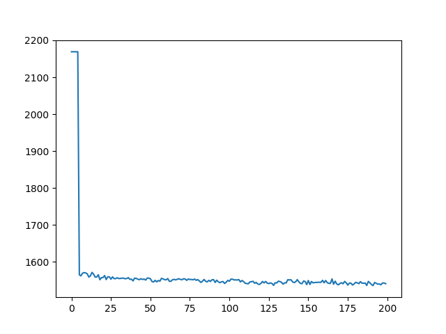
Figure 7: Convergence Curve

V-C Performance Evaluation

In this part, we evaluate the performance of five algorithms under different environment parameters and explore the relationship between the system cost and these parameters. The environment parameters are set default as listed in Table II unless otherwise specified. For a fair comparison, the DQN10 and our DHVO network are only trained 40 episodes. In the experiment, we find that the performance of DQN10 is very unstable, while the DHVO algorithm performs stably. This means that under 40 episodes of training, DQN10 even can not converge well. Based on this our analysis focuses on the performance of three other baseline algorithms and our DHVO algorithm. We conduct 50 individual test and take the average value as the final result.

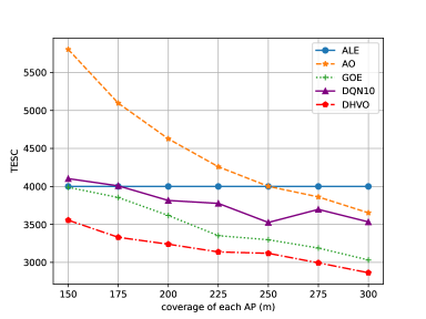
Figure 8: Total cost with the coverage of each RSU.

We varies the coverage of each RSU to find its relationship with the TESC of each algorithm. As shown in Fig 8, the system cost of each algorithm except for ALE decreases with the rising of RSU’s coverage. Since ALE executes all the tasks locally and does not involve the task offloading process, its system cost remains constant regardless of the change of RSU’s coverage. As for the other three algorithms, when the coverage of each RSU increases, the frequency of the task migration will decrease, which causes the cost reduction of task migration service. Compared with AO and GOE, the slope of DHVO is much smaller and therefore is less sensitive to the change of RSU’s coverage.

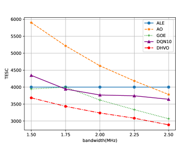
Figure 9: Total cost with bandwidth.

Fig. 9 indicates the system cost versus the bandwidth. Comparing ALE and AO, we can see that when the bandwidth is less than 2.25 MHz, the performance of ALE is much better than AO. Since the uplink/downlink rate and the bandwidth are in direct proportion relationship (Equation (5)(10)), the transmission time during the transmitting and receiving phase with low bandwidth is much longer than the local execution time. In addition, too long time spent in edge computing will increase the risk of the task migration. However, when the bandwidth keeps rising, edge computing shows its advantage of lower task completion time and therefore is more recommended than local execution. It can be clearly seen that DHVO is more robust to the change of the bandwidth than AO and GOE, which is attributed to its ability to forecast the occurrence of task migration.

Fig. 10(a) and Fig. 10(b) illustrate the relationship of the required computation resource and the input/output datasize with the system cost. We can find that the required computation resource of each task has more impact on local computing than edge computing, while the input/output datasize only affects edge computing. This is because the execution time and energy consumption during local execution are in direct proportion to the required computation resource (Equation (3)(4)), while the delay and energy during edge computing depends more on the data size of each task. Although edge servers can provide powerful computing capability, the risk of task migration will cause extra service cost and propagation delay. When the datasize is less than 2.5 MB, short transmission time during the transmitting and receiving phase can be achieved. Moreover, compared with GOE which prefers edge computing, DHVO can adjust its offloading policy based on tasks’ features and select proper offloading decision for each task.

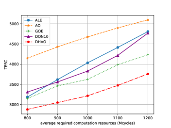
(a) Total cost with required computation resources.

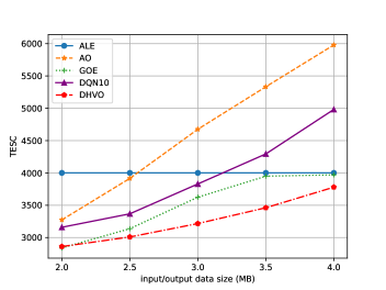
(b) Total cost with input / output data size.

Figure 10: Total costs for different required computation resources and input / output data sizes.

Fig. 11(a) and Fig. 11(b) illustrate the relationship between the system cost and the computation resource price and the task migration price respectively. Since all the tasks of ALE are executed locally and thus ALE needs not to pay for the edge computing service, the total cost of ALE remains constant in both cases. Comparing these two pictures, we can see that the task migration price has more impact on the performance of AO and GOE than the computation resource prices. The main reason is that the value of the former price is much higher than the latter price, and the occurrence of task migration will lead to extra payment. Although edge computing can achieve lower execution time and energy consumption, the high cost brought by frequent task migration in AO and GOE makes edge computing a poor choice. On account of much lower risk of task migration, DHVO is not affected by the change of the task migration price and performs quite better than AO and GOE.

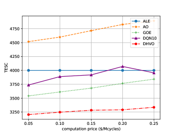
(a) Total cost with computation resource price.

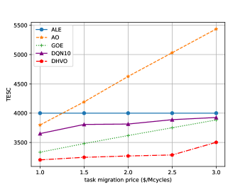
(b) Total cost with task migration price.

Figure 11: Total costs for different computation resource prices and task migration prices.

V-D Performance Analysis

In this part, we make a detailed analysis on the reasons why the performance of DHVO is much better than the compared algorithms from the perspective of the offloading policy and the TESC distribution of each algorithm.

Fig. 12 shows the number of each action taken by each algorithm when dealing with 200 application, each of which contains 8-12 tasks. We can find that DHVO makes a balance between local execution and edge computing, while GOE is greedy on offloading tasks to the edge server. However, since the speed of the vehicle varies dynamically, the constant speed used by GOE is wildly inaccurate compared with the real speed value, and accordingly GOE suffers a high penalty caused by task migration between consecutive RSUs. On the contrary, DHVO utilizes the speed data of last five seconds to make an accurate estimation on future speed, and thus avoids the occurrence of task migration. More precisely, if DHVO finds that the current task cannot be returned within the coverage of the current RSU when the vehicle runs at the predicted speed, it will decide to execute the task locally, and otherwise it will offload the task to the edge server to meet the low execution delay brought by edge computing.

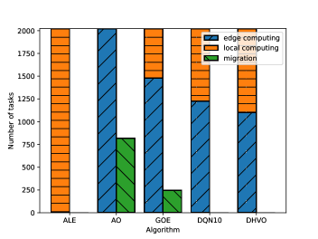
Figure 12: Action of each algorithm.

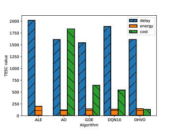
Figure 13: The cost value of each algorithm.

Fig. 13 depicts the cost distribution of each algorithm. We can see that the energy consumption of ALE is the highest among five algorithms, which explains the reasons why task offloading is necessary for energy conservation. As for AO, though edge computing brings lower task completion delay and energy consumption, it suffers from high cost of edge computation resource and task migration. In spite of lower probability of the task migration, GOE also suffers from high cost of task migration as a result of wrong speed estimation. As for DHVO, it learns to select proper offloading decision for each task by considering both the individual features of each task and the dynamic environment, and learns to select proper local computing capability and transmit power to make a balance among delay, energy and service cost.

Also we consider the effect of small fading, which obeys complex gaussian distribution. Specifically, the channel gain follows $h_{i}=\lambda(\frac{3\times 10^{8}}{4\pi F_{c}d_{i}})^{PL}$, where $\lambda$ indicates small scale fading. We show the experiment results in Fig.14 where the x-axis indicates the training episodes and y-axis indicates the TESC. Even though it this convergence curve is not as smooth as without small fading, our approach still enables learning.

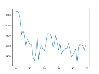
Figure 14: Convergence curve with small fading.

V-E Ablation Study

We conduct ablation study to figure out whether the graph attention network and PNAF training algorithm both contribute to the performance improvement. We use PNAF algorithm to train the neural network and do not use GAT to extract the graph information. We simply call this algorithm PNAF. We use GAT to extract the graph information and DQN to train. We call this algorithm GDQNX, where the ‘X’ indicates the size of the finite which approximates the interval [0, 1]. We compare the performance of several algorithms and normalize their performance. In fig. 15, DHVO outperforms both PNAF and any GDQNX algorithms which reflects that both GAT and PNAF are necessary for performance improvement. It is worth noticing that setting the finite set larger leading to worse performance, which is against common sense. The main reason is that each algorithm in the experiments trains the same number of episodes. Larger size means the network is more complex which requires more episodes of training to achieve optimal performance. So GDQN5 and GDQN10 do not converge well and perform worse.

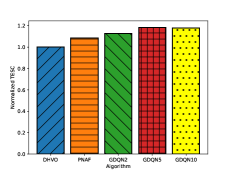
Figure 15: Ablation Study.

VI Conclusion

In this paper, we designed the joint computation offloading and resource allocation in V2I networks. The considered problem is formulated as a MINLP optimization by jointly optimizing the task assignment, task offloading decision, local computation resource allocation and power control. The system overhead was quantified by the time-energy-service cost (TESC), which is the weighted sum of execution time, energy consumption and charge of service. Based on DRL, we proposed a deep hierarchical vehicular offloading (DHVO) scheme to solve this problem in an end-to-end manner. With the help of graph neural networks, the hidden features of each sub-task and the interdependency between them were extracted. Moreover, we developed a novel neural network architecture to deal with the hierarchical action space which contains both discrete and continuous actions. The simulations have been conducted based on a real-world car speed dataset, and numerical results have shown that our proposed algorithm can significantly reduce the system cost under various environment parameters.

Xinyu You received the B.Eng. degree from the School of Electronic Information, Wuhan University, Wuhan, China, in 2018. He is currently pursuing the M.S. degree at Fudan University, Shanghai, China. His research interests include deep reinforcement learning, routing, and edge computing.

Haojie Yan received the B.Eng. degree from the School of Information Science and Technology, Fudan University, Shanghai, China, in 2021. He is currently pursuing the M.S. degree at Fudan University, Shanghai, China. His research interests include deep reinforcement learning, integer programming, and edge computing.

Yuedong Xu is a Professor with the School of Information Science and Technology, Fudan University, Shanghai, China. He received B.S. degree from Anhui University in 2001, M.S. degree from Huazhong University of Science and Technology in 2004, and Ph.D. degree from The Chinese University of Hong Kong, Hong Kong, China, in 2009. From late 2009 to 2012, he was a Postdoc with INRIA Sophia Antipolis and Universite d’Avignon, France. He has published more than 30 papers in reputable vents including ACM Mobisys, ACM Mobihoc, ACM CoNEXT, IEEE Infocom, IEEE/ACM ToN, IEEE TMC, etc. He served as TPC members in Mobihoc, PAM, IJCAI and WiOpt. His research interests include performance evaluation, machine learning, data analytics of communication networks, and mobile computing.

Lifeng Wang (M’16) is a faculty member at the Department of Electrical Engineering, Fudan University. He received the Ph.D. degree in Electrical Engineering from the Queen Mary University of London, U.K. He was a Research Associate with the Department of Electronic and Electrical Engineering, University College London (UCL), U.K. His research interests include ITS, 5G/6G systems, and information security. He received the Exemplary Editor Certificates of the IEEE Communications Letters in 2016, 2017 and 2018. Currently he serves as an associate editor in the IEEE Transactions on Intelligent Transportation Systems.

Liangui Dai Liangui Dai received Ph.D. degree in Control Theory and Application from Northeastern University, ShenYang, China in 1997. He is a senior researcher with the intelligent transportation system (ITS) research institute of Guangdong Litong Corp. His research interests include data analytics of ITS and information system development for ITS.

References

- [1] J. Zhang and K. B. Letaief, “Mobile edge intelligence and computing for the internet of vehicles,” IEEE Proc., vol. 108, no. 2, pp. 246-261, Feb. 2020.
- [2] Y. Wu et al., “Secrecy-driven resource management for vehicular computation offloading networks,” IEEE Netw., vol. 32, no. 3, pp. 84-91, May 2018.
- [3] P. Keshavamurthy, E. Pateromichelakis, D. Dahlhaus, and C. Zhou, “Edge cloud-enabled radio resource management for co-operative automated driving,” IEEE J. Sel. Areas Commun., vol. 38, no. 7, pp. 1515-1530, July 2020.
- [4] J. Yan, S. Bi, Y.-J. A. Zhang, and M. Tao, “Optimal task offloading and resource allocation in mobile-edge computing with inter-user task dependency,” IEEE Trans. Wireless Commun., vol. 19, no. 1, pp. 235-250, Jan. 2020.
- [5] Y. Mao, C. You, J. Zhang, K. Huang, and K. B. Letaief, “A survey on mobile edge computing: The communication perspective,” IEEE Commun. Surveys Tuts., vol. 19, no. 4, pp. 2322–2358, 2017.
- [6] X. Lyu et al., “Optimal schedule of mobile edge computing for Internet of Things using partial information,” IEEE J. Sel. Areas Commun., vol. 35, no. 11, pp. 2606–2615, Nov. 2017.
- [7] X. Hu, L. Wang, K. K. Wong, M. Tao, Y. Zhang, and Z. Zheng, “Edge and central cloud computing: A perfect pairing for high energy efficiency and low-latency,” IEEE Trans. Wireless Commun., vol. 19, no. 2, pp. 1070–1083, Feb. 2020.
- [8] S. Olariu, “A survey of vehicular cloud research: Trends, applications and challenges,” IEEE Trans. Intell. Transp. Syst., vol. 21, no. 6, pp. 2648–2663, June 2020.
- [9] J. Zhao, X. Sun, Q. Li and X. Ma, “Edge caching and computation management for real-time internet of vehicles: An online and distributed Approach,” IEEE Trans. Intell. Transp. Syst., vol. 22, no. 4, pp. 2183–2197, April 2021.
- [10] X. Huang, R. Yu, S. Xie, and Y. Zhang, ”Task-container matching game for computation offloading in vehicular edge computing and networks,” IEEE Trans. Intell. Transp. Syst., vol. 22, no. 10, pp. 6242–6255, Oct. 2021.
- [11] L. Yang, J. Cao, H. Cheng, and Y. Ji, “Multi-user computation partitioning for latency sensitive mobile cloud applications,” IEEE Trans. Comput., vol. 64, no. 8, pp. 2253–2266, Aug. 2015.
- [12] T. Q. Dinh, J. Tang, Q. D. La, and T. Q. Quek, “Offloading in mobile edge computing: Task allocation and computational frequency scaling,” IEEE Trans. Commun., vol. 65, no. 8, pp. 3571–3584, Aug. 2017.
- [13] R. S. Sutton and A. G. Barto, “Reinforcement learning: An introduction,” MIT press, 2018.
- [14] V. Mnih et al., “Playing atari with deep reinforcement learning,” NIPS Deep Learning Workshop, 2013, pp. 1-9.
- [15] S. Boyd, N. Parikh, and E. Chu, “Distributed optimization and statistical learning via the alternating direction method of multipliers,” Now Publishers Inc, 2011.
- [16] K. Zhang, Y. Mao, S. Leng, S. Maharjan, and Y. Zhang, “Optimal delay constrained offloading for vehicular edge computing networks,” IEEE Int. Conf. Commun. (ICC), 2017, pp. 1–6.
- [17] Z. Ning et al., “Joint computing and caching in 5G-envisioned internet of vehicles: A deep reinforcement learning-based traffic control system,” IEEE Trans. Intell. Transp. Syst., vol. 22, no. 8, pp. 5201–5212, Aug. 2021.
- [18] V. Mnih et al., “Human-level control through deep reinforcement learning,” Nature, vol. 518, no. 7540, pp. 529–533, Feb. 2015.
- [19] R. F. Atallah, C. M. Assi, and M. J. Khabbaz, “Scheduling the operation of a connected vehicular network using deep reinforcement learning,” IEEE Trans. Intell. Transp. Syst., vol. 20, no. 5, pp. 1669–1682, May 2019.
- [20] K. Zhang, Y. Zhu, S. Leng, Y. He, S. Maharjan, and Y. Zhang, “Deep learning empowered task offloading for mobile edge computing in urban informatics,” IEEE Internet Things J., vol. 6, no. 5, pp. 7635–7647, Oct. 2019.
- [21] Y. He, N. Zhao, and H. Yin, “Integrated networking, caching, and computing for connected vehicles: A deep reinforcement learning approach,” IEEE Trans. Veh. Technol., vol. 67, no. 1, pp. 44–55, Jan. 2018.
- [22] H. Van Hasselt, A. Guez, and D. Silver, “Deep reinforcement learning with double q-learning,” AAAI Conf., 2016, pp. 2094–2100.
- [23] Z. Wang, T. Schaul, M. Hessel, H. Hasselt, M. Lanctot, and N. Freitas, “Dueling network architectures for deep reinforcement learning,” Int. Conf. Mach. Learn. (ICML), 2016, pp. 1995–2003.
- [24] L. Yao, J. Wang, X. Wang, A. Chen, and Yuqi Wang, “V2X routing in a VANET based on the hidden markov model,” IEEE Trans. Intell. Transp. Syst., vol. 19, no. 3, pp. 889–899, Mar. 2018.
- [25] X. Lin, Y. Wang, Q. Xie, and M. Pedram, “Task scheduling with dynamic voltage and frequency scaling for energy minimization in the mobile cloud computing environment,” IEEE Trans. Serv. Comput., vol. 8, no. 2, pp. 175-186, 2015.
- [26] Z. Wu, S. Pan, F. Chen, G. Long, C. Zhang, and S. Y. Philip, “A comprehensive survey on graph neural networks,” IEEE Trans. Neural Netw. Learn. Syst., vol. 32, no. 1, pp. 4-24, Mar. 2020.
- [27] P. Veličković, G. Cucurull, A. Casanova, A. Romero, P. Liò, and Y. Bengio, “Graph attention networks,” Int. Conf. Learn. Represent. (ICLR), 2018, pp. 1–12.
- [28] T. N. Kipf and M. Welling, “Semi-supervised classification with graph convolutional networks,” Int. Conf. Learn. Represent. (ICLR), 2017, pp. 1–14.
- [29] V. Mnih et al., “Asynchronous methods for deep reinforcement learning,” Int. Conf. Mach. Learn. (ICML), 2016, pp. 1928–1937.
- [30] D. Silver, G. Lever, N. Heess, T. Degris, D. Wierstra, and M. Riedmiller, “Deterministic policy gradient algorithms,” Int. Conf. Mach. Learn. (ICML), 2014.
- [31] T. P. Lillicrap et al., “Continuous control with deep reinforcement learning,” Int. Conf. Mach. Learn. (ICML), 2016.
- [32] S. Gu, T. Lillicrap, I. Sutskever, and S. Levine, “Continuous deep q-learning with model-based acceleration,” Int. Conf. Mach. Learn. (ICML), 2016, pp. 2829–2838.
- [33] Y. LeCun, Y. Bengio, and G. Hinton, “Deep learning,” Nature, vol. 521, no. 7553, pp. 436–444, 2015.
- [34] China Postgraduate Innovation & Practice Competition (CPIPC) https://cpipc.chinadegrees.cn/
- [35] Z. Ali, L. Jiao, T. Baker, G. Abbas, Z. H. Abbas, and S. Khaf, “A deep learning approach for energy efficient computational offloading in mobile edge computing,” IEEE Access, vol. 7, pp. 149 623–149 633, 2019.
- [36] Z. Hong, W. Chen, H. Huang, S. Guo, and Z. Zheng, “Multi-hop cooperative computation offloading for industrial iot–edge–cloud computing environments,” IEEE Transactions on Parallel and Distributed Systems, vol. 30, no. 12, pp. 2759–2774, 2019.
- [37] C. Wang, C. Dong, J. Qin, X. Yang, and W. Wen, “Energy-efficient offloading policy for resource allocation in distributed mobile edge computing,” in 2018 IEEE Symposium on Computers and Communications (ISCC). IEEE, 2018, pp. 00 366–00 372.
- [38] H. Guo and J. Liu, “Collaborative computation offloading for multiaccess edge computing over fiber–wireless networks,” IEEE Transactions on Vehicular Technology, vol. 67, no. 5, pp. 4514–4526, 2018.
- [39] Y. Chen, F. Zhao, X. Chen, and Y. Wu, “Efficient multi-vehicle task offloading for mobile edge computing in 6g networks,” IEEE Transactions on Vehicular Technology, 2021.
- [40] T. Zhang and W. Chen, “Computation offloading in heterogeneous mobile edge computing with energy harvesting,” IEEE Transactions on Green Communications and Networking, vol. 5, no. 1, pp. 552–565, 2021.
- [41] S. Huang and S. Ontañón, “A closer look at invalid action masking in policy gradient algorithms,” arXiv preprint arXiv:2006.14171, 2020.
- [42] M. Hausknecht and P. Stone, “Deep reinforcement learning in parameterized action space,” arXiv preprint arXiv:1511.04143, 2015.
- [43] J. Xiong, Q. Wang, Z. Yang, P. Sun, L. Han, Y. Zheng, H. Fu, T. Zhang, J. Liu, and H. Liu, “Parametrized deep q-networks learning: Reinforcement learning with discrete-continuous hybrid action space,” arXiv preprint arXiv:1810.06394, 2018.
- [44] C. J. Bester, S. D. James, and G. D. Konidaris, “Multi-pass q-networks for deep reinforcement learning with parameterised action spaces,” arXiv preprint arXiv:1905.04388, 2019.