Chiral symmetry and Atiyah-Patodi-Singer index theorem for staggered fermions

Abstract

We consider the Atiyah-Patodi-Singer (aps) index theorem corresponding to the chiral symmetry of a continuum formulation of staggered fermions called Kähler-Dirac fermions, which have been recently investigated as an ingredient in lattice constructions of chiral gauge theories. We point out that there are two notions of chiral symmetry for Kähler-Dirac fermions, both having a mixed perturbative anomaly with gravity leading to index theorems on closed manifolds. By formulating these theories on a manifold with boundary, we find the aps index theorems corresponding to each of these symmetries, necessary for a complete picture of anomaly inflow, using a recently discovered physics-motivated proof. We comment on a fundamental difference between the nature of these two symmetries by showing that a sensible local, symmetric boundary condition only exists for one of the two symmetries. This sheds light on how these symmetries behave under lattice discretization, and in particular on their use for recent symmetric mass generation (smg) proposals.

I Introduction

A lattice definition of chiral gauge theories has been a major challenge in nonperturbative quantum field theory ever since the problem was put in sharp focus by Nielsen and Ninomiya [1]. Despite remarkable progress in constructing doubler-free lattice formulations of Dirac fermions with good chiral properties exploiting the Ginsparg-Wilson (gw) relation [2, 3, 4, 5, 6], and even in constructing abelian chiral theories using this approach [7, 8], the general problem for non-Abelian chiral theories remains open [7, 9, 10].

Recently, there has been renewed intensity in efforts towards solving this problem [11, 12, 13, 14, 15, 16, 17, 18, 19, 20, 21, 22, 23, 24, 25], largely owing to a refined understanding of the correspondence between topological phases in the bulk and ’t Hooft anomalies at the boundary. The bulk–boundary correspondence states that ’t Hooft anomalies of $d$-dimensional theories are in one-to-one correspondence with $(d+1)$-dimensional symmetry protected topological (spt) phases. This can be thought of as a broad generalization of the Callan-Harvey [26] anomaly inflow mechanism, incorporating more general global anomalies [27, 28].

In all recent approaches to the chiral gauge theory problem, the bulk–boundary correspondence plays an important role. As emphasized by Witten [28], a key ingredient in this picture is the Atiyah-Patodi-Singer (aps) index theorem [29], a generalization of the Atiyah-Singer (as) index theorem to manifolds with boundary. On closed manifolds, the usual as index theorem relates the index of a Dirac operator to a topological quantity constructed in terms of gauge fields. However, on a manifold with boundary, this gets modified to include an extra term from the boundary, called the $\eta$ invariant. It is in fact possible to systematically understand fermionic spt phases and their anomaly inflow in terms of the $\eta$-invariant [30, 27, 28], incorporating general “Dai-Freed” anomalies recently discusssed in the literature [31, 32, 33]. It is therefore desirable to understand the various approaches being pursued for constructing chiral gauge theories in this general picture.

In one of these approaches, known as symmetric mass generation (smg) [34, 21], one starts with a chiral theory and adds mirror fermions to construct a vector-like theory, hoping to eventually gap out the mirror fermions by designing suitable interactions. For this scenario to occur, a necessary (though not sufficient) condition is the cancellation of ’t Hooft anomalies. Over the years, this has been studied in various guises [35, 36, 37, 14, 38, 39, 40, 41, 14, 15, 42, 43, 44, 45, 46]. The main difficulty comes from the fact that, although smg is well-understood in two dimensions [22, 20, 19, 21], designing the right interactions in higher dimensions is in general a delicate task.

An elegant approach to constructing smg interactions has been through the use of Kähler-Dirac (kd) fermions [47]. The kd equation provides an alternative to the Dirac equation and admits a natural lattice discretization which preserves many properties from the continuum [48, 49, 50]. It was recognized early on as providing a geometric formulation of staggered fermions [51, 52, 50]. kd fermions also appear naturally in lattice supersymmetry [53], and recently have been investigated in the context of smg of staggered fermions [38, 37, 36, 35] and construction of chiral lattice gauge theories [14, 14, 54].

The fact that two kd fermions have the right number of Majorana/Weyl flavors in flat spacetime required for smg to occur [55, 54] can be explained by showing the cancellation of ’t Hooft anomalies exactly on the lattice [54], or by mapping them to bosonic spt phases [55], providing evidence for the usefulness of studying the bulk–boundary correspondence for kd fermions. Given the relevance of the aps index theorem for formulating the bulk–boundary correspondence for fermions, it is therefore important to understand how the aps index theorem manifests for kd fermions.

This brings us to the point of this work. How does the aps index theorem work for the chiral symmetry of kd fermions? And given that kd fermions have a natural lattice discretization which preserves (some of) the anomalies, does the aps index theorem have a natural lattice version as well? Recently, Kobayashi and Yonekura [56] have adapted Fujikawa’s method [57] to manifolds with boundary in a way which naturally leads to the aps index theorem. In particular, they use a physical interpretation of the aps boundary conditions and the $\eta$ invariant, which makes the proof quite transparent. In this work, we adapt their strategy to understand the aps theorem for kd fermions, clarifying some important differences from the case of Dirac fermions considered by them.

Our set up is the following. We consider kd fermions in even-dimensional (Euclidean) spacetime dimensions coupled to gravity. For any global symmetry of the theory in flat spacetime, we can now ask whether this symmetry survives turning on a nontrivial background gravitational field – that is, whether this symmetry is present on arbitrary curved manifolds. For us, the global symmetry of interest is a type of chiral symmetry. So the question is whether a theory of kd fermions in arbitrary curved space has a chiral symmetry. If not, we say that there is a mixed ’t Hooft anomaly between gravity and chiral symmetry.

Actually, it turns out that kd fermions admit two notions of chiral, or chiral-like, symmetry. One of them survives the natural lattice discretization, and the other one does not [49, 54]. We will discuss both of these symmetries in this work, and in particular, clarify the differences in their mixed anomalies with gravity and their associated index theorems. (See also Refs. [58, 59, 60] for older work focusing on the mixed $U(1)$ vector-axial anomaly.) Even though the two symmetries are analogous on closed manifolds, the difference between them is particularly salient on manifolds with boundary. This points to a fundamental difference in the nature of their anomalies and aps index theorems.

This article is organized as follows. We review some basic notions about kd fermions in Sec. II, emphasizing the two different notions of chiral symmetry. In Sec. III, we recall that both these chiral symmetries have a perturbative ’t Hooft anomaly with gravity, and show that these lead to two well-known index theorems. In Sec. IV, we prove the aps index theorem corresponding to both these symmetries. Finally, in Sec. V, we remark on boundary conditions which distinguish the nature of two symmetries and their anomalies in a fundamental way, explaining when the aps index theorem does not get a boundary contribution. In Sec. VI, we summarize this work and present our conclusions.

II Kähler-Dirac fermions

In this section, we review the continuum formalism for kd fermions [49, 48, 47]. Throughout this work, $X$ denotes a $D=(d+1)$-dimensional manifold with Euclidean signature metric $g_{\mu\nu}$.

There are two useful ways of talking about kd fields. The first uses the language of differential forms. (See Appendix A for a review.) Given a collection of complex Grassmann-valued skew-symmetric covariant tensors $\phi_{\mu_{1}\ldots\mu_{p}}$ of rank $p$ for each $p=0,1,\dotsc,D$, we may define a kd field by the formal sum

$$\bm{\phi}=\sum_{p=0}^{D}\frac{1}{p!}\phi_{\mu_{1}\ldots\mu_{p}}dx^{\mu_{1}}\wedge\ldots\wedge dx^{\mu_{p}}$$ (1)

In the second way, we simply replace each coordinate differential $dx^{\mu}$ in the above expression by the curved space gamma matrix $\Gamma^{\mu}$ (see Appendix B), resulting in the $2^{D/2}\times 2^{D/2}$ matrix-valued field

$$\Phi=\sum_{p=0}^{D}\frac{1}{p!}\phi_{\mu_{1}\ldots\mu_{p}}\Gamma^{\mu_{1}}\ldots\Gamma^{\mu_{p}}$$ (2)

Both notations are useful. We use bold lowercase greek letters ($\bm{\phi},\bm{\psi},\dotsc$) to denote kd fields in differential form notation, while we use uppercase greek letters to denote kd fields in matrix notation ($\Phi,\Psi,\dotsc$)

In differential form notation, the kd operator is given by $\mathcal{K}=i(d-\delta)$ where $\delta$ is the adjoint of $d$. Note that it squares to $\mathcal{K}^{2}=d\delta+\delta d$, which is the Laplacian. In matrix notation, the kd operator is given by $\mathcal{K}=i\Gamma^{\mu}D_{\mu}$ where $D_{\mu}$ is the gravitational covariant derivative. The kd action is given by

$$S_{{\text{KD}}} =\int_{X}\bar{\bm{\phi}}\wedge\star\mathcal{K}{\bm{\phi}}=\int_{X}\operatorname{tr}\bigl{(}\bar{\Phi}\mathcal{K}\Phi\bigr{)}\sqrt{g}d^{D}x$$ (3)

where in the middle expression, it is implied that only top degree forms are selected in the integrand.

The matrix notation makes it clear that in flat space, a kd fermion may be interpreted as a multiplet of $2^{D/2}$ flavors of Dirac fermions, the flavors being the columns of $\Phi$. Clearly, $S_{{\text{KD}}}$ has a flavor symmetry under $\Phi\to\Phi F^{\dagger}$ with $F\in SU(2^{D/2})$.

Two chiral symmetries

As mentioned in the introduction, kd fermions enjoy two notions of chiral symmetry. Since in this work we will be comparing these two symmetries, we review here how they may be found. (See Ref. [61] for a somewhat different discussion.)

By a chirality operator, we mean an operator $\Gamma$ that squares to the identity and anticommutes with the kd operator:

$$\Gamma^{2}=1,$$ (4)

$$\{\mathcal{K},\Gamma\}=0.$$ (5)

There are two obvious ways for $\Gamma$ to anticommute with $\mathcal{K}$: either it anticommutes with $d$ and $\delta$ individually, or it exchanges $d$ and $\delta$. Both of these actually lead to definitions of a chiral symmetry.

If we require $\Gamma$ to anticommute with both $d$ and $\delta$, then we obtain the operator $\Gamma=\Gamma_{\chi}$ given by

$$\Gamma_{\chi}\equiv(-1)^{k}$$ (6)

on $k$-forms.

If we require $\Gamma$ to exchange $d$ and $\delta$, then we instead obtain the operator $\Gamma=\Gamma_{\sigma}$ given by (see Appendix C)

$$\Gamma_{\sigma}\equiv i^{\frac{1}{2}D(D+1)}(-1)^{\frac{1}{2}k(k+1)}\star$$ (7)

on $k$-forms. Note that in dimensions $D$ a multiple of $4$, we have $\Gamma_{\sigma}=\star$ on $\frac{1}{2}D$-forms.

In the matrix notation, the two chirality operators are given very simply as

$$\Gamma_{\chi}(\Psi)=\bar{\gamma}\Psi\bar{\gamma},$$ (8)

$$\Gamma_{\sigma}(\Psi)=\bar{\gamma}\Psi,$$ (9)

where $\bar{\gamma}$ is the flat space “$\gamma^{5}$” matrix in even dimensions:

$$\bar{\gamma}=i^{D(D-1)/2}\gamma_{1}\gamma_{2}\cdots\gamma_{D}.$$ (10)

We see that the symmetry generated by $\Gamma_{\sigma}$ is essentially the obvious generalization of the chiral symmetry of Dirac fermions, whereas the symmetry generated by $\Gamma_{\chi}$ also involves a transformation of the flavor indices. For this reason, the latter is sometimes referred to as the twisted chiral symmetry, and we adopt this terminology here. We shall refer to the chiral symmetry generated by $\Gamma_{\sigma}$ as the untwisted chiral symmetry.

Using either chirality operator, it is possible to halve the number of degrees of freedom by projecting onto one of the $\Gamma=\pm 1$ eigenspaces. It is more common, however, to use the twisted chirality operator $\Gamma_{\chi}$, since this survives discretization while the untwisted chirality operator $\Gamma_{\sigma}$ does not. kd fermions of definite twisted chirality are known as reduced kd fermions, and upon discretization are completely equivalent to reduced staggered fermions.

III Perturbative chiral anomaly

In analogy with the chiral symmetry for Dirac fermions in even dimensions, the two chiral symmetries discussed in the previous section are anomalous. To be more precise, there is a perturbative ’t Hooft anomaly involving the chiral symmetry $\Gamma$ and gravity, for both the twisted and untwisted chiral symmetries.

It has been shown that kd fermions have a perturbative mixed anomaly involving twisted chiral symmetry and gravity in Refs. [42, 41, 54, 62]. The index theorem associated with this anomaly is the Chern-Gauss-Bonnet (cgb) theorem. However, the more standard notion of chiral symmetry corresponds to the untwisted chiral symmetry. This symmetry also participates in a perturbative mixed anomaly with gravity in $D=4n$ dimensions. As we will show in this section, the corresponding index theorem is the Hirzebruch signature theorem.

On manifolds without boundary, the mixed chiral–gravitational anomaly can be found by examining the change in the path integral measure, following a standard Fujikawa type analysis. Since the analysis is identical for both chiral symmetries, we proceed in a general way, using the notation $\Gamma$ for either symmetry.

As usual, to define the path integral, we expand the fields in an appropriate set of normal modes, and take the path integral to mean the Grassmann integral over the expansion coefficients. Here, the normal modes will be taken to be eigenfunctions of the kd operator $\mathcal{K}=i(d-\delta)$.

As is familiar from related discussions of fermion anomalies, the fact that $\Gamma$ anticommutes with the kd operator implies a complete pairing of nonzero modes. Specifically, if $\xi_{n}$ is an eigenfunction of $\mathcal{K}$ with nonzero eigenvalue $\lambda_{n}$, then $\Gamma\xi_{n}$ is an independent eigenfunction with eigenvalue $-\lambda_{n}$. Since on the zero mode subspace, $\Gamma$ commutes with $\mathcal{K}$, we may take the zero modes $\zeta_{k}$ to have definite chirality $\Gamma=\pm 1$. If we write the expansion of $\bm{\phi}$ as

$$\bm{\phi}=\sum_{n}(\xi_{n}a_{n}+\Gamma\xi_{n}b_{n})+\sum_{k}\zeta_{k}c_{k},$$ (11)

where the $a_{n},b_{n},c_{k}$ are Grassmann-valued coefficients, then the path integral measure is given by

$$[d\bm{\phi}]=\prod_{n}da_{n}db_{n}\prod_{k}dc_{k}.$$ (12)

We now examine the Jacobian for the change of variables ${\bm{\phi}}\to e^{i\alpha\Gamma}{\bm{\phi}}$. A standard argument shows that each pair of nonzero modes contributes a factor of $1$ to the Jacobian determinant, which is therefore entirely determined by the zero modes. The zero mode expansion coefficients transform simply as $c_{k}\to e^{\pm i\alpha}c_{k}$, the sign $\pm$ being chirality of $\zeta_{k}$. It follows that the path integral measure is transformed as

$$[d{\bm{\phi}}] \to[d{\bm{\phi}}]\exp[-i\alpha(N_{+}-N_{-})],$$ (13)

where $N_{\pm}$ is the number of zero modes with $\Gamma=\pm 1$, and $I=\operatorname{tr}\Gamma\mathcal{K}=N_{+}-N_{-}$ is the index of the kd operator corresponding to the $\Gamma$ symmetry. The transformation of the $\bar{\bm{\phi}}$ field as $\bar{\bm{\phi}}\to\bar{\bm{\phi}}e^{{i\alpha\Gamma}}$ identically transforms the measure $[d\bar{\bm{\phi}}]$, resulting in the full Jacobian

$$[d\bar{\bm{\phi}}][d{\bm{\phi}}] \to[d\bar{\bm{\phi}}][d{\bm{\phi}}]\exp[-2i\alpha\operatorname{tr}(\Gamma\mathcal{K})].$$ (14)

To relate the index to more familiar topological invariants, it is useful to go back to the language of differential forms and recall a few definitions. If $\Delta=\mathcal{K}^{2}$ is the Laplacian on the manifold $X$, then the zero modes of $\Delta$ are called harmonic forms. Let $b_{p}$ ($p=0,1,\dotsc,D$) be the number of linearly independent degree-$p$ harmonic forms, also called the Betti numbers of the manifold. Since $[\Gamma,\Delta]=0$, we can take the harmonic forms to have definite chirality for either definition of the chiral symmetry.

III.1 The Euler-characteristic anomaly

Let us first consider the twisted chiral symmetry [42, 41, 54, 62]. In this case, the number of positive (negative) chirality zero modes are just the even (odd) degree harmonic forms. The fact that the index is the Euler characteristic can be seen from the definition of Euler characteristic as an alternating sum of Betti numbers $\chi=\sum_{p}(-1)^{p}b_{p}=N_{+}-N_{-}$.

To obtain the other side of the index theorem, relating the Euler characteristic to an integral of a local density of the curvature form $R$, one computes the trace in the Jacobian in Eq. 13 using a gauge-invariant heat-kernel regularization [57]. The computations result in the Euler density, as confirmed in Ref. [62], leading to the well-known cgb theorem

$$\chi=\int_{X}e(R)$$ (15)

where $e(R)$ is the Euler density. For example, in $D=4$ dimensions, $e(R)\propto\varepsilon_{mnrs}R_{mn}\wedge R_{rs}$.

III.2 The signature anomaly

Now, let us consider the untwisted chiral symmetry. In this case, it turns out that the quantity $N_{+}-N_{-}$ is the signature $\sigma$ of the manifold, which is non-vanishing only for dimensions $D$ a multiple of four. Writing $b_{\pm}$ for the number of degree-$D/2$ harmonic forms $\zeta$ with $\star\zeta=\pm\zeta$ (that is, self-dual harmonic forms), the signature $\sigma(X)$ of a manifold $X$ is a topological invariant defined to be

$$\sigma=b_{+}-b_{-}.$$ (16)

The Hirzebruch signature theorem gives the signature as a integral over the manifold

$$\sigma=\int_{X}L(R)$$ (17)

where $L(R)$, known as the Hirzebruch $L$ polynomial, is a polynomial in the Pontrjagin classes. For example, in $D=4$, we have $L(R)\propto\operatorname{tr}R\wedge R$.

To see that $N_{+}-N_{-}$ is indeed the signature, we first note the set of zero-modes of the kd operator $\mathcal{K}$ is precisely the set of harmonic forms on $X$. Indeed, we have

$$(\zeta,\Delta\zeta)=(\zeta,\mathcal{K}^{\dagger}\mathcal{K}\zeta)=(\mathcal{K}\zeta,\mathcal{K}\zeta)$$ (18)

so that $\mathcal{K}\zeta=0$ if and only if $\Delta\zeta=0$. So $N_{\pm}$ is the number of independent harmonic forms with $\Gamma_{\sigma}=\pm 1$.

Denote the subspace containing only degree $p$ and $(D-p)$ harmonic forms as $H_{p}$, with $p<D/2$. Let $\zeta_{1},\ldots,\zeta_{N}$ be a complete set of independent harmonic forms of degree $p$. Then by Poincaré duality, $\Gamma_{\sigma}\zeta_{1},\ldots,\Gamma_{\sigma}\zeta_{N}$ is a complete set of independent harmonic forms of degree $(D-p)$. Now, the linear combinations $(1\pm\Gamma_{\sigma})\zeta_{i}$ are also harmonic, have a definite chirality $\Gamma_{\sigma}=\pm 1$, and span the subspace $H_{p}$. Therefore, there are as many positive chirality modes in $H_{p}$ as there are negative chirality modes. Since this is true for all $p<D/2$, the contributions from all forms with degree $p\neq D/2$ cancel when computing the index $N_{+}-N_{-}$ . The only contributions to the index can come from forms of degree $D/2$, where we do not have such a pairing between positive and negative chirality modes. But $\Gamma_{\sigma}=\star$ on middle forms, so $N_{+}-N_{{-}}=b_{+}-b_{-}$, which is the signature.

We note that for reduced kd, the measure $[d\bar{{\bm{\phi}}}]$ will not transform, as it has no mode with even form degree and therefore cannot contribute to the signature. So reduced kd have half the anomaly.

IV APS theorem for Kahler-Dirac Fermions

On a closed manifold $X$, the as index theorem equates the index $I$ of a differential operator $\mathcal{D}_{X}$ to the integral over $X$ of a local density $G$ involving gauge fields: $I=\int_{X}G$. The aps index theorem is a far-reaching generalization of the as theorem for manifolds with boundary. For a specific choice of boundary condition, the aps theorem states that the as index formula is corrected by a boundary contribution:

$$I_{\textsc{aps}}=\int_{X}G+\frac{1}{2}\eta_{Y}.$$ (19)

The boundary contribution $\eta_{Y}$ is a spectral invariant of a differential operator on the boundary.

Since the more familiar as index theorem may be derived essentially via Fujikawa’s analysis of perturbative fermion anomalies, it is natural to ask if a similar thing can be done for the aps index theorem. Kobayashi and Yonekura [56] have shown that it can for the case of Dirac fermions. Following their methods, we show in this section that an aps index theorem can also be derived for kd fermions with respect to both notions of the chiral symmetry.

The setup of the theorem is as follows. We take $X$ to be a Euclidean signature manifold of dimension $D=(d+1)$ with the $d$-dimensional boundary $Y$. Near the boundary, we assume that the metric has a product structure so that in suitable local coordinates $(y^{\alpha},\tau)$, we have $ds^{2}=d\tau^{2}+h_{\alpha\beta}(y)dy^{\alpha}dy^{\beta}$. (Indices $\alpha,\beta,\ldots$ are tangent to $Y$.)

Let us now consider the Hilbert space $\mathcal{H}_{Y}$ associated with the Hamiltonian formulation of the theory in which $Y$ is regarded as a spatial manifold. Any choice of boundary condition $L$ on $Y$ determines a state $|L\rangle\in\mathcal{H}_{Y}$. The path integral on $X$ for every choice of boundary condition on $Y$ similarly defines a state $|X\rangle\in\mathcal{H}_{Y}$. Therefore the path integral computed with fixed boundary condition $L$ on $Y$ computes the overlap

$$Z(X,L)=\langle L|X\rangle.$$ (20)

The proof essentially boils down to analyzing this path integral in two ways. In one way, we analyze the effect of a symmetry transformation on the boundary state. In the other way, we analyze the effect of same symmetry transformation on the path integral measure à la Fujikawa. Equating these two ways gives the aps index theorem. We will do this in Sec. IV.2, but first we need to carefully look at boundary conditions and the associated boundary state.

IV.1 Boundary conditions and state correspondence

To write down an index theorem on a manifold with boundary, we need to choose sensible boundary conditions which would allow us to define a bulk index. We would like the boundary condition to be local. However, in many cases of interest, it turns out to be impossible to choose a sensible boundary condition which is also local. Atiyah-Patodi-Singer [29] discovered that the way to generalize the as index theorem is to give up on locality of the boundary condition. To describe the boundary condition, we note first note, near the boundary, we can treat the orthogonal coordinate $\tau$ as (Euclidean) time and take $\Gamma^{\tau}=\gamma^{\tau}$. Thus, the kd operator may be written as

$$\mathcal{K}_{X} =i\gamma^{\tau}(\partial_{\tau}+\gamma^{\tau}\Gamma^{\alpha}D_{\alpha})$$

$$=i\gamma^{\tau}(\partial_{\tau}+\mathcal{K}_{Y}).$$ (21)

Here, $\mathcal{K}_{Y}=\gamma^{\tau}\Gamma^{\alpha}D_{\alpha}$ is a Hermitian differential operator on the boundary manifold $Y$, which can be identified as the Hamiltonian operator on $\mathcal{H}_{Y}$. With these definitions, the aps boundary condition is

$$L\Phi\big{|}_{Y} =+\Phi\big{|}_{Y},\quad\text{with}\quad L=\varepsilon(-\mathcal{K}_{Y}),$$ (22)

where $\varepsilon(X)=X/\sqrt{X^{\dagger}X}$ is the sign function. In other words, the aps boundary condition kills all the positive energy modes of $\mathcal{K}_{Y}$. The choice is self-adjoint, symmetric, elliptic although clearly nonlocal along the boundary. (See Sec. V for a discussion of these properties.)

What is the boundary state corresponding to the aps boundary conditions? Actually, these boundary conditions have a very natural physical interpretation, as shown in Ref. [32]. The free-fermion Hamiltonian for the theory on the spatial manifold $Y$ can be written as $H=\sum_{\lambda,\sigma}\lambda c_{\lambda,\sigma}^{\dagger}c_{\lambda,\sigma}^{\vphantom{\dagger}},$ where the sum is over the eigenvalues $\lambda$ of $\mathcal{K}_{Y}$ defined in Eq. 21, and $\sigma$ represents other discrete labels. The aps boundary conditions in Eq. 22 kill all the positive energy modes of $\mathcal{K}_{Y}$. Under the correspondence derived by Ref. [32], this corresponds to the state in the Hilbert space with all the positive energy modes empty, while all the negative energy modes are filled:

$$c_{\lambda,\sigma}^{\vphantom{\dagger}}|\Omega\rangle =0\quad\lambda>0,$$ (23)

$$c_{\lambda,\sigma}^{\dagger}|\Omega\rangle =0\quad\lambda<0.$$ (24)

But this is precisely the ground state $|\Omega\rangle$ of the massless fermion Hamiltonian, which is characterized by filling the Dirac sea. Therefore the boundary state corresponding to the aps boundary conditions is the massless free-fermion vacuum.

The other important ingredient in the aps index theorem is the $\eta$-invariant of a boundary Dirac operator. In this picture, the $\eta$ has an elegant physical interpretation as well. It is the chiral charge of the massless vacuum state. This is true for both notions of the chiral symmetry.

To see this, assume that there is an operator $\Gamma$ which satisfies $\Gamma^{2}=1$ and $[\Gamma,\mathcal{K}_{Y}]=0$. We can simultaneously diagonalize $\Gamma$ and $\mathcal{K}_{Y}$ to define the eigenmodes $\Phi_{\lambda,\pm}$ which satisfy

$$\mathcal{K}_{Y}\Phi_{\lambda,\pm}=\lambda\Phi_{\lambda,\pm},\quad\quad\Gamma\Phi_{\lambda,\pm}=\pm\Phi_{\lambda,\pm},$$ (25)

which means that the corresponding particle creation/annihilation operators can be written as $c_{\lambda,\pm}$. With the number operators $N_{\lambda,\pm}=c_{\lambda,\pm}^{\dagger}c_{\lambda,\pm}^{\vphantom{\dagger}}$, the charge operator for the $\Gamma$ symmetry is

$$Q=\sum_{\lambda}(N_{\lambda,+}-N_{\lambda,-}).$$ (26)

For kd fermions with chiral symmetry $\Gamma=\Gamma_{\chi}$ or $\Gamma_{\sigma}$, there is a pairing of $(\lambda,+)$ modes and $(-\lambda,-)$ modes. This is because $\gamma^{0}$ anticommutes with both $\mathcal{K}_{Y}$ and $\Gamma$, there is a pairing of the eigenfunctions $\Phi_{\lambda,+}$ and $\gamma^{0}\Phi_{\lambda,+}$ such that $\gamma^{0}\Phi_{\lambda,+}=\Phi_{-\lambda,-}.$ Since the ground state is characterized by filling up all the negative $\lambda$ modes, the operators $\sum_{{\lambda}}N_{\lambda,\pm}$ acting on $|\Omega\rangle$ simply counts the number of $\pm$ chirality modes with $\lambda<0$. But the $\pm$ pairing under $\gamma^{0}$ implies that the number of $\lambda<0$ positive chirality modes is the same as the number of $\lambda>0$ negative chirality modes. Therefore, the chiral charge of the ground state $|\Omega\rangle$ is

$$Q|\Omega\rangle =\Bigl{(}\sum_{\lambda>0}1-\sum_{\lambda<0}1\Bigr{)}|\Omega\rangle$$

$$=\eta(\mathcal{K}_{Y}^{-})|\Omega\rangle.$$ (27)

where $\mathcal{K}_{Y}^{-}$ is the restriction of the boundary kd operator $\mathcal{K}_{Y}$ to the negative chirality subspace. We see that the chiral charge of the massless vacuum state $|\Omega\rangle$ is naturally given by the quantity $\eta(\mathcal{K}_{Y}^{-})$ which is a measure of the “spectral asymmetry” of the operator $\mathcal{K}_{Y}^{{-}}$. This is the $\eta$-invariant.

The above derivation is valid for both chiral symmetries. However, for the case of twisted chiral symmetry, there is an important simplification. If $\Phi_{\lambda,\pm}$ is an eigenfunction of $\mathcal{K}_{Y}$ with $\Gamma_{\chi}=\pm$, we note that the operator which sends $C_{\tau}\colon\Phi\to\gamma^{\tau}\Phi\gamma^{\tau}$ anticommutes with $\mathcal{K}_{Y}$ but commutes with $\Gamma_{\chi}$. Therefore $C_{\tau}(\Phi_{\lambda,\pm})=\Phi_{-\lambda,\pm}$ and this exact pairing of positive and negative modes of the same chirality causes the $\eta$ invariant to vanish.

IV.2 Derivation of the APS index theorem

In this section, we derive the aps theorem for the kd operator. This will lead to the Chern–Gauss–Bonnet and Hirzebruch signature theorems on manifolds with boundary.

We have seen that on a closed manifold the local change of variables

$$\Psi^{\prime}(x)=e^{i\alpha(x)\Gamma}\Psi(x),\quad\bar{\Psi}^{\prime}(x)=\bar{\Psi}(x)e^{i\alpha(x)\Gamma},$$ (28)

gives rise to a Jacobian factor in the fermion measure:

$$[d\bar{\Psi}^{\prime}][d\Psi^{\prime}]=[d\bar{\Psi}][d\Psi]e^{-2i\int_{X}\alpha G},$$ (29)

where for twisted chiral symmetry $G$ is the Euler density while for untwisted chiral symmetry it is the $L$ polynomial. By locality, this formula for the Jacobian should still be good on a manifold with boundary provided that $\alpha$ vanish near the boundary. On the other hand, if $\alpha(x)$ is equal to a constant $\alpha_{0}$, then the Jacobian takes the form

$$[d\bar{\Psi}^{\prime}][d\Psi^{\prime}]=[d\bar{\Psi}][d\Psi]e^{-2i\alpha_{0}I},$$ (30)

where $I$ is the appropriate index of the kd operator

$$I=\operatorname{tr}\Gamma\mathcal{K}.$$ (31)

Thus, for twisted chiral symmetry $I$ is the Euler characteristic and for untwisted chiral symmetry it is the signature. The same argument goes through even in the presence of a boundary, as long as the boundary conditions are such that $\mathcal{K}$ is self-adjoint. In particular, the path integral vanishes unless we insert an operator $\mathcal{O}$ with chiral charge $2I$.

The proof of the aps theorem will consist in comparing two expressions for the expectation value

$$\langle e^{i\alpha_{0}Q}\mathcal{O}(x_{0})\rangle_{X}=\langle\Omega|e^{i\alpha_{0}Q}|X,\mathcal{O}\rangle$$ (32)

where $Q$ is the chiral charge operator on the Hilbert space for the $\Gamma$ symmetry. First, we can let $e^{i\alpha_{0}Q}$ act to the left on $\langle\Omega|$, so that

$$\langle\Omega|e^{i\alpha_{0}Q}|X,\mathcal{O}\rangle=e^{i\alpha_{0}\eta}\langle\Omega|X,\mathcal{O}\rangle$$ (33)

where we used the chiral charge of the vacuum given by Eq. 27 in terms of the eta invariant, $\eta\equiv\eta(\mathcal{K}_{Y}^{-})$.

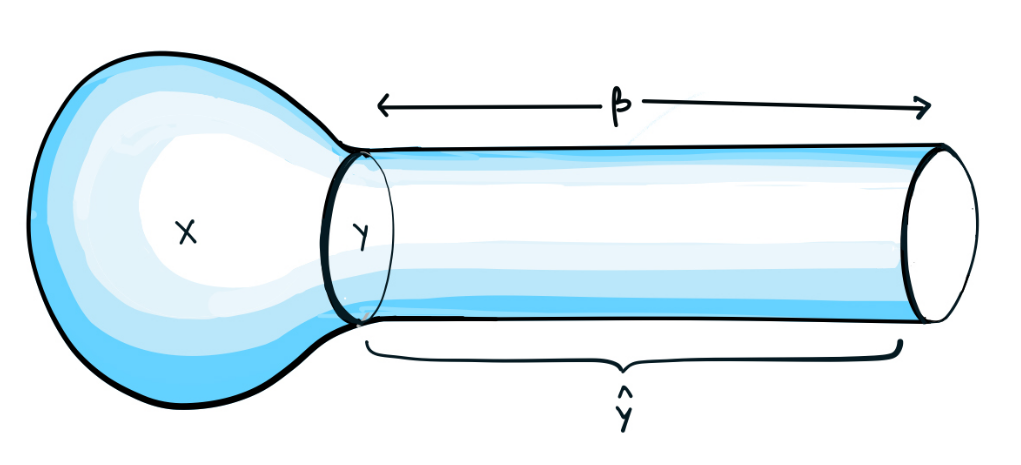
Figure 1: The extended manifold $\hat{X}$ obtained by attaching the cylinder $\hat{Y}=Y\times[0,\beta]$ to the boundary $Y$ of original manifold $X$.

On the other hand, we can interpret the correlation function in Eq. 32 as a path integral on a manifold $\hat{X}$ defined as follows. We first write the expectation value as

$$\langle\Omega|e^{i\alpha_{0}Q}|X,\mathcal{O}\rangle=\langle\Omega|e^{-\beta H}e^{i\alpha_{0}Q}|X,\mathcal{O}\rangle.$$ (34)

where we have assumed that the ground state energy vanishes for simplicity. The expression on the right hand side can be interpreted as a path integral on a manifold $\hat{X}$ which is defined by attaching a cylinder $Y\times[0,\beta]$ with the product metric to the boundary $Y$ of $X$, as shown in Fig. 1. Thus,

$$\langle\Omega|e^{-\beta H}e^{i\alpha_{0}\int_{Y}J}|X,\mathcal{O}\rangle =\langle e^{i\alpha_{0}\int_{Y}J}\mathcal{O}(x_{0})\rangle_{\hat{X}}$$

$$=\int[d\bar{\Psi}][d\Psi]e^{-S_{\hat{X}}}e^{i\alpha_{0}\int_{Y}J}\mathcal{O}(x_{0}),$$ (35)

where the fields are taken to live on $\hat{X}$ and $J$ is the chiral symmetry current. If we now perform the change of variables given in Eq. 28 with $\alpha(x)$ equal to $\alpha_{0}$ on $X$ and $0$ on $\hat{Y}$, then according to Eq. 29, the change in the measure is given by

$$[d\bar{\Psi}][d\Psi]\to[d\bar{\Psi}][d\Psi]e^{-2i\int_{\hat{X}}\alpha G}=[d\bar{\Psi}][d\Psi]e^{-2i\alpha_{0}\int_{X}G}.$$ (36)

We also have a change in the action given by

$$S\to S+i\int_{\hat{X}}d\alpha\wedge J=S+i\alpha_{0}\int_{Y}J,$$ (37)

where the last expression comes from the fact that $d\alpha$ is a delta function 1-form supported on $Y$. Finally, we have a change in $\mathcal{O}(x_{0})$ given by

$$\mathcal{O}(x_{0})\to e^{2i\alpha_{0}I}\mathcal{O}(x_{0}).$$ (38)

So with this change of variables, the right-hand side of Eq. 35 can be rewritten as

$$\langle\Omega|e^{-\beta H}e^{i\alpha_{0}\int_{Y}J}|X,\mathcal{O}\rangle$$

$$\quad=\int[d\bar{\Psi}][d\Psi]e^{-S}\mathcal{O}(x_{0})\ e^{2i\alpha_{0}I-2i\alpha_{0}\int_{X}G}$$

$$\quad=\langle\Omega|X,\mathcal{O}\rangle\ e^{2i\alpha_{0}I-2i\alpha_{0}\int_{X}G}.$$ (39)

Comparing Eqs. 33 and 39, we finally obtain

$$I=\int_{X}G+\frac{1}{2}\eta,$$ (40)

which is precisely the aps index theorem for kd fermions.

At this point, we can now comment on the aps index theorems for the two chiral symmetries. For the untwisted chiral symmetry, we obtain the Hirzebruch signature theorem on manifolds with boundary: $I$ is the signature, $G$ is the Hirzebruch $L$-polynomial, and the $\eta$ invariant gives a contribution from the boundary. On the other hand, in the case of the twisted chiral symmetry $\Gamma_{\chi}$, the index is the Euler characteristic and $G$ is the Euler density. However, as noted at the end of Sec. IV.1, the twisted chiral charge of the massless vacuum vanishes due the pairing of positive and negative eigenmodes. Therefore, the aps index theorem in this case is just the cgb theorem $\chi(X)=\int e(X)$, with $e(X)$ being the Euler density of the manifold $X$. In the usual presentation of the cgb theorem, there is an additional contribution from the geodesic curvature of $Y$ embedded in $X$. However, the requirement of product structure near the boundary implies that the geodesic curvature vanishes.

V Local, symmetric boundary conditions

The fact that there is no boundary contribution for the cgb theorem was noted in the motivation of the original work of aps [29]. For the twisted chiral symmetry, the obstruction to finding suitable symmetric, local, self-adjoint boundary conditions for the kd operator vanishes, while for the untwisted chiral symmetry, it does not.

To gain some understanding of the difference between to the two cases, let us consider for simplicity a local boundary condition of the form

$$L(\Phi|_{Y})=A(\Phi|_{Y})B=+\Phi|_{Y}.$$ (41)

for some matrices $A$ and $B$. In general, we require that $L^{2}=1$ (and hence $A^{2}=B^{2}=1$), and that the $L=+1$ and $L=-1$ eigenspaces have the same dimensions so that the boundary condition eliminates half of the modes. Another general requirement is ellipticity, which we will comment on below. But first, let us address what constraints on $A,B$ are needed in order for the kd operator to be self-adjoint or symmetric.

Self-adjointness and symmetries

In order to have $\mathcal{K}$ self-adjoint, the boundary condition must force the vanishing of the boundary term

$$\Delta =\int_{Y}d^{d}y\sqrt{h}\operatorname{tr}[\Psi^{\dagger}\gamma^{\tau}\Phi]$$

$$=\int_{Y}d^{d}y\sqrt{h}\operatorname{tr}[L(\Psi)^{\dagger}\gamma^{\tau}L(\Phi)].$$ (42)

We see that it suffices to take $L$ to be unitary and to anticommute with $\gamma^{\tau}$. In the case of the local boundary condition (41), this means

$$AA^{\dagger}=BB^{\dagger}=1,$$ (43)

$$A^{\dagger}\gamma^{\tau}A=-\gamma^{\tau}.$$ (44)

For the boundary condition to preserve a symmetry, $L$ must commute with the symmetry transformation. Let us see how this may be achieved for the local boundary condition (41). Consider first rotation invariance along the boundary. For this, we require $A,B$ to commute with the rotation generators $\sigma_{ab}$ with $a,b$ along the boundary. The most general choice of $A$ or $B$ which commutes with the $\sigma_{ab}$ are linear combinations of the form

$$A,B=a+b\gamma^{\tau}+c\bar{\gamma}+di\bar{\gamma}\gamma^{\tau}.$$ (45)

Next, let us look at the two chiral symmetries. To preserve untwisted-chiral symmetry, we need $[A,\bar{\gamma}]=0$, while $B$ can be arbitrary. We only have the choices $A=\mathbb{I},\bar{\gamma}$.

To preserve twisted-chiral symmetry, we need both $A,B$ to either commute or anticommute with $\bar{\gamma}$. For the commuting case, we can have

$$(A,B)=(\bar{\gamma},1),\,(\bar{\gamma},\bar{\gamma}),\,(1,\bar{\gamma}),$$ (46)

which will also preserve untwisted-chiral symmetry. For the anticommuting case, we can have

$$A,B =i\bar{\gamma}e^{{i\theta\bar{\gamma}}}\gamma^{\tau},$$ (47)

where $\theta{}$ may be different for $A$ and $B$. Note however that this will not preserve untwisted chiral symmetry. The analog of this for Dirac fermions (where $B$ plays no role) has been called “Euclidean (complex) chiral-bag” boundary conditions [63, 64, 65, 66, 67], which also does not preserve chiral symmetry. We shall refer to the boundary condition of Eq. 47 as the “twisted” chiral-bag boundary condition.

Comparing with Eqs. 43 and 44, we note that the twisted chiral-bag boundary condition is only self-adjoint for $\theta=0$. The case of $\theta=\pm\pi/2$, while not self-adjoint, is also of interest. The analog of it for Dirac fermions was considered in Ref. [27], so we call it the twisted Witten-Yonekura (wy) boundary condition.

At this point, it seems that a choice such as $A=\bar{\gamma}$, $B=1$ consistent with Eq. 46 has the virtues of ensuring self-adjointness of the Dirac operator [since it satisfies Eqs. 43 and 44] and of preserving both chiral symmetries. But it turns out to be unacceptable for a different reason – it is not elliptic.

Ellipticity

In order for a boundary condition to even be sensible, it must be elliptic. This means the following. We take $X=Y\times\mathbb{R}^{+}$ with $Y=\mathbb{R}^{d}$. We ask whether there are any normalizable zero-modes of $\mathcal{K}_{X}=i\gamma^{\mu}\partial_{\mu}$ satisfying the boundary condition $L$. If no solution exists, then we say the boundary condition is (strongly) elliptic.

Let us now determine when the boundary condition is elliptic. With the ansatz $\Psi(x,\tau)=\Phi(x)e^{-\lambda\tau}$, the equation for a zero mode $\mathcal{K}_{X}\Psi=0$ becomes

$$\mathcal{K}_{Y}\Phi=\lambda\Phi\quad(\lambda>0).$$ (48)

Now, if the operator $L$ commutes with $\mathcal{K}_{Y}$, then $\mathcal{K}_{Y}$ and $L$ can be simultaneously diagonalized. Moreover, if $L$ is local then for each $\lambda>0$ in the spectrum of $\mathcal{K}_{Y}$, there is a normalizable zero mode of $\mathcal{K}_{X}$ with $L=+1$. In the continuum limit, this means that there are infinitely many zero modes localized to the wall with arbitrarily high momenta along the boundary. This does not lead to a well-defined $(d+1)$-dimensional Euclidean field theory.

On the other hand, if $L$ anticommutes with $\mathcal{K}_{Y}$, then $L\Phi$ is an eigenstate of $\mathcal{K}_{Y}$ with eigenvalue $-\lambda$. Since $\lambda$ is nonzero, it follows that $L\Phi\neq\Phi$. Therefore, there is no solution with $\lambda>0$ which satisfies the boundary condition $L$. Such a boundary condition is therefore elliptic.

Clearly, the boundary condition in Eq. 46 commutes with $\mathcal{K}_{Y}$ and is therefore not elliptic. On the other hand, the (twisted) chiral-bag boundary condition given in Eq. 47 anticommutes with $\mathcal{K}_{Y}$ and is therefore elliptic. Since ellipticity is a necessary condition for the Euclidean field theory to be well-defined [27], the twisted chiral-bag boundary condition is the only sensible choice. (See also Refs. [66, 68] for discussions of ellipticity of the chiral-bag boundary conditions.)

In the usual presentation for Dirac fermions, the chiral-bag boundary condition has been considered [67, 65, 69, 68, 70, 71]. But in that case, as for the untwisted chiral symmetry for kd fermions, it is local, self-adjoint, and elliptic, but breaks the bulk chiral symmetry. The surprising fact here is that it has a twisted version, which preserves the twisted chiral symmetry. This lets us define a bulk index even in the presence of a boundary. This is completely consistent with the fact that the Euler characteristic can be defined for manifolds with a boundary. In fact, for the untwisted chiral symmetry there is no such local boundary condition, which necessitates the use of the nonlocal aps boundary conditions.

With the twisted chiral-bag boundary condition, one can proceed with the derivation of aps index theorem as in the previous section. Since the boundary-condition is local and symmetric, the twisted chiral charge of the boundary state vanishes, and there is no contribution from the boundary $\eta$ invariant. This is another way to understand the result derived earlier about there being no boundary contribution to the cgb theorem.

Before closing, we note that the nonlocal aps boundary conditions can be easily seen to be self-adjoint, symmetric and elliptic. Using the expression $L=-\varepsilon(\mathcal{K}_{Y})$ from Eq. 22, it is clear that $L$ is unitary and anticommutes with $\gamma^{\tau}$, and is therefore self-adjoint [see Eq. 42]. It also commutes with $\bar{\gamma}$, so preserves (both notions of) bulk chirality. Finally, ellipticity: as discussed earlier, a normalizable zero-mode of $\mathcal{K}_{X}$ corresponds to a solution of Eq. 48 with $\lambda>0$. But these are exactly the modes killed by the aps boundary condition $L=+1$. Therefore, the aps boundary condition is elliptic.

VI Conclusion

Recently, kd fermions have found applications in attempts to use smg as an ingredient of chiral lattice gauge theories, as well as in explaining the classification of bosonic spt phases. This is because kd fermions have a natural lattice discretization which preserves many features of the continnum, including some ’t Hooft anomalies. On the other hand, the aps index theorem has been recognized as an important ingredient in obtaining a nonperturbative picture of anomaly cancellation for fermionic theories. Motivated by these connections, in this work, we derive the aps index theorem using a “physics” approach due to Ref. [56], which generalizes Fujikawa’s method to manifolds with boundary. In this approach, the connection to anomaly inflow is manifest – the boundary state may be charged under the chiral symmetry, and this causes an additional contribution to the usual as index theorem from the boundary. This extra contribution is precisely the $\eta$ invariant of the boundary Dirac operator.

An interesting feature of kd fermions, which distinguishes them from Dirac fermions, is that there are two notions of a chiral symmetry. In flat space, where kd fermions can be decomposed into $2^{{D/2}}$ Dirac flavors, one of them corresponds to the usual chiral symmetry $\Gamma_{\sigma}$ and other symmetry $\Gamma_{\chi}$ corresponds to a mixed chiral–flavor transformation, hence the name “twisted” chiral symmetry. Both of these have a perturbative mixed anomaly with gravity, and therefore lead to index theorems via Fujikawa’s method. It is known that (for example, see Ref.  [61]) the index theorems for the twisted- and untwisted-chiral symmetries correspond to the Chern-Gauss-Bonnet and Hirzebruch signature theorems, respectively.

When trying to generalize the as index theorem to manifolds with boundary, it is important to choose the boundary conditions carefully. It was noted by aps [29] that the attempt to extend Hirzebruch signature theorem to manifolds with boundary meets with an obstruction to finding sensible local boundary conditions. Therefore, in trying to define an index, one is forced to consider the nonlocal aps boundary conditions. These boundary conditions have a natural interpretation as those corresponding to a massless fermion ground state at the boundary [32], and the $\eta$ invariant appears as the chiral charge of this boundary state for the Hirzebruch theorem. On the other hand, for the cgb theorem, we find that the boundary charge vanishes for the aps state. This is why there is no contribution from the boundary $\eta$ invariant for the index theorem associated with the twisted chiral symmetry.

The fact that there is no boundary correction to the cgb theorem can also be understood in another way. If we can find a “good” local and symmetric boundary, which corresponds to some state in the boundary fermion Hilbert space, then we could use that instead of the aps state in our proof, and the charge would trivially vanish. We found that such a boundary condition can in fact be defined. In the context of Dirac fermions, these boundary conditions have been called Euclidean chiral-bag boundary conditions. However, an important difference from the case of Dirac fermions (and untwisted chiral symmetry for kd fermions) is that the chiral-bag boundary conditions are not chirally symmetric in that case, while the twisted boundary conditions are. The existence of such local, symmetric boundary conditions for twisted chiral symmetry is consistent with the fact that the Euler characteristic can be defined for manifolds with boundary with no problem.

Recently, Catterall [15] has argued that the problem of chiral fermions has an analog for kd fermions. Using the twisted-chiral symmetry allows one to solve this problem. This is due to the “onsite” nature of the twisted-chiral symmetry on the lattice, which plays an important role in demonstrating anomaly cancellation on the lattice. In line with this, there has been a significant improvement in the understanding of how anomalies can arise on the lattice with onsite symmetries [72, 54, 73, 74, 75, 76]. This onsite nature of the twisted symmetry makes the analogous problem of chiral lattice gauge theory much more tractable [15] than Lüscher’s approach where one needs to define a nonlocal $\gamma_{5}$ matrix using gw fermions [77, 7, 8, 78]. In the genuinely difficult case of (untwisted) chiral symmetry where there is no known onsite lattice discretization, one has to gauge non-onsite symmetries [8, 79, 76]. As we have argued, the twisted-chiral symmetry is also special from another perspetive in that there is no obstruction to formulating a symmetric, local boundary condition, and therefore the aps index theorem has no boundary contribution from the $\eta$ invariant. This might provide another way to understand the role played by twisted-chiral symmetry in this problem. This is also interesting in light of Kaplan’s recent proposal [17, 16] with a single domain-wall where the role of the aps index theorem is manifest. A lattice version of the aps index theorem may help tie the various approaches together. (For example, see also Refs. [80, 81] for an approach to formulating the aps index theorem on the lattice which uses domain-wall fermions.) This is likely to be important in understanding the problem of formulating chiral gauge theory on the lattice.

Appendix A Review of differential forms

Differential $p$-forms are totally antisymmetric covariant tensor fields with $p$ indices, $\phi_{\mu_{1}\ldots\mu_{p}}$. A coordinate invariant way to express these objects is to introduce totally antisymmetric products of coordinate differentials $dx^{\mu_{1}}\wedge\cdots\wedge dx^{\mu_{p}}$ and write

$$\phi^{(p)}=\frac{1}{p!}\phi_{\mu_{1}\ldots\mu_{p}}dx^{\mu_{1}}\wedge\cdots\wedge dx^{\mu_{p}},$$ (49)

The product of differential forms $\phi^{(p)}\wedge\psi^{(q)}$ is then defined in the obvious way.

A natural derivative of differential forms is the exterior derivative $d$, defined by

$$d\phi^{(p)}=dx^{\mu}\wedge\partial_{\mu}\phi^{(p)}.$$ (50)

This derivative is clearly coordinate invariant and independent of the metric. A crucial property is nilpotency: $d^{2}=0$.

Another important operation on differential forms, available when the manifold has a metric $g_{\mu\nu}$, is the Hodge star operation $\star$ which transforms a $p$-form into a $(D-p)$-form. In components, it is defined by

$$(\star\phi)_{\mu_{p+1}\ldots\mu_{D}}=\frac{1}{p!}\sqrt{g}\epsilon_{\mu_{1}\ldots\mu_{p}\mu_{p+1}\ldots\mu_{D}}\phi^{\mu_{1}\ldots\mu_{p}},$$ (51)

where $\epsilon_{\mu_{1}\ldots\mu_{D}}$ is totally antisymmetric Levi-Cevita symbol. It is straightforward to show that

$$\star^{2}=(-1)^{p(D-p)}$$ (52)

on $p$-forms.

With the help of the Hodge star, an inner product on the space of $p$-forms can be defined by

$$(\psi^{(p)},\phi^{(p)}) =\int\psi^{(p)*}\wedge{\star\phi^{(p)}}$$

$$=\frac{1}{p!}\int\psi^{*}_{\mu_{1}\ldots\mu_{p}}\phi^{\mu_{1}\ldots\mu_{p}}\sqrt{g}d^{D}x,$$ (53)

where in the last expression indices are raised with the metric tensor.

Given this inner product structure, there is another natural derivative $\delta$, defined as the formal adjoint of $d$:

$$(\psi^{(p)},d\phi^{(p-1)})=(\delta\psi^{(p)},\phi^{(p-1)}).$$ (54)

It is straightforward to express $\delta$ in terms of the exterior derivative and the Hodge star:

$$\delta=(-1)^{p}\star^{-1}d\star$$ (55)

on $p$-forms. Note that the nilpotency of $d$ also implies the nilpotency of $\delta$.

The Laplacian of arbitrary differential forms is given by

$$\Delta=d\delta+\delta d.$$ (56)

The Kähler-Dirac operator is a square-root of this Laplacian:

$$\mathcal{K}=i(d-\delta).$$ (57)

Note that it does not require a spin structure to be defined.

Appendix B Review of vielbeins

An orthonormal frame (or “vielbein”) is a collection of $D$ orthonormal vector fields $e_{m\mu}$ ($m=1,\ldots,D$):

$$g^{\mu\nu}e_{m\mu}e_{n\nu}=\delta_{mn}.$$ (58)

The orthonormality of the frame also implies the completeness relation

$$e_{m\mu}e_{m\nu}=g_{\mu\nu}.$$ (59)

(Summation over repeated Latin indices is understood.) Here, we are adopting an index convention where Greek indices $\mu,\nu,\ldots$ are “curved space” indices, while Latin indices $m,n,\ldots$ are “flat space” indices, which simply label the various vectors in the frame.

If we have matrices $\gamma_{m}$ that satisfy the flat space Clifford algebra

$$\{\gamma_{m},\gamma_{n}\}=2\delta_{mn},$$ (60)

then the matrices $\Gamma_{\mu}\equiv\gamma_{m}e_{m\mu}$ will satisfy the curved space Clifford algebra

$$\{\Gamma_{\mu},\Gamma_{\nu}\}=2g_{\mu\nu}.$$ (61)

Under a frame rotation

$$e_{m\mu}\to e_{n\mu}R_{nm},$$ (62)

where $R_{mn}$ is a matrix in $SO(D)$, the curved space gamma matrices transform as

$$\Gamma_{\mu}\to S^{-1}(R)\Gamma_{\mu}S(R),$$ (63)

where $S(R)$ is a lift of $R$ to the spin group $\mathrm{Spin}(D)$. The matrix representation of the kd field, $\Phi$, transforms in the same way under such a frame rotation:

$$\Phi\to S^{-1}(R)\Phi S(R).$$ (64)

Note that the sign ambiguity in choosing the lift $S(R)$ cancels out in these transformation laws. This of course reflects the fact that no spin structure is required to define kd fields on arbitrary manifolds.

We can define a covariant derivative for kd fields by

$$D_{\mu}\Phi=\partial_{\mu}\Phi+\tfrac{1}{2}\omega_{mn\mu}[\sigma_{mn},\Phi].$$ (65)

Here, $\omega_{mn\mu}$ is the spin connection, defined by

$$\nabla_{\mu}e_{n\nu}=e_{m\nu}\omega_{mn\mu},$$ (66)

where $\nabla_{\mu}$ is the ordinary Levi-Cevita derivative operator; and the $\sigma_{mn}$ are the generators of $\mathrm{Spin}(D)$:

$$\sigma_{mn}=\tfrac{1}{4}[\gamma_{m},\gamma_{n}].$$ (67)

The kd operator can then be written as $\mathcal{K}=i\Gamma^{\mu}D_{\mu}$.

With the help of the product rule

$$\nabla_{\mu}\operatorname{tr}\Psi^{\dagger}\Gamma^{\mu}\Phi=\operatorname{tr}[(D_{\mu}\Psi)^{\dagger}\Gamma^{\mu}\Phi+\Psi^{\dagger}\Gamma^{\mu}D_{\mu}\Phi],$$ (68)

we see that on closed manifolds, Hermiticity of the kd operator is manifest, while on manifolds with boundary, Hermiticity requires the vanishing of the boundary term

$$\Delta=\int_{Y}d^{d}y\sqrt{h}\operatorname{tr}\Psi^{\dagger}\gamma^{\tau}\Phi.$$ (69)

Boundary conditions that ensure $\Delta=0$ are discussed in the main text.

Appendix C Untwisted chiral symmetry

In this appendix, we derive the form of the chirality operator $\Gamma=\Gamma_{\sigma}$ that exchanges $d$ and $\delta$.

The formula $\delta=(-1)^{k}\star^{-1}d\star$, where $\star$ is the Hodge star operation on forms (Appendix A), suggests the ansatz $\Gamma_{\sigma}=\star B$ where $B$ acts as degree-dependent phase factor. Writing $B=B_{k}$ for the action of $B$ on $k$-forms, the requirement that $\Gamma_{\sigma}$ exchange $d$ and $\delta$ gives

$$\delta =\Gamma_{\sigma}^{-1}d\Gamma_{\sigma}$$

$$=B^{-1}(\star^{-1}d\star)B$$

$$=(-1)^{k}B^{-1}\delta B$$

$$=(-1)^{k}\frac{B_{k}}{B_{k-1}}\delta.$$ (70)

This gives the recursion relation $B_{k}=(-1)^{k}B_{k-1}$, which can be solved to give $B_{k}=(-1)^{g_{k}}B_{0}$, where $g_{k}=\frac{1}{2}k(k+1)$. On the other hand, the requirement that $\Gamma_{\sigma}$ square to the identity gives

$$1 =\Gamma_{\sigma}^{2}$$

$$=B_{D-k}B_{k}(-1)^{k(D-k)}$$

$$=(B_{0})^{2}(-1)^{g_{D-k}+g_{k}+k(D-k)}$$

$$=(B_{0})^{2}(-1)^{g_{D}}.$$ (71)

where in the second line we have used the fact $\star^{2}=(-1)^{k(D-k)}$ on $k$-forms. Therefore, we can choose $B_{0}=(\pm i)^{g_{D}}$, which finally gives

$$B_{k}=(-1)^{g_{k}}(\pm i)^{g_{D}}.$$ (72)

The overall sign $(\pm 1)^{g_{D}}$ may be chosen arbitrarily. The operator $B$ is referred to as the main anti-automorphism in Ref. [49].

References

- Nielsen and Ninomiya [1981] H. B. Nielsen and M. Ninomiya, Absence of Neutrinos on a Lattice. 1. Proof by Homotopy Theory, Nucl. Phys. B 185, 20 (1981), [Erratum: Nucl.Phys.B 195, 541 (1982)].
- Ginsparg and Wilson [1982] P. H. Ginsparg and K. G. Wilson, A Remnant of Chiral Symmetry on the Lattice, Phys. Rev. D 25, 2649 (1982).
- Kaplan [1992] D. B. Kaplan, A method for simulating chiral fermions on the lattice, Phys. Lett. B 288, 342 (1992), arXiv:hep-lat/9206013 .
- Narayanan and Neuberger [1993] R. Narayanan and H. Neuberger, Chiral fermions on the lattice, Phys. Rev. Lett. 71, 3251 (1993), arXiv:hep-lat/9308011 .
- Shamir [1993] Y. Shamir, Chiral fermions from lattice boundaries, Nuclear Physics B 406, 90 (1993).
- Neuberger [1998] H. Neuberger, Exactly massless quarks on the lattice, Phys. Lett. B 417, 141 (1998), arXiv:hep-lat/9707022 .
- Lüscher [2001] M. Lüscher, Chiral gauge theories revisited, Theory and Experiment Heading for New Physics; World Scientific: Singapore , 41 (2001), arXiv:hep-th/0102028 .
- Lüscher [1999] M. Lüscher, Abelian chiral gauge theories on the lattice with exact gauge invariance, Nuclear Physics B 549, 295 (1999).
- Kikukawa [2002] Y. Kikukawa, Domain wall fermion and chiral gauge theories on the lattice with exact gauge invariance, Physical Review D 65, 074504 (2002), arxiv:hep-lat/0105032 .
- Kaplan [2012] D. B. Kaplan, Chiral Symmetry and Lattice Fermions (2012), arxiv:0912.2560 [hep-lat, physics:hep-ph, physics:hep-th] .
- Aoki et al. [2024a] S. Aoki, H. Fukaya, and N. Kan, A lattice regularization of Weyl fermions in a gravitational background (2024a), arxiv:2401.05636 [cond-mat, physics:hep-lat, physics:hep-th] .
- Aoki et al. [2024b] S. Aoki, H. Fukaya, and N. Kan, A lattice formulation of Weyl fermions on a single curved surface (2024b), arxiv:2402.09774 [cond-mat, physics:hep-lat, physics:hep-th] .
- Berkowitz et al. [2023] E. Berkowitz, A. Cherman, and T. Jacobson, Exact lattice chiral symmetry in 2d gauge theory (2023), arxiv:2310.17539 [hep-lat, physics:hep-th] .
- Catterall [2021] S. Catterall, Chiral lattice fermions from staggered fields, Physical Review D 104, 014503 (2021).
- Catterall [2023] S. Catterall, Lattice Regularization of Reduced K\”{a}hler-Dirac Fermions and Connections to Chiral Fermions (2023), arxiv:2311.02487 [hep-lat, physics:hep-th] .
- Kaplan [2024] D. B. Kaplan, Chiral gauge theory at the boundary between topological phases (2024), arxiv:2312.01494 [cond-mat, physics:hep-lat, physics:hep-th] .
- Kaplan and Sen [2024] D. B. Kaplan and S. Sen, Weyl fermions on a finite lattice (2024), arxiv:2312.04012 [cond-mat, physics:hep-lat, physics:hep-th] .
- Pedersen and Kikukawa [2023] J. W. Pedersen and Y. Kikukawa, Reformulation of anomaly inflow on the lattice and construction of lattice chiral gauge theories, PoS LATTICE2022, 381 (2023).
- Wang and Wen [2022] J. Wang and X.-G. Wen, Non-Perturbative Regularization of 1+1D Anomaly-Free Chiral Fermions and Bosons: On the equivalence of anomaly matching conditions and boundary gapping rules (2022), arxiv:1307.7480 .
- Wang and Wen [2019] J. Wang and X.-G. Wen, Solution to the $1+1$ dimensional gauged chiral Fermion problem, Physical Review D 99, 111501 (2019).
- Wang and You [2022] J. Wang and Y.-Z. You, Symmetric Mass Generation, Symmetry 14, 1475 (2022), arxiv:2204.14271 [cond-mat, physics:hep-lat, physics:hep-ph, physics:hep-th, physics:quant-ph] .
- Zeng et al. [2022] M. Zeng, Z. Zhu, J. Wang, and Y.-Z. You, Symmetric Mass Generation in the $1+1$ Dimensional Chiral Fermion 3-4-5-0 Model, Physical Review Letters 128, 185301 (2022).
- Golterman and Shamir [2024a] M. Golterman and Y. Shamir, Conserved currents in five-dimensional proposals for lattice chiral gauge theories (2024a), arxiv:2404.16372 [hep-lat, physics:hep-th] .
- Golterman and Shamir [2024b] M. Golterman and Y. Shamir, Propagator Zeros and Lattice Chiral Gauge Theories, Physical Review Letters 132, 081903 (2024b).
- Clancy et al. [2024] M. Clancy, D. B. Kaplan, and H. Singh, Generalized Ginsparg-Wilson relations, Phys. Rev. D 109, 014502 (2024).
- Callan and Harvey [1985] C. G. Callan, Jr. and J. A. Harvey, Anomalies and fermion zero modes on strings and domain walls, Nucl. Phys. B 250, 427 (1985).
- Witten and Yonekura [2020] E. Witten and K. Yonekura, Anomaly Inflow and the -Invariant (2020), arXiv:1909.08775 .
- Witten [2016] E. Witten, Fermion path integrals and topological phases, Reviews of Modern Physics 88, 035001 (2016), arXiv:1508.04715 .
- Atiyah et al. [1975] M. F. Atiyah, V. K. Patodi, and I. M. Singer, Spectral asymmetry and Riemannian Geometry. I, Mathematical Proceedings of the Cambridge Philosophical Society 77, 43 (1975).
- Kapustin et al. [2015] A. Kapustin, R. Thorngren, A. Turzillo, and Z. Wang, Fermionic Symmetry Protected Topological Phases and Cobordisms, Journal of High Energy Physics 2015, 1 (2015), arxiv:1406.7329 [cond-mat, physics:hep-th] .
- Dai and Freed [1994] X. Dai and D. S. Freed, -invariants and determinant lines, Journal of Mathematical Physics 35, 5155 (1994), arXiv:hep-th/9405012 .
- Yonekura [2016] K. Yonekura, Dai-Freed theorem and topological phases of matter, Journal of High Energy Physics 2016, 22 (2016).
- García-Etxebarria and Montero [2019] I. García-Etxebarria and M. Montero, Dai-Freed anomalies in particle physics, Journal of High Energy Physics 2019, 3 (2019).
- Eichten and Preskill [1986] E. Eichten and J. Preskill, Chiral gauge theories on the lattice, Nuclear Physics B 268, 179 (1986).
- Ayyar and Chandrasekharan [2016a] V. Ayyar and S. Chandrasekharan, Fermion masses through four-fermion condensates, Journal of High Energy Physics 2016, 58 (2016a).
- Ayyar and Chandrasekharan [2017] V. Ayyar and S. Chandrasekharan, Generating a nonperturbative mass gap using Feynman diagrams in an asymptotically free theory, Physical Review D 96, 114506 (2017).
- Ayyar and Chandrasekharan [2016b] V. Ayyar and S. Chandrasekharan, Origin of fermion masses without spontaneous symmetry breaking, Physical Review D 93, 081701 (2016b).
- Catterall and Butt [2018] S. Catterall and N. Butt, Topology and strong four fermion interactions in four dimensions, Physical Review D 97, 094502 (2018).
- Razamat and Tong [2021] S. S. Razamat and D. Tong, Gapped Chiral Fermions, Physical Review X 11, 011063 (2021), arxiv:2009.05037 [cond-mat, physics:hep-ph, physics:hep-th] .
- You and Xu [2015] Y.-Z. You and C. Xu, Interacting topological insulator and emergent grand unified theory, Physical Review B 91, 125147 (2015).
- Butt et al. [2021] N. Butt, S. Catterall, A. Pradhan, and G. C. Toga, Anomalies and symmetric mass generation for K\”ahler-Dirac fermions, Physical Review D 104, 094504 (2021).
- Catterall et al. [2018] S. Catterall, J. Laiho, and J. Unmuth-Yockey, Topological fermion condensates from anomalies, Journal of High Energy Physics 2018, 13 (2018).
- Butt et al. [2018] N. Butt, S. Catterall, and D. Schaich, $SO(4)$ invariant Higgs-Yukawa model with reduced staggered fermions, Physical Review D 98, 114514 (2018), arxiv:1810.06117 [cond-mat, physics:hep-lat, physics:hep-th] .
- Creutz et al. [1997] M. Creutz, M. Tytgat, C. Rebbi, and S.-S. Xue, Lattice Formulation of the Standard Model, Physics Letters B 402, 341 (1997), arxiv:hep-lat/9612017 .
- Kikukawa [2019] Y. Kikukawa, Why is the mission impossible? – Decoupling the mirror Ginsparg-Wilson fermions in the lattice models for two-dimensional abelian chiral gauge theories, Progress of Theoretical and Experimental Physics 2019, 073B02 (2019), arxiv:1710.11101 [hep-lat] .
- Poppitz and Shang [2007] E. Poppitz and Y. Shang, Lattice chirality and the decoupling of mirror fermions, Journal of High Energy Physics 2007, 081 (2007), arxiv:0706.1043 [hep-lat, physics:hep-th] .
- Kähler [1962] E. Kähler, Der innere Differentialkalkül, Abhandlungen aus dem Mathematischen Seminar der Universität Hamburg 25, 192 (1962).
- Banks et al. [1982] T. Banks, Y. Dothan, and D. Horn, Geometric fermions, Physics Letters B 117, 413 (1982).
- Becher and Joos [1982] P. Becher and H. Joos, The Dirac-Kähler equation and fermions on the lattice, Zeitschrift für Physik C Particles and Fields 15, 343 (1982).
- Rabin [1982] J. M. Rabin, Homology theory of lattice fermion doubling, Nuclear Physics B 201, 315 (1982).
- Susskind [1977] L. Susskind, Lattice fermions, Physical Review D 16, 3031 (1977).
- Sharatchandra et al. [1981] H. S. Sharatchandra, H. J. Thun, and P. Weisz, Susskind fermions on a euclidean lattice, Nuclear Physics B 192, 205 (1981).
- Catterall et al. [2009] S. Catterall, D. B. Kaplan, and M. Ünsal, Exact lattice supersymmetry, Physics Reports 484, 71 (2009).
- Catterall [2022] S. Catterall, ’t Hooft anomalies for staggered fermions (2022), arxiv:2209.03828 [cond-mat, physics:hep-lat, physics:hep-th] .
- Guo and You [2023] Y. Guo and Y.-Z. You, Symmetric Mass Generation of K\”ahler-Dirac Fermions from the Perspective of Symmetry-Protected Topological Phases (2023), arxiv:2306.17420 [cond-mat] .
- Kobayashi and Yonekura [2021] S. K. Kobayashi and K. Yonekura, Atiyah-Patodi-Singer index theorem from axial anomaly, Progress of Theoretical and Experimental Physics 2021, 073B01 (2021), arxiv:2103.10654 [cond-mat, physics:hep-th] .
- Fujikawa [1979] K. Fujikawa, Path-integral measure for gauge-invariant fermion theories, Physical Review Letters 42, 1195 (1979).
- Göckeler [1983] M. Göckeler, Axial-vector anomaly for Dirac-Kähler fermions on the lattice, Nuclear Physics B 224, 508 (1983).
- Linhares et al. [1985] C. A. Linhares, J. A. Mignaco, and M. A. Rego Monteiro, Axial anomaly and index theorem for Dirac-Kähler fermions, Letters in Mathematical Physics 10, 79 (1985).
- Shimono [1990] M. Shimono, Fermions and Gravitational Anomaly in Lattice Gravity, Progress of Theoretical Physics 84, 331 (1990).
- Green et al. [2012] M. B. Green, J. H. Schwarz, and E. Witten, Superstring Theory: Volume 2 (Cambridge University Press, 2012).
- Catterall and Pradhan [2022] S. Catterall and A. Pradhan, Induced topological gravity and anomaly inflow from K\”ahler-Dirac fermions in odd dimensions, Physical Review D 106, 014509 (2022).
- Hrasko and Balog [1984] P. Hrasko and J. Balog, The Fermion Boundary Condition and the theta Angle in QED in Two-dimensions, Nucl. Phys. B 245, 118 (1984).
- Wipf and Duerr [1995] A. Wipf and S. Duerr, Gauge Theories in a Bag, Nuclear Physics B 443, 201 (1995), arxiv:hep-th/9412018 .
- Chodos et al. [1974a] A. Chodos, R. L. Jaffe, K. Johnson, and C. B. Thorn, Baryon structure in the bag theory, Physical Review D 10, 2599 (1974a).
- Beneventano et al. [2003] C. G. Beneventano, P. B. Gilkey, K. Kirsten, and E. M. Santangelo, Strong ellipticity and spectral properties of chiral bag boundary conditions, J. Phys. A 36, 11533 (2003).
- Chodos et al. [1974b] A. Chodos, R. L. Jaffe, K. Johnson, C. B. Thorn, and V. F. Weisskopf, New extended model of hadrons, Physical Review D 9, 3471 (1974b).
- Ivanov and Vassilevich [2022] A. V. Ivanov and D. V. Vassilevich, Anomaly inflow for local boundary conditions, JHEP 09, 250.
- Kurkov and Vassilevich [2017] M. Kurkov and D. Vassilevich, Parity anomaly in four dimensions, Phys. Rev. D 96, 025011 (2017).
- Kurkov and Vassilevich [2018] M. Kurkov and D. Vassilevich, Gravitational parity anomaly with and without boundaries, Journal of High Energy Physics 2018, 72 (2018), arxiv:1801.02049 [gr-qc, physics:hep-th, physics:math-ph] .
- Fialkovsky et al. [2019] I. Fialkovsky, M. Kurkov, and D. Vassilevich, Quantum Dirac fermions in half space and their interaction with electromagnetic field, Physical Review D 100, 045026 (2019), arxiv:1906.06704 [cond-mat, physics:hep-th, physics:math-ph] .
- Nguyen and Singh [2023] M. Nguyen and H. Singh, Lattice regularizations of vacua: Anomalies and qubit models, Physical Review D 107, 014507 (2023).
- Cheng and Seiberg [2023] M. Cheng and N. Seiberg, Lieb-Schultz-Mattis, Luttinger, and ’t Hooft – anomaly matching in lattice systems, SciPost Physics 15, 051 (2023), arxiv:2211.12543 [cond-mat, physics:hep-th] .
- Fazza and Sulejmanpasic [2023] L. Fazza and T. Sulejmanpasic, Lattice quantum Villain Hamiltonians: Compact scalars, U(1) gauge theories, fracton models and quantum Ising model dualities, Journal of High Energy Physics 2023, 17 (2023).
- Gorantla et al. [2021] P. Gorantla, H. T. Lam, N. Seiberg, and S.-H. Shao, A Modified Villain Formulation of Fractons and Other Exotic Theories, Journal of Mathematical Physics 62, 102301 (2021), arxiv:2103.01257 [cond-mat, physics:hep-th] .
- Seifnashri [2024] S. Seifnashri, Lieb-Schultz-Mattis anomalies as obstructions to gauging (non-on-site) symmetries, SciPost Physics 16, 098 (2024), arxiv:2308.05151 [cond-mat, physics:hep-lat, physics:hep-th] .
- Lüscher [1998] M. Lüscher, Exact chiral symmetry on the lattice and the Ginsparg-Wilson relation, Phys. Lett. B 428, 342 (1998), arXiv:hep-lat/9802011 .
- Poppitz and Shang [2010] E. Poppitz and Y. Shang, Chiral Lattice Gauge Theories Via Mirror-Fermion Decoupling: A Mission (im)Possible?, Int. J. Mod. Phys. A 25, 2761 (2010).
- Catterall and Pradhan [2024] S. Catterall and A. Pradhan, Gauging staggered fermion shift symmetries and lattice anomalies (2024), arxiv:2405.03037 [hep-lat, physics:hep-th] .
- Fukaya et al. [2022] H. Fukaya, M. Furuta, Y. Matsuki, S. Matsuo, T. Onogi, S. Yamaguchi, and M. Yamashita, Mod-two APS index and domain-wall fermion, Lett. Math. Phys. 112, 16 (2022).
- Fukaya et al. [2020] H. Fukaya, N. Kawai, Y. Matsuki, M. Mori, K. Nakayama, T. Onogi, and S. Yamaguchi, The atiyah–patodi–singer index on a lattice, Progress of Theoretical and Experimental Physics 2020, 043B04 (2020), arXiv:1910.09675 .