Entanglement Entropy of Free Fermions with a Random Matrix as a One-Body Hamiltonian

Abstract

We consider a quantum system of large size $N$ and its subsystem of size $L$ assuming that $N$ is much larger than $L$, which can also be sufficiently large, i.e., $1\ll L\lesssim N$. A widely accepted mathematical version of this heuristic inequality is the asymptotic regime of successive limits: first the macroscopic limit $N\to\infty$, then an asymptotic analysis of the entanglement entropy as $L\to\infty$. In this paper, we consider another version of the above heuristic inequality: the regime of asymptotically proportional $L$ and $N$, i.e., the simultaneous limits $L\to\infty,\;N\to\infty,L/N\to\lambda>0$. Specifically, we consider the system of free fermions which is in its ground state and such that its one-body Hamiltonian is a large random matrix, that is often used to model the long-range hopping. By using random matrix theory, we show that in this case, the entanglement entropy obeys the volume law known for systems with short-ranged hopping but described either by a mixed state or a pure strongly excited state of the Hamiltonian. We also give a streamlined proof of Page’s formula for the entanglement entropy of the black hole radiation for a wide class of typical ground states, thereby proving the universality of the formula.

Keywords: entanglement; entanglement entropy; free fermions; area law; enhanced area law; volume law; random matrices

1 Introduction

Quantum entanglement, a special form of quantum correlation, is regarded as one of the important ingredients of modern quantum mechanics and adjacent fields of science and technology. In its simplest form, the entanglement causes two quantum objects (spins, qubits, etc.) to share a common pure state in which they do not have pure states of their own.

A general version of this simplest form is known as the bipartite setting where a quantum system $\mathfrak{S}$ consists of parties $\mathfrak{B}$ and $\mathfrak{E}$, i.e., symbolically

$$\mathfrak{S}=\mathfrak{B}\cup\mathfrak{E}.$$ (1.1)

Sometimes the parties are two communicating agents, sometimes one of them, say $\mathfrak{B}$ (block), is the system of interest while $\mathfrak{E}$ is the environment of $\mathfrak{B}$, etc. There is a variety of versions and models for this general setting and related problems, see e.g. [1, 2, 3, 4, 5, 6, 7, 8, 9, 10, 11, 12] for reviews.

Denote by $\mathcal{H}_{\mathfrak{S}}$, $\mathcal{H}_{\mathfrak{B}}$, and $\mathcal{H}_{\mathfrak{E}}$ the corresponding state spaces, so that

$$\mathcal{H}_{\mathfrak{S}}=\mathcal{H}_{\mathfrak{B}}\otimes\mathcal{H}_{\mathfrak{E}},$$ (1.2)

and by $\mathrm{tr}_{\mathfrak{B}}$ and $\mathrm{tr}_{\mathfrak{E}}$ the operation of (partial) traces in $\mathcal{H}_{\mathfrak{B}}$ and $\mathcal{H}_{\mathfrak{E}}$. Let $\rho_{\mathfrak{S}}$ be the density matrix of $\mathfrak{S}$, which is often assumed to be in a pure state, i.e.,

$$\rho_{\mathfrak{S}}=|\Psi_{\mathfrak{S}}\rangle\langle\Psi_{\mathfrak{S}}|.$$ (1.3)

Applying $\mathrm{tr}_{\mathfrak{E}}$ to $\rho_{\mathfrak{S}}$, we obtain the reduced density matrix

$$\rho_{\mathfrak{B}\mathfrak{S}}=\mathrm{tr}_{\mathfrak{E}}\,\rho_{\mathfrak{S}},\;\mathrm{tr}_{\mathfrak{B}}\,\rho_{\mathfrak{B}\mathfrak{S}}=1$$ (1.4)

of the $\mathfrak{B}$, a positive definite operator acting in $\mathcal{H}_{\mathfrak{B}}$. It can be viewed as quantum analog of the marginal distribution of probability theory.

If $\mathfrak{B}$ consists of several (1, 2, etc.) elementary objects, then the corresponding reduced density matrices are known in quantum statistical mechanics as the one-, two-, etc.-point correlation functions. In this paper we will deal with extended systems and their subsystems (parties), hence, with reduced density matrices (correlation functions) of large size.

One of widely used numerical characteristics (quantifiers) of the quantum correlations between the parties is the entanglement is entropy

$$S_{\mathfrak{B}\mathfrak{S}}=-\mathrm{tr}_{\mathfrak{B}}\rho_{\mathfrak{B}}\log_{2}\rho_{\mathfrak{B}\mathfrak{S}},$$ (1.5)

i.e., the von Neumann entropy of the reduced density matrix (1.4).

Let $\Omega$ and $\Lambda\subset\Omega$ be the spatial domains occupied by $\mathfrak{S}$ and $\mathfrak{B}$ and $N$ and $L$ be the parameters determining the size of $\mathfrak{S}$ and $\mathfrak{B}$ (e.g. the corresponding side lengths if $\Omega$ is a cube in $\mathbb{R}^{d}$ and $\Lambda$ is a sub-cube, so that $|\Omega|=N^{d}$ and $|\Lambda|=L^{d}$). We will assume that

$$1\ll L\lesssim N,$$ (1.6)

i.e., that $\mathfrak{E}$ (an "environment") is much larger than $\mathfrak{B}$ (block) which can also be sufficiently large.

The goal is to find the asymptotic form of $S_{\mathfrak{B}}$ in a certain formalization of the heuristic inequalities (1.6).

Then the most widely used formalization of (1.6) is as follows. The r.h.s. of (1.6) is implemented in its strong form $L\ll$ N via the macroscopic limit $N\rightarrow\infty$ for $\mathfrak{S}$ in (1.1) keeping $L$ fixed under a condition guarantying the existence of a well defined limiting entanglement entropy

$$S_{\mathfrak{B}}=\lim_{N\to\infty}S_{\mathfrak{B}\mathfrak{S}}.$$ (1.7)

Then the l.h.s. $1\ll L$ of (1.6) is implemented as the asymptotic regime $L\rightarrow\infty$ for $S_{\mathfrak{B}}$, i.e., shortly

$$\text{first}\;N\rightarrow\infty,\;\text{then}\;L\rightarrow\infty.$$ (1.8)

This asymptotic regime of the successive limits has been considered in the large number of works dealing with a variety of models of quantum gravity, quantum field theory, quantum statistical mechanics and quantum information science, see e.g. [1, 2, 3, 5, 8, 9, 12, 13, 14, 15, 16] for reviews. It was found on the various levels of rigor that in the case of translation invariant systems with short-range interaction and/or hopping the leading term of the large-$L$ asymptotic form of the macroscopic limit (1.7) of the entanglement entropy (1.7) can be:

(i) the area law

$$S_{\mathfrak{B}}=C_{d}^{\prime}\ L^{d-1}(1+o(1)),\;L\rightarrow\infty,$$ (1.9)

if $\mathfrak{S}$ is in its ground state which is not critical (no quantum phase transition) or/and if there is a spectral gap between the ground state and the rest of the spectrum;

(ii) the enhanced (violation of) area law

$$S_{\mathfrak{B}}=C_{d}^{\prime\prime}\ L^{d-1}\log L(1+o(1)),\;L\rightarrow\infty,$$ (1.10)

if $\mathfrak{S}$ is in its ground state which is critical (a quantum phase transition is present);

(iii) the volume law

$$S_{\mathfrak{B}}=C_{d}^{\prime\prime\prime}\ L^{d}(1+o(1)),\;L\rightarrow\infty,$$ (1.11)

if $\mathfrak{S}$ is either in a mixed state, say, the Gibbs state of non-zero temperature, or in a pure but sufficiently highly excited state, the latter case is closely related to the fundamental Entanglement Thermalization Hypothesis [1, 7]. Note that the coefficients $C^{\prime}_{d},C^{\prime\prime}_{d}$, and $C^{\prime\prime\prime}_{d}$ do not depend on $L$.

Certain disordered quantum systems have also been considered, mainly various spin chains, and both the one-dimensional area law and the enhanced area law have been found and analyzed, see e.g. [8, 10, 13, 17, 18] and references therein.

An argument establishing the above results turned out to be rather involved and not always sufficiently transparent and undoubted, especially in the multidimensional case. This is why a rather simple but non-trivial model of free fermions living on the lattice $\mathbb{Z}^{d}$ has attracted a considerable attention, see e.g. [15, 19, 20, 21, 22] and references therein.

The model is described by the quadratic many-body Hamiltonian

$$\sum_{m,n\in\Omega}H_{mn}c_{m}^{+}c_{n},$$ (1.12)

where $\{c_{m},c_{m}^{+}\}_{m\in\Omega},\;c_{m}^{+}c_{n}+c_{n}c_{m}^{+}=\delta_{mn}$ are the annihilation and creation operators of free spinless fermions and

$$H_{\mathfrak{S}}=\{H_{mn}\}_{m,n\in\Omega}$$ (1.13)

is their one-body Hamiltonian. Note that $H_{\mathfrak{S}}$ acts in the $|\Omega|=N^{d}$ dimensional complex Euclidean space $\mathbb{C}^{|\Omega|}$, while (1.12) acts in the much "bigger" space $\mathcal{H}_{\mathfrak{S}}$ of dimension $2^{|\Omega|}$, see (1.2). The entries $\{H_{mn}\}$ of $H_{\mathfrak{S}}$ are sometimes called hopping parameters.

It should be noted that the bipartite setting based on the form (1.2) of the state space, which is widely used in quantum information science (dealing with qubits) and quantum statistical physics (dealing with spins), is not directly applicable to indistinguishable particles, fermions in particular. Therefore, in this case, one proceeds not from states (see (1.2)), but from the algebra of observables of the entire system and that (local) of its subsystems generated by the creation and annihilation operators in the coordinate representation of the second quantization, see e.g. [11, 12, 16] for reviews.

An important fact that facilitate strongly the analysis of the entanglement entropy of free fermions is a convenient formula for $S_{\mathfrak{B}\mathfrak{S}}$ of (1.5) expressing it via the so-called Fermi projection of the one-body Hamiltonian (1.13), see e.g. [15, 17, 23] and formulas (1.17) – (1.18) below. The formula is as follows.

Given a point $\varepsilon_{F}$ on the spectral axis of $H_{\mathfrak{S}}$ denote $\chi_{\varepsilon_{F}}$ the indicator of $(-\infty,\varepsilon_{F}]$. Then

$$P_{\mathfrak{S}}=\chi_{\varepsilon_{F}}(H_{\mathfrak{S}})$$ (1.14)

is the Fermi projection of $H_{\mathfrak{S}}$ and $\varepsilon_{F}$ is the Fermi energy (a free parameter). It is the orthogonal projection on the subspace of the one-body state space $\mathbb{C}^{|\Omega|}$ spanned by the eigenvectors $\{\psi^{\alpha}\}_{\alpha=1}^{N}$ of $H_{\mathfrak{S}}$ with eigenvalues $\{\varepsilon_{\alpha}\}_{\alpha=1}^{N}$ belonging to $(-\infty,\varepsilon_{F}]$, hence,

$$P_{\mathfrak{S}}=\{P_{m_{1}m_{2}}\}_{m_{1},m_{2}\in\Omega},\;P_{m_{1}m_{2}}=\sum_{\varepsilon_{\alpha}\in[\varepsilon_{0},\varepsilon_{F})}\psi_{m_{1}}^{\alpha}\;\overline{\psi_{m_{2}}^{\alpha}}.$$ (1.15)

Let

$$P_{\mathfrak{B}\mathfrak{S}}=\{P_{l_{1}l_{2}}\}_{l_{1},l_{2}\in\Lambda}$$ (1.16)

be the restriction of $P_{\mathfrak{S}}$ to $\Lambda\subset\Omega$. Then we have the formula [15, 23]:

$$S_{\mathfrak{B}\mathfrak{S}}=\operatorname{Tr\,}_{L}h(P_{\mathfrak{B}\mathfrak{S}}),$$ (1.17)

where

$$h(x)=-x\log_{2}x-(1-x)\log_{2}(1-x),\;x\in[0,1],$$ (1.18)

(the binary Shannon entropy) and $\operatorname{Tr\,}_{\Lambda}$ is the "partial" trace in $\mathbb{C}^{|\Lambda|}\subset\mathbb{C}^{|\Omega|}$ (do not mix it with $\mathrm{tr}_{\mathfrak{B}}$ in (1.4), (1.5), the trace operation in the $2^{|\Lambda|}$-dimensional state space $\mathcal{H}_{\mathfrak{B}}$ of the block in (1.2)).

The formula (1.17) reduces the analysis of the entanglement entropy of free fermions to the spectral analysis of the one-body Hamiltonian $H_{\mathfrak{S}}$ of (1.12) – (1.13).

One more interesting aspect of the formula is that it provides a link with the studies of asymptotic trace formulas for various classes of matrix and integral operators, in particular, the so-called Szego’s theorem and its generalizations, see e.g. [20, 24, 25, 26] and references therein.

It is usually assumed that there exists a well defined infinite volume Hamiltonian $H$ (cf. (1.7))

$$H:=\lim_{N\to\infty}H_{\mathfrak{S}}$$ (1.19)

in a certain sense. In fact, this assumption is a weak form of the requirement for the one-body Hamiltonian to have the short-range hopping and is quite natural in the regime (1.8).

It follows then from the variety of works that in the translation invariant case with a short-range hopping $H$ (e.g. the discrete Laplacian) the leading term of the asymptotic formula for the entanglement entropy in the regime (1.8) have again one of the three forms (1.9) – (1.11).

Namely, it is the area law (1.9) if the Fermi energy $\varepsilon_{F}$ is in a gap of the spectrum of $H$ of (1.19), the enhanced area law (1.10) if $\varepsilon_{F}$ is in the spectrum of $H$, and the system in its ground state, i.e., at zero temperature. If, however, $T>0$, hence, the indicator $\chi_{[\varepsilon_{0},\varepsilon_{F}]}$ in (1.14) is replaced by the Fermi distribution

$$\left(1+e^{(\varepsilon-\varepsilon_{F})/T}\right)^{-1},\;T>0,$$ (1.20)

or, more generally, just by a continuous function, then we have the volume law (1.11), see e.g. [3, 13, 14, 27] for reviews.

For disordered free fermions, where the one-body Hamiltonian is the discrete Schrodinger operator with random potential (Anderson model), i.e., for the disordered short-range hopping case, the validity of all three asymptotic formulas (1.9) – (1.11) for the entanglement entropy has been rigorously established in [19, 22, 24, 28]. However, in this case the area law is valid not only if the Fermi energy $\varepsilon_{F}$ is in the gap of the spectrum of $H$ in (1.19), but also if $\varepsilon_{F}$ in the localized part of the spectrum. As for the validity of the enhanced area law, it is the case if the Fermi energy coincides with a so-called transparency energy of $H$, see [28] for this result and [29], Section 10.3 for the definition and properties of transparency energies.

In addition, certain new properties of the entanglement entropy were found in the disordered case: the vanishing of the fluctuations of the entanglement entropy (selfaveraging) for $d\geq 2$ as $L\to\infty$ [19], nontrivial fluctuations for $d=1$ [22], the Central Limit Theorem for the entanglement entropy at nonzero temperature for $d=1$ (see (1.20)) and, as a result, the $L^{1/2}$ (instead of $L^{0}$) scaling of the sub-leading term for the volume law for $d=1$ [22].

As already mentioned, the above asymptotic results for both spin systems and free fermions were obtained in the successive limits regime (1.8). On the other hand, one can consider the implementations of heuristic inequalities (1.6) where $N$ and $L$ tend to infinity simultaneously

$$N\rightarrow\infty,\;L\rightarrow\infty,\;L/N^{\alpha}\rightarrow\lambda_{\alpha}>0,\;\alpha\in(0,1],\;\lambda_{1}\in(0,1],$$ (1.21)

e.g.,

$$L=[\lambda_{\alpha}N^{\alpha}]=\lambda_{\alpha}N^{\alpha}+O(1),\;N\rightarrow\infty.$$ (1.22)

The both asymptotic regimes (1.8) and (1.21) – (1.22) are of interest in view of the general bipartite setting (1.1) – (1.6). In addition, the double scaling regimes (1.21) – (1.22) are important because they seem more adequate to a wide variety of numerical studies of entanglement in extended systems, where it is often hard, if not possible, to implement appropriately the successive limits (1.8).

The regime (1.21) – (1.22) for a short-range hopping case is considered in [30] where it is shown that if $H$ is the one-dimensional discrete Laplacian, then the enhanced area law ((1.10) with $d=1$) is valid if $0<\alpha<2/3$, thereby manifesting a certain universality of this asymptotic form with respect to the scaling of the block.

In this paper we consider the regime (1.21) – (1.22) for the systems of free fermions where $H_{\mathfrak{S}}$ is the $N\times N$ hermitian random matrix having a unitary invariant probability law, e.g. the well known Gaussian Unitary Ensemble (GUE), see [31] for results and references. It is widely believed and confirmed by various recent results (see, e.g. [31, 32]) that large random matrices may model multi-component and multi-connected media playing the role of the mean field type approximation for the Schrodinger operator with random potential, a basic model in the theory of disordered systems and related branches of spectral theory and solid state theory. We will show that in the case of this (long-range) one-body Hamiltonian the entanglement entropy obey the volume law (1.11) with $d=1$, see Result 2.3.

The corresponding results are presented in Section 2.1 and 2.2 and are proved in the Appendices A – D.

In Section 2.3 we deal with a related problem although it does not involve free fermions. The problem was initially considered in the context of quantum gravity, where the roles of $\mathfrak{E}$ and $\mathfrak{B}$ in (1.1) play a black hole in the pure initial state of the evaporation process and outgoing Hawking radiation respectively [9, 33, 34]. The idea was that the generic evaporative dynamics of a black hole may be captured by the random sampling of subsystems of a quantum system which is in a pure random initial state.

This was one of the first applications of random matrices to cosmology that prompted extensive activities covering several fields, see e.g. [2, 6, 9, 27] for reviews.

It is also worth mentioning that there is a link of the results of [9, 33, 34] with the asymptotic formulas (1.9) – (1.11), especially with the volume law (see Section 2.3).

2 Results

We present here our results and their discussions. The corresponding technical proofs are given in Appendices A – E.

2.1 Generalities

To study possible asymptotic formulas for the entanglement entropy (1.17) of free fermions at zero temperature, we will use general bounds given by

Result 2.1

Given the general setting (1.12) – (1.18) for the model of free lattice fermions, we have the following bounds for the entanglement entropy $S_{\mathfrak{S}\mathfrak{B}}$ (1.5):

$$\mathcal{L}_{\mathfrak{S}\mathfrak{B}}\leq S_{\mathfrak{S}\mathfrak{B}}\leq\mathcal{U}_{\mathfrak{S}\mathfrak{B}},$$ (2.1)

where

$$\mathcal{L}_{\mathfrak{S}\mathfrak{B}}=4\operatorname{Tr\,}_{\Lambda}P_{\mathfrak{S}\mathfrak{B}}(\mathbf{1}_{\Lambda}-P_{\mathfrak{S}\mathfrak{B}})=\sum_{l\in\Lambda,k\in\Omega\setminus\Lambda}|P_{lk}|^{2},$$ (2.2)

$$\hskip 56.9055pt\mathcal{U}_{\mathfrak{S}\mathfrak{B}}=|\Lambda|\ h_{0}(\mathcal{L}_{\mathfrak{S}\mathfrak{B}}/4|\Lambda|),$$

and

$$h_{0}:[0,1/4]\rightarrow[0,1],\;h(x)=h_{0}(x(1-x)),\;x\in[0,1]$$ (2.3)

with $H$ given by (1.18).

If the one-body Hamiltonian $H_{\mathfrak{S}}$ is random, then (2.1) – (2.2) are valid for every realization, while we have for the expectation $\mathbf{E}\{S_{\mathfrak{S}\mathfrak{B}}\}$ of $S_{\mathfrak{S}\mathfrak{B}}$

$$\overline{\mathcal{L}}_{\mathfrak{S}\mathfrak{B}}\leq\mathbf{E}\{S_{\mathfrak{S}\mathfrak{B}}\}\leq\overline{\mathcal{U}}_{\mathfrak{S}\mathfrak{B}},$$ (2.4)

where

$$\overline{\mathcal{L}}_{\mathfrak{S}\mathfrak{B}}=\mathbf{E}\{\mathcal{L}_{\mathfrak{S}\mathfrak{B}}\},\;\overline{\mathcal{U}}_{\mathfrak{S}\mathfrak{B}}=|\Lambda|h_{0}(\overline{\mathcal{L}}_{\mathfrak{S}\mathfrak{B}}/4|\Lambda|).$$ (2.5)

The bounds are proved in Appendix A. They allow us to obtain, by using an elementary argument and technique, rather tight bounds for the entanglement entropy, see Figures 1 – 3 and Table 1 below.

The same bound are used in [30] to study the enhances area law (1.10) for translation invariant free fermions in the regime (1.21) – (1.22).

Note also that the lower bound $\mathcal{L}_{\mathfrak{S}\mathfrak{B}}$ in (2.1) – (2.2) is proportional to the variance of the number of fermions in $\Lambda$, see e.g. [18] and references therein. This quantity can also be expressed via the density-density correlator $(\delta(E^{\prime}-H_{\mathfrak{S}}))_{mn}(\delta(E^{\prime\prime}-H_{\mathfrak{S}}))_{nm}$, important in the solid state theory [29, 35].

For other versions of two-sided bounds for the entanglement entropy see [13, 27, 36, 37, 38]) and references therein.

We will also use the spectral version of the basic formula (1.17) – (1.18). Let

$$\mathcal{N}_{P_{\mathfrak{B}\mathfrak{S}}}=\sum_{\alpha=1}^{|\Lambda|}\delta_{p_{\alpha}}$$ (2.6)

be the counting measure of eigenvalues $\{p_{\alpha}\}_{\alpha=1}^{|\Lambda|}$ of $P_{{\mathfrak{B}\mathfrak{S}}}$ of (1.16). Then we can write (1.17) as

$$S_{{\mathfrak{B}\mathfrak{S}}}=\int_{0}^{1}h(p)\mathcal{N}_{P_{{\mathfrak{B}\mathfrak{S}}}}(dp).$$ (2.7)

This reduces the asymptotic study of $S_{{\mathfrak{B}\mathfrak{S}}}$ to that of $\mathcal{N}_{P_{{\mathfrak{B}\mathfrak{S}}}}$. The latter is often not simple to find (see, however, [39], and also (E.11) – (E.12), and (C.2) and (2.31) below), but formula (2.7) proves to be also useful to interpret various results on the entanglement entropy of free fermions.

2.2 Entanglement Entropy of Free Fermions with a Random Matrix Hamiltonian

We will assume here that the whole system $\mathfrak{S}$ and its block ${\mathfrak{B}}$ occupy the integer valued intervals

$$\Omega=(1,2,\dots,N),\;\Lambda=(1,2,\dots,L).$$ (2.8)

It is convenient at this point to change the notation and write subindices $N$ and $L$ instead of $\mathfrak{S}$ and $\mathfrak{B}$:

$$\mathfrak{S}\to N,\;\mathfrak{B}\to L.$$ (2.9)

We will assume then that the one-body Hamiltonian (1.13) is

$$H_{N}=M_{N},$$ (2.10)

where $M_{N}$ is the $N\times N$ hermitian random matrix whose probability law is invariant with respect to the all unitary transformations $M_{N}\rightarrow U_{N}M_{N}U_{N}^{\ast},\;U_{N}\in U(N)$. An interesting and widely studied subclass of this class of random matrices consists of the so-called matrix models (also known as invariant ensembles), where the matrix probability law is

$$Z_{N}^{-1}e^{-N\mathrm{Tr}V(M_{N})}dM_{N},$$

$$V(x) \geq(1+\varepsilon)\log(1+x^{2}),\;\varepsilon>0,\;x\in\mathbb{R,}$$

$$dM_{N}=\prod_{1\leq n\leq N}dM_{nn}\prod_{1\leq n_{1}<n_{2}\leq N}d\Re M_{n_{1}n_{2}}d\Im M_{n_{1}n_{2}},$$ (2.11)

see, e.g. [31, 40].

The most known example of matrix models is the Gaussian Unitary Ensemble (GUE), where $V(x)=2x^{2}/\varepsilon_{0}$. In this case the entries of $M_{N}$ are complex Gaussian random variables:

$$M_{N} =\varepsilon_{0}(4N)^{-1/2}\{X_{m_{1}m_{2}}\}_{m_{1},m_{2}=1}^{N},$$

$$\mathbf{E}\{X_{m_{1}m_{2}}\} =\mathbf{E}\{X_{m_{1}m_{2}}^{2}\}=0,\;\mathbf{E}\{|X_{m_{1}m_{2}}|^{2}\}=1.$$ (2.12)

Thus, the entries of $M_{N}$ in (2.11) – (2.12) have the same order of magnitude ($N^{-1/2}$ for the GUE), hence, the limit operator $H$ of (1.19) does not exist in this case. This should be contrasted with the short-range hopping case where the limiting operator is well defined and is a discrete Laplacian in the simplest case of lattice translation invariant fermions, and a Schrodinger operator with random potential (Anderson model) for disordered free fermions both acting in $l^{2}(\mathbb{Z}^{d})$, see e.g. [19] and references therein.

An analogous situation is in the mean field models of statistical mechanics. On the other hand, a number of important characteristics have well defined macroscopic limits (e.g. the free energy in statistical mechanics, and the limiting Normalized Counting Measure in random matrix theory). This allow us to view (2.10) as a disordered version of the mean field model for free fermions and to expect that the entanglement entropy have a well defined asymptotic behavior in this case.

Note that $M_{N}$ of (2.12), more precisely, its real symmetric analog (GOE), is used as the interaction matrix in a highly non-trivial mean field model of spin glasses known as the Scherrington-Kirkpatrick model [41], where the role of Fermi operators in (1.12) play classical or quantum spins. The model is a disordered version of the well known Kac model where the interaction matrix is $\varepsilon_{0}N^{-1}\mathbf{1}_{N},\;\varepsilon_{0}>0$ and the corresponding spin model reproduces the well known Curie-Weiss description of the ferromagnetic phase transition in the large-$N$ limit.

By the way, by using the "Kac" interaction matrix $\varepsilon_{0}N^{-1}\{1\}_{m_{1},m_{2}=1},\;\varepsilon_{0}>0$ as the one-body Hamiltonian in (1.12), it is easy to find that the corresponding entanglement entropy is independent of $L$. Indeed, write

$$H_{N}=\varepsilon_{0}N^{-1}\mathbf{1}_{N},\;=\varepsilon_{0}P_{d_{\Omega}},$$ (2.13)

where $P_{d_{\Omega}}$ is the orthogonal projection on the "diagonal" vector $d_{\Omega}=|\Omega|^{-1/2}\{1,\ldots,1\}\in\mathbb{C}^{|\Omega|}$.

Then the corresponding Fermi projection is (see (1.14) – (1.15) and (2.9))

$$P_{N}=\chi_{(-\infty,\;\varepsilon_{F}]}(0)(\mathbf{1}_{\Omega}-P_{d_{\Omega}})+\chi_{(-\infty,\;\varepsilon_{F}]}(\varepsilon_{0})P_{d_{\Omega}},$$

where $\chi_{(-\infty,\;\varepsilon_{F}]}$ is the indicator of $(-\infty,\varepsilon_{F}]\subset\mathbb{R}$, and the restriction (1.16) of $P_{\Omega}$ to $\Lambda=[1,\dots,L]$ is

$$P_{LN}=\chi_{(-\infty,\;\varepsilon_{F})}(0)(\mathbf{1}_{\Lambda}-L/NP_{d_{\Lambda}})+\chi_{(-\infty,\;\varepsilon_{F})}(\varepsilon_{0})L/NP_{d_{\Omega}}\chi_{(-\infty,\;\varepsilon_{F})}(\varepsilon_{0}).$$

It follows then from (1.17) that

$$S_{LN}=h(L/N)=h(1-L/N).$$ (2.14)

Hence, the entanglement entropy is zero in the regime (1.8) of successive limits (moreover, $S_{\Lambda}$ of (1.7) is already zero), and in the regime (1.21) of simultaneous limits if $\alpha<1$, while it is

$$\lim_{N\to\infty,L\to\infty,L/N\to\lambda_{1}}S_{LN}=h(1-\lambda_{1})=h(\lambda_{1})$$ (2.15)

in the regime (1.21) with $\alpha=1$, i.e., for an asymptotically proportional $|\Lambda|=L$ and $|\Omega|=N$.

Formula (2.15) corresponds formally to the one-dimensional area law (1.9), although the notion of surface is not well defined in the mean field setting.

We will show now that for random matrices (2.11), a disordered version of the Kac model, the situation is in some sense "opposite", since in this case the entanglement entropy obeys the analog of the volume law (1.11).

To this end we note first that because of the unitary invariance of (2.11) the eigenvalues and the eigenvectors of $M_{N}$ are statistically independent and eigenvectors form a random unitary matrix $U_{N}=\{U_{jk}\}_{j,k=1}^{N}$ that is uniformly (Haar) distributed over the group $U(N)$ [31]. Hence, the Fermi projection (1.14) – (1.15) in this case is (see (2.9)

$$(P_{N})_{m_{1}m_{2}}=\sum_{k=1}^{K}U_{m_{1}k}\overline{U_{m_{2}k}},\,m_{1},m_{2}=1,\ldots,N.$$ (2.16)

where

$$K=[N\kappa_{F}],\;\kappa_{F}=\nu_{M}(\varepsilon_{F})\in(0,1),$$ (2.17)

$\kappa_{F}$ is the analog of the Fermi momentum fixing the ground state (the Fermi sea) of free fermions, and $\nu_{M}$ is the limiting Normalized Counting Measure of $M_{N}$ (cf. (2.6))

$$\nu_{M}=\lim_{N\rightarrow\infty}N^{-1}\mathcal{N}_{M_{N}},$$ (2.18)

see [31, 40] for the proof of (2.18) and various examples, the most known is the Wigner semicircle law

$$\nu^{\prime}_{M}(\varepsilon)=2(\pi\varepsilon_{0}^{2})^{-1}(\varepsilon_{0}^{2}-\varepsilon^{2})^{1/2}\chi_{[-\varepsilon_{0},\varepsilon_{0}]}(\varepsilon)$$

for the GUE (2.12).

Furthermore, the analog of the restriction $P_{LN}$ (1.16) of $P_{N}$ (2.16) is in this case

$$(P_{LN})_{l_{1}l_{2}}=\sum_{k=1}^{K}U_{l_{1}k}\overline{U_{l_{2}k}},\,l_{1},l_{2}=1,\ldots,L.$$ (2.19)

We will again begin with the asymptotic bounds (2.1), this time for the expectation $\mathbf{E}\{S_{LN}\}$ of the entanglement entropy (1.17) corresponding to (2.10).

To simplify the further notation we will write below $\kappa$ instead of $\kappa_{F}$ (see (2.17)), and $\lambda$ instead of $\lambda_{1}$ (see (1.21) – (1.22), (2.15)):

$$\lambda_{1}\to\lambda,\;\kappa_{F}\to\kappa.$$ (2.20)

Result 2.2

Let the one-body Hamiltonian $H_{N}$ of the system of free fermions be the random matrix (2.10). Assume that (see (2.17))

$$\hskip 28.45274ptN\rightarrow\infty,\;K\rightarrow\infty,\;L\rightarrow\infty,\;K/N\rightarrow\kappa\in(0,1).$$ (2.21)

Then the expectation of the entanglement entropy (see (1.17) – (1.18)) of the block (2.8) admits the asymptotic bounds

$$\hskip 42.67912pt\widehat{\mathcal{L}}_{LN}\leq\mathbf{E}\{S_{LN}\}\leq\widehat{\mathcal{U}}_{LN},$$

$$\widehat{\mathcal{L}}_{LN}=4\kappa(1-\kappa)L(1-L/N)+o(L),$$

$$\widehat{\mathcal{U}}_{LN}=Lh_{0}(\kappa(1-\kappa)L(1-L/N))+o(L).$$ (2.22)

The proof of the result is given in Appendix B.

The final asymptotic bounds for $\mathbf{E}\{S_{LN}\}$ are determined by the order of magnitude of $L$ with respect to $N$ as $N\rightarrow\infty$, see (1.21).

(i) $N\to\infty,\;L\to\infty,\;L/N\to 0$, i.e., $0<\alpha<1$ in (1.21) – (1.22):

$$C_{-}L+o(L)\leq\mathbf{E}\{S_{LN}\}\leq C_{+}L+o(L),$$

$$C_{-}=4\kappa(1-\kappa),\;C_{+}=h_{0}(\kappa(1-\kappa)).$$ (2.23)

Moreover, since $C_{-}=C_{+}=1$ for $\kappa=1/2$ (see (1.18) and (2.3)), we have in this case an exact asymptotic formula

$$\mathbf{E}\{S_{LN}\}=L+o(L),\;L\rightarrow\infty.$$ (2.24)

Note that these bounds are valid even for a finite $L$, but with the replacements of $o(L)$ by $o(N)$.

Bearing in mind that $L$ plays in this case the role of the size (volume) of the block, this result can be viewed as an indication of the validity of the volume law (1.11) for the mean entanglement entropy, both in the regime (1.8) of simultaneous limits and in the regime (1.21) – (1.22) of successive limits for $\alpha<1$. Note that in the translation invariant short-range case we have in this situation the enhanced area law (1.10), see [20] and references therein.

(ii) $N\to\infty,\;L/N\to\lambda\in(0,1)$, i.e., $\alpha=1$ in (1.21) – (1.22), see (2.20):

$$C_{-}L+o(L)\leq\mathbf{E}\{S_{LN}\}\leq C_{+}L+o(L),\;L\rightarrow\infty$$

$$C_{-}=4\kappa(1-\kappa)(1-\lambda),\;C_{+}=h_{0}(C_{-}/4).$$ (2.25)

The bounds rules out the area law (1.9) and the enhanced area law (1.10) and are compatible only with the volume law but with coefficient different from those of the previous case (2.23). In particular, since $0<\lambda\leq 1$ (see (2.20)) in general, an exact asymptotic formula (see (2.24)) cannot be obtained from (2.25) in general.

For similar results pertinent to related matrix models and their applications see [27].

We conclude that for the random matrix (long range) one-body Hamiltonian (2.10) of free fermions a possible asymptotic law for the expectation of the entanglement entropy in the both asymptotic regimes (1.8) and (1.21) – (1.22) is an analog of the volume law (1.11).

To see the indications for other possible scalings of $\mathbf{E}\{S_{LN}\}$ let us consider the case where

$$L=N(1-\delta_{N}),\;\delta_{N}=o(1),\;N\rightarrow\infty,$$ (2.26)

corresponding to the blocks with size $L$ close to the size $N$ of the entire system. Then (2.22) implies for, say, $\delta_{N}=\log N/N$

$$4\kappa(1-\kappa)\log L(1+o(1))\leq\mathbf{E}\{S_{LN}\}\leq\kappa(1-\kappa)\log^{2}L(1+o(1)),\;N\rightarrow\infty,$$ (2.27)

and we obtain the bounds that are compatible only with the one dimensional enhanced area law scaling (1.10).

For similar bounds in the translation invariant short-range hopping case see [30, 38].

We will now use certain random matrix theory results to show that in the above case (ii) of the asymptotic regime (1.21) – (1.22) of simultaneous limits the analog of the volume law is valid for all typical realizations of the entanglement entropy itself as well as for its expectation.

Result 2.3

Under the conditions of previous Result 2.2, i.e., for

$$K\to\infty,\;L\to\infty,\;N\to\infty,\;K/N\to\kappa\in(0,1),\;L/N\to\lambda\in(0,1)$$ (2.28)

the entanglement entropy (1.17) – (1.18) of the block $\Lambda$ of (2.8) admits the volume law asymptotic formula valid with probability 1

$$S_{LN}=Ls_{\kappa\lambda}+o(L),\;N\rightarrow\infty.$$ (2.29)

Here the coefficient (the "specific" entropy) $s_{\kappa\lambda}$ is non-random and equals

$$s_{\kappa\lambda}=\int_{p_{-}}^{p_{+}}h(p)\nu_{ac}^{\prime}(p)dp$$ (2.30)

with

$$\hskip 28.45274pt\nu_{ac}^{\prime}(p)=\frac{\sqrt{(p_{+}-p)(p-p_{-})}}{2\pi\lambda p(1-p)}\chi_{[p_{+},p_{-}]}(p),\quad p_{\pm}=\left(\sqrt{\kappa(1-\lambda)}\pm\sqrt{\lambda(1-\kappa)}\right)^{2}.$$ (2.31)

The proof of the result is given in Appendix C.

It is curious that if $\kappa=\lambda=1/2$, then $\nu^{\prime}_{ac}(p)=\bigl{(}\pi\sqrt{p(1-p)}\bigr{)}^{-1/2}\chi_{[0,1]}(p)$, the density of the limiting Normalized Counting measure (the Density of States) of the one-dimensional lattice Laplacian.

The coefficient $s_{\kappa\lambda}$ in (2.29) is a complex function of $(\kappa,\lambda)\in[0,1]^{2}$, having different expressions in four sectors of the square $[0,1]^{2}$. They are determined by the conditions on the vanishing of atoms of the limiting Normalized Counting Measure $\nu_{\kappa,\lambda}$ of (C.1) – (C.2) : $m_{0}=m_{1}=0$; $m_{0}=0,m>0$; $m_{0}>0,m_{1}=0;$ and $m_{0},m_{1}>0$ (cf. (2.43)). This is because the integral in (2.30) is equal to a rather involved combination of $\text{ext}(\lambda,\kappa)$ and $\text{ext}(\lambda,1-\kappa)$ and their logarithms, where "ext" denotes either $\min$ or $\max$. The corresponding calculations and the result are similar to but more involved than those in Appendix E, dealing with a one-parametric analog of the above. In particular, the plot on Figure 4 of the piece-wise analytic function, given by the second term in the r.h.s. in (2.43) (see also (E.20)) is the one-parametric analog of Figure 1 describing the surface $s_{\kappa\lambda},\ (\kappa,\lambda)\in[0,1]^{2}$.

This is why we will give below certain graphic and numeric results concerning the coefficient $s_{\kappa\lambda}$ in (2.29) – (2.31) and the coefficients $C_{\pm}$ in bounds (2.25). Figures 1 – 3 present various graphic manifestation of proximity of $C_{-}$ and $C_{+}$ to $s_{\kappa\lambda}$ for the various pairs $(\kappa,\lambda)\in[0,1]^{2}$ of the parameters $\kappa$ and $\lambda$ of the Hamiltonian (see (2.17) and (2.31)). Figure 1 gives the shape of three "surfaces" describing $C_{-}$, $C_{+}$ and $s_{\kappa\lambda}$, which are quite close to each other. Note that the surface of the central panel is the two-parameter analog of piece-wise analytic curve of Figure 4 describing (2.43). Figure 2 gives the values of the $C_{-}$, $C_{+}$ and $s_{\kappa\lambda}$ as functions of one of the parameters for certain fixed values of the other, and Figure 3 gives the same values, supplemented by those of the coefficient $C_{-}^{1/2}$ of the upper bound

$$\mathcal{U}^{*}_{\Lambda,\Omega}=(L\mathcal{L}_{\Lambda,\Omega})^{1/2}=C_{-}^{1/2}L+o(L),$$ (2.32)

see [13, 36, 37] and references therein concerning the bound.

Table 1 shows numerical data on the closeness of the curves of Figure 2 measured by the maximum distances between the corresponding pairs of curves.

We conclude that in the asymptotic regime (2.21), known in random matrix theory as the global regime, we have with probability 1 (for all typical realizations) an analog of the volume law that is quite well approximated by bounds given in (2.1).

To see a possibility of other than the volume law asymptotic forms of the entanglement entropy in the random matrix case, let us assume that $\lambda=1-\delta$ with a sufficiently small (but $N$-independent) $\delta>0$ corresponding to the blocks of size close to that of the whole system (cf. (2.26)). It follows then from (2.31):

$$p_{\pm}|_{\lambda=1-\delta}=(1-\kappa)\pm 2\,\delta^{1/2}\sqrt{\kappa(1-\kappa)}+O(\delta),$$

hence, the width of the support of $\nu_{ac}^{\prime}$ is $O(\delta^{1/2})$ and we obtain in view of (2.29) – (2.29) and (2.31)

$$s_{\kappa,1-\delta}=h(\kappa)\,\delta+o(\delta),\;\delta=o(1).$$ (2.33)

The last formulas can be interpreted as an indication of possibility to obtain the scaling $L=o(N)$, i.e., a "subvolume" laws asymptotic formulas in the random matrix case. Here is another indication provided by the case $L=N-1$, i.e., (2.26) with $\delta_{N}=N^{-1}$. In this case it is possible to find an exact asymptotic formula valid with probability exceeding $1-\varepsilon$ for any $\varepsilon>0$, i.e., for the overwhelming majority of realizations (see Appendix D):

$$S_{LN}|_{L=N-1}=h(\kappa)+o(1),\;N\rightarrow\infty,$$ (2.34)

i.e., we have a formal analog of the one-dimensional area law.

In particular (cf. (2.29) and (2.33))

$$S_{LN}|_{L=N-1,\kappa=1/2}=1+o(1),\;N\rightarrow\infty.$$

In addition, we have in this case $(4\kappa(1-\kappa)+O(1/N))|_{\kappa=1/2}=1+O(1/N),$ i.e., the lower bound (2.27) of the entanglement entropy coincides with its value for the overwhelming majority of realizations.

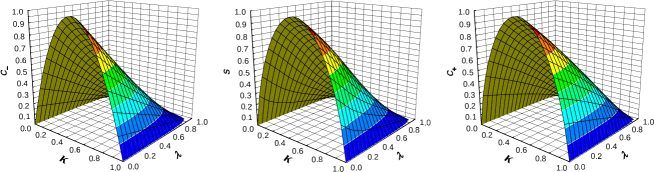
Figure 1: The coefficients $C_{-}$ of (2.25) (left panel), $s_{\kappa\lambda}$ of (2.30) – (2.31) (central panel), and $C_{+}$ of (2.25) (right panel) as functions of parameters $\kappa$ of (2.17) and $\lambda$ of (1.22).

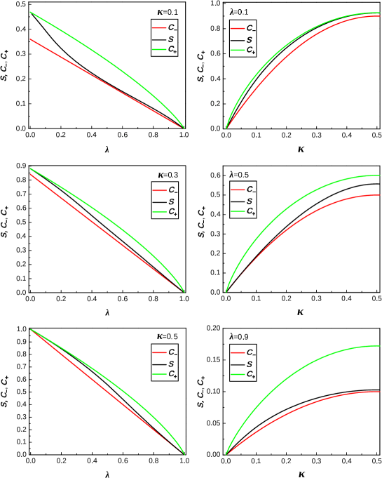
Figure 2: Left: The coefficients $C_{-}$ (red) and $C_{+}$ (green) of (2.25), and $s_{\kappa\lambda}$ (black) of (2.30) as functions $\lambda$ for different values of $\kappa$. Right: The same coefficients as functions of $\kappa$ for different values of $\lambda$.

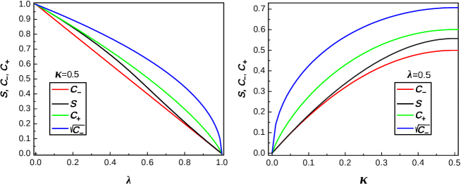
Figure 3: The same as on Fig. 2 and the coefficient $\sqrt{C_{-}}$ (blue) of (2.32).

$\kappa$	$\Delta(C_{-},s)$	$\Delta(s,C_{+})$	$\Delta(C_{-},C_{+})$
0.1	0.10	0.09	0.1
0.2	0.08	0.096	0.1
0.3	0.05	0.08	0.1
0.4	0.05	0.08	0.1
0.5	0.06	0.09	0.1
0.6	0.06	0.08	0.1
0.7	0.05	0.08	0.1
0.8	0.08	0.09	0.1
0.9	0.1	0.09	0.1

$\lambda$	$\Delta(C_{-},s)$	$\Delta(s,C_{+})$	$\Delta(C_{-},C_{+})$
0.1	0.07	0.04	0.1
0.2	0.06	0.07	0.1
0.3	0.06	0.09	0.1
0.4	0.06	0.09	0.1
0.5	0.06	0.09	0.1
0.6	0.04	0.09	0.1
0.7	0.02	0.08	0.1
0.8	0.014	0.09	0.1
0.9	0.01	0.07	0.07

Table 1: Maximal distances between the coefficients $C_{\pm}$ of (2.25) and $s_{\kappa\lambda}$ of (2.30). Left: $\Delta(C_{-},s)=\max_{\lambda}[s-C_{-}]$, $\Delta(s,C_{+})=\max_{\lambda}[C_{+}-s]$, and $\Delta(C_{-},C_{+})=\max_{\lambda}[C_{+}-C_{-}]$ at different values of $\kappa$. Right: the same distances but with $\max_{\kappa}$ for different values of $\lambda$.

2.3 Entanglement Entropy of Hawking Radiation

The problem is as follows. Viewing black hole and its radiation as a bipartite quantum system (1.1) – (1.2), denote

$$\dim\mathcal{H}_{\mathfrak{B}}=\mathsf{L},\;\dim\mathcal{H}_{\mathfrak{E}}=\mathsf{K},\;\dim\mathcal{H}_{\mathfrak{S}}=\mathsf{KL}=\mathsf{N}.$$ (2.35)

and index the bases in the state spaces $\mathcal{H}_{\mathfrak{B}}$ and $\mathcal{H}_{\mathfrak{E}}$ of its parties by $l=1,\dots,\mathsf{L}$ and $k=1,\dots,\mathsf{K}$.

Note that in the discussed above case of free fermions, where the description reduces to the one-body picture, the indexing sets of the block and its environment are $\Lambda$ and $\Omega\setminus\Lambda$, but in that case $|\Omega|=|\Lambda|+|\Omega\setminus\Lambda|$, while in (2.35) we have $\mathsf{N=KL}$. This is because the second quantization is a kind of the "exponentiation" of the one-body picture.

Assuming the complete ignorance of the structure of the whole system $\mathfrak{S}$ (an evaporating black hole and its radiation), one can choose as its ground state

$$|\Psi_{\mathfrak{S}}\rangle=\{\Psi_{kl}\}_{k,l=1}^{\mathsf{K,L}}$$ (2.36)

the random vector uniformly distributed over the unit sphere in $\mathcal{H}_{\mathfrak{S}}=\mathcal{H}_{\mathfrak{B}}\otimes\mathcal{H}_{\mathfrak{E}}\mathbb{=C}^{\mathsf{N}},$ $\mathsf{N=KL}$ (see (1.2) and (2.35)). Thus, the density matrix $\rho_{\mathsf{N}}$ of $\mathfrak{S}$ and the reduced density matrix $\rho_{\mathsf{LN}}$ of $\mathfrak{B}$ (the radiation) are

$$(\rho_{\mathsf{N}})_{k_{1}l_{1},k_{2}l_{2}}=\Psi_{k_{1}l_{1}}\overline{\Psi_{k_{2}l_{2}}},\;\;(\rho_{\mathsf{LN}})_{l_{1}l_{2}}=\sum_{k=1}^{\mathsf{K}}\Psi_{kl_{1}}\overline{\Psi_{kl_{2}}},$$ (2.37)

(cf. (1.3) – (1.4)).

It is of interest to find the typical behavior of the corresponding (random) entanglement entropy (see (1.5). It was suggested in [33], as a first step in this program, that

$$\mathbf{E}\{S_{\mathsf{LN}}\}=\sum_{t=\mathsf{K}+1}^{\mathsf{KL}}\frac{1}{t}-\frac{\mathsf{L}-1}{2\mathsf{K}},\;\mathsf{L}\leq\mathsf{K}=\mathsf{N/L}.$$ (2.38)

Formula (2.38) was then proved by using an explicit and rather involved form of the joint eigenvalue distribution of random matrix $\rho_{\mathsf{LN}}$ (2.37), see e.g. [6, 27] for reviews.

It follows from (2.38) that the two term asymptotic formula for large $\mathsf{K}$ and any $\mathsf{L}$, i.e., for

$$1\lesssim\ \mathsf{L}\ll\ \mathsf{K}\ \lesssim\mathsf{N}$$ (2.39)

(cf. (1.6)), is

$$\mathbf{E}\{S_{\mathsf{LN}}\}=\log\mathsf{L}-\frac{\mathsf{L}}{2\mathsf{K}}+O(1/\mathsf{K}),\;\mathsf{K}=\mathsf{N/L}\rightarrow\infty.$$ (2.40)

Note that here we follow [33] and use the (cf. (1.6)) standard natural $\log:=\ln$ to the base $e=$2.7182 instead $\log_{2}$ as in the definition (1.5) of the von Neumann entropy.

It follows from (2.38) that in the asymptotic regime of the successive limits (first $\mathsf{K}\rightarrow\infty$, then $\mathsf{L}\rightarrow\infty$ (cf. (1.8) and (2.39)), we have

$$\lim_{\mathsf{K}\rightarrow\infty}\mathbf{E}\{S_{\mathsf{LN}}\}:=\mathbf{E}\{S_{\mathsf{L}}\}=\log\mathsf{L}+o(1),\ \mathsf{L}\rightarrow\infty.$$ (2.41)

Moreover, the same holds in the asymptotic regime of the simultaneous limits $\mathsf{K}\rightarrow\infty$, $\mathsf{L}\rightarrow\infty$, provided that $\mathsf{L}/\mathsf{K}=o(1)$, i.e., $0\leq\alpha<1$ (cf. (1.21)).

This case can be viewed as that describing the very initial stage of the black hole radiation. On the other hand, in the asymptotic regime (cf. (1.21) and (2.28))

$$\mathsf{K}\rightarrow\infty,\;\mathsf{L}\rightarrow\infty,\;\mathsf{L}/\mathsf{K}\rightarrow\lambda>0,$$ (2.42)

another possible implementation of the analog of the heuristic inequalities (1.6) (cf. (1.21) with $\alpha=1$), we have (cf. (1.7))

$$\mathbf{E}\{S_{\mathsf{LN}}\}=\log\mathsf{L}-\left\{\begin{array}[]{cc}\lambda/2,&0\leq\lambda\leq 1,\\ 1/2\lambda+\log\lambda,&\lambda\geq 1.\end{array}\right.$$ (2.43)

This case corresponds to a later stage of the black hole radiation.

It can also be shown that the fluctuations of $S_{\mathsf{LN}}$ vanish for large $\mathsf{K}$ and $\mathsf{L}$, see e.g. [6].

Basing on the formula (2.43), an interesting scenario of the black hole evaporation was proposed in [9, 33], see also [2] for a recent review.

Here we only mention that function given by the r.h.s. of (2.43) (see Figure 4) is monotone increasing, convex and piece-wise analytic. Its $p$th derivative has a jump from $0$ to $(-1)^{p}(p-1)!(p/2-1)$ for all $\;p\geq 3$, "a phase transition" of the third order takes place.

Recall that the maximum of the von Neumann entropy (1.5) over the set of $T\times T$ positive definite matrices of trace 1 is equal to $\log_{2}T$ . We conclude, following [33], that while the (random) states (2.36) (see also (2.48)) of the whole system are pure, the subsystem states are typically quite close to the maximally mixed states with the "deficit" given by the second term of the r.h.s. of (2.43).

The link of the above results with those of the previous subsection is as follows. It was mentioned there that in the case of free fermions the dimension $\dim\mathcal{H}_{\mathfrak{S}}$ of the state space of the system $\mathfrak{S}$ and the volume $|\Omega|=|N|^{d}$ of the domain occupied by $\mathfrak{S}$ are related as $|\Omega|=|N|^{d}=\log_{2}\dim\mathcal{H}_{\mathfrak{S}}$ and the same for its party $\mathfrak{B}$ occupying a subdomain $\Lambda:L^{d}=|\Lambda|=\log_{2}\dim\mathcal{H}_{\mathfrak{B}}$. In fact, this logarithmic dependence is general for the many-body quantum systems. Thus, viewing the black hole and its radiation as the parties of a many-body bipartite system (see (1.1)) and taking into account (2.35), we can interpret $\log L$ in the asymptotic formulas (2.41) – (2.43) as the "volume" of the spatial domain occupied by the black hole radiation, hence, these asymptotic formulas are the analogs of the volume law (1.11), see (2.22) and (2.29) in particular.

We will show now that the standard facts of random matrix theory, that date back to the 1960s, provide a streamlined proof of the validity of (2.41) – (2.43) for a rather wide class of random vectors including those of (2.36) and not only for the expectation of the entanglement entropy but also for its all typical realization, i.e., with probability 1. One can say that these results manifests the typicality and the universality of Page’s formula, given by the r.h.s. of (2.43) and (2.50). For other versions of these important properties see [6, 27, 42].

Let

$$\{X_{lk}\}_{l,k=1}^{\infty},\;\mathbf{E}\{X_{lk}\}=\mathbf{E}\{X_{lk}^{2}\}=0,\;\mathbf{E}\{|X_{lk}|^{2}\}=\xi^{2}>0$$ (2.44)

be an infinite collection of independent identically distributed (i.i.d.) complex random variables with zero mean and unit variance,

$$X_{\mathsf{L}\mathsf{N}}=\{X_{lk}\}_{l,k=1}^{\mathsf{L},\mathsf{K}}$$ (2.45)

be the $\mathsf{K}\times\mathsf{L}$ matrix and

$$Z_{\mathsf{L}\mathsf{N}}=\mathrm{Tr}X_{\mathsf{L}\mathsf{N}}X_{\mathsf{L}\mathsf{N}}^{\ast}=\sum_{l=1}^{\mathsf{L}}\sum_{k=1}^{\mathsf{K}}|X_{lk}|^{2}.$$ (2.46)

View $X_{\mathsf{L}\mathsf{N}}$ as a random vector in

$$\mathbb{C}^{\mathsf{N}}=\mathbb{C}^{\mathsf{K}}\otimes\mathbb{C}^{\mathsf{L}},\;\mathsf{N}=\mathsf{KL,}$$ (2.47)

and (2.46) as the square of its Euclidian norm and introduce the corresponding random vector of unit norm (cf. (2.36))

$$\Psi_{\mathsf{N}}=X_{\mathsf{L}\mathsf{N}}/Z_{\mathsf{L}\mathsf{N}}^{1/2}.$$ (2.48)

Note that if $\{X_{kl}\}_{k,l=1}^{\infty}$ are the complex Gaussian random variables with zero mean and unit variance, then $\Psi_{\mathsf{N}}$ of (2.48) is uniformly distributed over the unit sphere of $\mathbb{C}^{\mathsf{N}}$ (see (2.47)), hence, coincides with (2.36) and the setting of [33].

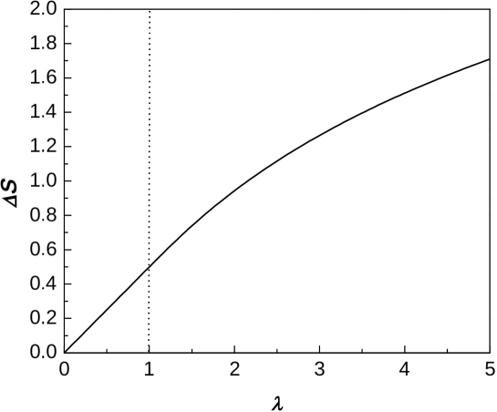
Figure 4: The "deficit" $\Delta=-(S_{\mathsf{LN}}-\log\mathsf{L})$ of (2.43) (and (2.50) and (E.20)) as function of $\lambda$.

Result 2.4

Consider a bipartite quantum systems having the random vector (2.48) as its ground state. Let $S_{\mathsf{LN}}$ be the entanglement entropy defined by (1.5), and (2.37) with $\Psi_{\mathsf{N}}$ of (2.48). Then we have the analogs of (2.41) – (2.43) valid for all typical realizations of (2.48) (with probability 1 with respect to (2.44))

$$\lim_{\mathsf{K}\rightarrow\infty}S_{\mathsf{LN}}:=S_{\mathsf{L}}=\log\mathsf{L}+o(1),\ \mathsf{L}\rightarrow\infty,$$ (2.49)

and

$$S_{\mathsf{LN}}=\log\mathsf{L}-\left\{\begin{array}[]{cc}\lambda/2,&0\leq\lambda\leq 1,\\ 1/2\lambda+\log\lambda,&\lambda\geq 1,\end{array}\right.+o(1),\;\;\mathsf{K,L}\rightarrow\infty,\;\mathsf{L}/\mathsf{K}\rightarrow\lambda>0.$$ (2.50)

One can say that these results manifests the typicality (the validity with probability 1) and the universality (the independence of the probability law of $\{X_{jk}\}$) in (2.44)) of Page’s formula, given by the r.h.s. of (2.43) and (2.50). For other versions of these important properties see [6, 27, 42].

The proof of the result is given in Appendix E.

3 Conclusions

Our main motivation was to study possible asymptotic forms of entanglement entropy of quantum bipartite systems in a regime where the size of one of the parties (block) grows simultaneously with the size of the system. We believe that this regime is of interest both in itself and because it seems more adequate for interpreting numerical results. The regime can be considered for various cases of interaction radii and hopping in the Hamiltonian of the system.

Using a random matrix as a one-body Hamiltonian can serve as a model for long-range hopping whose radius is of the same order of magnitude as the size of the system. We show that in this case the asymptotic behavior of the entanglement entropy follows the volume law, but not the area law or the enhanced area law, that arises in the case of finite-range hopping and the widely used asymptotic regime in which the block size is considered large only after a macroscopic limit passage for the entire system.

For the proof, we use both new seemingly quite general two-sided bounds for the entanglement entropy and existing rigorous results from random matrix theory. The latter also proved to be useful for analyzing the generalization of the Hawking radiation model in the theory of black holes. This analysis, which turns out to be fairly simple and transparent, is also presented in the paper. It implies the validity of the Page formula, obtained initially for a particular case, in quite wide class of typical random states of the system.

4 Acknowledgments

L.P. is grateful to Ecole Normale Superieure (Paris) and l’Institut des Hautes Etudes Scientifiques (Bures-sur-Ivettes) for their kind hospitality during the first stage of the work. Special thanks are due to Prof. E. Brezin for many interesting discussions.

Appendix A Proof of Result 2.1.

The proof is based on the following properties of $h$ and $h_{0}$ of (1.18) and (2.3) which are easy to check, see, e.g. [19]:

(i) $h$ is concave ($h^{\prime\prime}(x)\leq 0,\;x\in(0,1)$) and

$$h(x)\geq 4x(1-x),\;x\in[0,1];$$ (A.1)

(ii) $h_{0}$ of (2.3) is also concave ($h_{0}^{\prime\prime}(y)\leq 0,\;y\in(0,1/4)$) ) and

$$h_{0}(y)=-y\log_{2}y+O(y),\;y\searrow 0.$$ (A.2)

To get the lower bound in (2.1), we denote by $\{p_{\alpha}\}_{\alpha=1}^{|\Lambda|}$ the eigenvalues of $P_{LN}$ of (1.16) and use (A.1) and (2.2):

$$S_{LN}=\operatorname{Tr\,}h(P_{LN})=\sum_{\alpha=1}^{|\Lambda|}h(p_{\alpha})$$

$$\geq\sum_{\alpha=1}^{|\Lambda|}4p_{\alpha}(1-p_{\alpha})=4\operatorname{Tr\,}P_{LN}(\mathbf{1}_{\Lambda}-P_{LN})=:\mathcal{L}_{LN}.$$ (A.3)

To get the upper bound in (2.1), we use (2.2) (or (A.3)), (2.3), and the concavity of $h_{0}$, implying by the Jensen inequality

$$S_{LN}=\sum_{\alpha=1}^{|\Lambda|}h(p_{\alpha})=\sum_{\alpha=1}^{|\Lambda|}h_{0}(p_{\alpha}(1-p_{\alpha}))$$

$$=|\Lambda|\;\Big{(}|\Lambda|^{-1}\sum_{\alpha=1}^{|\Lambda|}h_{0}(p_{\alpha}(1-p_{\alpha})\Big{)}\leq|\Lambda|\;h_{0}\Big{(}(4|\Lambda|)^{-1}\;\mathcal{L}_{\Lambda\Omega})=:\mathcal{U}_{LN}.$$

To get (2.4) – (2.5), we just apply the expectation to (2.1) and use once more the Jensen inequality in the r.h.s.

$$\mathbf{E}\{\mathcal{U}_{LN}\}=|\Lambda|\mathbf{E}\{h_{0}((4|\Lambda)^{-1}|\mathcal{L}_{LN}\}\leq|\Lambda|h_{0}\big{(}(4|\Lambda)^{-1}|\mathbf{E}\{\mathcal{L}_{LN}\}\big{)}.$$

Appendix B Proof of Result 2.2

We will use the bounds (2.1) – (2.3). It follows from (2.16) that the expectation of the lower bound $\mathcal{L}_{LN}$ is expressed via the mixed fourth moments of the entries $\{U_{kl}\}_{k,l=1}^{N}$ of the Haar distributed unitary matrix $U_{N}$. The moments are known (see, e.g. [31], Problem 8.5.2)

$$\mathbf{E}\{U_{a_{1}b_{1}}\overline{U}_{\alpha_{1}\beta_{1}}U_{a_{2}b_{2}}\overline{U}_{\alpha_{2}\beta_{2}}\}$$

$$=(n^{2}-1)^{-1}\big{(}\delta_{a_{1}\alpha_{1}}\delta_{b_{1}\beta_{1}}\delta_{a_{2}\alpha_{2}}\delta_{b_{2}\beta_{2}}+\delta_{a_{1}\alpha_{2}}\delta_{b_{1}\beta_{2}}\delta_{a_{2}\alpha_{1}}\delta_{b_{2}\beta_{1}}\big{)}$$

$$-(n(n^{2}-1))^{-1}\big{(}\delta_{a_{1}\alpha_{2}}\delta_{b_{1}\beta_{1}}\delta_{a_{2}\alpha_{1}}\delta_{b_{2}\beta_{2}}+\delta_{a_{1}\alpha_{1}}\delta_{b_{1}\beta_{2}}\delta_{a_{2}\alpha_{2}}\delta_{b_{2}\beta_{1}}\big{)}$$ (B.1)

and we obtain for $1\leq l<m\leq N$

$$\mathbf{E}\{|P_{lm}|^{2}\}=\sum_{k_{1},k_{2}=1}^{K}\mathbf{E}\{U_{lk_{1}}U_{mk_{2}}\overline{U_{mk_{1}}}\,\overline{U_{lk_{2}}}\}=\frac{1}{(N^{2}-1)}\sum_{k_{1},k_{2}=1}^{K}(\delta_{k_{1}k_{2}}-N^{-1})\frac{K(N-K)}{N(N^{2}-1)}.$$

This and (2.2) imply

$$\mathbf{E}\{\mathcal{L}_{LN}\}=4\sum_{l=1}^{L}\sum_{m=L+1}^{N}\mathbf{E}\{|P_{lm}|^{2}\}=4\frac{K(N-K)L(N-L)}{N(N^{2}-1)},$$ (B.2)

and then (2.1) and (2.17) yield (2.22).

Appendix C Proof of Result 2.3

We will use formulas (2.6) – (2.7) that reduce the problem of the asymptotic analysis of the entanglement entropy to that of the Counting Measure $\mathcal{N}_{P_{{}_{LN}}}$ (2.6) of the random matrix $P_{LN}$ (2.19) in the regime (2.21), more precisely, the limit

$$\nu_{P}=\lim\mathcal{\ N}_{P_{LN}}/L$$ (C.1)

in the sense of (2.21) (see also Appendix E for a similar approach).

The explicit form of $\nu_{P}$ has actually been known since 1980 and is called the Wachter distribution. It was obtained in [43] in the context of statistics, and according to this work, convergence in (C.1) is in probability. In the subsequent works [31, 44, 45, 46] the distribution was obtained by other methods and in other settings, in particular, the convergence with probability 1 was also proved.

We have, according to these works

$$\hskip 42.67912pt\nu_{P}=m_{0}\delta_{0}+m_{1}\delta_{1}+\nu_{ac},$$ (C.2)

$$m_{0} =\max(\lambda-\kappa,0)/\lambda,\;m_{1}=\max(\lambda+\kappa-1,0)/\lambda,$$

and the density $\nu_{ac}^{\prime}$ of $\nu_{ac}$ in (C.2) is given by (2.31). Now, plugging $\nu_{P}$ into the divided by $L$ version of (2.7) for our case, and assuming (2.21), we obtain (2.29) – (2.31), taking into account that the atoms in (C.2) do not contribute to the integral in the r.h.s. of the limiting form of (2.7) because of equalities $h(0)=h(1)=0$.

Note that the atom at 0 in (C.2) can be obtained just by calculating the rank of (2.19) (cf. (E.12)) and the atom at 1 has the same origin, because we have in view of the unitarity of $U_{N}$:

$$(P_{LN})_{l_{1}l_{2}}=\sum_{k=1}^{K}U_{l_{1}k}\overline{U_{kl_{2}}}=\delta_{l_{1}l_{2}}-\sum_{k=K+1}^{N}U_{l_{1}k}\overline{U_{kl_{2}}}.$$ (C.3)

Appendix D Proof of (2.34)

It follows from (1.17), (1.18), and (2.3) that (see also (2.9))

$$S_{LN}=\operatorname{Tr\,}h_{0}(P_{LN}(\mathbf{1}_{\Lambda}-P_{LN})).$$ (D.1)

It is easy to see that if $L=N-1$, then

$$(P_{LN}(\mathbf{1}_{\Lambda}-P_{LN}))_{l_{1}l_{2}}=(P_{\Omega})_{l_{1}N}\overline{(P_{\Omega})_{l_{2}N}},\;l_{1},l_{2}=1,\ldots,(N-1),$$

i.e., it is a hermitian operator of rank one. Hence its eigenvalues are 0 of multiplicity $(L-1)$ and

$$q_{N}=\sum_{l=1}^{N-1}|(P_{\Omega})_{lN}|^{2}$$

of multiplicity 1. This, (2.16), and the unitarity of $U_{N}$ imply

$$q_{N}=u_{N}(1-u_{N}),\;u_{N}=\sum_{l=1}^{N-1}|U_{lN}|^{2},$$ (D.2)

and then, by (D.1)

$$S_{LN}|_{L=N-1}=h_{0}(u_{N}(1-u_{N})),$$

It follows then from the explicit form of the forth mixed moments of the entries $\{U_{lk}\}_{l,k=1}^{N}$ of the Haar distributed matrix $U_{N}$ (see (B.1)) that

$$\hskip 56.9055pt\overline{u}_{N}:=\mathbf{E}\{u_{N}\}=K/N=\kappa(1+O(1/N)),$$

$$\mathbf{Var}\{u_{N}\}:==\mathbf{E}\{|u_{N}-\overline{u}_{N}|^{2}\}\mathbf{=E}\{|u-K/N|^{2}\}\leq\kappa(1-\kappa)N^{-1}(1+O(1/N)),\;N\rightarrow\infty.$$

Hence, by the Tchebychev inequality, we have for any $\varepsilon>0$

$$\mathbf{P}\{|u_{N}-K/N|>\varepsilon\}\leq\mathbf{Var}\{u_{N}\}/\varepsilon^{2}\leq\kappa(1-\kappa)/\varepsilon^{2}N.$$ (D.3)

We conclude by the continuity of $h_{0}$ that for the overwhelming majority of realizations (with probability $1-\varepsilon$ for any $\varepsilon>0$) we have

$$S_{LN}|_{L=N-1}=h_{0}(\kappa(1-\kappa))+o(1),\;\varepsilon\to 0.\;$$ (D.4)

For instance, we can choose $\varepsilon=N^{-1/3}$ to have $O(1/N^{1/3})$ in the r.h.s. of (D.3) and (D.4).

Appendix E Proof of Result 2.4

Following (2.36) – 2.37) and (2.44) – (2.48), we obtain for the corresponding reduced density matrix

$$\rho_{\mathsf{L}\mathsf{N}}=X_{\mathsf{L}\mathsf{N}}X_{\mathsf{L}\mathsf{N}}^{\ast}/Z_{\mathsf{L}\mathsf{N}}.$$ (E.1)

Dividing the numerator and denominator by $\xi^{2}K$, we obtain

$$\rho_{\mathsf{L}\mathsf{N}}=W_{\mathsf{L}\mathsf{N}}/\mathcal{Y}_{\mathsf{L}\mathsf{N}}.$$ (E.2)

where

$$W_{\mathsf{L}\mathsf{N}}=\mathcal{X}_{\mathsf{L}\mathsf{N}}^{\ast}\mathcal{X}_{\mathsf{L}\mathsf{N}}/\mathsf{K},\ \mathcal{Y}_{\mathsf{L}\mathsf{N}}=\mathcal{Z}_{\mathsf{L}\mathsf{N}}/\mathsf{K},\;\mathcal{Z}=\sum_{l,k=1}^{L,K}|\mathcal{X}_{lk}|^{2},$$ (E.3)

and $\{\mathcal{X}_{lk}\}_{l,k=1}^{\infty}$ are independent identically distributed random variables such that (cf. (2.44))

$$\mathbf{E}\{\mathcal{X}_{lk}\}=\mathbf{E}\{\mathcal{X}^{2}_{lk}\}=0,\;\mathbf{E}\{|\mathcal{X}_{lk}|^{2}\}=1.$$ (E.4)

This allows us to write the von Neumann entropy of (E.2) as

$$S_{\mathsf{L}\mathsf{N}}=\log\mathcal{Y}_{\mathsf{L}\mathsf{N}}-\mathcal{Y}_{\mathsf{L}\mathsf{N}}^{-1}\operatorname{Tr\,}W_{\mathsf{L}\mathsf{N}}\log W_{\mathsf{L}\mathsf{N}},$$

$$\hskip 28.45274pt=\log-\mathcal{Y}_{\mathsf{L}\mathsf{N}}--\mathcal{Y}_{\mathsf{L}\mathsf{N}}^{-1}\int w\log w\,\nu_{W_{\mathsf{L}\mathsf{N}}}(dw),$$ (E.5)

where

$$\nu_{W_{\mathsf{L}\mathsf{N}}}=\mathcal{N}_{W_{\mathsf{L}\mathsf{N}}}/\mathsf{L}$$ (E.6)

is the Normalized Counting Measure of eigenvalues of $W_{\mathsf{L}\mathsf{N}}$ (cf. (2.6)).

It follows from the Strong Law of Large Numbers for the collection (2.44) that we have with probability 1 for any $\mathsf{L}$ and $\mathsf{K}\rightarrow\infty$

$$\mathcal{Z}_{\mathsf{L}\mathsf{N}}=\sum_{k,l=1}^{\mathsf{K,L}}|\mathcal{X}_{kl}|^{2}=\mathsf{KL}(1+o(1)),\;\mathsf{N:=KL}\rightarrow\infty.$$ (E.7)

Thus, the first term on the right of (E.5) is in view of (E.3)

$$\log\mathcal{Y}_{\mathsf{L}\mathsf{N}}=\log\mathsf{L}+o(1),\;\mathsf{K}\rightarrow\infty,$$ (E.8)

i.e., it coincides with that in (2.40). Note that this is valid in the both asymptotic regimes, the subsequent limits $\ \mathsf{K}\rightarrow\infty$ and then $\mathsf{L}\rightarrow\infty$ and the simultaneous limits (2.42) and for all typical realizations (with probability 1).

Consider now the second term on the right of (E.5) and assume first that $\mathsf{L}$ is fixed while $\mathsf{K}\rightarrow\infty$. Since (see (E.3))

$$(W_{\mathsf{L}\mathsf{N}})_{l_{1}l_{2}}=K^{-1}\sum_{k=1}^{\mathsf{K}}\mathcal{X}_{l_{1}k}\mathcal{X}_{l_{2}k}^{\ast},\;l_{1},l_{2}=1,\ldots,\mathsf{K},$$ (E.9)

it follows, again from the Strong Law of Large Numbers and (2.44) that $W_{\mathsf{L}\mathsf{N}}$ converges with probability 1 as $\mathsf{K}\rightarrow\infty$ to the $\mathsf{L}\times\mathsf{L}$ unit matrix $\mathbf{1}_{\mathsf{L}}$, thus the second term on the right of (E.5) vanishes as $\mathsf{K}\rightarrow\infty$. We conclude that in the regime of successive limits (see (2.42)) we have with probability 1

$$S_{\mathsf{L}}:=\lim_{\mathsf{K}\rightarrow\infty}S_{\mathsf{L}\mathsf{N}}=\log\mathsf{L},$$ (E.10)

i.e., the version of (2.41) but now for all typical realizations and for not necessarily Gaussian $X_{\mathsf{L}\mathsf{N}}$ of (2.45) with i.i.d. components (2.44). In the context of black hole model of [33, 9] this result corresponds to the maximum mixed state of the Hawking radiation despite the pure initial state (or (2.36) of the whole system (black hole and radiation).

Passing to the regime of the simultaneous limits (2.42), we note first that the matrix $W_{\mathsf{L}\mathsf{N}}$ is known in statistics since the late 1920s as the sample covariance matrix of the sample of $\mathsf{K}$ random $\mathsf{L}$-dimensional vectors $\mathcal{X}_{k}=\{\mathcal{X}_{lk}\}_{l=1}^{\mathsf{L}},\;k=1,\dots,\mathsf{K}$ (data vectors) and according to [47] (see also [31] for a review) the Normalized Counting Measure $\nu_{W_{\mathsf{L}\mathsf{N}}}$ (E.6) of eigenvalues of $W_{\mathsf{L}\mathsf{N}}$ converges with probability 1 to the non random limit (cf. (C.2))

$$\lim_{\mathsf{K\rightarrow\infty,L\rightarrow\infty,L/K}\rightarrow\lambda}\nu_{W_{\mathsf{L}\mathsf{N}}}=:\nu_{W}=\max\{1-\lambda,0\}\delta_{0}+\nu_{ac},$$ (E.11)

$$\nu_{ac}^{\prime}(w)=\frac{\sqrt{(w_{+}-w)(w-w_{-})}}{2\pi\lambda w}\mathbf{1}_{[w_{-},w_{+}]},\;w_{\pm}=(1\pm\sqrt{\lambda})^{2}.$$

Note that the atom at 0 in (E.11) is just (cf. (C.3))

$$\lim_{\mathsf{K\rightarrow\infty,L\rightarrow\infty,L/K}\rightarrow\lambda}(\mathsf{L}-\mathrm{rank}\,W_{\mathsf{LN}})/\mathsf{L}.$$ (E.12)

It follows from (E.6) – (E.8), and (E.11) that the simultaneous limit (2.42) of the second term in (E.5) is

$$I=\frac{1}{2\pi\lambda}\int_{w_{-}}^{w_{+}}\sqrt{(w-w_{+})(w-w_{-})}\,\log wdw.$$ (E.13)

We will use the identity

$$\log w=\int_{0}^{\infty}\left(\frac{1}{t+1}-\frac{1}{t+w}\right)dt,$$

implying

$$I=\lim_{A\rightarrow\infty}(I_{1}-I_{2}),$$ (E.14)

where

$$I_{1} = \frac{1}{2\pi\lambda}\int_{0}^{A}\frac{dt}{t+1}\int_{w_{-}}^{w_{+}}\sqrt{(w-w_{+})(w-w_{-})}dw,\;$$

$$I_{2} = \frac{1}{2\pi\lambda}\int_{0}^{A}dt\int_{w_{-}}^{w_{+}}\frac{\sqrt{(w-w_{+})(w-w_{-})}}{t+w}dw.$$ (E.15)

Changing variables in the integral over $w$ in $I_{1}$ to

$$w=m+lx,\;m=\frac{w_{+}+w_{-}}{2}=(1+\lambda),\;\frac{w_{+}-w_{-}}{2}=2\sqrt{\lambda},$$ (E.16)

we obtain

$$I_{1}=\frac{2}{\pi}\int_{0}^{A}\frac{dt}{t+1}\int_{-1}^{1}\sqrt{1-x^{2}}dx=\int_{0}^{A}\frac{dt}{t+1}=\log A+O(1),\;A\rightarrow\infty.$$ (E.17)

The same change of variables (E.16) yields

$$I_{2}=\frac{l}{2\pi\lambda}\int_{0}^{A}dt\int_{-1}^{1}\frac{\sqrt{1-x^{2}}}{x+\tau}dx,\;\tau=\frac{t+m}{l}>1.$$

The integral over $x$ is $\pi(\tau-(\tau^{2}-1))$, hence, by (E.16)

$$I_{2} = 2\int_{m/l}^{(A+m)/l}\left(\tau-(\tau^{2}-1)^{1/2}\right)d\tau$$ (E.18)

$$= \left.\left(\frac{1}{2}\log(\tau+(\tau^{2}-1)^{1/2})-\frac{1}{4}(\tau-(\tau^{2}-1)^{1/2})^{2}\right)\right|_{\tau=m/l}^{(A+m)/l},$$

Now, taking into account (E.16),

$$\left.\left(\tau+(\tau^{2}-1)^{1/2}\right)\right|_{\tau=m/l} = 2l^{-1}\max(1,\lambda),\;\left.\left(\tau-(\tau^{2}-1)^{1/2}\right)\right|_{\tau=m/l}=$$

$$=2l^{-1}\min(1,\lambda),$$

$$\left.\left(\tau+(\tau^{2}-1)^{1/2}\right)\right|_{\tau=(A+m)/l} = 2Al^{-1}+O(1/A),\;A\rightarrow\infty,$$ (E.19)

and (E.14) – (E.19), we get for $I$ of (E.13)

$$I=2^{-1}\min(\lambda,\lambda^{-1})+\log\;\max(1,\lambda).$$ (E.20)

This coincides with the second term of the r.h.s. of (2.43), hence proves with probability 1 Result 2.4.

References

• [1] Abanin, D. A.; Altman, E.; Bloch, I.; Serbyn, M. Many-body localization, thermalization, and entanglement. Rev. Mod. Phys. 2019, 91, 021001.
• [2] Almheiri, A.; Hartman, T.; Maldacena, J.; Shaghoulian, E.; Tajdini, A. The entropy of Hawking radiation.Rev. Mod. Phys. 2021 93, 35002.
• [3] Amico, L; Fazio, R.; Osterloh, A.; Vedral, V. Entanglement in many body systems. Rev. Mod. Phys. 2008 80, 517–578.
• [4] Aolita, L.; Melo, F.D.; Davidovich, L. Open-system dynamics of entanglement: a key issues review. Rep. Prog. Phys. 2015 78, 042001.
• [5] Calabrese, P.; Cardy, J.; Doyon, B. Entanglement entropy in extended systems. J. Phys. A: Math. Theor. 2009 42, 500301.
• [6] Dahlsten, O.C.O.; Lupo, C.; Mancini, S.; Serafini, A. Entanglement typicality. J. Phys. A: Math. Theor. 2014 47, 363001.
• [7] Deutsch, J. M. Eigenstate thermalization hypothesis. Rep. Prog. Phys. 2018 81, 082001.
• [8] Horodecki, R.; Horodecki, P.; Horodecki, M.; Horodecki, K. Quantum entanglement. Rev. Mod. Phys. 2009 81, 865–942.
• [9] Page, D. N. Hawking radiation and black hole thermodynamics. New Journal of Physics 2005 7, 203.
• [10] Refael, G.; Moore, J. E. Criticality and entanglement in random quantum systems. J. Phys. A: Math. Theor. 2009 42, 504010.
• [11] Szalay, S.; Zimboras, Z.; Mate, M.; Barcza, G.; Schilling, C.; Legeza, O. Fermionic systems for quantum information people. Phys. A: Math. Theor. 2021 54, 393001.
• [12] Witten, E. Notes on some entanglement properties of quantum field theory. Rev. Mod. Phys. 2018 90, 045003.
• [13] Eisert, J.; Cramer, M.; Plenio, M.B. Area laws for the entanglement entropy. Rev. Mod. Phys. 2010 82, 277.
• [14] Laflorencie, N. Quantum entanglement in condensed matter systems. Physics Reports 2016 646, 1–59.
• [15] Peschel, I.; Eisler, V. Reduced density matrices and entanglement entropy in free lattice models. J. Phys. A: Math. Theor. 2009 42, 504003.
• [16] Benatti, F.; Floreanini, R.; Franchini, F.; Marzolino, U. Entanglement in indistinguishable particle systems. Phys. Rep. 2020 878, 1–27.
• [17] Abdul-Rahman, H.; Stolz, G. A uniform area law for the entanglement of the states in the disordered XY chain. J. Math. Phys. 2015, 56, 121901.
• [18] Burmistrova, I.S.; Tikhonova, K.S.; Gornyi, I.V.; Mirlin, A.D. Entanglement entropy and particle number cumulants of disordered fermions. Annals of Physics 2017 383, 140 - 156.
• [19] Elgart A.; Pastur, L.; Shcherbina, M. Large block properties of the entanglement entropy of free disordered fermions. J. Stat. Phys. 2017 166, 1092–1127.
• [20] Leschke, H.; Sobolev, A.; Spitzer, W. Trace formulas for Wiener–Hopf operators with applications to entropies of free fermionic equilibrium states. J. Funct. Anal. 2017 273, 1049–1094.
• [21] Lydzba, P.; Rigol, M.; Vidmar, L. Eigenstate entanglement entropy in random quadratic hamiltonians. it Phys. Rev. Lett. 2020 125, 180604
• [22] Pastur, L.; Slavin, V. The absence of the selfaveraging property of the entanglement entropy of disordered free fermions in one dimension. J. Stat. Phys. 2018 170, 207–220.
• [23] Peschel, I. Calculation of reduced density matrices from correlation functions. J. Phys. A: Math. Gen. 2003 36, L205.
• [24] Pastur, L.; Shcherbina, M. SzegΓΆ-type theorems for one-dimensional Schrodinger operator with random potential. J. Math. Phys., Analysis, Geometry 2018 14, 362 – 388.
• [25] Kirsch, W.; Pastur, L. On the analogues of Szegâ’s theorem for ergodic operators. Sbornik: Mathematics. 2015 206, 93–119.
• [26] Bottcher, A.; Silbermann, B. Introduction to Large Toeplitz Matrices: Springer, Berlin, 1998.
• [27] Bianchi, E.; Hackl, L.; Kieburg, M.; Rigol, M.; Vidmar, L. Volume-law entanglement entropy of typical pure quantum states. Phys. Rev X Quantum 2022 3, 030201.
• [28] Muller, P.; Pastur, L.; Schulte, R. How much delocalisation is needed for an enhanced area law of the entanglement entropy? Comm. Math. Phys. 2020 376, 649–676.
• [29] Lifshitz, I.M.; Gredeskul, S.A.; Pastur, L.A. Introduction to the Theory of Disordered Systems: Wiley, 1989.
• [30] Pastur, L.; Slavin, V. On the universality of the enhanced area law for the entanglement entropy of free fermions, (in preparation).
• [31] Pastur, L.; Shcherbina, M. Eigenvalue Distribution of Large Random Matrices: AMS, Providemce (2011).
• [32] ErdΓΆs, L. Universality of Wigner random matrices: a survey of recent results. Russian Math. Surveys, 2011 66, 507–626 (2011).
• [33] Page, D.N. Average entropy of a subsystem. Phys. Rev. Lett. 1993 71, 1291–1294.
• [34] Page, D. N. Information in black hole radiation. Phys. Rev. Lett. 1993, 71, 3743–3746.
• [35] Kirsch, W.; Lenoble, O.; Pastur, L. On the Mott formula for the ac condactivity and binary correlators in the strong localization regime of disordered systems. J. Phys. A: Math. Gen. 2003 36, 12157–12180.
• [36] Helling, R.; Leschke, H.; Spitzer, W. A special case of a conjecture by Widom with implications to fermionic entanglement entropy. International Mathematics Research Notices 2011 (7)1451–1482.
• [37] Pastur, L.; Slavin, V. Area law scaling for the entropy of disordered quasifree fermions. Phys. Rev. Lett. 2014 113, 150404.
• [38] Wolf, M.M. Violation of the entropic area law for fermions. Phys. Rev. Let. 2008, 96, 010404.
• [39] Landau, H. J.; Widom, H. Eigenvalue distribution of time and frequency limiting. Journal of Mathematical Analysis and Applications 1980 77, 469–481.
• [40] Brezin, E.; Wadia, S. Large $N$ Expansion in Quantum Field Theory and Statistical Physics, The: From Spin Systems to 2-Dimensional Gravity: World Sci. Publ. Singapore, 1993.
• [41] Mezard, M.; Parisi, G.; Virasoro, M.A. Spin Glass Theory And Beyond: World Sciences, Singapore, 1986.
• [42] Nakagawa, Yu. O;, Watanabe, M.; Fujita, H.; Sugiura S. Universality in volume-law entanglement of scrambled pure quantum states. Nat. Comm. 2018 9, 1635.
• [43] Wachter, K. W. The limiting empirical measure of multiple discriminant ratios. The Annals of Statistics 1980 8, 7–957.
• [44] Mingo, J.A.; Speicher, R. Free Probability and Random Matrices: Springer, Berlin, 2017.
• [45] Pastur, L. The law of addition of random matrices revisited. J. Math. Phys., Analysis, Geometry 2023 19, 191–210.
• [46] Vasilchuk, V. On the law of multiplication of random matrices. Mathematical Physics, Analysis and Geometry 2001 4, 1–36.
• [47] Marchenko, V.; Pastur, L. The eigenvalue distribution in some ensembles of random matrices. Math. USSR Sbornik 1967 1, 457–483.