Revisiting model at unphysical pion masses and high temperatures. II. The vacuum structure and thermal pole trajectory with cross-channel improvements
Abstract
The effective potential of model at large limit is reinvestigated for varying pion mass and temperature. For large pion masses and high temperatures, we find the phenomenologically favored vacuum, located on the upper branch of the double-branched effective potential for physical , moves to the lower branch and becomes no longer a local minimum but a saddle point. The existence and running of the tachyon pole are also discussed. With the effective coupling constant defined from the effective potential, the possible correspondence relation between the two branches of the effective potential and the two phases of the theory (distinguished by positive or negative coupling) is verified even with nonzero explicit symmetry breaking and at finite temperature. Also, we generalize the modified model to study the thermal trajectory of the pole with the cross-channel contributions considered and find the thermal pole trajectory resembles its counterpart with varying pion mass at zero temperature.
I Introduction
The well-known linear sigma model [1] is one of the most studied models in quantum field theory. With the help of large expansion, the model becomes exactly solvable at the leading order and demonstrates a variety of non-perturbative properties [2, 3, 4]. When considered as a toy model for low energy pion-pion scattering, this model adopts a linear realization of the chiral symmetry , with the three pseudo-Goldstone bosons, i.e., ’s, combined with another scalar-isoscalar particle . Although this is quite different from the famous chiral perturbation theory [5, 6], where the whole theory lives in the broken phase of QCD and is formulated within the nonlinear realization of chiral symmetry [7, 8], model can be readily applied to studying the restoration of this symmetry at high temperature [9, 10, 11, 12, 13, 14, 15, 16].
With the leading order thermal amplitude obtained in model, our previous work in Ref. [17] showed the detailed pole trajectory and the asymptotic degeneration of and ’s at high temperature, regardless of the different zero-temperature values. And it was also found that at qualitative level, model can describe the behaviors of the lowest pole (dubbed as by PDG [18]) in the channel even for unphysical pion masses. In fact, those behaviors and pole structure have been greatly revealed by analyses on the phase shifts extracted from the lattice QCD data (see, e.g., Refs. [19, 20, 21, 22, 23, 24]).
For a long time, without any explicit symmetry breaking term in the Lagrangian, several interesting features and problems of model have been pointed out and studied in different ways [4, 25, 26, 27, 28, 29, 30, 31]: (a) the two-branch structure of the effective potential and vacuum instability, (b) the existence of a tachyon for the first branch, and (c) the Landau pole and triviality. At large limit, the effective potential of model, , is double-valued hence having two branches [26, 27], which results directly from the non-perturbative effects incorporated by the large expansion. For the first branch, the -component scalar field can acquire a nonzero vacuum expectation value (VEV), whereas for the second, the scalar field’s VEV is always zero [27]. Either branch of has an imaginary part in the large region [27], and this phenomenon was claimed to be a sign for the intrinsic vacuum instability of model [28, 29, 30]. Actually a possible way out is that, if adopting a UV cutoff regularization and viewing the model as an effective theory, it has been shown that the effective potential can be real and convex [31]. Moreover, if choosing the vacuum to be on the first branch, it has been found that there is a tachyonic pole in the scattering amplitude at leading order large expansion, which results from the fact that the local minimum on second branch has lower energy than the one on the first branch [26, 27]. In general, the existence of tachyon could be a severe problem. In fact, the effective potential becomes everywhere complex at next-to-leading order due to the tachyonic pole in the loop integral [25]. But if taking the model as only an effective field theory, the analytically continued matrix can still be considered reasonable in the region far away from the tachyon pole. In this way, the tachyon pole actually labels the “cutoff” scale of model as an effective field theory and thus can be dealt with carefully for higher order calculations [32, 16]. Another problem is related to the divergence of the renormalized coupling constant, i.e., the Landau pole. Unlike the Landau pole found by perturbative calculations of the renormalization group equation (e.g., in QED), which can be ignored in some way since the perturbation series are not suitable anymore when the coupling constant gets large. Unfortunately, the expansion has no similar escape, hence the existence of Landau pole might be thought as leading to the triviality of model [29]. Though the triviality of four-dimensional scalar field theory is widely acknowledged (see for example, Refs. [33, 34, 35, 36, 37, 38, 39, 40]). Recently, a different point of view proposed in Ref. [41] argues that model is nontrivial at large limit. If the “negative coupling phase” of the theory is acceptable, then model can be nontrivial in the IR region even when the UV cutoff is sent to infinity.
This paper is devoted to revisiting the above problems when symmetry is explicitly broken, especially for unphysical pion masses and at finite temperature. Since those problems already arise at the leading order of large expansion, it is reasonable to explore first the cases with nonzero and temperature at the same order. We hope this may shed more light on the understanding of the non-perturbative region of a quantum field theory like model. Additionally, the pole trajectory with varying temperature is obtained in the modified model for completeness of the calculation in Ref. [17], where the pole trajectory is determined only by the leading order thermal amplitude.
The outline is as follows. In Sec. II, the model effective potential at zero temperature is quickly reviewed. We carefully investigate the vacuum structure with varying and obtain a criterion for the existence of tachyon. In Sec. III, the finte-temperature effective potential is studied with different values and the running of tachyon pole is discussed. In Sec. IV, the effective coupling constant is calculated from the effective potential at zero and finite temperature. We verify that the possible correspondence relation between the double-branch structure of the effective potential and the two phases (positive and negative coupling) of model still holds, even with nonzero pion mass and finite temperature. In Sec. V, the modified model is generalized for application at finite temperature and the pole thermal trajectory is obtained with consideration of the cross-channel contributions. Finally in Sec. VI, we briefly summarize the main results and shortly discuss the further issues that could be explored in the future.
II The vacuum structure of model with varying at zero temperature
The linear model is described by the following Lagrangian,
| (1) |
where is an explicit symmetry breaking term and with , pions get massive. In the broken phase, with the symmetry broken into , there are pseudo-Goldstone bosons which can be assigned to the description of pions for . The redefinition of the scalar fields reads, and . It is well known that model is solvable at large limit and this can be standardly calculated through an auxiliary field trick [4], i.e. by introducing another field to the Lagrangian (with an irrelevant constant omitted),
| (2) |
The effective potential of model at the leading order expansion can be standardly calculated as
| (3) |
where and are now reduced to constant values, , and since the pion mass corrections are at higher orders. For brevity, we adopt the same notation for the classical fields and the original fields in the Lagrangian, which can be understood in the context. As in our previous paper Ref. [17], the renormalization conditions are chosen to be [4, 42]
| (4) | ||||
| (5) |
The effective potential can then be expressed in terms of the renormalized quantities as
| (6) |
where the parameters are chosen as with the intrinsic scale of model and . The vacuum is defined at the minimum of the effective potential, thus the conditions and result in the gap equations:
| (7) | |||
| (8) |
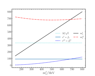
At zero temperature, , according to the partially conserved axial current (PCAC) relation, , where is the axial current, and the definition of the pion decay constant , . Then with Eq. (8), . Actually, the value of is determined by the fact that the zero-temperature gap equations should have a solution at and .
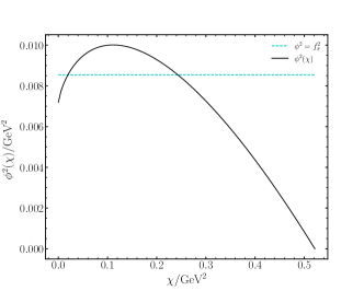
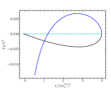
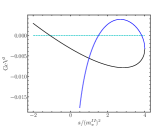
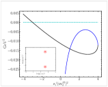
Noting that is in general not identical to the effective potential of the original model defined in Eq. (1). In fact, the model effective potential is recovered after eliminating the auxiliary field by taking as a constraint condition [4, 27]. Thus Eq. (7) will define as function of and the effective potential of model is obtained. However, Eq. (7) has two solutions of which can be easily seen in Fig. 1, where the typical behavior of is shown. The two solutions of are branched at with and thus the effective potential also has two branches and , which is similar to the feature found in model without explicit breaking [26, 27, 28, 29, 30]. From Eq. (7), has a maximum at . It then follows that has a nonzero imaginary part in the region , since in that region there will be no real solutions and has to be complex [4].
Additionally, Eq. (7) shows that for there is another region where it becomes complex. This unphysical region appearing in is very similar to the case that one will encounter in the one-loop perturbative calculation of the effective potential in the broken phase (see textbooks, e.g. Refs. [43, 44]). Fortunately, it should be considered harmless to the theory because the effective potential can still be defined as real and convex when by choosing the state that satisfies to be a proper linear combination of the states corresponding to other field expectation values where is real [44]. However, the above argue does not apply to the former region, i.e. , thus the nonzero imaginary part of along that region and the double-branch feature are actually rooted in the non-perturbative effects captured by the large expansion.
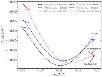
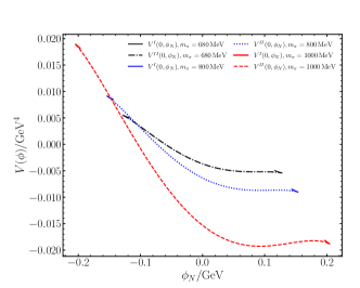
The double-valued effective potentials corresponding to with different ’s are plotted in Fig. 2. For numerical calculations, we always set and MeV. The intrinsic scale of model in leading order calculations is chosen as MeV.
II.1 The local stability of the effective potential
In quantum field theory, the true vacuum state is defined to be at the absolute minimum of the effective potential. The other local minima of correspond to metastable vacuum states (false vacua). Moreover, the local maxima or saddle points are unstable configurations which cannot be viewed as stationary states. Generally, for a convex effective potential, all the vacuum states are among the solutions of gap equations, i. e. Eqs. (7, 8) for model. In Fig. 2, as increases, the local minimum solution with and gradually moves from the first (upper) branch to the second (lower) branch and turns into a saddle point, since and . Then for large pion masses there is no extremum solution on the first branch of the effective potential.
In the following we will show the details about how the vacuum solution becomes a saddle point when it moves to the second branch. Firstly, according to Eq. (7) and Fig. 1, it is straightforward to demonstrate that when seeking for a vacuum at with , the solution lies on ; while with , the solution is on . Besides this solution, there is always another vacuum located on . Expand the effective potential Eq. (6) around the solutions of the gap equations,
| (9) |
where is the shifted field, and , which can be obtained from Eq. (7), is the partial derivative of with respect to at the vacuum solutions . In the above expansion, we have used the relation and Eq. (7), i.e. . Considering that is always satisfied, the criterion for the solution of vacuum to be a local minimum is
| (10) |
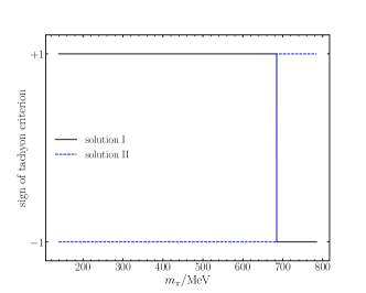
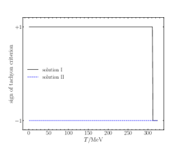
The sign of the criterion for the two solutions (solution I/II, solution I denotes the vacuum at with and solution II is the other vacuum solution to the gap equations at with ) are shown in Fig. 3.
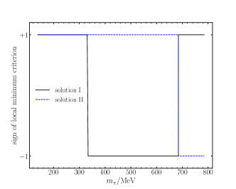
When , both solutions are indeed local minimums as expected. While (with ), the criterion Eq. (10) is unsatisfied, resulting in the solution to be only a saddle point of . For larger pion masses, , the two solutions I and II will hit and move across each other (which can be seen in Fig. 2 and more clearly in Fig. 4), with solution I turns into a local minimum and solution II becomes a saddle point. By definition, the saddle point of the effective potential can not be chosen as the vacuum (or even a false vacuum). In fact, this situation does occur for solution I when (with ) and for solution II when as shown in Fig. 3.
Notably, when using the linear model in the calculation of low-energy pion scattering [17], the phenomenologically favored vacuum is exactly the one on the first branch, , though there is another ”hidden” vacuum state with lower energy on the second branch. 222This may be acceptable since the decay rate of the false vacuum is approximately (see, e.g. Refs. [45, 29]). The phenomena of the local stability of the model effective potential discussed above may imply that for large unphysical , the acceptable vacuum could only be chosen at the second branch and also there should be a sharp transition for the choice of the vacuum state, after the local minimum moves from to and becomes a saddle point.
II.2 The existence of tachyon
It has been complained for a long history that there is a tachyon found in the pion-pion scattering amplitude in model at leading order expansion [4, 27, 42, 32]. Generally, one would argue that the existence of tachyon means the instability of the vacuum. However, things get more complicated in model at large limit, since the effective potential is double-valued and may have two very distinct solutions with respect to the choice of the vacuum. Therefore it should be carefully examined that whether there is still a tachyon pole in each of the gap equation solutions when there is an explicit symmetry breaking term.
In model at leading order, the scattering amplitude [4] is
| (11) |
where is the propagator of the shifted field , such that (for solution I the vacuum expectation value and for solution II, ) [42, 17],
| (12) | ||||
| (13) |
where . The tachyon pole is located at the negative real axis of the -plane with the pole position , which is identified as the zero point of the inverse of Eq. (12) in the region. Thus the existence of tachyon can be analytically determined by a thorough analysis on the zero point distribution of the function along axis. Actually, there is an easy way out: inspired by the analyses of Ref. [27], in the following we will prove that is real and monotonically increasing when . To simplify the discussion, for , let and define , then
| (14) | ||||
| (15) |
It is obvious that as . Furthermore, let and define ,
| (16) | ||||
| (17) |
Since , then with and thus . Considering the definition of the argument , this means that the function is monotonically increasing along the axis. It is trivial that the rest part of , , is also monotonically increasing in that region. Thus the previous argument has been proved. Additionally, when , noting that as , there can only be no more than one zero point, i.e. tachyon pole. The criterion for the existence of tachyon is given by requiring the sign of at to be positive:
| (18) |
which is very similar to the local minimum criterion Eq. (10) and can be verified that they have an identical sign-changing point at (with ), corresponding to the situation when solution I and II meet at the same point. Then there will be a tachyon pole if the criterion Eq. (18) is satisfied and no tachyon pole when the sign of criterion is negative. The result of the examination for the existence of tachyon is shown in Fig. 5. For the local minimum on and the saddle point on , there is always a tachyon, which results from the fact that there exists another vacuum state on with lower energy. However, the existence of tachyon for solution I is not a disaster [42], if we just regard the model as an effective theory of low energy pion dynamics and the validity range of model can be approximately taken to be and for real values, where is the threshold.
II.3 The particle spectrum for the second branch
At zero temperature, the channel particle spectrum for the vacuum solution on the second branch of can be extracted from the partial wave amplitude [4, 42, 17],
| (19) |
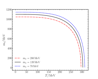
where the and values are set for solution II of the gap equations Eqs. (7, 8), and is defined in Eq. (13). The results distinguished by different pion mass values of solution I () are shown in Fig. 6. When increases from its physical value MeV, the particle spectrum for the second branch of the effective potential demonstrates four different types of contents sequently: (i) two bound states and one virtual state; (ii) one bound state, one virtual state and one tachyon; (iii) two virtual states and one tachyon; (iv) one resonance and one tachyon. Moreover, for not too far from the physical value (e.g., ), the value of is always much larger than that of solution I and hence results in a much smaller value, which can be found out in Fig. 4 and Eq. (7) and Eq. (8). The physics described by solution II is very different compared to the particle spectrum and pole trajectories shown in Ref. [17], where the vacuum is actually always chosen as solution I, originally located on the first branch of the effective potential. Thus in model, for pion masses not too larger than the physical value, the phenomenologically preferred vacuum is on the first branch, not the second branch, as mentioned before.
III The vacuum structure of model with varying at finite temperature
The finite temperature effective potential of model with explicit symmetry breaking at leading order expansion is [12]:
| (20) | ||||
| (21) |
where , and is the Bose-Einstein distribution. The finite temperature contribution can be standardly obtained using the imaginary time formalism [46].
The gap equations are then obtained again by the requirements and ,
| (22) | |||
| (23) |
where and . The function is defined as the finite temperature contribution to the tadpole integral encountered in the derivation of Eq. (7) [17],
| (24) |
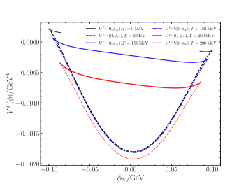
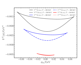
The function defined by Eq. (22) has the same typical behavior as the one at in Fig. 1 (with , and varying with temperature, i.e. , and ). The effective potential at finite temperature (shown in Fig. 7) is obtained by substituting with and solved from Eq. (22) respectively ( ). Though is still double-valued when , it has different behaviors compared to the case with varying in Fig. 2. As temperature increases, and decrease. When the former reaches the point , will be totally real in the region ; while as the latter moves towards zero, and get closer to each other. In the high temperature regime with , where is the critical temperature for chiral restoration in model without explicit symmetry breaking [11, 12], there exists an upper bound for the temperature, namely . Before reaches zero and when temperature gets very high such that , there are no solutions for the gap equations.
III.1 The local stability of the effective potential
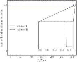
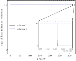
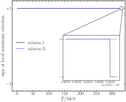
At finite temperature, whether the vacuum solutions of the gap equations are indeed local minima of the effective potential remains to be verified. Due to the finite temperature corrections coming from the loop integrals, the criterion Eq. (10) for the vacuum solution to be a local minimum should be modified as
| (25) |
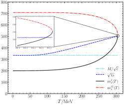
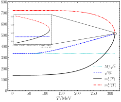
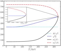
With temperature increasing, both (solution I) and (solution II) are getting closer gradually to each other and finally meet around on the second branch of the effective potential at (see Fig. 8). For , as mentioned before, there are no solutions of the gap equations.
With the criterion Eq. (25), it is found (results shown in Fig. 9) that solution I remains a local minimum when it is on and becomes a saddle point after moving to the second branch as ; whereas solution II is always a local minimum of .
III.2 The existence of tachyon
At finite temperature, the existence of tachyon can be similarly determined by analyzing the zero point distribution of the inverse of the scattering thermal amplitude in model (e.g., for channel, , which has been used in Ref. [17] to trace the pole trajectory with varying temperature). For the consideration of tachyon pole, it would be enough to study the zero point of ,
| (26) |
which is the finite temperature version of and the function is a one-loop two-point integral encountered in model large calculation [17] and standardly it can be decomposed into the zero-temperature part and the finite-temperature part, respectively [46]:
| (27) | ||||
| (28) |
with defined in Eq. (13) and evaluated in the center-of-momentum (CM) frame and . It is obvious that is real and monotonically increasing in the region. Then with a similar argument as the zero-temperature situation, the function is monotonically increasing when and as . Thus the number of zero points of along axis, i.e. tachyons, is no more than one which is the same as the zero temperature case. Similarly, the existence of tachyon at finite temperature is decided by the sign of at . The criterion for tachyon to be present at finite temperature is given below as,
| (29) |
The results of the examination for the existence of tachyon with varying temperature are shown in Fig. 10.
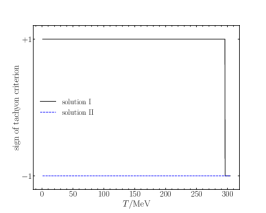

Notably, for large unphysical pion masses and high temperatures the tachyon pole position will move towards the positive real -axis which is shown in Fig. 11. Since the validity range of model can be approximately taken to be and for real . It means that the applicability of model is limited and suppressed as pion mass becoming large and temperature going high.

IV The double-branch effective potential and the two phases of model
The double-valued feature of the model effective potential at large limit has been known for a long time [26, 27, 28, 29, 30, 31]. However, besides the mathematical results, not so much physics has been understood about the nature of the two branches of . For zero temperature and without explicit symmetry breaking, an interesting discovery in Ref. [28] states that the effective coupling constant obtained from the effective potential has opposite signs on the two branches, i.e., the effective coupling constant is positive on the first branch and negative on the second. In the following, we reinvestigate this correspondence for nonzero explicit symmetry breaking and finite temperature.
As usual, the effective coupling constant can be defined as
| (30) |
At zero temperature, the effective coupling can be exactly calculated,
| (31) |
where is solved from Eq. (7) which has two solutions of corresponding to the two branches respectively and is the renormalized coupling constant evaluated at the scale . can be obtained from the -function of model at leading order,
| (32) |
The result is simply expressed as
| (33) |
with the intrinsic scale of model where the coupling constant diverges, i.e. the Landau pole. The sketch of the renormalized coupling constant is shown in Fig. 12.
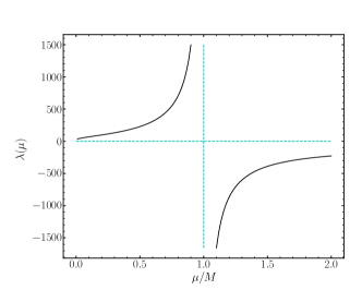
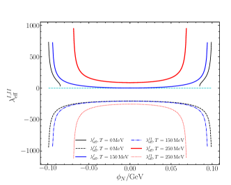
In fact, it can be seen from Eq. (31) that for the first branch and for the second branch. In other words, the two branches of the effective potential still correspond to the two branches of the renormalized coupling constant, with corresponding to the positive coupling branch whereas corresponding to the negative coupling branch. At finite temperature, this relation between the double-branched effective potential and the two phases of model (positive and negative coupling) is also verified (numerically) and shown in Fig. 13. The above results are actually consistent with a recent argument in Ref. [41] that model is not trivial even with infinite UV cutoff, if the negative coupling phase is acceptable. Remarkably, the negative coupling does not make the vacuum unstabler, which has been clearly seen in Refs. [26, 27, 28, 31] when there is no explicit breaking. Instead, the vacuum is stabilized by the non-perturbative effects captured in the large expansion. It has been shown in Sec. II and III that with massive pions for the first branch and at finite temperature, the second branch of effective potential always has a local minimum with lower energy.
V Sigma pole thermal trajectory in modified model
With the method, it has been shown in Ref. [17] that at zero temperature, the crossing symmetry of model in the large limit could be partially recovered while preserving unitarity. In fact, a similar procedure can be also applied to model with finite temperature and can offer a more complete knowledge of the thermal properties of the sigma particle, after taking account of the thermal contribution from crossed-channels.
With respect to the case of model at zero temperature [17], we can add the - and -channel contributions in a similar way and after isospin decomposition and partial wave projection, the channel thermal amplitude is expressed as
| (34) |
where
| (35) | ||||
| (36) | ||||
| (37) |
with and solved from the leading order gap equations Eqs. (22, 23) on the first branch of the effective potential, and defined as Eqs. (27, 28). is the channel partial wave projection integral of the cross-channel thermal amplitude. The definition of appearing in the cross-channel thermal amplitude will be demonstrated as follows. Since at finite temperature, Lorentz invariance is not satisfied anymore, things become more complicated when dealing with the cross-channel thermal loop integral . In fact, the thermal loop integrals rely independently on the temporal and spatial components of the external momentum. As a result, crossing symmetry is also broken and for scattering the contributions from - and -channel are the same [47, 48]:
| (38) | ||||
| (39) |
It is worth mentioning that the calculations of the thermal amplitudes are all conducted in the CM frame.
From the leading order finite temperature amplitude for channel in model, a generalized unitarity relation called “thermal unitarity” [47, 48, 49] can be verified,
| (40) |
with where . While as an approximation, Eq. (34) incorporates the - and -channel contributions which are at , hence breaking the above relation. In pursuit of recovering the thermal unitarity, the method can be adapted accordingly to studying thermal properties of the particle within modified model. The thermal amplitude can be expressed as
| (41) |
with containing only the left-hand cut () and containing only the right-hand cut (), i.e. the thermal unitary cut. In the light of the thermal unitarity relation Eq. (40), we can obtain the relations between and :
| (42) | ||||
| (43) |
It is straightforward to write down dispersion relations for and by using the Cauchy integral. For the same reason, we still use twice subtracted dispersion relations as the zero-temperature case [17] for consistency. The dispersion relations for and can then be written as
| (44) | ||||
| (45) |
where the subtraction points , , and are chosen for convenience. With these choices, the subtraction constants are , , . The is extracted from Eq. (34) as part of the model input. Then the functions and can be solved numerically after setting the subtraction constants.
According to the prescription chosen for the modified model at zero temperature [17], with finite temperature the subtraction constants are determined consistently to be
| (46) | ||||
| (47) | ||||
| (48) |
When ignoring the contributions, the above choice of subtraction constants can exactly recover the leading order thermal amplitude of the model. The main difference between the finite temperature and the zero-temperature prescriptions is that for high temperatures such that becomes a bound state, there is no need to restrict the bound state pole positions in -channel and crossed channels to be the same, due to the breaking of crossing symmetry caused by the thermal loop integrals. In addition, the intrinsic scale is now set with a different value GeV (in consistency with Ref. [17]) due to the higher order contributions incorporated through the unitarization of the model scattering amplitude.
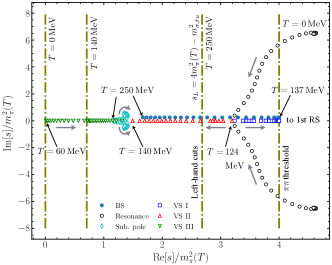
The numerical results of the sigma pole thermal trajectory is depicted in Fig. 14. When temperature increases, similar to the leading order result [17], the broad resonance firstly turns into two virtual states (VS I and II) and then becomes a bound state (BS) after the upper virtual state, VS I, moves towards and through the threshold to the first Riemann sheet. For ( MeV), the bound state pole moves close to , i.e., tends to become asymptotically degenerate with pions, as expected by the chiral symmetry restoration. This behaviour is similar to the leading order calculation in Ref. [17], however the main differences are as follows. With cross-channel thermal contributions, the left-hand cut extends to with where is determined by the bound state pole positions in the - and -channel thermal amplitudes, which are identical for scattering. Additionally, there is a third virtual state (VS III) generated close to . For higher temperatures, VS II and III move towards and then hit each other, becoming a pair of subthreshold poles, which are similar to those also found in Refs. [21, 17] for large unphysical pion mass at zero temperature. Finally, the subthreshold poles move close to as . This results directly from the fact that, on the second Riemann sheet , thus as for high temperatures with the subtraction constants set as Eqs. (47,48).
To one’s surprise, the thermal pole trajectory demonstrates again analogous structure and behavior with the pole trajectory with varying at zero temperature. Actually, this phenomenon is understandable since the third virtual state, VS III, and the subthreshold poles are generated mainly by the interplay of (thermal) unitarity and the cross-channel bound state exchange effects [21, 17].
VI Conclusions and discussions
In this work, we revisit the leading order effective potential of the linear model with explicit symmetry breaking. After careful investigation for the cases of different pion masses and temperatures, a new phenomenon is found for large values and high temperatures. As either or temperature increases, the local minimum on the first branch of the effective potential will move to the second branch and turn into a saddle point. Then the stable vacuum can only be chosen on the second branch. However, the second branch is not preferred for values not so far from the physical value, since it cannot give the right phenomenological results.
On the other hand, at larger and higher temperature, the tachyon pole moves towards the positive real axis, causing the validity domain of model to shrink (when the vacuum is set as the first-branch solution of the gap equations Eqs. (22, 23)). Additionally, with the help of the effective coupling constant, we propose a possible correspondence relation between the double-valued effective potential and the two phases (positive and negative coupling) of model, even with nonzero explicit symmetry breaking and at finite temperature.
As for a thermal generalization of the modified model discussed in our previous work in Ref. [17], the pole trajectory at finite temperature is also obtained with the cross-channel contributions considered. The thermal trajectory resembles its counterpart for varying pion mass at zero temperature.
One of the possible issues for future study could be considering the effects made to the vacuum structure of model at nonzero and finite temperature by including high dimensional terms and higher order contributions. Moreover, the lessons learned in model may arouse interests about the structure of the QCD vacuum at large pion masses and high temperatures.
Acknowledgements.
This work is supported by China National Natural Science Foundation under contract No. 12335002, 12375078, 11975028. This work is also supported by “the Fundamental Research Funds for the Central Universities”.References
- Gell-Mann and Lévy [1960] M. Gell-Mann and M. Lévy, Nuovo Cim. 16, 705 (1960).
- Dolan and Jackiw [1974] L. Dolan and R. Jackiw, Phys. Rev. D 9, 3320 (1974).
- Schnitzer [1974] H. J. Schnitzer, Phys. Rev. D 10, 1800 (1974).
- Coleman et al. [1974] S. R. Coleman, R. Jackiw, and H. D. Politzer, Phys. Rev. D 10, 2491 (1974).
- Gasser and Leutwyler [1984] J. Gasser and H. Leutwyler, Annals Phys. 158, 142 (1984).
- Gasser and Leutwyler [1985] J. Gasser and H. Leutwyler, Nucl. Phys. B 250, 465 (1985).
- Coleman et al. [1969] S. R. Coleman, J. Wess, and B. Zumino, Phys. Rev. 177, 2239 (1969).
- Callan et al. [1969] C. G. Callan, Jr., S. R. Coleman, J. Wess, and B. Zumino, Phys. Rev. 177, 2247 (1969).
- Meyers-Ortmanns et al. [1993] H. Meyers-Ortmanns, H. J. Pirner, and B. J. Schaefer, Phys. Lett. B 311, 213 (1993).
- Meyer-Ortmanns [1996] H. Meyer-Ortmanns, Rev. Mod. Phys. 68, 473 (1996), arXiv:hep-lat/9608098 .
- Bochkarev and Kapusta [1996] A. Bochkarev and J. I. Kapusta, Phys. Rev. D 54, 4066 (1996), arXiv:hep-ph/9602405 .
- Andersen et al. [2004] J. O. Andersen, D. Boer, and H. J. Warringa, Phys. Rev. D 70, 116007 (2004), arXiv:hep-ph/0408033 .
- Amelino-Camelia and Pi [1993] G. Amelino-Camelia and S.-Y. Pi, Phys. Rev. D 47, 2356 (1993), arXiv:hep-ph/9211211 .
- Petropoulos [1999] N. Petropoulos, J. Phys. G 25, 2225 (1999), arXiv:hep-ph/9807331 .
- Lenaghan and Rischke [2000] J. T. Lenaghan and D. H. Rischke, J. Phys. G 26, 431 (2000), arXiv:nucl-th/9901049 .
- Fejos et al. [2009] G. Fejos, A. Patkos, and Z. Szep, Phys. Rev. D 80, 025015 (2009), [Erratum: Phys.Rev.D 90, 039902 (2014)], arXiv:0902.0473 [hep-ph] .
- Lyu et al. [2024] Y.-L. Lyu, Q.-Z. Li, Z. Xiao, and H.-Q. Zheng, Phys. Rev. D 109, 094026 (2024), arXiv:2402.19243 [hep-ph] .
- Workman et al. [2022] R. L. Workman et al. (Particle Data Group), PTEP 2022, 083C01 (2022).
- Briceno et al. [2017] R. A. Briceno, J. J. Dudek, R. G. Edwards, and D. J. Wilson, Phys. Rev. Lett. 118, 022002 (2017), arXiv:1607.05900 [hep-ph] .
- Gao et al. [2022] X.-L. Gao, Z.-H. Guo, Z. Xiao, and Z.-Y. Zhou, Phys. Rev. D 105, 094002 (2022), arXiv:2202.03124 [hep-ph] .
- Cao et al. [2023] X.-H. Cao, Q.-Z. Li, Z.-H. Guo, and H.-Q. Zheng, Phys. Rev. D 108, 034009 (2023), arXiv:2303.02596 [hep-ph] .
- Rodas et al. [2023] A. Rodas, J. J. Dudek, and R. G. Edwards (Hadron Spectrum), Phys. Rev. D 108, 034513 (2023), arXiv:2303.10701 [hep-lat] .
- Rodas et al. [2024] A. Rodas, J. J. Dudek, and R. G. Edwards (Hadron Spectrum), Phys. Rev. D 109, 034513 (2024).
- Rupp [2024] G. Rupp, Phys. Rev. D 109, 054003 (2024), arXiv:2401.08379 [hep-ph] .
- Root [1974] R. G. Root, Phys. Rev. D 10, 3322 (1974).
- Kobayashi and Kugo [1975] M. Kobayashi and T. Kugo, Prog. Theor. Phys. 54, 1537 (1975).
- Abbott et al. [1976] L. F. Abbott, J. S. Kang, and H. J. Schnitzer, Phys. Rev. D 13, 2212 (1976).
- Linde [1977] A. D. Linde, Nucl. Phys. B 125, 369 (1977).
- Bardeen and Moshe [1983] W. A. Bardeen and M. Moshe, Phys. Rev. D 28, 1372 (1983).
- Bardeen and Moshe [1986] W. A. Bardeen and M. Moshe, Phys. Rev. D 34, 1229 (1986).
- Nunes and Schnitzer [1995] J. P. Nunes and H. J. Schnitzer, Int. J. Mod. Phys. A 10, 719 (1995), arXiv:hep-ph/9311319 .
- Ghinculov et al. [1998] A. Ghinculov, T. Binoth, and J. J. van der Bij, Phys. Rev. D 57, 1487 (1998), arXiv:hep-ph/9709211 .
- Aizenman [1981] M. Aizenman, Phys. Rev. Lett. 47, 1 (1981).
- Frohlich [1982] J. Frohlich, Nucl. Phys. B 200, 281 (1982).
- Luscher and Weisz [1987] M. Luscher and P. Weisz, Nucl. Phys. B 290, 25 (1987).
- Luscher and Weisz [1988a] M. Luscher and P. Weisz, Nucl. Phys. B 295, 65 (1988a).
- Luscher and Weisz [1989] M. Luscher and P. Weisz, Nucl. Phys. B 318, 705 (1989).
- Luscher and Weisz [1988b] M. Luscher and P. Weisz, Phys. Lett. B 212, 472 (1988b).
- Hasenfratz et al. [1987] A. Hasenfratz, K. Jansen, C. B. Lang, T. Neuhaus, and H. Yoneyama, Phys. Lett. B 199, 531 (1987).
- Wolff [2009] U. Wolff, Phys. Rev. D 79, 105002 (2009), arXiv:0902.3100 [hep-lat] .
- Romatschke [2023] P. Romatschke, Phys. Lett. B 847, 138270 (2023), arXiv:2305.05678 [hep-th] .
- Chivukula and Golden [1991] R. S. Chivukula and M. Golden, Phys. Lett. B 267, 233 (1991).
- Peskin and Schroeder [1995] M. E. Peskin and D. V. Schroeder, An Introduction to quantum field theory (Addison-Wesley, Reading, USA, 1995).
- Weinberg [2013] S. Weinberg, The quantum theory of fields. Vol. 2: Modern applications (Cambridge University Press, 2013).
- Coleman [1977] S. R. Coleman, Phys. Rev. D 15, 2929 (1977), [Erratum: Phys.Rev.D 16, 1248 (1977)].
- Bellac [2011] M. L. Bellac, Thermal Field Theory, Cambridge Monographs on Mathematical Physics (Cambridge University Press, 2011).
- Dobado et al. [2002] A. Dobado, A. Gomez Nicola, F. J. Llanes-Estrada, and J. R. Pelaez, Phys. Rev. C 66, 055201 (2002), arXiv:hep-ph/0206238 .
- Gomez Nicola et al. [2002] A. Gomez Nicola, F. J. Llanes-Estrada, and J. R. Pelaez, Phys. Lett. B 550, 55 (2002), arXiv:hep-ph/0203134 .
- Gómez Nicola et al. [2023] A. Gómez Nicola, J. R. de Elvira, and A. Vioque-Rodríguez, JHEP 08, 148, arXiv:2304.08786 [hep-ph] .