Different driving protocols and multiple Majorana modes in a Rashba coupled superconducting nanowire

Abstract

We perform systematic analyses of single and multi-frequency driving protocols on a Rashba nanowire with superconducting correlations induced by proximity effects. The results for the single-mode drive reveal interesting frequency dependencies of the Majorana modes, in the sense that the parameters corresponding to the trivial and topological limits of the undriven (static) case host Majorana zero modes, respectively at low and high frequencies. Further, emergence of long-range interactions are noted that give rise to multiple gap-closing scenarios, which imply occurrence of multiple Majorana modes. On the other hand, the multi-frequency driving protocol, sub-grouped into commensurate and incommensurate ratios of the frequencies, demonstrates intriguing consequences. The commensurate case yields dynamical control over the stability of the edge modes. Moreover, complex driving protocols harm the Majoranas by pushing them into the bulk. Finally, the incommensurate case yields independent Majorana modes occurring at low-symmetry points in the Brillouin zone. While the single and the commensurate multi-frequency driving protocols admit the usage of symmetric time frames for the computation of the topological invariants, the incommensurate case relies on the framework of many-mode Floquet theory, where the topological properties are ascertained via calculating the Berry phase. We present band structure and phase diagrams to substantiate all our results. The robustness and concurrent existence of these unique Majorana modes, even amidst a very dense energy spectrum along with a lack of global time-periodicity, hold promise for applications in quantum computing and the development of Floquet time crystals.

I Introduction

Ever since the discovery of integer quantum Hall effect [1], the study of topological states of matter has signaled a pivotal advancement in solid-state research [2, 3, 4, 5, 6]. Exploring and manipulating states that are topologically protected has received substantial interest both theoretically [7, 8, 9] and experimentally [10, 11, 12, 13, 14]. In particular and of relevance to us, topological superconductors (TSCs) have garnered significant attention due to the emergence of exotic quasiparticle excitations akin to Majorana fermions [15]. These Majorana bound states (MBS) associated with TSCs offer a compelling avenue for non-abelian braiding, and conveniently crucial for achieving fault-tolerant quantum computation [16, 17, 18]. The simplest prototype for achieving topological superconductivity was initially proposed by Kitaev, utilizing a one-dimensional model of spinless $p$-wave superconductors [19]. However, the scarcity of $p$-wave superconductors in nature has hindered the experimental realization of Kitaev’s model for TSCs. Nonetheless, the seminal contributions of Fu and Kane [20, 21] have shown that a Kitaev chain can be realized in various systems, utilizing the conventional proximity-induced $s$-wave superconductivity as a key ingredient. Building on their insights, the experimental accessibility of the Kitaev chain has expanded significantly, leading to the proposal of MBS in diverse media such as one-dimensional semiconducting nanowire with Rashba spin orbit coupling (SOC) [22, 23, 24, 25], two-dimensional quantum wells [26, 27], carbon nanotubes [28, 29, 30] and so on.

On a parallel front, the concept of engineering non-trivial states of matter can extend beyond equilibrium conditions. Consequently, Floquet engineering has emerged as an intriguing avenue for the precise tuning of topology in non-equilibrium systems [31, 32, 33]. Furthermore, as a result of the time periodicity, the energy bands can be folded back into a Floquet Brillouin zone (FBZ), at the boundary of which the system facilitates the emergence of anomalous topological states, referred to as $\pi$ modes [34, 35, 36, 37]. This concept has been effectively utilized in numerous experiments involving ultracold atoms in optical lattices out-of-equilibrium conditions and photonic waveguides [38, 39, 40, 41, 42, 43]. Additionally, the time periodicity can be harnessed through the photo-induced band gaps, which further can be resolved by a technique known as time and angle-resolved spectroscopy (t-ARPES) [44, 45]. In recent years, there has been a remarkable surge in interest for studying non-equilibrium topology of systems in the following sense. Is topology robust in a driven scenario? In fact, surprisingly, topology not only survives but gets richer in presence of periodic drive. This encompasses various phenomena, such as the generation of higher winding or Chern numbers in 1D, 2D, and quasi-1D systems [46, 47, 48, 49, 50, 51, 52], emergence of discrete time crystalline phases along with period doubling oscillations [53, 54], topological characterization of quantum chaos models [55, 56], emergence of Floquet-Anderson phases in quasiperiodic systems [57] and so forth.

In the pursuit of understanding non-equilibrium topology, researchers have explored Floquet topological superconductors to reveal dynamical versions of Majoranas, known as Floquet Majorana modes [52, 58, 59, 60, 61, 62]. However, much of this research has been based on Kitaev’s original model involving $p$-wave superconductors. Nevertheless, considering the practicality of experimentation, our attention will pivot towards the Rashba nanowire model, as the exploration of Floquet Majoranas within this model remains relatively uncharted territory, with only a few studies conducted so far [63, 65]. In contrast to the original model, the Rashba nanowire variant incorporates $s$-wave superconducting correlations and a magnetic field that breaks the time-reversal symmetry (TRS). The lack of TRS constrains the number of Majorana modes since the formation of many Majorana modes demands the protection of TRS [58, 64]. This motivates us to look for a scenario whether an external periodic drive (entering through the magnetic field itself) in the present context could admit the emergence of multiple Majorana modes which may have crucial ramifications in topological quantum computation.

Furthermore, in the context of external periodic driving, few fundamental question arises. What are the implications for the generalization of topological properties when the external drive includes more than one frequency? Can we anticipate the coexistence of multiple Majorana modes? If so, then how can we adequately characterize them? In a generic sense, there can be two possible alternatives for multi-frequency driving: (i) when the ratio of the two frequencies is a rational number (commensurate drive), and (ii) when it is an irrational number (incommensurate drive). Recent advancements in Floquet engineering have spurred considerable progress in this area. Specifically, the formalism associated with incommensurate driving expands the dimensionality of the problem by introducing a Fourier manifold corresponding to each frequency [66, 67, 68]. This treatment of creating synthetic dimensions has been extensively explored, yielding practical applications, such as, zero-dimensional qubit mixers [69], energy converters between different drives [66, 70], and stabilizers for dynamic topological phases [71]. However, due to the necessity of additional Fourier dimensions, this approach may pose computational challenges for models exceeding two dimensions. On the contrary, commensurate driving methods, notably two-tone harmonic driving, have found significant application in a range of experimentally achievable settings. These include instances such as quantum destructive interference in the Fermi-Hubbard model [72], sensitivity synchronizer in Rydberg atoms [73], generation of Floquet-Bloch nontrivial band structures [74, 75], etc. Drawing inspiration from these advancements, in this paper along with the single-drive scenario, we seek to examine the topological characteristics of the Rashba nanowire model under a multi-frequency (both commensurate and incommensurate driving) driving protocol.

Our findings are derived from the mapping of the drives into the frequency space, resulting in the emergence of additional Floquet couplings. Consequently, a thorough analysis of frequencies may lead to various instances of non-trivial gap closure, ensuring sustained topological nature of the system even for parameter values that host trivial phases. Furthermore, we aim to utilize the symmetries associated with the stroboscopic time evolution operator, thereby introducing a new approach to the topological classification, where each non-trivial phase is distinguished by the concept of ‘pairs of symmetric time frames’. Furthermore, within a commensurate driving protocol, there exists a possibility to dynamically adjust the stability and the number of Majorana edge modes by carefully tuning the ratio of driving frequencies. Conversely, in presence of an incommensurate driving scenario, the absence of global time periodicity impedes our traditional technique of using an evolution operator and instead demands the usage of the Shirley-Floquet formalism [34, 35, 36, 37]. Unlike the approach of synthetic dimensions demonstrated in Ref. [66], we shall adopt the generalized version of the many-mode Floquet theory illustrated in Ref. [76] and others [77, 78, 79]. This methodology may lead to the emergence of unique Majorana modes that remain stable and can coexist independently with other Majoranas (from the static picture), despite the dense spectra induced by the quasiperiodic nature of the drive.

The layout of the subsequent discussions is as follows: In Sec.II we provide an overview of the static version of the model, revisiting its symmetries and the functionalities of each of the parameters. Following this, we shall introduce the Floquet tool to formulate an effective time-independent Hamiltonian. In Sec.III, we delve into the topological features related to both single-drive and multi-frequency commensurate and incommensurate drives. Finally, in Sec.IV, we provide a summary and draw conclusions based on our findings.

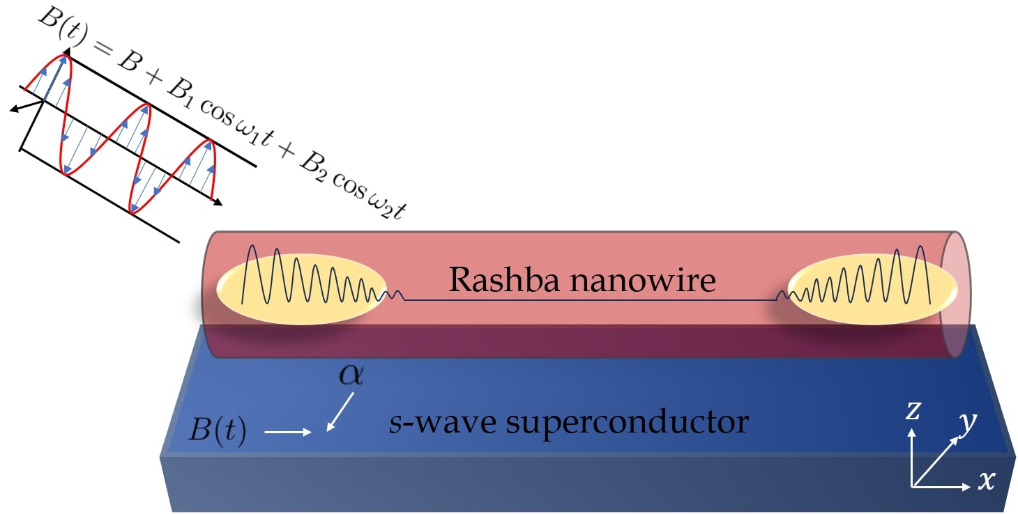
Figure 1: The figure depicts a schematic representation of a Rashba nanowire proximity-coupled to a $s$-wave superconductor subjected to a perpendicular time-modulated magnetic field, $B(t)$.

II The $s$-wave Kitaev chain and the Floquet Formalism

A potential physical realization for engineering topological superconductivity in one dimension based on Kitaev’s model is schematically depicted in Fig. 1. This setup involves the utilization of a semiconductor nanowire, such as InSb, where strong SOC plays a crucial role and is an important ingredient of our study. To provide a visual representation, consider a Kitaev chain in proximity to an $s$-wave pairing which can be denoted as,

$$\mathcal{H}_{SC}=\frac{\Delta}{2}\sum_{i}(c_{i,\uparrow}c_{i,\downarrow}-c_{i,\downarrow}c_{i,\uparrow})+h.c.,$$ (1)

where $\Delta$ represents the superconducting pairing amplitude Moreover, the particle-hole symmetry of the model necessitates the condition $\gamma_{E,\uparrow}^{\dagger}=\gamma_{-E,\downarrow}$ (where $\gamma$ is the Majorana operator). This implies that the existence of a particle being its own antiparticle must occur at zero energy. However, in the case of $s$-wave superconductors, the presence of spin degrees of freedom prevents the existence of robust zero-energy modes. To address this limitation, one may introduce an external magnetic field $B$, such that, if the Hamiltonian for particles is denoted by $H(B)$, then for holes it would be $-H(-B)$. Additionally, considering the presence of spin, there has to be a Zeeman coupling that will change sign under TRS. Another crucial aspect that must be taken into account is that $s$-wave superconductors exhibit singlet pairing, implying that the $z$-component of the total spin is preserved. The Zeeman term also conserves spin in the $z$-direction, and each singlet excitation possesses a definite spin, including the Majoranas. However, this poses a threat to the existence of Majoranas, which should have no definite spin due to their property of being complex conjugate of themselves. Therefore, the only viable solution is to violate spin conservation by introducing a Rashba SOC ($\alpha$), which specifically breaks the $s_{z}$ symmetry. Thus including the Zeeman term, the $s$-wave pairing and the Rashba SOC the Hamiltonian can be written as,

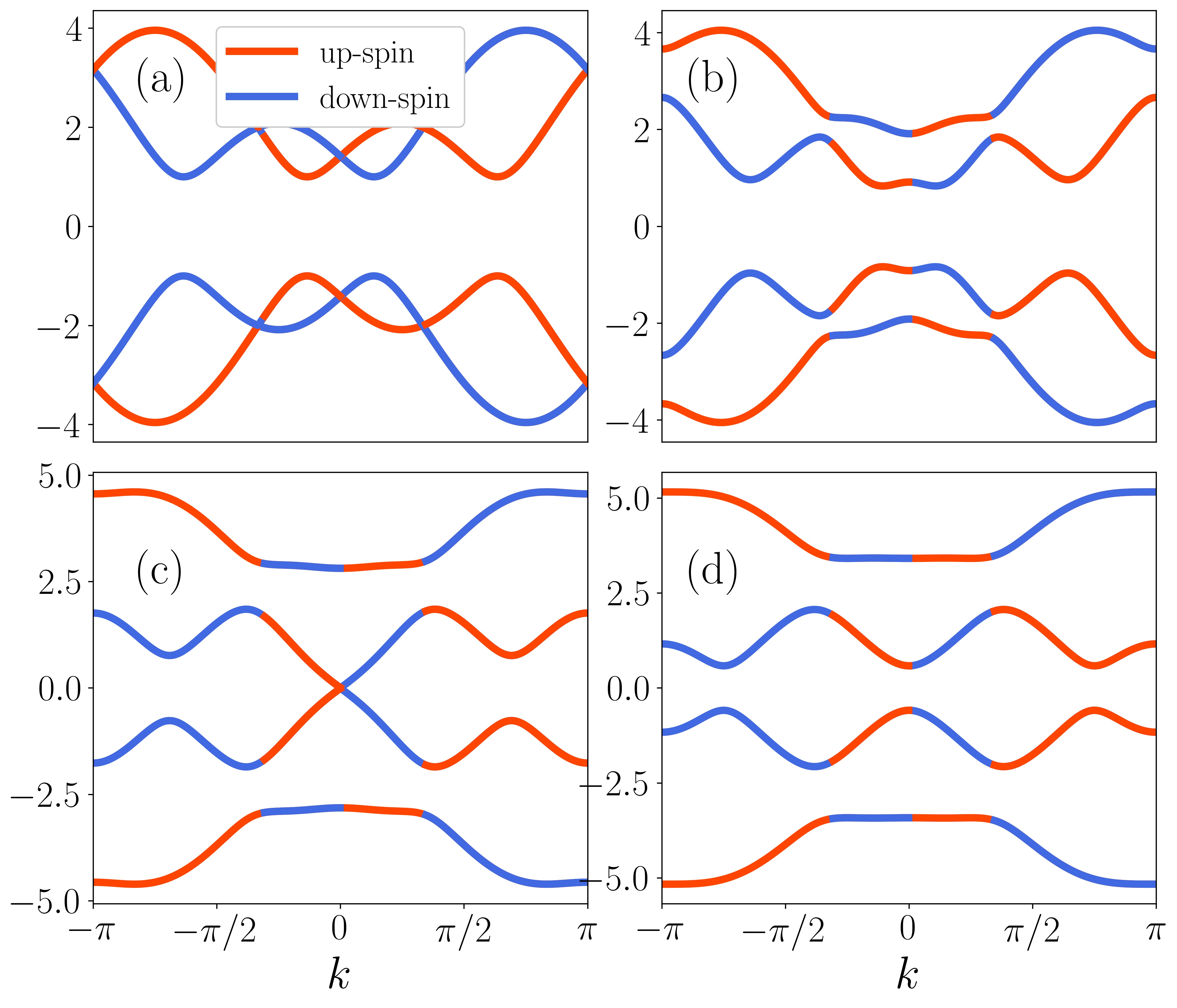
Figure 2: The dispersion spectra corresponding to a static $s$-wave Kitaev chain for different values of the magnetic field, $B$. We study the case of zero field (a), 0.5 $B_{c}$ (b), $B_{c}$ (c), and $1.5B_{c}$ (d). A gap-closing transition (at $k=0$) occurring at $B=B_{c}$ is noted. The other parameter are chosen as, $\mu=0.5,\Delta=0.5,t=1,$ and $\alpha=0.5$.

$$H=\hat{\mathcal{H}}_{kin}+\hat{\mathcal{H}}_{so}+\hat{\mathcal{H}}_{z}+\hat{\mathcal{H}}_{sc}$$ (2)

where,

$$\hat{\mathcal{H}}_{so}=\alpha\sum_{j}\Big{[}\hat{c}^{\dagger}_{j,\downarrow}(\hat{c}_{j+1,\uparrow}-\hat{c}_{j-1,\uparrow})-\hat{c}^{\dagger}_{j,\uparrow}(\hat{c}_{j+1,\downarrow}-\hat{c}_{j-1,\downarrow})\Big{]},$$ (3)

$$\hat{\mathcal{H}}_{z}=\sum_{j}B(\hat{c}^{\dagger}_{j,\uparrow}\hat{c}_{j,\downarrow}+\hat{c}^{\dagger}_{j,\downarrow}\hat{c}_{j,\uparrow})$$ (4)

$$\hat{\mathcal{H}}_{sc}=\frac{1}{2}\sum_{j}\Big{[}\Delta(\hat{c}^{\dagger}_{j,\uparrow}c^{\dagger}_{j,\downarrow}-\hat{c}^{\dagger}_{j,\downarrow}c^{\dagger}_{j,\uparrow})+h.c\Big{]}$$ (5)

and, a usual kinetic energy for the particles in the nanowire given by,

$$\hat{\mathcal{H}}_{kin}=-\mu\sum_{j,\sigma}^{N}\hat{c}^{\dagger}_{j,\sigma}\hat{c}_{j,\sigma}+\sum_{j,\sigma}^{N-1}\Big{[}-t\hat{c}^{\dagger}_{j,\sigma}\hat{c}_{j+1,\sigma}+h.c.\Big{]}$$ (6)

Finally, in the tight binding notations of the Bogoliubov de Gennes (BdG) representation in the Fourier space, the Hamiltonian assumes the form,

$$\begin{split}&H=\sum_{k}\psi^{\dagger}(y)\mathcal{H}(k)\psi(y)dy\\ &\mathcal{H}(k)=[(2t-\mu)-2t\cos{k}]\tau_{z}\sigma_{0}+2\alpha\sin{k}\tau_{z}\sigma_{y}\\ &\qquad~{}~{}~{}~{}+B\tau_{0}\sigma_{x}+\Delta\tau_{y}\sigma_{y}\\ &\psi^{\dagger}=(c^{\dagger}_{k,\uparrow},c^{\dagger}_{k,\downarrow},c_{k,\uparrow},c_{k,\downarrow})\end{split}$$ (7)

Here, $\psi_{k,\uparrow}(\psi_{k,\uparrow}^{\dagger})$ and $\psi_{k,\downarrow}(\psi_{k,\downarrow}^{\dagger})$ represent electron annihilation (creation) operators for the spin up and spin down sectors, and $\sigma,\tau$ denote the spin and particle degrees of freedom, respectively.

At this point, it is crucial to address the symmetries inherent to the model. As previously discussed, the Hamiltonian upholds particle-hole symmetry, with $C=\tau_{x}\sigma_{0}\kappa$ as the particle-hole operator one finds, $C^{-1}\mathcal{H}(k)C=-\mathcal{H}(-k)$. However, it violates time-reversal symmetry, where $T=i\tau_{0}\sigma_{y}\kappa$ yields $T^{-1}\mathcal{H}(k)T\neq\mathcal{H}(-k)$. Consequently, the model is classified under symmetry class D, and characterized by a $\mathbb{Z}_{2}$ invariant that should host at most one pair of Majorana modes [80].

We review the results of the static model in order to set the stage for discussing results corresponding to the driven situation. At $k=0$, the Hamiltonian undergoes a gap-closing transition for a particular value of the magnetic field, namely, $B=B_{c_{1}}=\sqrt{\mu^{2}+\Delta^{2}}$, Further another transition occurs at $k=\pm\pi$ for $B=B_{c_{2}}=\sqrt{(\mu-4t)^{2}+\Delta^{2}}$. These phenomena of bulk gap closing aid in defining the boundaries of the topological phases, as illustrated in Fig. 2, which showcases the spectral

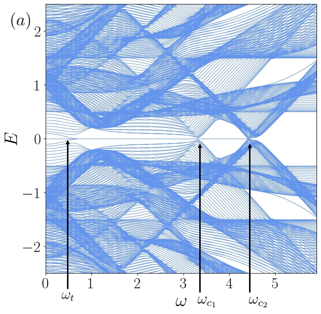
(a) $B<B_{c_{1}}$

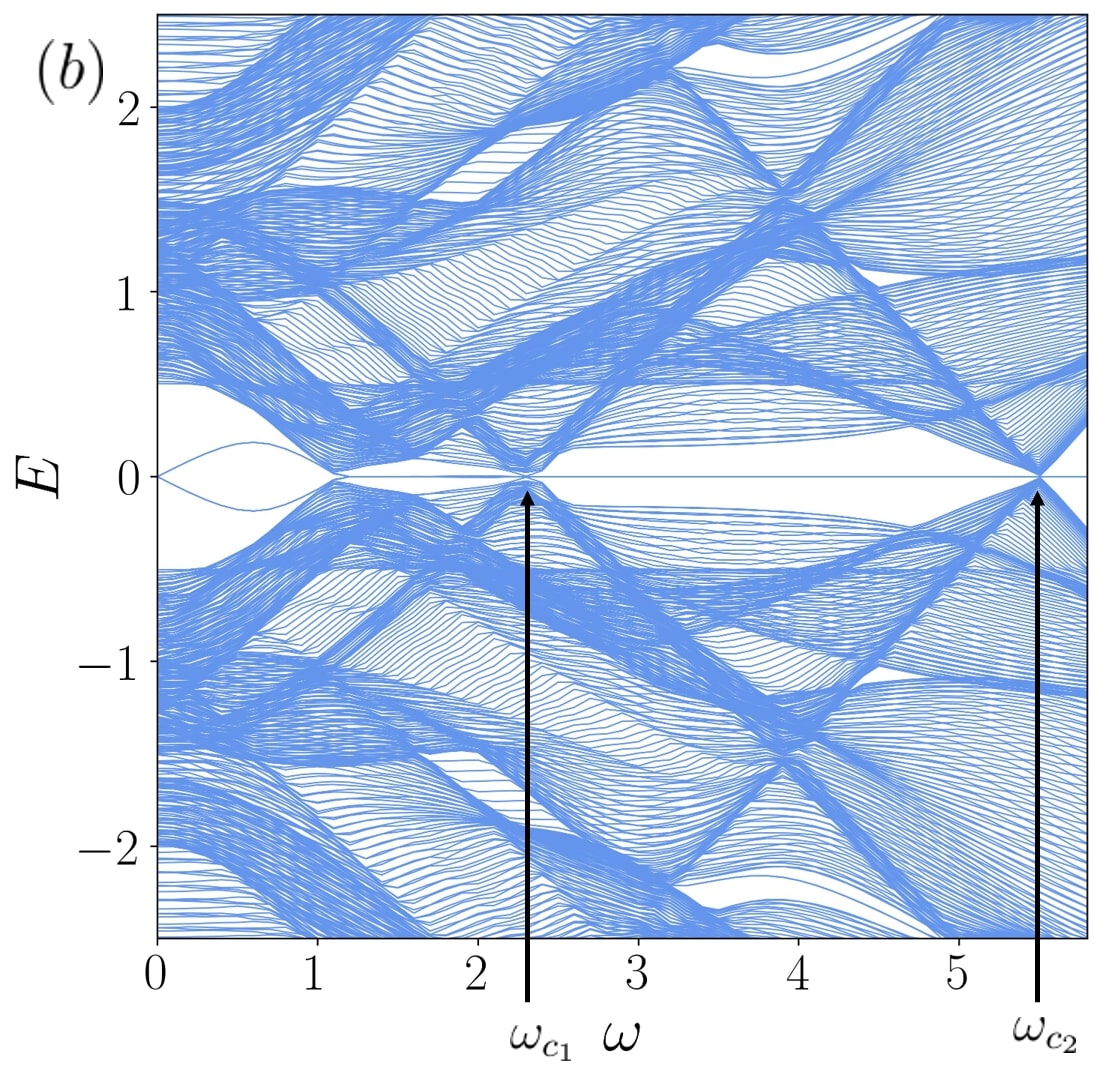
(b) $B_{c_{1}}<B<B_{c_{2}}$

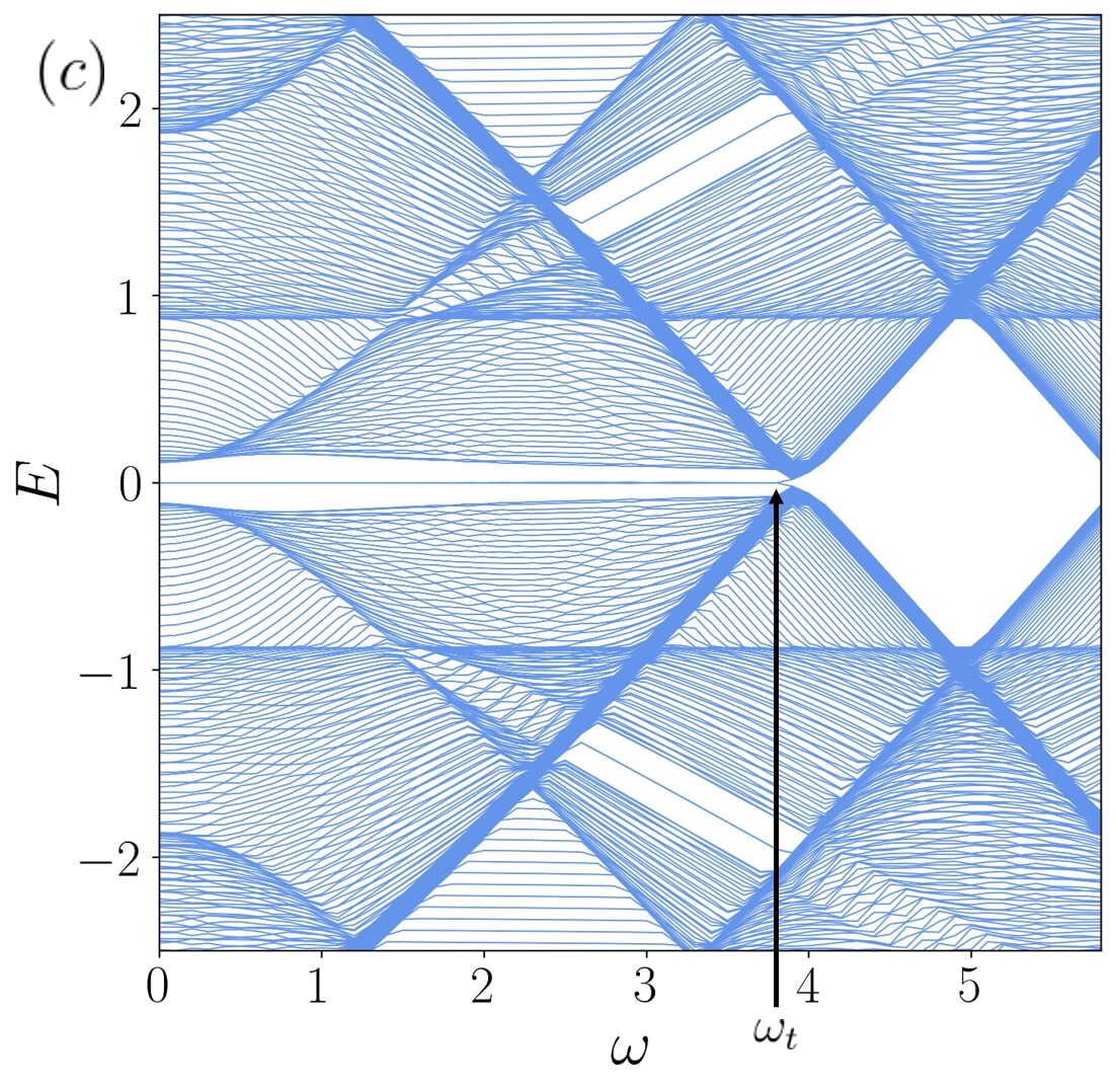
(c) $B>B_{c_{2}}$

Figure 3: The figure depicts real space quasi-energy spectrum (with $m\in[-1,1]$) in the Shirley-Floquet representation plotted as a function of frequency for different magnetic fields. Panel (a) and (c) represent the static trivial limits, $B<B_{c_{1}}$ and $B>B_{c_{2}}$ respectively. Whereas, panel (b) represents the static topological condition, $B_{c_{1}}<B<B_{c_{2}}$. The value of the magnetic fields are chosen as, $B=0.5$ in panel (a), $B=1.5$ in panel (b) and $B=5$ in panel (c). The rest of the parameters are chosen as, $t=1,\mu=0,\Delta=1,B_{1}=1$. properties of the bulk. In Fig. 2a, the dispersion at zero field $(B=0)$ is depicted. It is evident that there are two distinct bands corresponding to different spins: one for particles (at negative energies) and the other for holes (at positive energies). The pairing term, $\Delta$ induces a gap between these bands, while the SOC term, $\alpha$ shifts the two spin bands horizontally. As soon as a magnetic field is switched on with $B<B_{c_{1}}$, for example, $B=0.5B_{c_{1}}$ (see Fig. 2b), the bands do not cross, thereby opening gaps in the spectrum. With further increment in the value of $B$, at $B=B_{c_{1}}$, the outermost bands move further away, whereas the gap between the inner bands closes (see Fig. 2c). As the Zeeman field exceeds this critical value, $B_{c1}$ the spectrum becomes fully gapped again (Fig. 2d). This phenomenon of gap opening and closing signifies a topological phase transition occurring at $B=B_{c_{1}}$, with the topological phase persisting in the region $B_{c_{1}}<B<B_{c_{2}}$. All these results are consistent with previously reported findings [25, 26, 27] and thus lay the groundwork for exploring the driven systems. With this foundation, we are prepared to delve into the Floquet topological characteristics of the periodically driven model, which, in our scenario, manifests through the time-dependent modulation of the magnetic field. To fix our notations, we consider a sinusoidal drive, that is, $H(t)=H_{0}+V_{0}\cos{\omega t}$, with $V_{0}$ and $\omega$, being the amplitude and the frequency respectively of the driving term and $H_{0}$ is a generic static Hamiltonian. The properties of interest in our work can be obtained using Floquet theory [31, 32, 33], according to which, the time-dependent Schrödinger equation can be solved using the Floquet ansatz, $\ket{\psi(t)}=e^{-iEt}\ket{u(t)}$, where $\ket{u(t+T)}=\ket{u(t)}$ denotes the time-periodic Floquet modes, and $E$ represents the Floquet quasi-energies. These Floquet modes can also be interpreted as the eigenstates of Floquet stroboscopic time evolution operator via,

$$\begin{split}&\hat{U}(T)\ket{\psi(0)}=\ket{\psi(T)}\\ &\hat{U}(T)\ket{u(0)}=e^{-iET}\ket{u(T)}=e^{-iET}\ket{u(0)},\end{split}$$ (8)

with the Floquet stroboscopic time evolution operator being,

$$\hat{U}(T)=\mathcal{T}e^{-iH_{\text{eff}}T}.$$ (9)

Here $\mathcal{T}$ denotes the time ordering product and $H_{\text{eff}}$ is the effective time-independent Hamiltonian. One can obtain $E$ and $\ket{u(t)}$ by solving the Floquet-Bloch equation,

$$[H(t)-i\partial_{t}]\ket{u_{k}(t)}=E\ket{u_{k}(t)}.$$ (10)

The operator $H(t)-i\partial_{t}=H_{F}$ is termed as Floquet Hamiltonian. Because of the time periodicity, it is convenient to consider the composite Hilbert space $\mathscr{R}\otimes\mathscr{T}$ where $\mathscr{R}$ is the usual Hilbert space with a complete set of orthogonal basis, and $\mathscr{T}$ is the space of time periodic functions spanned by $e^{-im\omega t}$. This yields the following form of $H_{F}$,

$$H_{F}=\sum_{m,m^{\prime}}\Big{(}m\omega\delta_{m,m^{\prime}}+\frac{1}{T}\int_{0}^{T}dtH(t)e^{-i(m-m^{\prime})\omega t}\Big{)}.$$ (11)

This leads to a situation where we can split the driven spectrum into an infinite number of copies of the undriven Hamiltonian separated by $m\omega$ where, the index $m$ defines a subspace, called as the $m^{th}$ Floquet replica. A general representation of the Floquet Hamiltonian thus can be represented as,

$$H_{F}=\scriptsize{\begin{bmatrix}\ddots&\vdots&\vdots&\vdots&\vdots&\vdots&\iddots\\ \dots&H_{0}-2\omega&H_{-1}&H_{-2}&H_{-3}&H_{-4}&\dots\\ \dots&H_{1}&H_{0}-\omega&H_{-1}&H_{-2}&H_{-3}&\dots\\ \dots&H_{2}&H_{1}&H_{0}&H_{-1}&H_{-2}&\dots\\ \dots&H_{3}&H_{2}&H_{1}&H_{0}+\omega&H_{-1}&\dots\\ \dots&H_{4}&H_{3}&H_{2}&H_{1}&H_{0}+2\omega&\dots\\ \iddots&\vdots&\vdots&\vdots&\vdots&\vdots&\ddots\end{bmatrix}},$$ (12)

where the elements $H_{\pm m}=\frac{1}{T}\int^{T}_{0}{H(t)e^{\pm im\omega t}dt}$ get rid of the explicit time dependence. The Hamiltonian $H_{F}$ is termed as the Shirley-Floquet (SF) Hamiltonian. In the next section, we shall incorporate this method to further study the driven version of our model.

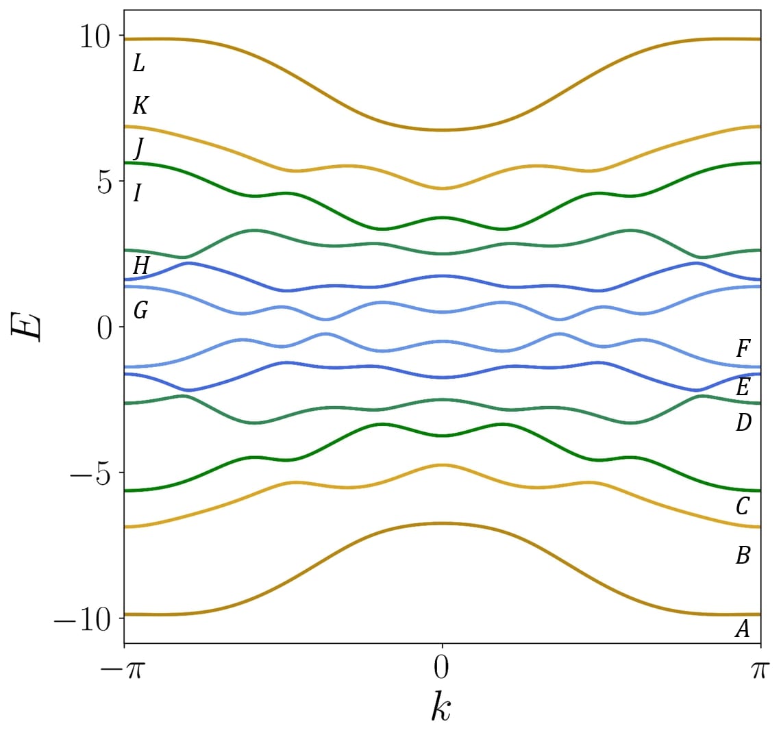
Figure 4: The figure depicts bulk quasi-energy spectrum (with $m\in[-1,1]$) in the Shirley-Floquet representation. The different bands are denoted with letters $A-L$. The rest of the parameters are chosen as, $B_{1}=1$, $\omega=4.5$, and $B=1.5$ (static topological limit).

III Results

III.1 Single-frequency drive

We first describe a harmonic drive, associated with the magnetic field so that Eq. 4 can be rewritten as,

$$\hat{\mathcal{H}}_{z}=\Big{(}B+B_{1}\cos{\omega_{1}t}+B_{2}\cos{\omega_{2}t}\Big{)}\sum_{j}\Big{[}\hat{c}^{\dagger}_{j,\uparrow}\hat{c}_{j,\downarrow}+\hat{c}^{\dagger}_{j,\downarrow}\hat{c}_{j,\uparrow}\Big{]}$$ (13)

The rest of the terms in Eq. 2 are left unaltered. The single drive scenario can be exploited with the conditions, $B_{2}=0$ and $\omega_{1}=\omega$. The Fourier components $|H|_{\pm m}$, except for $m=0,\pm 1$ vanish owing to the mathematical form of the drive. Hence we can truncate the infinite dimensional matrix into a block and can study the corresponding quasi-energy spectrum. By using Floquet theory, we can show that driving induces additional gaps and edge states depending upon the driving frequency and the strength of the driving field. To provide evidence of a topological phase transition in our driven scenario, it is essential to examine the real-space Floquet quasi-energy spectrum across a wide range of frequencies. For benchmarking, fig. 3 illustrates the driven quasi-energy spectrum in both trivial and topological situations, corresponding to the static case. Throughout this paper, we have standardized the energy unit as $t$, the hopping amplitude. The other parameters are chosen as, $\alpha=1,\Delta=1,\mu=0,B_{1}=1$. Upon switching on the time-dependent perturbation, both in the $B<B_{c_{1}}$ and $B>B_{c_{2}}$ regions where the system was entirely trivial in the static case, non-trivial behavior emerges in the presence of driving, accompanied by the appearance of Majorana zero modes (MZMs). Additionally, Majorana $\pi$ modes (MPMs), absent in the static case also manifest. At present, our focus is on the zero-energy modes depicted in Fig. 3 to highlight the distinctions between static trivial and topological limits. Furthermore, multiple gap-closing transitions can be observed, indicating the potential generation of many Majorana modes, which we shall subsequently validate using the topological invariants. By analytically solving the Hamiltonian, we can get three critical values for the driving frequency corresponding to which gap-closing transition occurs. They are,

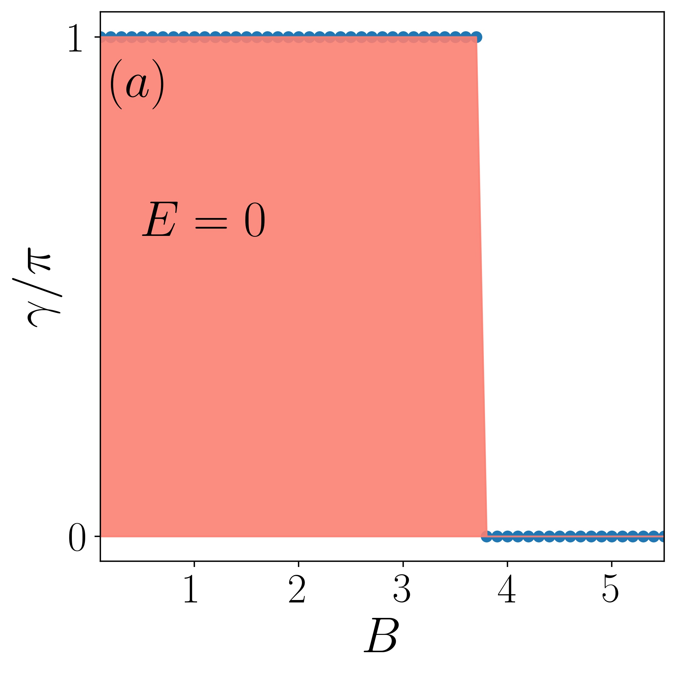
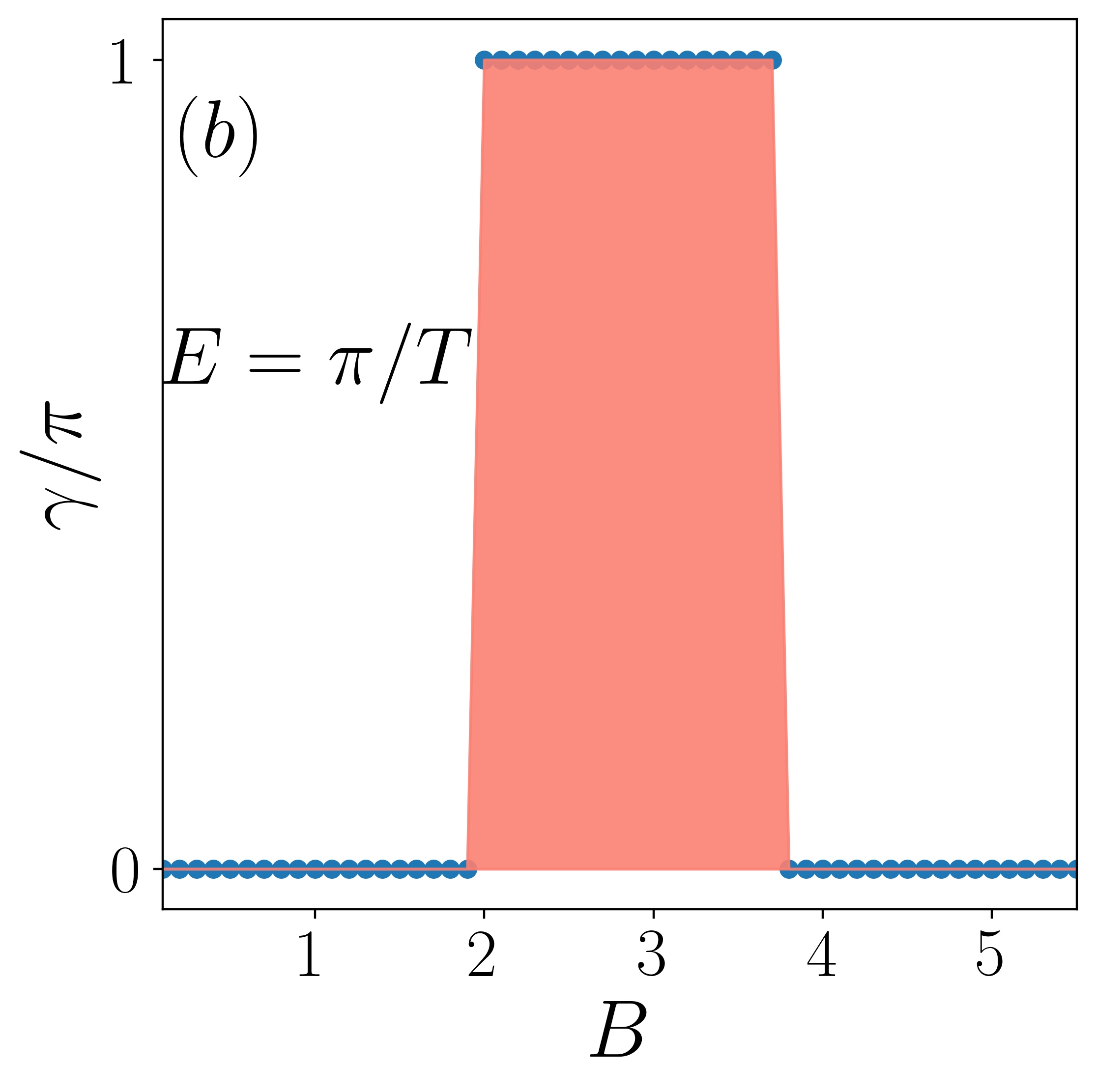
Figure 5: The figures depict total Berry phases for the states filled upto $E=0$ (panel a) and $E=\pi/T$ (panel b), as a function of the driving frequency, $\omega$ in the static trivial limit, $B>B_{c_{2}}$. The results correctly match with the real space quasi-energy spectrum shown in Fig. 3.

$$\omega_{c_{1}}=-B+\sqrt{(\mu-4t)^{2}+\Delta^{2}}$$ (14a)

$$\omega_{c_{2}}=B+\sqrt{(\mu-4t)^{2}+\Delta^{2}}$$ (14b)

$$\omega_{t}=-B+\sqrt{\mu^{2}+\Delta^{2}}$$ (14c)

The gap closes at the center of the FBZ ($k=0$) corresponding to $\omega=\omega_{t}$, and at the edges of the FBZ ($k=\pm\pi$) for $\omega=\omega_{c_{1},c_{2}}$. These conditions for the closure of the bulk gap serve to delineate the boundaries of the topological phases, as illustrated in Fig. 3. For instance, in Fig. 3a, for $B=0.5$, within the static trivial limit ($B<B_{c_{1}}$), the zero-energy modes persist up to $\omega=\omega_{c_{2}}=4.5$ It is important to note that there are instances of gap closing, although not directly linked to the topological phase transition, however can result in the emergence of multiple Majorana modes. For example, in Fig. 3a, the MZMs experience an additional gap-closing transition at $\omega=\omega_{c_{1}}=3.5$ followed by another transition at $\omega=\omega_{t}=0.5$, both of which does not impact its topological phase. On the other hand, for $B=1.5$ (Fig. 3b), corresponding to static topological limit ($B_{c_{1}}<B<B_{c_{2}}$), MZMs appear beyond $\omega=\omega_{c_{1}}=2.5$ and undergo another gap closing transition at $\omega=\omega_{c_{2}}=5.5$, indicating an increase in the number of Majorana modes. Additionally, there are instances of gap closing for example, in Fig. 3b $\omega\approx 1$, corresponds to a bulk gap closure at some non-high symmetric points ($k\neq 0,\pm\pi$). Finally, in Fig. 3c for $B=5$, corresponding to static trivial limit ($B>B_{c2}$), the MZMs persist upto a frequency, $\omega=\omega_{t}$. However, in this scenario, there occurs only one gap-closing transition. Hence, based on the preceding discussions, we can infer that in the static non-trivial range, $B_{c_{1}}<B<B_{c_{2}}$, the driven system exhibits MZMs in the high-frequency regime ($\omega>\omega_{c_{2}}$). Whereas, in the static trivial range for $B<B_{c_{1}}$ and for $B>B_{c_{2}}$, the driven system showcases MZMs in the low-frequency regime, namely, $\omega<\omega_{c_{1}}$ and $\omega<\omega_{t}$ respectively but not in the high-frequency regime.

To validate the topological characteristics alongside the ‘bulk-edge correspondence’, we compute the topological invariant [80]. In the frequency domain, the pertinent invariant for a $3\times 3$ Floquet-Bloch Hamiltonian is the Berry phase [81, 82, 83], that denotes the geometric phase accrued by a wave function during a smooth traversal across the Brillouin zone. The Berry phase is defined as,

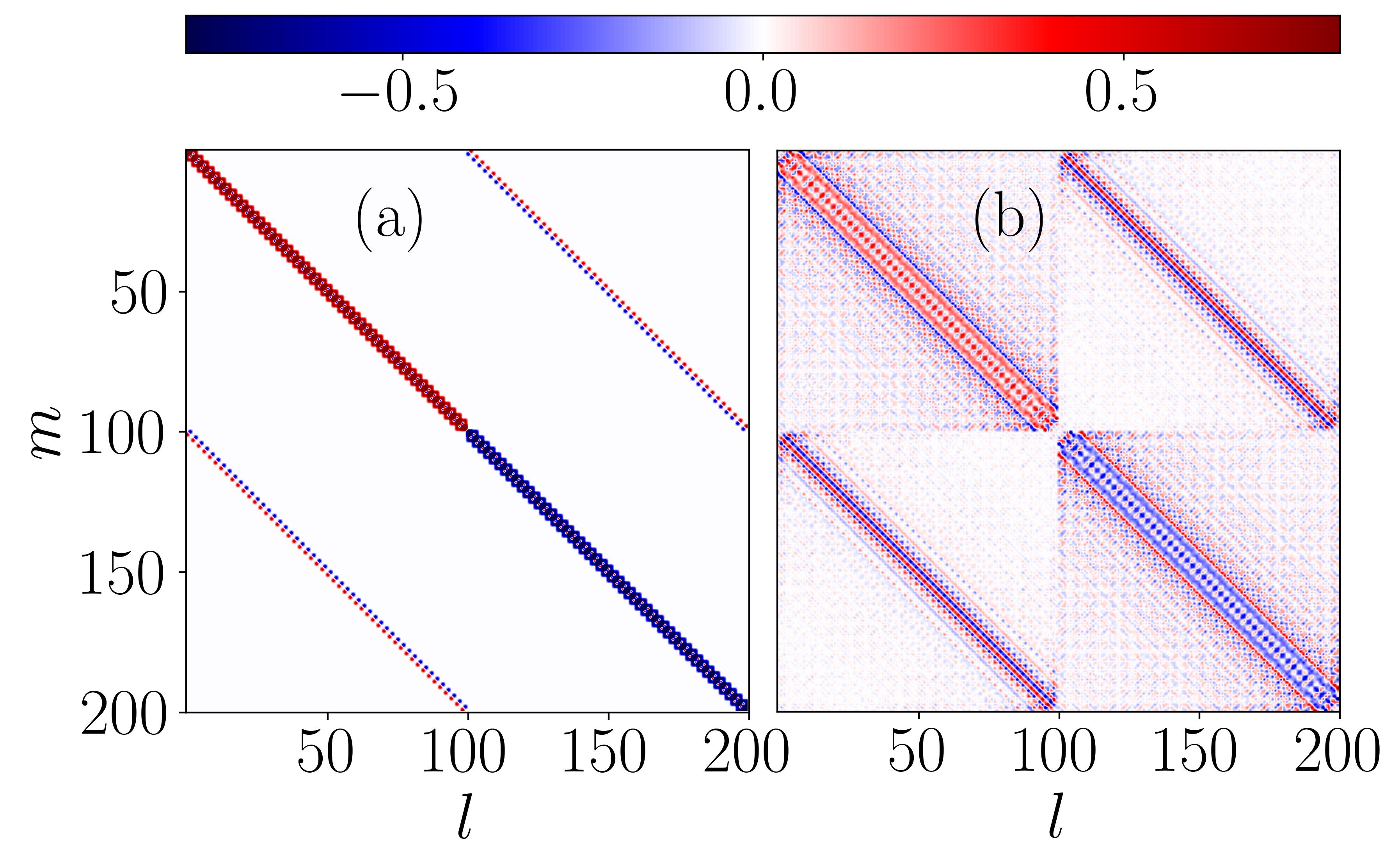
Figure 6: Figure depicts the expansion coefficients for both static (panel a) and driven (panel b) Hamiltonian in the occupation basis ($c_{1,\uparrow}^{\dagger},c_{1,\downarrow}^{\dagger},...c_{N,\downarrow}^{\dagger},c_{1,\uparrow},c_{1,\downarrow},...c_{N,\downarrow}$), where $l$ and $m$ denotes the base indices. The results clearly indicates the induction of longer-range interactions. The rest of the parameters are chosen as, $B_{1}=1$, $B=1.5$, and $\omega=2$.

$$\gamma=i\oint dk\langle{u_{k}}|\nabla_{k}{u_{k}}\rangle,$$ (15)

where $\ket{u_{k}}$ are the Bloch states. A Hamiltonian exhibiting a non-trivial Berry phase cannot be adiabatically linked to an atomic insulator unless a gap-closing transition takes place. The numerical calculation of the Berry phases $\gamma_{\beta}$ corresponding to different bands ($\beta$ denotes the band index, marked with the letters $A-L$ in Fig. 4) for a particular frequency, say, $\omega=4.5$, is obtained as,

$$\gamma_{\beta}=\begin{cases}0\quad(\beta=B,C,D,E,H,I,J,K)\\ \pi\quad(\beta=F,G)\\ \end{cases}\textrm{for}~{}B<B_{c_{1}},$$ (16)

$$\gamma_{\beta}=\begin{cases}\pi\quad(\beta=F,G)\\ 0\quad(\beta=B,C,D,E,H,I,J,K)\\ \end{cases}\textrm{for}~{}B>B_{c_{1}}.$$ (17)

The outermost bands, that is, $\beta=A~{}\text{and}~{}L$ always contribute to zero Berry phase, since they do not participate in the band inversion process. It is noteworthy that there is at least one band below the Fermi level exhibiting a non-zero Berry phase, indicating that the system is in a topologically non-trivial state. One can also verify that the combined sum of Berry phases given by, $\gamma=|\textrm{mod}(\sum_{\beta}\gamma_{\beta},2)|$, below an energy zero or $\pm\pi/T$ energy correlates with the edge modes identified in the real-space spectrum. For example, Fig. 5 illustrates the cumulative sum of Berry phases up to $E=0$ (Fig. 5a) and $E=\pi/T$ (Fig. 5b) respectively corresponding to one of the static trivial conditions, namely, $B>B_{c_{2}}$. These correctly anticipate the appearance of zero and $\pi$ energy modes as already depicted in Fig. 3c.

Though the Berry phase provides insights into the emergence of Majorana zero and $\pi$ energy modes, it cannot precisely quantify the number of each of these localized edge modes. Consequently, we turn to calculating the particular invariant associated with the static version of the model, which as stated earlier falls in the symmetry class D which is characterized by a $\mathbb{Z}_{2}$ invariant. Thus, one should obtain only one pair of Majorana modes. The scenario raises doubts about the multiple gap-closing transitions observed and the prediction of many Majorana modes, as obtained by us here. This prompts a speculation regarding its origin. Could it be the emergence of longer-range interactions into the driven system? This leads to one of the key results and shows the richness of the non-equilibrium phenomena embedded in our model. In order to validate our concern, we focus on diagonalizing the stroboscopic time evolution operator, $\hat{U}(T)$ introduced in Eq. 9. In Fig. 6, we present the expansion coefficients of $H_{\text{eff}}$ in the occupation basis ($c_{1,\uparrow}^{\dagger},c_{1,\downarrow}^{\dagger},...c_{N,\downarrow}^{\dagger},c_{1,\uparrow},c_{1,\downarrow},...c_{N,\downarrow}$) corresponding to a particular frequency, namely, $\omega=2$, in order to compare and contrast it with the expansion coefficient for the static scenario illustrated in Fig. 6a. The analysis indicates a clear distinction, the coefficients in the driven scenario reveal evidence of longer-range (spanning over

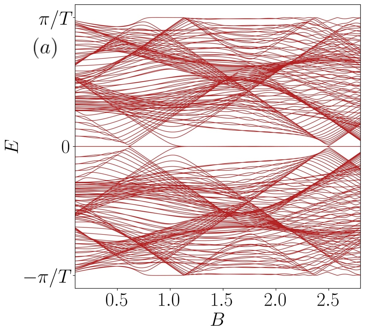
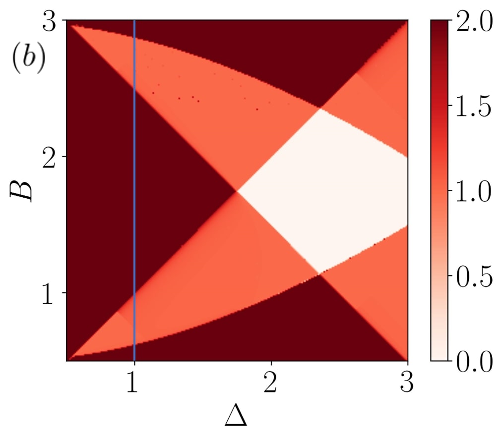
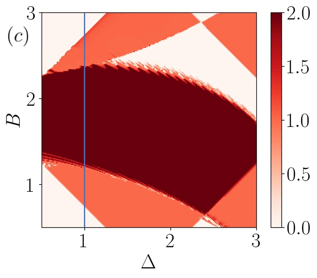
Figure 7: Panel (a) shows the Floquet quasi-energy spectrum confined within the FBZ, plotted as a function of the strength of the magnetic field, $B$ with a fixed pairing strength, $\Delta=1$. Panel (b)-(c) depict the topological phase diagram in the $B-T$ plane, computed using the winding numbers corresponding to the zero $(\nu^{0})$ and the $\pi$ ($\nu^{\pi}$) energy modes respectively. The rest of the parameters are chosen as, $B_{1}=1,\omega=3.5$. more than 10 sites) interactions (Fig. 6b). Moreover, as the frequency decreases, more longer-range interactions emerge in the driven system. The way one can reconcile this is to do a Baker-Campbell-Hausdorff (BCH) expansion where the nested commutator brackets induce coupling between distant sites which yields more off-diagonal terms in $\hat{U}(T)$ leading to the generation of many Majorana modes. subsequently, we shall address this issue by leveraging all the symmetries inherent in the evolution operator, $\hat{U}(T)$, which can be split into a pair of symmetric frames, enabling the determination of the topological invariant associated with the driven model. To determine such an invariant for a 1D Hamiltonian, one can compute the winding number, which is defined as,

$$\nu[h]=\frac{1}{2\pi i}\int_{BZ}dk\frac{d}{dk}\log{h(k)}.$$ (18)

Mathematically, the winding number assumes the same information as the Berry phase. However, determining the winding number entails the Hamiltonian to adopt an off-diagonal form in the canonical basis, where $\hat{C}$ is diagonal. This, for our $\mathcal{H}(k)$ reads as,

$$\hat{S}^{\dagger}\mathcal{\hat{H}}(k)\hat{S}=\begin{pmatrix}0&A(k)\\ A^{\dagger}(k)&0\\ \end{pmatrix},$$ (19)

where $A(k)$ is a $2\times 2$ Hermitian matrix. Further, $\hat{S}$ is a unitary matrix constructed using the particle-hole basis,

$$\hat{S}=\frac{1}{\sqrt{2}}\begin{pmatrix}\sigma_{x}&\sigma_{x}\\ -\sigma_{y}&\sigma_{y}\\ \end{pmatrix}$$ (20)

Finally, one can rewrite the definition of the winding number corresponding to our case as,

$$\nu=\frac{-1}{2\pi i}\oint dk\frac{d}{dk}\ln{det|A|}.$$ (21)

One may pause here and review the choice of the time frame chosen. For example, a different choice for the period may lead to certain $\hat{U}(T)$, which may not have any symmetries and will make the formalism ineffective. Further, the energy spectra of the Hamiltonian corresponding to $\hat{U}(T)$ is plotted in Fig. 7a which distinctly yield multiple gap closing transitions, and hence multiple Majorana modes. To confirm the presence of such multiple Majorana scenario, a pair of bulk invariants are required. To address this, we employ the concept of ‘pairs of symmetric time frames’ [84, 85]. To ensure all symmetries of the driven system, we require a time that splits the period into two symmetrical parts. Let $\hat{F}$ and $\hat{G}$ denote the time evolution of the first and second parts respectively, then in one of the symmetric time frames, the evolution operator, $\hat{U}(T,0)$ takes the form, $\hat{U}=\hat{F}\hat{G}$. It is also easy to ascertain that if there is a symmetric frame for a Floquet evolution operator $\hat{U^{\prime}}=\hat{F}\hat{G}$, then another symmetric time frame corresponding to the Floquet evolution operator $\hat{U^{\prime\prime}}=\hat{G}\hat{F}$ must also exist. However, neither of these frames individually offers complete insight into the number of edge modes. Rather, based on the periodic table of Floquet topological insulators and superconductors [86], they need to be combined in a specific way so that each nontrivial phase can be identified by a pair of noncommutative winding numbers given as,

$$\nu^{0}=\frac{\nu^{\prime}+\nu^{\prime\prime}}{2}\quad;\quad\nu^{\pi}=\frac{\nu^{\prime}-\nu^{\prime\prime}}{2}.$$ (22)

Here $\nu^{\prime}$ and $\nu^{\prime\prime}$ are the winding numbers for the two effective Hamiltonians corresponding to the two symmetric time frames $\hat{U^{\prime}}$ and $\hat{U^{\prime\prime}}$ respectively.

Fig. 7 shows the topological phase diagrams in $B-\Delta$ plane, plotted for certain values of $\omega$ and $B_{1}$ such that, $\omega=3.5$, and $B_{1}=1$. To confirm the bulk-edge correspondence, one can compare the outcomes with the real-space quasi-energy spectrum plotted as a function of $B$ for $\Delta=1$ (Fig. 7a). A noteworthy observation from Figs. 7a,b is the coexistence of zero and $\pi$ Majorana modes in certain regions of the parameter space. A recent investigation [53, 54] demonstrated that this superposition of zero and $\pi$ edge states leads to a novel type of symmetry-protected discrete time crystal phase, referred to as ‘period-2$T$ Floquet time crystal phase’, offering new possibilities for non-Abelian braiding and topological quantum computing in superconducting Floquet systems. Consequently, higher values of the winding number at same values of the parameters obtained here could suggest the potential for generating multiple Floquet time crystals.

III.2 Multi-frequency drive

III.2.1 Commensurate case

Here, we present the method for the treatment of Eq. 13 corresponding to a two-tone commensurate driving setup with $B_{2}\neq 0$. The periodicity of the two drives, $T_{1}$ and $T_{2}$ may obey following equation,

$$\frac{T_{1}}{T_{2}}=\frac{n_{2}}{n_{1}},$$ (23)

implying that one may always find a common time period $T$, such that,

$$T=n_{1}T_{1}=n_{2}T_{2}$$ (24)

which will further be used to employ the Floquet theory.

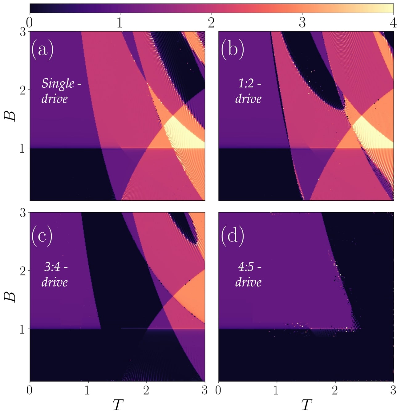
Figure 8: The figure depicts topological phase diagrams concerning MZMs for single-drive scenario (panel a) and for various multi-frequency driving scenario. For example, we study the case of a 1:2 drive in panel (b), 2:3 drive in panel (c), and a 4:5 drive in panel (d). the strength of the two drives are chosen as, $B_{1}=B_{2}=1$.

At first, we shall investigate the impact of the second drive while keeping the strength of the first drive constant, with a ratio of the frequencies being, $n_{1}:n_{2}=1:2$. This choice of bichromatic driving is considered experimentally feasible and has been demonstrated to possess adjustable sensitivity [73].

It is worth noting that, maintaining the first drive constant, results in minimal alterations to the nature associated with the $\pi$ modes, especially in the high-frequency region. Therefore, our subsequent discussion will concentrate on the evolution of zero modes under two-tone commensurate driving across different frequency regimes. In Fig. 8, we have illustrated topological phase diagrams showing the distribution of zero energy modes across the $B-T$ plane. To ensure a smooth comparison, the single-drive scenario has been included as well. Upon analysis of these figures, notable findings emerge. For instance, regions that appeared topologically trivial in Fig. 8a now exhibits non-trivial behavior with the inclusion of an additional drive (Fig. 8b), and the converse is true as well. Furthermore, we have included results regarding other commensurate multi-tone driving protocols, where the ratios of integers are not uniquely expressed as an integer multiple, such as $n_{1}:n_{2}$ = 3:4 (Fig. 8c) and $n_{1}:n_{2}$ = 4:5 (Fig. 8d) to encompass complex driving scenarios. It is evident that such intricate driving patterns tend to populate the spectrum more densely, leading to quasi-energy spectra that are denser and thus reducing the bulk gap compared to that of the single-drive and 1:2 cases. Consequently, lesser number of localized edge modes appear to be shielded by a finite bulk gap, thereby shrinking the range of non-trivial phases. Moreover, even in Fig. 8d, corresponding to a 4:5 driving protocol, the system has no longer access to higher winding numbers. Nonetheless, regardless of the different driving protocols, they all lead to very similar gap closure and hence the same winding numbers are obtained in the $B-T$ plane, specifically in the region where $(B,T)\leq(1.5,1.5)$. The alteration in the winding number only occurs at higher values of magnetic field, $B$, and the time period, $T$.

From the preceding discussions, it is clear that the localization of the edge modes is significantly influenced by the chosen driving protocol. Even with complex driving scenarios (where the integers are not uniquely expressed as integer multiples), the Majorana modes lose their characteristic localization behavior and manifest as extended states. Thus, it is conceivable to manipulate the stability and presence of the edge modes by conveniently switching between different driving protocols. This could prove beneficial in quantum computation setup comprising of multiple interconnected segments of Kitaev chains [87]. The experimental advantage lies in the ability to selectively alter the localization of the edge modes without changing the static parameters of the model. As a result, one could apply this multi-tone driving strategy to a network of Kitaev chain segments, where the parameters of each segment may be beyond controllable due to practical limitations. It is worth mentioning that the bichromatic driving protocol can also be examined using the Shirley-Floquet approach, as previously discussed in Sec.II. However, truncating the infinite-dimensional matrix will now depend on the ratio of the driving frequencies. Consequently, corresponding to a complex driving scenario utilizing this formalism and performing associated computations could appear to be cumbersome [74].

III.2.2 Incommensurate case

In this section, we shall explore the implications on topology when the Rashba nanowire model with topological superconductivity is subjected to an incommensurate multi-frequency driving protocol, where the ratio $n_{1}:n_{2}$ is no longer a rational number. For instance, let us consider the case where $n_{1}:n_{2}=\beta$, where $\beta=(\sqrt{5}+1/2)$, represents the golden ratio, defined as the ratio between two successive large numbers in the Fibonacci series. Consequently, with no global time periodicity, the conventional stroboscopic Floquet operator cannot be defined. To address this, we shall utilize the framework established by Ho et al. in Ref. [76, 77, 78, 79], also referred to as the many-mode Floquet theory (MMFT). By utilizing the Shirley-Floquet approach as a foundation, one can set up the formalism by relabelling the basis vectors in the Shirley’s framework to construct an extended basis vector derived from the tensor product of the two Fourier spaces. That is,

$$\ket{m}\rightarrow\ket{m_{1}}\otimes\ket{m_{2}},$$ (25)

with the initial condition being, $m\omega=m_{1}\omega_{1}+m_{2}\omega_{2}$ or equivalently, $m=n_{1}m_{1}+n_{2}m_{2}$, where $m_{1},m_{2}$ are two integers. Based on the formalism elucidated in Sec.II, the multi-frequency time-dependent problem can be mapped to an equivalent time-independent eigenvalue problem given as,

$$\begin{split}\bra{m_{1},m_{2}}H_{F}\ket{m_{1}^{\prime},m_{2}^{\prime}}=&(m_{1}\omega_{1}+m_{2}\omega_{2})\delta_{(m_{1},m_{1}^{\prime})}\delta_{(m_{2},m_{2}^{\prime})}\\ &+\mathcal{H}_{(m_{1}-m_{1}^{\prime}),(m_{2}-m_{2}^{\prime})},\end{split}$$ (26)

where,

$$\begin{split}\mathcal{H}_{(m_{1}-m_{1}^{\prime}),(m_{2}-m_{2}^{\prime})}=&\sum_{i=1}^{2}[V_{1,2}](\delta_{m_{i},1}+\delta_{m_{i},-1})\\ &+E\delta_{m_{1},0}\delta_{m_{2},0}\end{split}$$ (27)

and,

$$V_{1,2}=\frac{1}{T_{1,2}}\int_{0}^{T_{1,2}}dt\mathcal{H}_{z}(t)e^{-i(m_{1,2}-m_{1,2}^{\prime})\omega_{1,2}t}.$$ (28)

In matrix notation, $H_{F}$ reads as, $$H_{F}={\begin{bmatrix}\ddots&\vdots&\vdots&\vdots&\vdots&\vdots&\iddots\\ \dots&A-2\omega_{2}&B&0&0&0&\dots\\ \dots&B&A-\omega_{2}&B&0&0&\dots\\ \dots&0&B&A&B&0&\dots\\ \dots&0&0&B&A+\omega_{2}&B&\dots\\ \dots&0&0&0&B&A+2\omega_{2}&\dots\\ \iddots&\vdots&\vdots&\vdots&\vdots&\vdots&\ddots\end{bmatrix}},$$ (29) where, $$A={\begin{bmatrix}\ddots&\vdots&\vdots&\vdots&\vdots&\vdots&\iddots\\ \dots&H_{0}-2\omega_{1}&V_{1}&0&0&0&\dots\\ \dots&V_{1}&H_{0}-\omega_{1}&V_{1}&0&0&\dots\\ \dots&0&V_{1}&H_{0}&V_{1}&0&\dots\\ \dots&0&0&V_{1}&H_{0}+\omega_{1}&V_{1}&\dots\\ \dots&0&0&0&V_{1}&H_{0}+2\omega_{1}&\dots\\ \iddots&\vdots&\vdots&\vdots&\vdots&\vdots&\ddots\end{bmatrix}},\quad\text{and}\quad B={\begin{bmatrix}\ddots&\vdots&\vdots&\vdots&\vdots&\vdots&\iddots\\ \dots&V_{2}&0&0&0&0&\dots\\ \dots&0&V_{2}&0&0&0&\dots\\ \dots&0&0&V_{2}&0&0&\dots\\ \dots&0&0&0&V_{2}&0&\dots\\ \dots&0&0&0&0&V_{2}&\dots\\ \iddots&\vdots&\vdots&\vdots&\vdots&\vdots&\ddots\end{bmatrix}}$$ (30) Note that the matrix $A$ is nothing but the SF Hamiltonian corresponding to the single drive scenario.

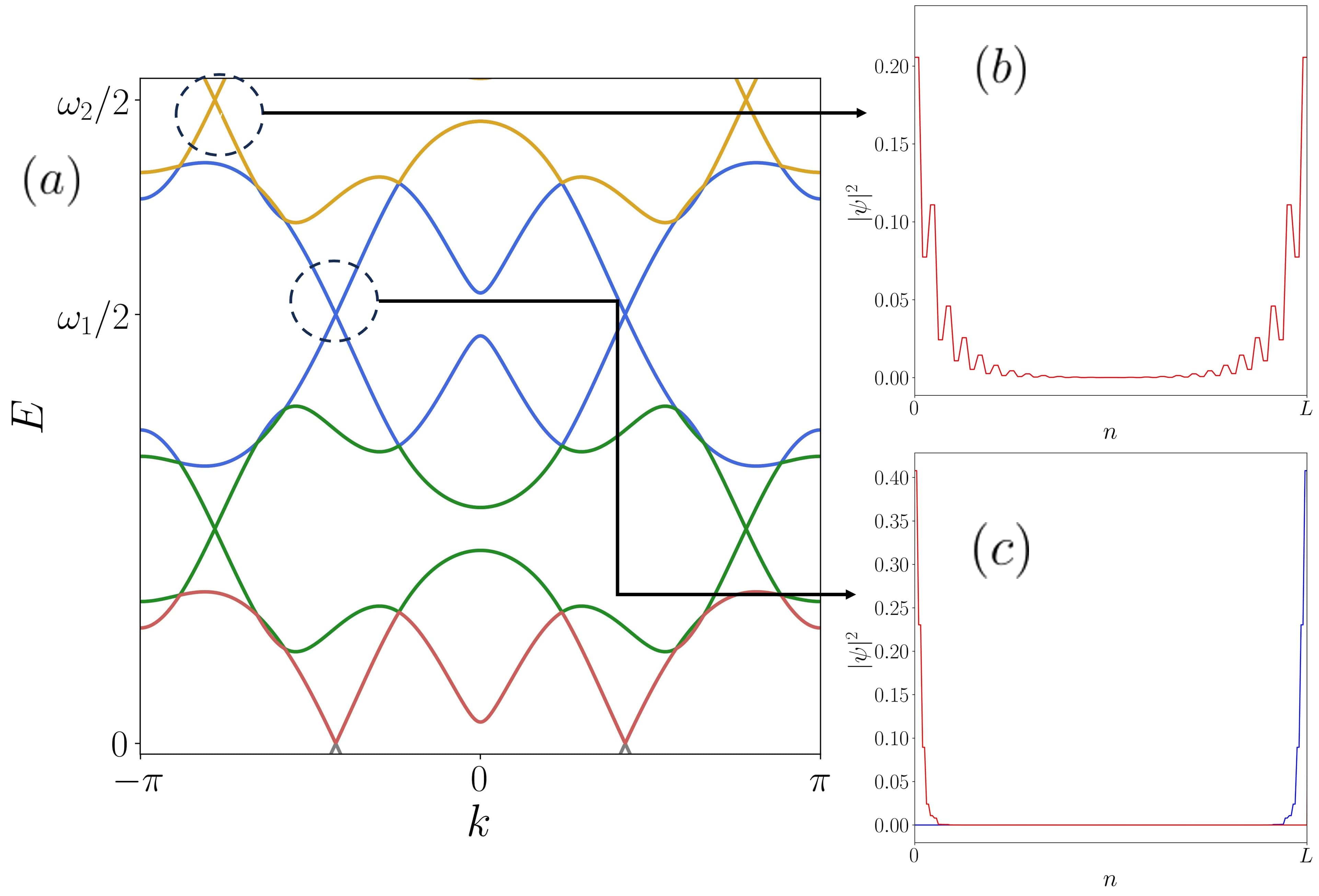
Figure 9: Panel (a) depicts the bulk quasi-energy spectrum corresponding to an incommensurate multi-frequency driving protocol in the static topological limit ($B=1.5$). There are two distinct level crossings at energy, $E=\omega_{1}/2$, and $E=\omega_{2}/2$. As soon as the time-dependent perturbation is switched on, a gap appears at these points. Panel (b) and (c) represent the probability distributions of these two Majorana states plotted as a function of the site index, $n$. The ratio of the two frequencies has been chosen as, $\omega_{2}/\omega_{1}=\beta=\sqrt{5}+1/2.$ The strength of the two drives are fixed at, $B_{1}=B_{2}=1$.

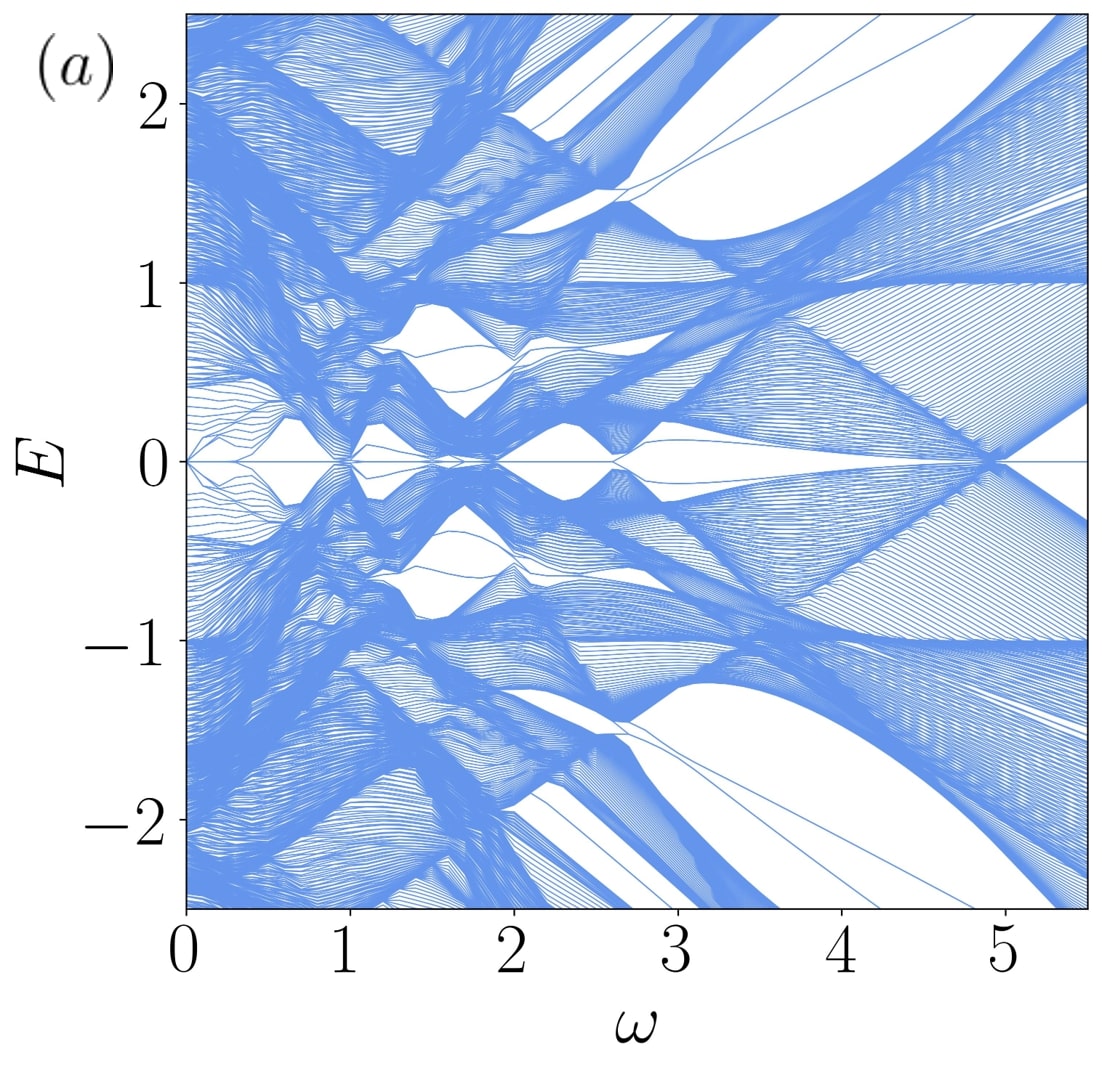
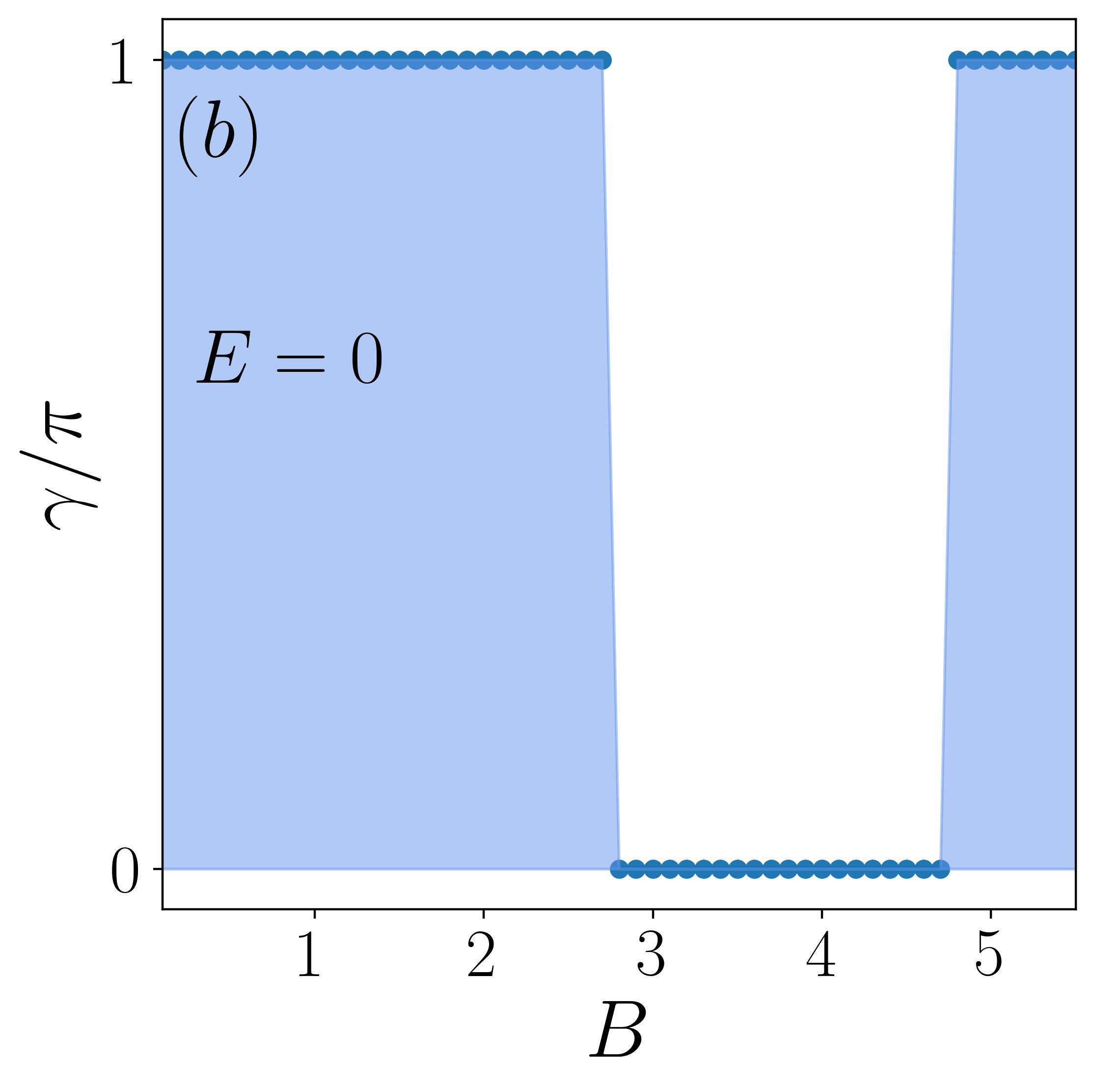
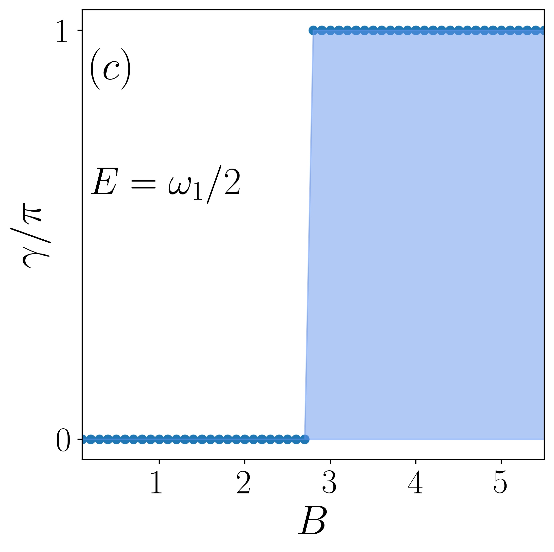
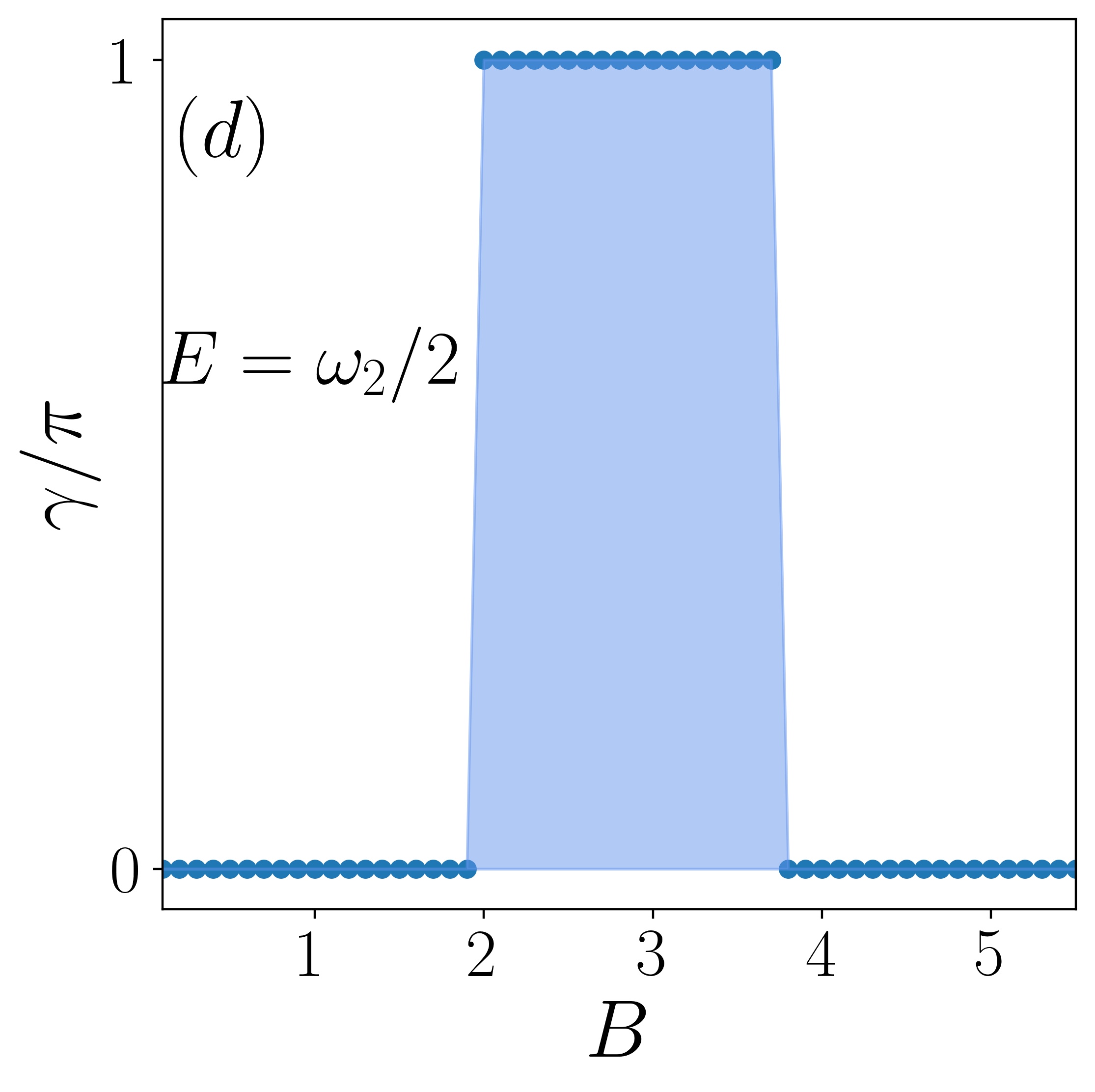
Figure 10: Panel (a) represents the real-space quasi-energy spectrum in the many-mode Floquet formalism corresponding to an incommensurate multi-frequency driving protocol in the static topological limit ($B=1.5$). Panel (b)-(d) are the total Berry phases of the states filled upto $E=0$, $E=\omega_{1}/2$, and $E=\omega_{2}/2$ respectively. The ratio of the two frequencies has been chosen as, $\omega_{2}/\omega_{1}=\beta=\sqrt{5}+1/2.$ The strength of the two drives are fixed at, $B_{1}=B_{2}=1$.

This mechanism bears resemblance to the treatment outlined in Ref. [66], where the interplay among various incommensurate drives is explored within a multidimensional Fourier space by effectively introducing synthetic dimensions. Consequently, dealing with any model in 1D may necessitate a 3D computation (its own dimension and the two corresponding to the two frequencies). Furthermore, employing two competing truncation schemes of the Fourier space may lead to additional complexities. Therefore, it would be beneficial to approximate our findings using the 1D MMFT proposed herein. Moreover, the effective field $\vec{m}\cdot\vec{\omega}$ can be interpreted as a Wannier-Stark field indicating the absorption or emission of energy from the drive in terms of the integers, $m_{1}$ and $m_{2}$. Furthermore, since $\vec{m}\cdot\vec{\omega}=m_{1}\omega_{1}+m_{2}\omega_{2}$ can be seen to yield any arbitrary energy increment along both $m_{1}$ and $m_{2}$, the quasi-energy spectrum gets densely populated everywhere. Consequently, it appears that the Majoranas lack a protective cover to prevent them from hybridizing into the bulk. Nevertheless, these Majoranas remain stable and robust against local perturbations owing to the Wannier-Stark localization along the $\vec{m}\cdot\vec{\omega}$ direction and due to the quasiperiodicity induced in the Floquet space. Moreover, the interplay between the two mutually incommensurate drives can lead to the emergence of various types of $\pi$ Majorana modes, as evidenced by the presence of two distinct level crossings at energies, $E=\omega_{1}/2$ and $E=\omega_{2}/2$ (Fig. 9a, where the gap closes at two different $k$ values, shown by the dashed circles). In an open chain, as soon as the time-dependent perturbation is switched on, these could give rise to the emergence of distinct localized edge states (shown in Figs. 9b,c). Furthermore, the appearance of these unique $\pi$ modes can be regulated independently due to the fact that by keeping one drive constant while setting the other to be zero, it is possible to switch between different bulk gaps. For instance, starting with $B_{2}=0$ and $B_{1}\neq 0$, the gap opens solely at $E=\omega_{1}/2$, and when $B_{2}\neq 0$ and with finite $B_{1}$, the gap opens at $E=\omega_{1}/2$. The existence and stability of the Majoranas have been affirmed through the analysis of the probability distribution corresponding to the eigenstates (Figs. 9b,c). Additionally, the localization of these novel Majorana modes in the drive-induced synthetic dimensions has been investigated in Ref. [68]. As predicted, unlike the gapped Floquet topological phase, the quasi-energy spectra of a time-quasiperiodic system are uniformly dense. In Fig. 10a, we illustrate the real-space quasi-energy spectra corresponding to three replicas in each of the frequency direction for a magnetic field, namely, $B=1.5$. Even in a magnified version, the quasi-energy spectra are densely packed, making it difficult to discern the various Majorana modes. Unlike the situation in the commensurate case, we cannot establish a winding number because of the inability to define a stroboscopic time evolution operator. Instead, similar to the Shirley-Floquet approach, different Majoranas can be characterized using the Berry phase. In Figs. 10(c-d), we have plotted Berry phases corresponding to $0,\omega_{1}/2$, and $\omega_{2}/2$ Majorana modes by taking the cumulative sum of the phases corresponding to the bands below energies, $E=0,\omega_{1}/2$, and $\omega_{2}/2$ respectively. It is noteworthy that there are regions in the parameter space where all these Majoranas can coexist independently of each other. As a consequence, this could offer potential applications for tunable control over accessing localized edge states. For instance, Instead of relying on several static topological superconducting wires, one can dynamically produce multiple Majoranas at various locations of the same network. This presents an intriguing avenue for future exploration, potentially opening up opportunities to investigate diverse Floquet time crystalline phases. It would be valuable to examine how the period doubling gets affected due to the simultaneous presence of distinct Majorana modes.

IV Conclusion

In summary, this paper explores a feasible topological superconductor model involving a Rashba nanowire subjected to multiple driving forces, aiming to generate numerous and novel Majorana modes. By leveraging the topological phase boundaries of the undriven model, we confirm the presence of distinct non-trivial characteristics at certain frequency limits. For instance, corresponding to the static trivial (topological) limits, the Majorana zero modes appear only at low (high) frequency regimes. Additionally, the non-trivial nature of the system is validated through the computation of several bulk invariants, such as the Berry phase associated with the Shirley-Floquet formalism. Further, the periodic drive induces longer-range interactions, leading to the generation of multiple Majorana modes where there is a possible alteration of the symmetry classification. By exploiting the symmetries associated with the Floquet stroboscopic operator, we have been able to classify the effective Hamiltonian via a pair of bulk invariants that uniquely predict the emergence of both zero and $\pi$ Majorana modes. Later, the inclusion of an additional drive leads to intriguing results that could have potential applications in quantum computation and time crystals. Within a commensurate driving scheme, the ability to dynamically manipulate the generation and stability of the edge modes are feasible by carefully choosing a suitable multi-frequency driving protocol. This results in a diverse range of edge states that exhibit varying degrees of localization, spanning from highly localized to fully delocalized ones. Moreover, more intricate driving protocols tend to populate the spectrum more densly and diminish the size of the quasienergy gaps, leading to the delocalization of the edge modes. Thus, by switching between various driving protocols, one can gain dynamical control over the presence and robustness of Majorana modes. However, in an incommensurate driving scheme, the absence of global time periodicity prevents the definition of usual stroboscopic evolution operator, limiting our analysis to the frequency space. Nevertheless, similar to Shirley’s formalism, we have effectively addressed the problem in an extended frequency domain. This leads to the emergence of distinct Majorana modes not located at $E=0$, rather at $E=\omega_{1}/2,$ and $E=\omega_{2}/2$. As a result, the simultaneous existence of time-quasiperiodic Majoranas could offer opportunities for exercising control over quantum computation by accessing multiple Majoranas at various locations within the same network.

References

- [1] K. v. Klitzing, G. Dorda, and M. Pepper, Phys. Rev. Lett. 45, 494 (1980).
- [2] S. Ryu and Y. Hatsugai, Phys. Rev. Lett. 89, 077002 (2002).
- [3] M. Z. Hasan and C. L. Kane, Rev. Mod. Phys. 82, 3045 (2010).
- [4] X.-L. Qi and S.-C. Zhang, Rev. Mod. Phys. 83, 1057 (2011).
- [5] J. E. Moore, Nature 464, 194 (2010).
- [6] A. Bansil, H. Lin, and T. Das, Rev. Mod. Phys. 88, 021004 (2016).
- [7] B. A. Bernevig, T. L. Hughes, and S.-C. Zhang, Science 314, 5806 (2006).
- [8] C. W. Zhang, S. Tewari, R. M. Lutchyn, and S. Das Sarma, Phys. Rev. Lett. 101, 160401 (2008).
- [9] M. Sato, Y. Takahashi, and S. Fujimoto, Phys. Rev. Lett. 103, 020401 (2009).
- [10] V. Mourik, K. Zuo, S. M. Frolov, S. R. Plissard, E. P. A. M. Bakkers, and L. P. Kouwenhoven, Science 336, 1003 (2012).
- [11] M. T. Deng, C. L. Yu, G. Y. Huang, M. Larsson, P. Caroff, and H. Q. Xu, Nano Lett. 12, 6414 (2012).
- [12] H. O. H. Churchill, V. Fatemi, K. Grove-Rasmussen, M. T. Deng, P. Caroff, H. Q. Xu, and C. M. Marcus, Phys. Rev. B 87, 241401(R) (2013).
- [13] J. Alicea, Rep. Prog. Phys. 75, 076501 (2012).
- [14] A. D. K. Finck, D. J. Van Harlingen, P. K. Mohseni, K. Jung, and X. Li, Phys. Rev. Lett. 110, 126406 (2013).
- [15] S. R. Elliott and M. Franz, Rev. Mod. Phys. 87, 137 (2015).
- [16] M. Sato and Y. Ando, Rep. Prog. Phys. 80, 076501 (2017).
- [17] S. Das Sarma, M. Freedman, and C. Nayak, Phys. Rev. Lett. 94, 166802 (2005).
- [18] C. Nayak, S. H. Simon, A. Stern, M. Freedman, and S. Das Sarma, Rev. Mod. Phys. 80, 1083 (2008).
- [19] A. Y. Kitaev, Phys. Usp. 44, 131 (2001).
- [20] L. Fu, C.L. Kane, Phys. Rev. Lett. 100, 096407 (2008).
- [21] L. Fu, C.L. Kane, Phys. Rev. B 79, 161408(R) (2009).
- [22] R. M. Lutchyn, J. D. Sau, and S. Das Sarma, Phys. Rev. Lett. 105, 077001 (2010).
- [23] Y. Oreg, G. Refael, and F. von Oppen, Phys. Rev. Lett. 105, 177002 (2010).
- [24] J. D. Sau, S. Tewari, R. M. Lutchyn, T. D. Stanescu, and S. Das Sarma, Phys. Rev. B 82, 214509 (2010).
- [25] K. Laubscher, and Jelena Klinovaja, J. Appl. Phys. 130 081101 (2021).
- [26] J. Alicea, Phys. Rev. B 81, 125318 (2010).
- [27] J. D. Sau, R. M. Lutchyn, S. Tewari, and S. Das Sarma, Phys. Rev. Lett. 104, 040502 (2010).
- [28] J. Klinovaja, S. Gangadharaiah, and D. Loss, Phys. Rev. Lett.108, 196804 (2012).
- [29] R. Egger and K. Flensberg Phys. Rev. B 85, 235462 (2012).
- [30] D. Sau and S. Tewari, Phys. Rev. B 88, 054503 (2013).
- [31] M. Grifoni and P. Hänggi, Phys. Rep. 304, 229 (1998).
- [32] N. Goldman and J. Dalibard, Phys. Rev. X 4, 031027 (2014).
- [33] S. Restrepo, J. Cerrillo, V. M. Bastidas, D. G. Angelakis, and T. Brandes, Phys. Rev. Lett. 117, 250401 (2016).
- [34] J. Cayssol, B. Dóra, F. Simon, and R. Moessner, Phys. status solidi 7, 101 (2013).
- [35] M. S. Rudner, N. H. Lindner, E. Berg, and M. Levin, Phys. Rev. X 3, 031005 (2013).
- [36] A. Gómez-León and G. Platero, Phys. Rev. Lett. 110, 200403 (2013).
- [37] M. S. Rudner and N. H. Lindner, Nat. Rev. Phys. 2, 229 (2020).
- [38] M. Rechtsman, J. Zeuner, Y. Plotnik, et al., Nature 496, 196 (2013).
- [39] K. Wintersperger, C. Braun, F.N. Unal, et al, Nat. Phys. 16, 1058 (2020).
- [40] L. J. Maczewsky, J. M. Zeuner, S. Nolte, and A. Szameit, Nat. Commun. 8, 13756 (2017).
- [41] S. Mukherjee, A. Spracklen, M. Valiente, et al, Nat. Commun. 8, 13918 (2017).
- [42] G. Jotzu, M. Messer, R. Desbuquois, et al.,Nature 515, 237 (2014).
- [43] M. Aidelsburger, M. Lohse, C. Schweizer, et al.,Nat. Phys. 11, 162 (2015).
- [44] Y. Wang, H. Steinberg, P. Jarillo-Herrero, and N. Gedik, Science 342, 453 (2013).
- [45] W. Lee, Y. Lin, L.-S. Lu, W.-C. Chueh, M. Liu, X. Li, W.-H. Chang, R. A. Kaindl, and C.-K. Shih, Nano Lett. 21, 7363 (2021).
- [46] A. Agrawal and J. N. Bandyopadhyay, J. Phys.: Condens. Matter 34, 305401 (2022).
- [47] C.-F. Li, L.-N. Luan, and L.-C. Wang, Int. J. Theor. Phys 59, 2852 (2020).
- [48] S. Bandyopadhyay and A. Dutta, Phys. Rev. B 100, 144302 (2019).
- [49] K. Roy and S. Basu, Phys. Rev. B 108, 045415 (2023).
- [50] K. Yang, S. Xu, L. Zhou, Z. Zhao, T. Xie, Z. Ding, W. Ma, J. Gong, F. Shi, and J. Du, Phys. Rev. B 106, 184106 (2022).
- [51] T-S. Xiong, J. Gong, and J-H. An, Phys. Rev. B 93, 184306 (2016).
- [52] P. Molignini, W. Chen, and R. Chitra, Phys. Rev. B 98, 125129 (2018).
- [53] Y. Pan and B. Wang, Phys. Rev. Res. 2, 043239 (2020).
- [54] B. Wang, J. Quan, J. Han, X. Shen, H. Wu, and Y. Pan, Laser Photon. Rev. 16, 2100469 (2022).
- [55] L. Zhou and J. Gong, Phys. Rev. A 97, 063603 (2018).
- [56] D. Y. H. Ho and J. Gong, Phys. Rev. B 90, 195419 (2014).
- [57] K. Roy, S. Roy, and S. Basu, arXiv:2309.03836v2.
- [58] Q-J Tong, J-H An, J. Gong, H-G Luo, and C. H. Oh, Phys. Rev. B 87, 201109(R) (2013).
- [59] M. Benito, A. Gómez-León, V. M. Bastidas, T. Brandes, and G. Platero, Phys. Rev. B 90, 205127 (2014).
- [60] M. Thakurathi, K. Sengupta, and D. Sen, Phys. Rev. B 89, 235434 (2014).
- [61] D. J. Yates and A. Mitra Phys. Rev. B 96, 115108 (2017).
- [62] Saikat Mondal et al, J. Phys.: Condens. Matter 35 085601 (2023).
- [63] M. Thakurathi, D. Loss, and J. Klinovaja, Phys. Rev. B 95, 155407 (2017).
- [64] Y. Niu, S. B. Chung, C.-H. Hsu, I. Mandal, S. Raghu, and S. Chakravarty, Phys. Rev. B 85, 035110 (2012).
- [65] D. Mondal, A. K. Ghosh, T. Nag, and A. Saha, Phys. Rev. B 107, 035427 (2023).
- [66] I. Martin, G. Refael, and B. Halperin, Phys. Rev. X 7, 041008 (2017).
- [67] Y. Peng and G. Refael, Phys. Rev. B 97, 134303 (2018).
- [68] Y. Peng and G. Refael, Phys. Rev. B 98, 220509(R) (2018).
- [69] G. Wang, Y-X Liu, J. M. Schloss, S. T. Alsid, D. A. Braje, and P. Cappellaro, Phys. Rev. X 12, 021061 (2022).
- [70] P. J. D. Crowley, I. Martin, and A. Chandran, Phys. Rev. Lett. 125, 100601 (2020).
- [71] P. J. D. Crowley, I. Martin, and A. Chandran, Phys. Rev. B 99, 064306 (2019).
- [72] K. Viebahn, J. Minguzzi, K. Sandholzer, A-S. Walter, M. Sajnani, F. Görg, and T. Esslinger, Phys. Rev. X 11, 011057 (2021).
- [73] D. W. Booth, J. Isaacs, and M. Saffman, Phys. Rev. A 97, 012515 (2018).
- [74] S. Olin and W-C. Lee, Phys. Rev. B 107, 094310 (2023).
- [75] P. Molignini, Phys. Rev. B 102, 235143 (2020).
- [76] T.-S. Ho, S.-I. Chu, and J. V. Tietz, Chem. Phys. Lett. 96, 464 (1983).
- [77] D. A. Telnov, J. Wang, and Shih-I Chu, Phys. Rev. A 51, 4797 (1995).
- [78] S.-I. Chu and D. A. Telnov, Phys. Rep. 390, 1 (2004).
- [79] A. N. Poertner and J. D. D. Martin, Phys. Rev. A 101, 032116 (2020).
- [80] S. Ryu et. al. New J. Phys. 12 065010 (2010).
- [81] J. Berry, Phys. Rev. Lett. 62, 2747 (1989).
- [82] R. Resta, Rev. Mod. Phys. 66, 899 (1994).
- [83] D. Xiao, M.-C. Chang, and Q. Niu, Rev. Mod. Phys. 82, 1959, (2010).
- [84] J. K. Asbóth, B. Tarasinski, and P. Delplace, Phys. Rev. B 90, 125143 (2014).
- [85] Derek Y. H. Ho and Jiangbin Gong, Phys. Rev. B 90, 195419 (2014).
- [86] R. Roy and F. Harper, Phys. Rev. B 96, 155118 (2017).
- [87] B. Bauer, T. Karzig, R. V. Mishmash, A. E. Antipov, J. Alicea, SciPost Phys. 5, 004 (2018)