Novel aspects of particle production
in ultra-peripheral collisions
Abstract
One of the hot topics in hadron physics is the study of the new exotic charmonium states and the determination of their internal struture. Another important topic is the search for effects of the magnetic field created in high energy nuclear collisions. In this note we show that we can use ultra-peripheral collisions to address both topics. We compute the cross section for the production of the molecular bound state in collisions. We also show how the magnetic field of the projectile can induce pion production in the target. Both processes have sizeable cross sections and their measurement would be very useful in the study of the topics mentioned above.
keywords:
ultra-peripheral collisions,exotic charmonium,strong magnetic field1 Introduction
In ultra-peripheral collisions (UPCs) target and projectile do not overlap and stay intact. As a consequence only few particles are produced, the background is reduced and we can study more carefully specific particle production processes, such as those addressed here. In UPCs the elementary processes which contribute to particle production are photon-photon, photon-Pomeron and Pomeron-Pomeron fusion. They are a good environment to search for particles which are more difficult to identify in central collisions [1].
In this work we discuss two processes of particle production, which may be studied in UPCs: production of meson molecules and production of forward pions. In the first we can gain some insight on the nature of these exotic charmonium states and in the second we can measure the magnetic field produced by relativistic heavy ions.
2 Production of charm meson molecules
One important research topic in modern hadron physics is the study of the exotic charmonium states [2]. These new mesonic states are not conventional configurations and their minimum quark content is . The main question in the field is: are these multiquark states compact tetraquarks or are they large and loosely bound meson molecules? Perhaps the largest fraction of the community tends to believe that they are molecules. One of the frequently invoked arguments is that the masses of almost all these states are very close to thresholds, i.e. to the sum of the masses of two well known meson states [2, 3, 4]. A genuine tetraquark state could in principle have any mass, including masses far from thresholds. Besides, some problems have been detected in the calculation of tetraquark masses with QCD sum rules [5, 6]. Nevertheless, so far there is no conclusive answer.
The production of hadron molecules has been discussed in the context of B decays [3], in collisions, in proton-proton [4, 7, 8], in proton-nucleus, in central nucleus-nucleus collisions [9] and also in UPCs [10]. In this section we focus on the molecule production in UPCs, but the method employed here is applicable to all molecular states.
The pair is produced from two photons. This process can be described by well known hadronic effective Lagrangians, from which we obtain the pair production amplitude. This amplitude is subsequently projected onto the amplitude for bound state formation. If the properties of the bound state are known, the only unknown in this formalism is the form factor, which must be attached to the vertices to account for the finite size of the hadrons.
We will study the process with the Lagrangian densities [11]
| (1) |
and
| (2) |
where
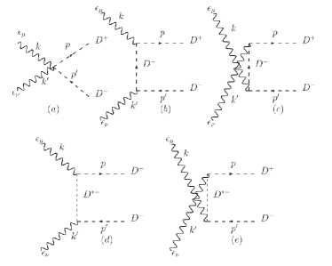
and , and represent the pseudoscalar charm meson (with mass ), the vector charm meson (with mass ) and the photon field, respectively. The Feynman rules can be derived from the interaction terms and they yield the Feynman diagrams for the process shown in Fig. 1a. In the figure we also show the quadrimomenta of the incoming photons , and of the outgoing mesons , . The scattering amplitude can be derived from the Feynman rules.
 |
 |
| (a) | (b) |
As usual, we include form factors, , in the vertices of the amplitudes. We shall follow [12] and use the monopole form factor given by
| (3) |
where is the 4-momentum of the exchanged meson and is a cut-off parameter. This choice has the advantage of yielding automatically and when the exchanged meson is on-shell. The above form is arbitrary but there is hope to improve this ingredient of the calculation using QCD sum rules to calculate the form factor, as done in [13], thereby reducing the uncertainties. Taking the square of the amplitude and the average over the photon polarizations it is straigthforward to calculate the cross section:
| (4) |
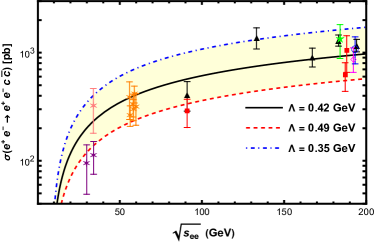
where . We emphasize that the only unknown in our calculation is the cut-off parameter . In what follows, we will determine it fitting our cross section to the LEP data on the process .
From the pair we can construct a bound state (denoted ). As in [4], we impose phase space constraints on the mesons, forcing them to be “close together”. Here we do this through the prescription discussed in [14]. The bound state is defined as
| (5) |
where is the bound state energy, is the relative three momentum between and in the state , are the energies of and and is the bound state wave function in momentum space. From Eq. (5), we can write the following relation between the amplitudes:
| (6) |
We assume that the and hence . Consequently, the relative momentum is close to zero. Therefore the energy and the amplitude depend only weakly on and can be taken out of the integral. Moreover, since the binding energy is small we have and hence
| (7) |
With the amplitude above we calculate the cross section for bound state production:
| (8) |
where is the momentum of the produced bound state and is the flux factor. In the center of mass frame of the collision, we have
| (9) |
where and and are the energies of the colliding photons. The flux factor is then given by . The integrated cross section reads:
| (10) |
where . To complete the calculation we need the wave function of the bound state. In [15] a similar particle made of open charm mesons was studied with the Bethe-Salpeter equation and an expression for the wave function was derived. Here we will just quote the final expression needed to calculate , which is given by:
| (11) |
In the above expressions is the reduced mass (), is a cut-off parameter and is the binding energy. We shall follow [16] and assume that GeV. From [16] we see that one can compute the (dynamically generated) mass of a bound state and then determine its binding energy. Knowing , and fixing , we can use (11) to calculate . In what follows our reference value will be obtained using MeV and the mass of the bound state equal to MeV, as found in [16]. With these numbers we get MeV and GeV3.
The equivalent photon approximation is well known and it is described in several papers [17]. In general, when the photon source is a nucleus one has to use form factors and the calculation becomes somewhat complicated. Here we will follow [18] and define an UPC in momentum space. The momentum distribution of the equivalent photons created by a source with charge is [18]:
| (12) |
where is the photon transverse momentum, its energy and is given by , where is the proton mass. In order to obtain the energy spectrum, one has to integrate this expression over the transverse momentum up to some value . The value of is given by , where is the radius of the projetile. For Pb, fm and hence GeV. After the integration over the photon transverse momentum the photon energy distribution is given by:
| (13) |
Because of the approximations [18] the above distribution is valid when the condition is fullfiled. Using Eq. (13) we can compute the cross sections of free pair production, , and of bound state production, . They are given by:
 |
 |
| (a) | (b) |
In Fig. 1b we show the cross sections for free pair production and compare it to the existing experimental data from LEP [19]. In fact, the LEP data are for , i.e., the measured final states are and . We assume that these two final states have the same cross section and, in order to compare with the data, we multiply our cross section by a factor two. In order to fit these data we will adapt expression (14) to electron-positron collisions. The cross section is the same but the photon flux from the electron (and also from the positron) and the integration limits are different [1, 17, 18]. Comparing our formula with these data, we determine the only parameter in the calculation, which is the cut-off . In the figure, the curves are obtained substituting Eqs. (4) and (13) into (14). In the latter . The band is defined by the choice of two limiting values of . In what follows we will use these values to estimate the uncertainty of our results.
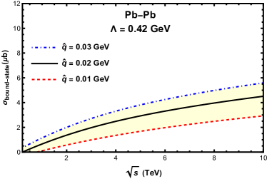
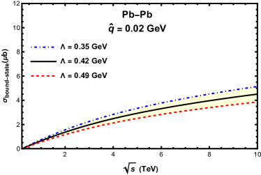
In Fig. 2 shows the cross section for bound state production cross section and its dependence on (Fig. 2a) and on (Fig. 2b). It is encouraging to see that at TeV we have:
| (16) |
This number should be compared with results found in [10] and in [20]. In those papers, the production cross section of scalar states and in UPCs at TeV were calculated and the results were in the range
| (17) |
where stands for or . In both papers the X states were treated as meson molecules, as in the present work. It is reassuring to see that, in spite of the differences, the obtained cross sections are not so different. The cross section (16) should also be compared with the results obtained in [21] for the production of the same state treated as a tetraquark. Interestingly in that work the authors find , more than one order of magnitude smaller than (16). The existence of this significant difference is auspicious for our scientific goal, namely, to use UPCs to discriminate between hadron molecules and tetraquarks. For more information about the material presented in this section we refer the reader to the article [22].
3 Production of very forward pions
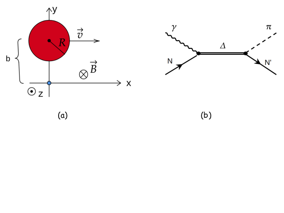
Some time ago, several calculations [23, 24] have shown that in high energy nuclear collisions a very strong magnetic field is produced. Since then, the effects of these fields have been looked for in different physical processes. Perhaps the most famous one is the chiral magnetic effect [25]. Another effect was investigated in [26]. In that work it was argued that in an ultra-peripheral collision magnetic excitation (ME) can lead to pion production. In a ME the projectile creates a field which causes a “splin-flip” in a nucleon in the target, resulting in the process . After the excitation, the decays into pions: . The pions produced in this way have extremely large rapidities. This is in contrast to all other particle production processes in UPC, in which the produced particles have small rapidities. Hence the appearance of very forward pions would be a confirmation of ME and would be a clear manifestation of the magnetic field. In [26] and [27] this process was treated in two different ways.
In what folows we will briefly review the two calculations and compare them.
Let us start considering the collision depicted in Fig. 3a, where the proton is at rest. The incoming nucleus creates a magnetic field which converts the proton into a . As an example, let us focus on the transition . The corresponding amplitude reads [26]:
| (18) |
where , is the mass and is the proton mass. The Hamiltonian reads:
| (19) |
where and are the charge and the mass of the constituent quark of type and is the spin operator acting on the spin state of this quark.
The system of coordinates is shown in Fig. 3a. The field is given by [26]:
| (20) |
where and . The required spin wave functions are:
| (21) |
| (22) |
Now we substitute Eq. (20) into Eq. (19) and the latter into Eq. (18). Then, using the states given above, we calculate the sandwiches of , obtaining the final amplitude. The cross section for the process reads:
| (23) |
For our purpose it is sufficient to have only one proton as target.
In the formalism developed in [27] the cross section of reaction depicted in Fig. 3b reads [1]:
| (24) |
where is given by [1]:
| (25) |
In the above expression is the photon energy, is the radius of nucleus . The Lorentz factor is in the target frame. In the LHC .
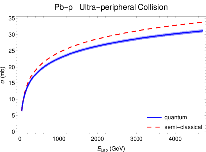
The cross section of the process can be computed from the Feynman graph depicted in Fig. 3b. A simple parametrization of the photoproduction cross section was introduced in [27]. Knowing , we use it to calculate the cross section (24). In Fig. 4 we plot together the obtained quantum (24) (solid lines) and semi-classical (23) (dashed line) cross sections. The band shows the uncertainty related to the decay width [27]. The difference between the results obtained with (23) and with (24) is small and reaches 9 % at the highest energies.
The measurement of these ultra-forward pions may be challenging, but there is some hope. In fact, ultra-forward neutral pions have already been detected in proton-proton and proton-lead collisions at the LHC [28]. Unfortunately, in those measurements it was not possible to focus only on ultra-peripheral collisions. We hope that this could be done in the future.
4 Conclusion
In this work the cross section for the production of a molecule in ultra-peripheral collisions was calculated. It is for TeV. This number is consistent with the results obtained for other scalar exotic charmonium molecules in Ref. [10] and in Ref. [20]. The parameters of the calculation are the hadronic form factor cut-off, the maximum transverse momentum of an emitted photon and the binding energy. All these parameters can be constrained by experimental information and/or by calculations and hence the precision of our calculation can be increased. The method used here can be easily applied to other exotic states.
We have also calculated the cross section for the production of very forward pions. We have used two methods, one with a classical magnetic field and the other with equivalent photons. Both methods yield a similar result: a quite large cross section for forward pion production. The neutral pions can in principle be measured. This would improve our knowledge about the validity of the classical approximation and about the strength of the magnetic field created in these collisions.
Acknowledgments
We are deeply indebted to K. Khemchandani, A. Martinez Torres, A. Szczurek and A. Esposito for instructive discussions. This work was partially financed by the Brazilian funding agencies CNPq, CAPES, FAPESP, FAPERGS and INCT-FNA (process number 464898/2014-5). F.S.N. gratefully acknowledges the support from the Fundação de Amparo à Pesquisa do Estado de São Paulo (FAPESP).
References
References
- [1] C. A. Bertulani, S. R. Klein and J. Nystrand, Ann. Rev. Nucl. Part. Sci. 55, 271 (2005).
- [2] N. Brambilla, S. Eidelman, C. Hanhart, A. Nefediev, C.-P. Shen, C. E. Thomas, A. Vairo, and C.-Z. Yuan, Phys. Rept. 873, 1 (2020); R. M. Albuquerque, J. M. Dias, K. P. Khemchandani, A. Martinez Torres, F. S. Navarra, M. Nielsen and C. M. Zanetti, J. Phys. G 46, 093002 (2019).
- [3] T. W. Wu, Y. W. Pan, M. Z. Liu and L. S. Geng, Sci. Bull. 67, 1735 (2022); [arXiv:2208.00882 [hep-ph]]; D. Marietti, A. Pilloni and U. Tamponi, Phys. Rev. D 106, 094040 (2022). Pioneering studies were presented in S. J. Brodsky and F. S. Navarra, Phys. Lett. B 411, 152 (1997).
- [4] P. Artoisenet and E. Braaten, Phys. Rev. D 83, 014019 (2011); Phys. Rev. D 81, 114018 (2010).
- [5] W. Lucha, D. Melikhov and H. Sazdjian, Phys. Rev. D 100, 014010 (2019); Phys. Rev. D 98, 094011 (2018).
- [6] R. D. Matheus, F. S. Navarra, M. Nielsen and R. Rodrigues da Silva, Phys. Rev. D 76, 056005 (2007).
- [7] A. Esposito, E. G. Ferreiro, A. Pilloni, A. D. Polosa and C. A. Salgado, Eur. Phys. J. C 81, 669 (2021).
- [8] C. Bignamini, B. Grinstein, F. Piccinini, A. D. Polosa and C. Sabelli, Phys. Rev. Lett. 103, 162001 (2009).
- [9] H. Zhang, J. Liao, E. Wang, Q. Wang and H. Xing, Phys. Rev. Lett. 126, 012301 (2021); B. Wu, X. Du, M. Sibila and R. Rapp, Eur. Phys. J. A 57, 122 (2021).
- [10] B. D. Moreira, C. A. Bertulani, V. P. Goncalves and F. S. Navarra, Phys. Rev. D 94, 094024 (2016).
- [11] X. H. Cao, M. L. Du and F. K. Guo, [arXiv:2401.16112 [hep-ph]] and references therein.
- [12] P. Lebiedowicz, O. Nachtmann and A. Szczurek, Phys. Rev. D 98, 014001 (2018).
- [13] M. E. Bracco, M. Chiapparini, F. S. Navarra and M. Nielsen, Prog. Part. Nucl. Phys. 67, 1019 (2012).
- [14] An introduction to quantum field theory, M. Peskin and M. Schroeder, Addison-Wesley (1996).
- [15] D. Gamermann, J. Nieves, E. Oset and E. Ruiz Arriola, Phys. Rev. D 81, 014029 (2010).
- [16] C. W. Xiao and E. Oset, Eur. Phys. J. A 49, 52 (2013).
- [17] G. Baur, K. Hencken, D. Trautmann, S. Sadovsky and Y. Kharlov, Phys. Rept. 364, 359 (2002).
- [18] M. I. Vysotskii and E. Zhemchugov, Phys. Usp. 62, 910 (2019); [arXiv:1806.07238 [hep-ph]].
- [19] W. Da Silva [DELPHI], Nucl. Phys. B Proc. Suppl. 126, 185 (2004); A. Csilling [OPAL], AIP Conf. Proc. 571, 276 (2001). [arXiv:hep-ex/0010060 [hep-ex]].
- [20] R. Fariello, D. Bhandari, C. A. Bertulani and F. S. Navarra, Phys. Rev. C 108, 044901 (2023).
- [21] A. Esposito, C. A. Manzari, A. Pilloni and A. D. Polosa, Phys. Rev. D 104, 114029 (2021).
- [22] F. C. Sobrinho, L. M. Abreu, C. A. Bertulani and F. S. Navarra, arXiv:2405.02645 [hep-ph].
- [23] V. Skokov, A. Y. Illarionov and V. Toneev, Int. J. Mod. Phys. A 24, 5925 (2009).
- [24] V. Voronyuk et al., Phys. Rev. C 83, 054911 (2011); C. S. Machado, F. S. Navarra, E. G. de Oliveira, J. Noronha and M. Strickland, Phys. Rev. D 88, 034009 (2013).
- [25] For a recent review see: D. E. Kharzeev, J. Liao and P. Tribedy, arXiv:2405.05427 [nucl-th]].
- [26] I. Danhoni and F. S. Navarra, Phys. Lett. B 805, 135463 (2020).
- [27] I. Danhoni and F. S. Navarra, Phys. Rev. C 103, 024902 (2021).
- [28] O. Adriani et al., LHCf Collaboration, Phys. Rev. D 94, 032007 (2016).