[1]\fnmTsung-Wei \surHu
[1]\orgdivDepartment of Mathematics, \orgnameUniversity of Georgia, \orgaddress\streetHerty Drive, \cityAthens, \postcode30602, \stateGeorgia, \countryU.S.A
2]\orgdivDepartment of Mathematics, \orgnameUniversity of Georgia, \orgaddress\streetHerty Drive, \cityAthens, \postcode30602, \stateGeorgia, \countryU.S.A
A Construction of Interpolating Space Curves with Any Degree of Geometric Continuity
Abstract
This paper outlines a methodology for constructing a geometrically smooth interpolatory curve in applicable to oriented and flattenable points with . The construction involves four essential components: local functions, blending functions, redistributing functions, and gluing functions. The resulting curve possesses favorable attributes, including geometric smoothness, locality, the absence of cusps, and no self-intersection. Moreover, the algorithm is adaptable to various scenarios, such as preserving convexity, interpolating sharp corners, and ensuring sphere preservation. The paper substantiates the efficacy of the proposed method through the presentation of numerous numerical examples, offering a practical demonstration of its capabilities.
keywords:
Spline, interpolation, Smooth curve, CAGD1 Introduction
Curves are fundamental geometric objects with applications in various fields that require different types of curve construction and design. The study of constructing smooth interpolatory space curves has been ongoing for many decades. In this paper, we are interested in constructing space curves in with , aiming to satisfy the following requirements:
-
•
interpolation, that is, the curve passes the given designed points;
-
•
smoothness, that the curve must be geometrically smooth with , We shall present our construction of curves in this paper.
-
•
locality, i.e., any local change of the given points only affects the curve locally.
-
•
no cusp points and no self-intersection unless there is such a need;
-
•
convexity control capability;
-
•
conic preservation, i.e. if a part of the given data points is from a sphere, the curve passing these points is also on the sphere.
-
•
invariant under the translation and rotation of the data points;
-
•
corner points are also possible. In particular, the sharpness of the corner points is controllable.
Many approaches are available in the literature and practice to construct smooth space curves due to the active study in the last several decades. However, constructive methods satisfying all the above requirements are few, The requirement of the high order smoothness, say is one of the main hurdles for interpolating curve construction. The high-order smoothness needs a lot of more parameters than the construction of curves and hence the parameters are hard to control while easy to produce the cusps and/or overshoots in the curve. It is well-known that the smoothness of the parametric functions for a curve does not ensure the smoothness of the graph of the curve or a geometrically continuous curve. An example will be presented in Example 2.1. Typically, the distinction between the ”smoothness of graph” and ”smoothness of function” is made using the concept of geometric continuity (cf. [1] [2] [3]). In this paper, we define the geometric continuity of a curve by considering the regularity of its parametric functions. Please refer to Section 2.3 for the formal definition.
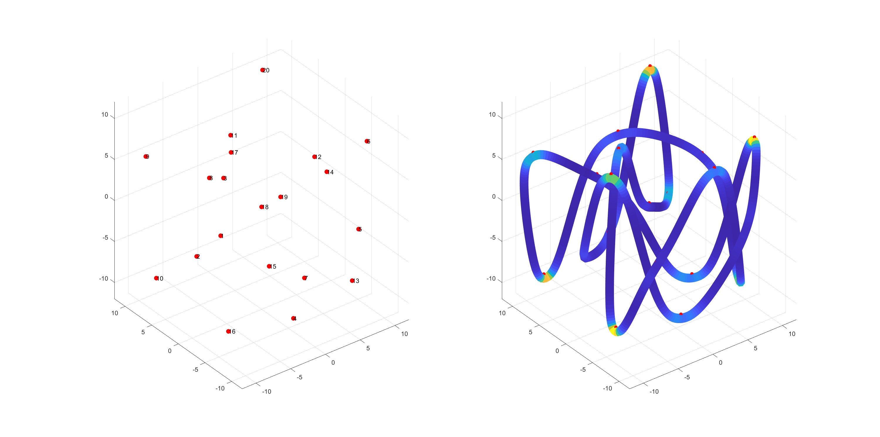
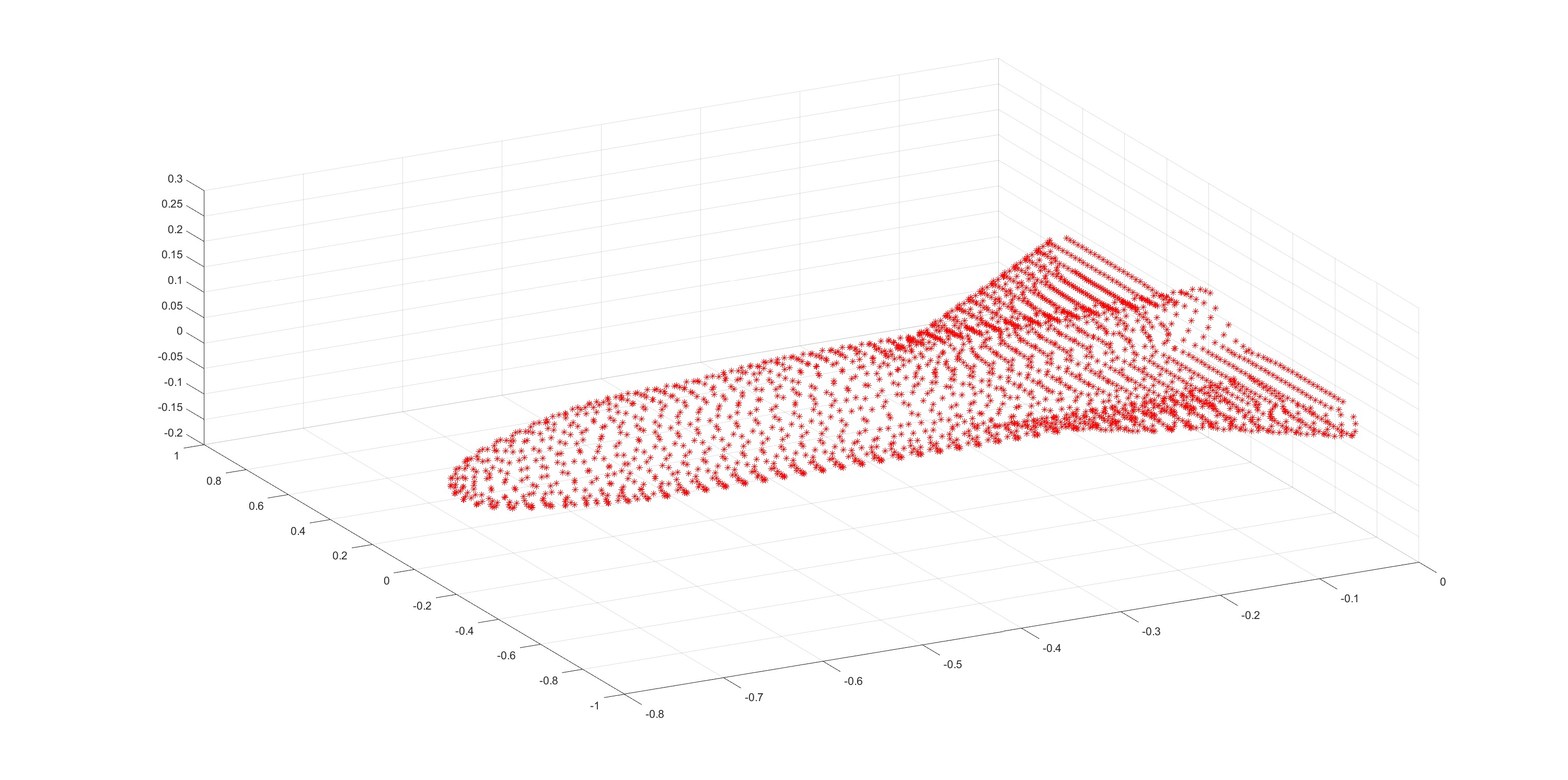
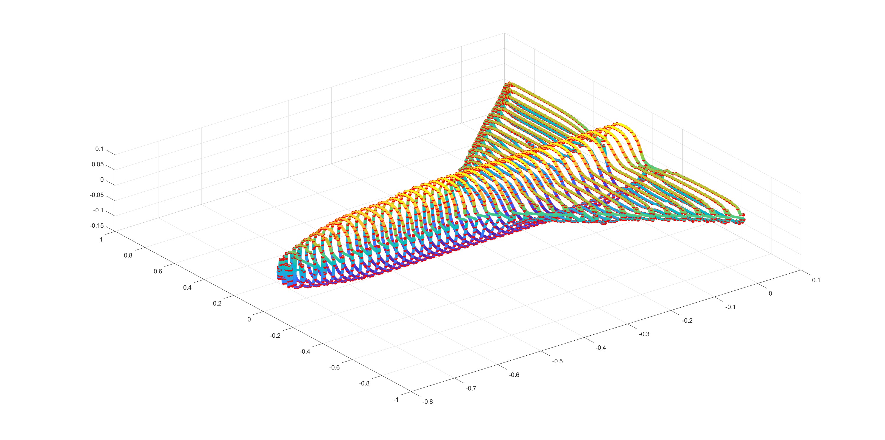
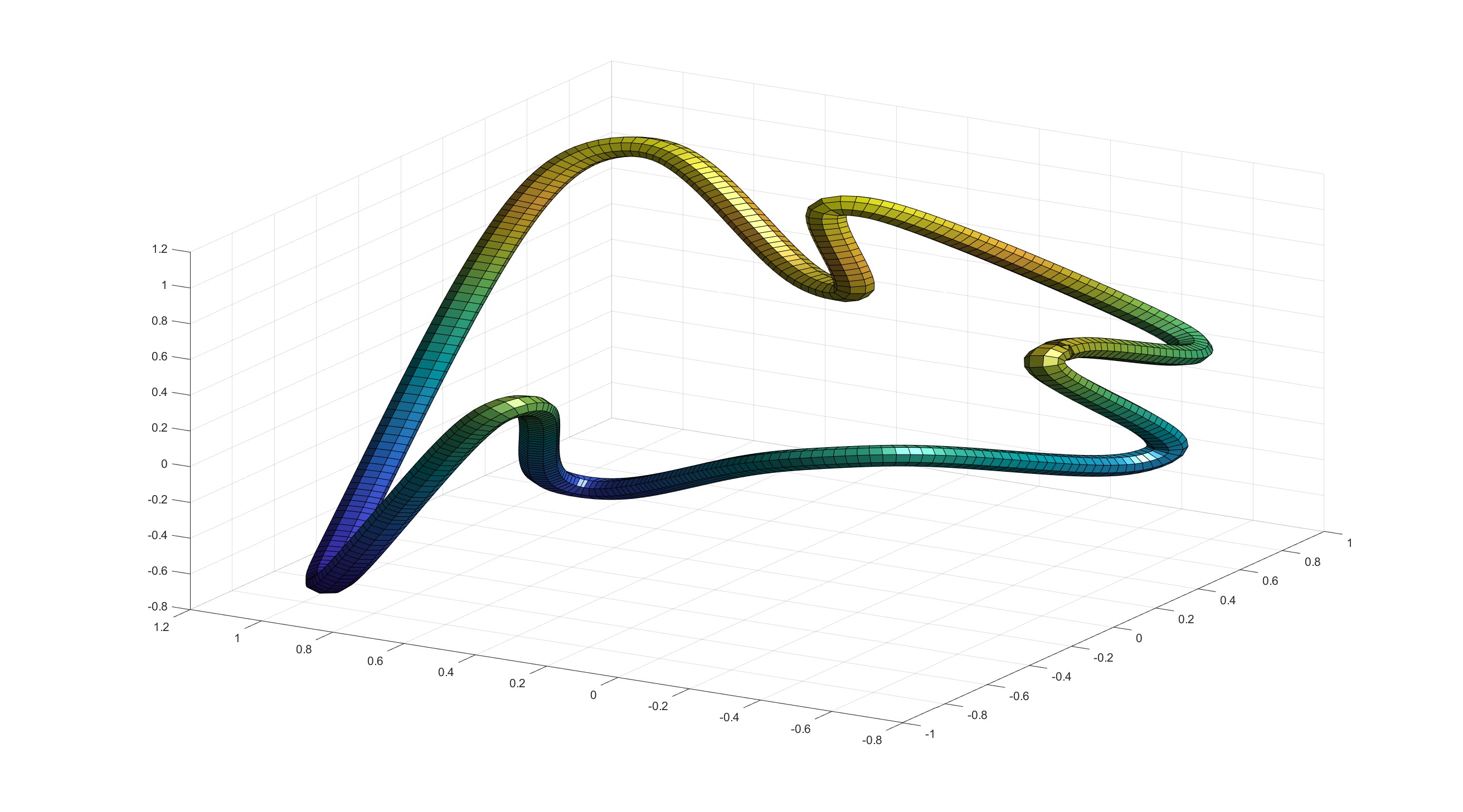
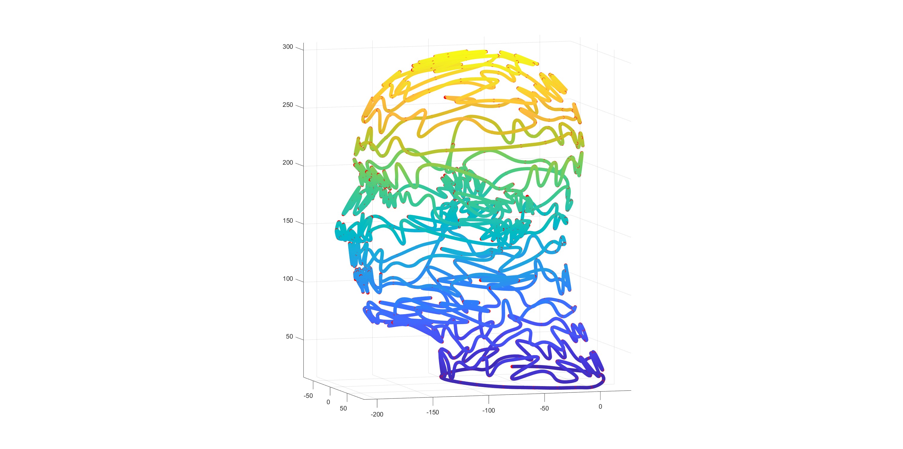
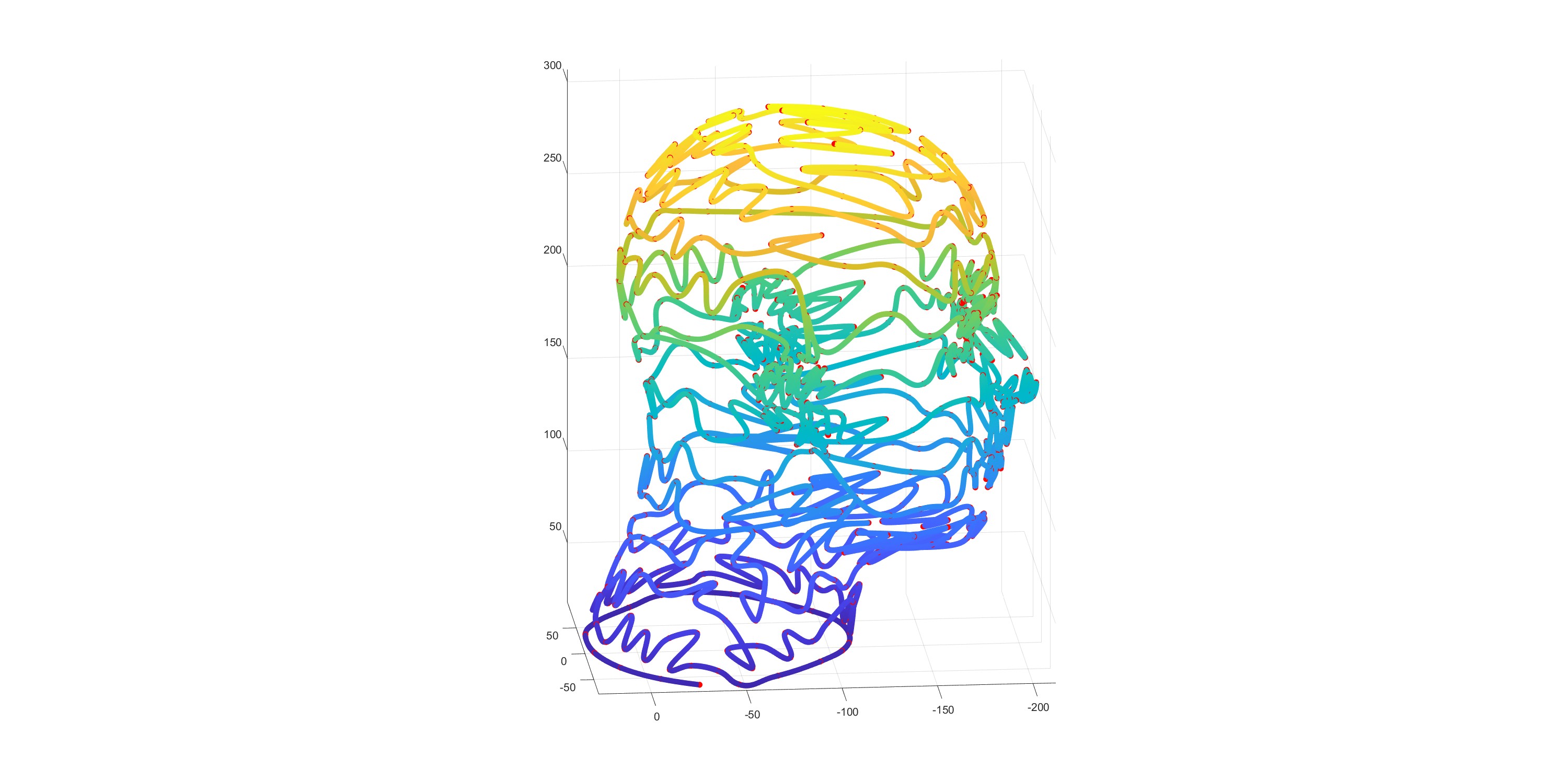
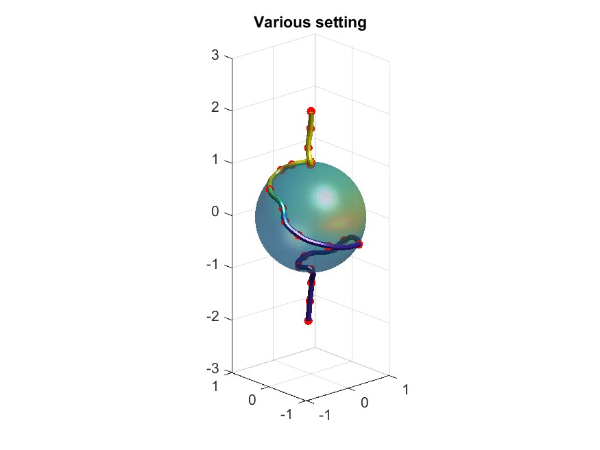
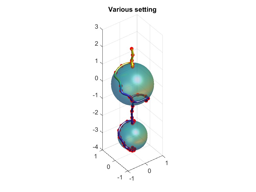
Let us first present two examples of curves based on our construction in Figure 1 and Figure 2. We give sets data set in which are oriented data sets, and the data sets are flattenable to be explained in Definition 2.1. These figures show that our construction works nicely for various sizes of data points. In Figure 1, we have 20 points while in Figure 2, we have 2776 space points. More examples will be given in a later section to demonstrate that our construction can preserve the corners, preserve circle or sphere when the data points are on a circle or on a sphere.
Our method of construction shares similar steps with previous methods in the literature. More precisely, our algorithm can be decomposed into four parts: local curve construction, redistribution, blending function construction, and gluing two pieces together. Let us quickly outline each of the four components as follows.
-
•
Local Curves Consider the series of points , we define a local curve be a the curve pass , where for . There are few canonical options for local curves: parabola, circle, or Bézier curves. We shall explain them in much more detail in Section 3.1.
-
•
Redistribution Once we have a local curve (function) , the reparametrization of the function will not change the graph. Therefore, we can reparametrize the curve in a conventional way. One of the convenience ways is let where for , and is linear on and . We define . Note that is piecewise linear, so is only , but since it parametrizes the same curve as , so is still has a smooth graph.
-
•
Blending Function For short, a blending function is a pair of functions with , , and for all . One can understand it by weighted functions of endpoints and . We shall impose an additional assumptions on the derivative in need for the smoothness, see details in Section 3.3.
-
•
Gluing Two Pieces Together After redistribution, and have over lapping domain . We can define a new function
More generally, if we have a continuous function with and , we can gluing the function as
This is particularly useful if we know some extra features of the original data. For instance, in the section on numerical experimental results, we will have two examples to show when the point data are on the sphere, we can make sure our interpolating curve is on the same sphere as well by choosing a suitable .
1.1 Related works
The realm of curve construction is vast, and a complete overview is not within the scope of this paper. Here, we present a selection of essential works that are more related to our work. Farin [4] provides a thorough organization of curve interpolation methods using -splines in his book. He also discusses Bézier curves, a group of smooth curves based on polynomials. Two primary challenges associated with Bézier curves are the need for a local shape control algorithm adaptable to various cases and the difficulty in achieving a higher order of continuity due to the flexibility in choosing control points.
To achieve a local shape control, various methods are employed to interpolate curves. One example is the Non-uniform Rational B-spline (NURB) [5], which utilizes a rational polynomial as a substitute for the conventional polynomial. This substitution provides a broader range of shape options with a reduced number of control points. Addressing the specific need for circle interpolation, a blending technique of the circular functions was introduced [6]. Notably, Yuksel [7] made significant advancements by replacing the local circular function with an ellipse function when the given data points deviate from a circle. Another noteworthy approach involves the use of clothoids to interpolate curves, offering a method for achieving curves with uniform curvature changes [8]. While these algorithms enhance curve fitting in diverse scenarios, it’s important to note that they may introduce increased curve complexity, and the highest achievable smoothness of these algorithms are limited to .
Some approaches center around polynomials and aims to enhance smoothness. One approach is to interpolate the curve independently along different axes. Let , one can interpolate , , and by , , and , where for . Further details are expounded in the book by Knott [9]. Subsequent to this, Lee refined the selection of [10] and made the curve more appealing. Key challenges associated with interpolating along different axes include the absence of locality and a deficiency in rotational stability.
Our algorithm is grounded in the notion of blending functions. By introducing the -blending function, one can craft an interpolation function with a desired shape and achieve any desired level of smoothness. We redefine geometric continuity in an alternative manner and provide a robust methodology for generating curves without cusps or self-intersections.
1.2 Organization of the paper
The paper is organized as follows. We will explain the concept of the oriented data point set and points that are flattenable. Then, we explain the concept of geometric continuity and the geometrical smoothness of the graph of a curve. These will be done in Section 2. we explain our constructive steps with emphasis on the four components that we explained in the introduction. We will give a very general definition of these components and provide a detailed justification of how smooth these curves are. We also use the ideas to create a few new categories of curves that achieve any given smoothness while consisting of piecewise polynomials or preserving the shape of a circle and/or sphere.
2 Preliminaries
In this section, we first explain the concepts of oriented point sets and flattenable point sets. Then, we explain the regularity of a graph and geometric continuity/smoothness.
2.1 Oriented Set of Points and Flattenable Points
Consider the set of space points in which is oriented in the sense that is connected to for all in the setting of space curves. We call it sometimes a 1D-oriented point set, sometimes an oriented curve data set, or sometimes a curve data set, just for simplicity. Next, we introduce the concept of flattenable points.
Definition 2.1.
An 1D-oriented point set is said to be flattenable if for any three consecutive points there exist a line in such that the projections of these three points to preserve the order of these three points, i.e. the projection of is in the middle of the projections of and .
2.2 Regularity of the Graph of Curves
Consider a curve consisting of points in which are defined by one variable parametric functions. For instance, a non-self intersects curve in can be defined by , where for an interval and are coordinate functions of , where . We call a parametrization function of the arc, and the arc which it parameterized is called the graph of . Obviously, if is continuous, then its graph is continuous. However, the parametrization functions’ smoothness is insufficient for the graph to be smooth. Let us look at the following example.
Example 2.1.
Let for . The parametric functions are differentiable, but the graph of is not. As shown in Figure 3, the curve has a cusp at . That is, the smoothness of the parametric functions did not guarantee that the graph of the parametric curve looks smooth.
In the Example 2.1, the cusp happens at where the tangent vector vanishes. Indeed, if the graph looks smooth, it should at least have a continuous tangent. However, the of its parametric function does not imply this property as we saw in the Example 2.1. To distinguish the ideas, we call a graph of a parametric function has a geometric continuity of degree 1 (denoted as ) if it has tangent lines on each point on it. If we think about the sufficient condition for a parametric function to have a graph, we use the following definition:
Definition 2.2.
A parametrization function is said to be regular at if .
The vanish of the first derivative of gives us the graph without continuous tangent. We can easily see the following property is true.
Proposition 2.2.
If a pasteurization function is regular, then its graph is .
We may now extend the ideas to the high order of geometric smoothness. In addition, if is continuously differentiable in parameter , its curvature which can be formulated as [11]:
| (1) |
Since , the curvature is well defined. If the curvature is continuous, we can say that the graph of parametric curve has continuous tangent and curvature. In general, the non-vanish of the first derivative is sufficient for a curve that has geometric continuity up to order .
To summarize, the regularity of the parameterization makes the graph have geometric continuity up to the smoothness of the parameterization. We remark that:
Remark 2.1.
A regular curve has continuous tangents on its graph. A regular curve has continuous curvatures of its graph.
In the end of this subsection, let us present an example that a linear combination of two regular curve pieces may not be regular any more.
Example 2.3.
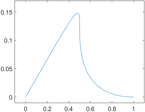
Let , and 1-blending function with . and are regular curve with
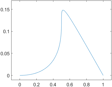
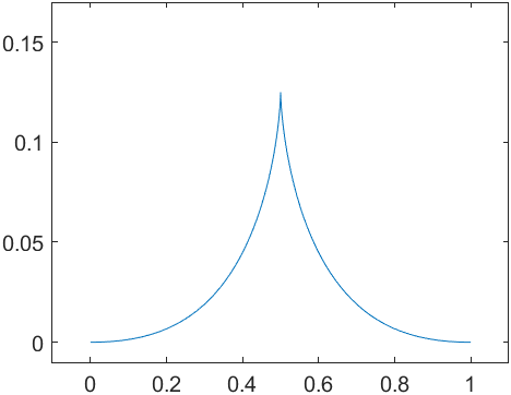
which connect two points and for . However, the weighted sum is not regular and not at . See the graph on the right of Figure 5.
2.3 Connection of Geometric Continuity Curves
For curves, the regularity of its parametric function can guarantee nice-looking graphs. However, in most practical applications, joining multiple curves with different parametric functions is required to express a long curve. That is, we may not have a global regular parametric function for the entire curve. It is possible that we may still have a nice-looking entire curve even if the parametric functions of each piece are not joined smoothly. Let us see the following example.
Example 2.4.
Consider a parametric curve defined below.
The graph of is a line segment from to in which joins smoothly at . However, the parametric function itself is not differentiable at . Nevertheless, we can define a bijection , where
such that for . We can see that is now a regular parametric function even though and are not smooth at .
We see the existence of a regular parametric function is crucial to the geometrical smooth feature. We are now ready to formally define smoothness for for a curve consisting of multiple pieces.
Definition 2.3.
[cf. [12]] Fix . A graph of curve in is said to be continuity at a point if there exist a regular parametrization of functions and a constant such that with and is a nonzero vector, i.e. . An entire curve in is said to be continuous if the curve is of continuity at each point on the curve.
In short, the continuity is a property of a curve-like subset in . Regularity and are properties of the underlying parametric functions of the curve. Figure 6 shows the idea of the Definition 2.3. Let us summarize the above discussion in the following remark.
Remark 2.2.
-
•
A curve with parametric function does not imply the graph of the curve is . See Example 2.1.
-
•
If a curve with parametric function is regular, the graph of the curve is .
-
•
The graph is of does not imply its parametric function is regular or . See Example 2.4. However, if is a continuous function, for any , there exist a bijection function , which defined on small interval with , such that is regular and on .
In other words, a bad graph (not ) may have a smooth parametric function, but it can not have a regular smooth function. Vice versa, a graph could adapt different parametric functions and , see Example 2.4. Figure 7 shows the relation between the function and graph. It’s unnecessary to describe a smooth curve with a smooth parametric function. However, there must exist one regular function which parametrizes the curve.
3 Construction of Geometric Smooth Interpolatory Curves
This section is divided into five subsections. In the first four subsection, we explain our construction. We shall suppose that a point cloud in is oriented and is flattenable. We start the construction with the local curves, reparametrizing them (i.e. redistribution), constructing a blending function, and gluing them together. In addition to these four subsections, we shall show that the regularity of the curves based on our construction in the fifth subsection.
3.1 Construction of Local Curves
Given 3 ordered point in , we want to construct a regular curve interpolating these three points.
Definition 3.1.
A function is said to be a local interpolating function of (at point ) if is regular function and there exist a point such that .
Note that we do not require or during our construction and we will still get an interpolating curve after gluing them together. However, having local curves pass and gives us more pleasing curves in most cases. Let us construct a few different types of local interpolating curves in the following examples.
Example 3.1 (Spatial Parabola).
Suppose are three successive points in a flattenable data set. We define and are two vectors which is an plane that contains . Since is flatenable, one may choose such that the projections of to the -axis preserve the order, says . Moreover, we can interpolate by , where is a quadratic function satisfying by choosing and carefully, see Figure 8. The proof of the existence of such construction is left to the reader.
To obtain a parametric function from the above construction, we need a rotation. Let us use for as the coordinate in , as the example. We rewrite , . We can then define , i.e.
We can see that is regular by
which is never zero. Hence, the parabola is a local interpolating function.
The various can be visualized in Figure 9.
Example 3.2 (Arc of Circle or Ellipse).
It it known that 3 points in can uniquely determine a circle (a line can be seen as a degenerated circle) so are the points in when they are flattenable for . If are flattenable, we can choose an arc of the circle in which is located within the arc while and are the endpoints of the arc, see the left of Figure 10. However, the circle arc could be very off when the angle is relatively small (Middle of Figure 10). In [7], Yuksel proposes to use the ellipse arc instead if one of the arc , has corresponding to an angle larger than 90 degrees. The construction can be described as follows: first, place on one axis of the ellipse. Second, place either or on another axis of the ellipse, depending on which further from . Then, there is a unique ellipse that passes through three points with the axis with the specified property. See the right of Figure 10.
The parametric function of the arc can be defined by the polar coordinate. As shown in Figure 11, We can parameterize the arc by , where and axis of circle or ellipse. One can easily see that the parametric function is a regular local function.
Remark 3.1.
If the curve has endpoints, then we need a local curve that passes through (and ). One natural choice is the line segment connecting and ( and ). Or, if our local curve of also passes , we can use the same local curve as . If the curve is a closed circle, say , we have to get another local curve at , which may be a parabola pass , , and or other local curves depend on needs.
3.2 Redistribution and Quasi-regular Local Curves
Suppose is a local curve at , where , , and . Redistribution of is a re-parameterization of the function by using , where the bijection with , , and . We call quasi-regular function (QR function). The formal definition of the quasi-regular local parametric function can be described below:
Definition 3.2.
A function is said to be a local quasi-regular interpolating function of (at point ) if:
-
•
and are regular and .
-
•
for , and for .
-
•
There exists a local re-parameterization with such that is a regular function on for a .
By condition 1) and 2) in Definition 3.2, we can see that is on . By condition 3), we can see that is at . Hence, is on . This is not a surprise if we see that is just the re-parametrize of . The main problem is to choose the distribution function . We see that using a piece-wise linear function will work.
Lemma 3.3.
For a local curve which interpolate , and . Suppose is a piecewise linear function consisting of two line segments such that and . Then is a quasi-regular parametric function such that for .
Proof.
First, is a linear function on . We have
.
Hence, is a regular curve on because
is a constant and
is regular (so that is never zero). Similarly, is a regular curve on .
Secondly, one can easily see that exists when .
Finally, it easy to see that and is a regular function. Thus, is a quasi-regular parametric function.
The interpolation property could be obtained by , , and .
Since and only differ in the parameterization, they have the same graph, which is . Although loses its regularity at the nodes, it stores the point cloud at integer nodes, which is a more desirable property in computer programming.
Before we move on to constrict some local curves, we shall define another important property of these quasi-regular functions.
Definition 3.3.
We say a local interpolating QR function , as we defined in Definition 3.2, is contracted if the inner products
and
where is the piecewise linear function with , , and
We illustrated the contracted local curve in Figure 12. Generally speaking, a parametric function is contracted if it is always closer to than the linear interpolating on both sides.
Another important property is the positive definiteness:
Definition 3.4.
We say a local regular (which also imply ) function on an interval if for all .
Generally speaking, if a curve is positive definite, then it’s target is always toward the endpoint.
The contractness and the positive definite are sufficient conditions of the final gluing curve to be . Hence, we shall prove our construction of local curves are contracting and positive definite.
Example 3.4 (Contractness and Positive definite of Spatial Parabola).
Let , where is defined as in Example 3.1, and is join of two linear functions with , , and . We can prove that is a positive definite curve and contracted at , is a positive definite curve and contracted at .
For positive definiteness, we check the graph on as in Example 3.1, where the parabola curve can be described as on the coordinate systems with origin at . Since is the vertex of the parabola, all the derivative is toward the vertex, i.e. . For , we have
Note that is a linear incresing function on so is a positive constant. Similarly .
For contractness (cf. Definition 3.3), let , since is a linear function from to and is a linear function, we have , where is a linear function with and . Now let we can calculate . Because if is convex, and and if is concave, and . Similarly, for .
3.3 Blending Functions
We begin with a construction of blending functions.
Definition 3.5.
A pair of r-blending polynomials is a polynomial satisfying the following:
-
•
, on .
-
•
and .
-
•
for all .
-
•
on .
-
•
and are non decreasing.
An example of a 0-blending function is
| (2) |
An example of a 1-blending function is
| (3) |
Another example of a 1-blending function is
| (4) |
We can also generate -blending function. let , we define
| (5) |
is not hard to find that satisfying Definition 3.5. Principally, this will give you a interpolation function if you use these in Algorithm 1. However, the derivatives of those blending functions are complex, which may not be suitable for computational manner.
In general, we can generate -blending functions by polynomials , , where . This is equivalent to and , where are -th Bernstein basis polynomials of degree . We call this polynomial r-blending function. There are still many ways to define r-lending functions. We leave them to the interested reader.
3.4 Linear Gluing of QR Curves and Main Theorem
Consider are QR interpolating functions of the data points . Our final glued function to be:
for . Note that and are boundaries QR function. See Remark 3.1. We will show that can be if we carefully choose our , , , and . Indeed, we have:
Theorem 3.5.
Suppose a set of oriented data point . We define a curve
where:
-
1) are local curve which for some for . is a function with , and is a function with .
-
2) is positive definite and contracted to , where piecewise linear function with , , and . When , are linear function where , , , and .
-
3) , are -blending function.
Then the graph of is which .
We divided the proof into three claims:
Claim 3.6.
The defines in Theorem 3.5 interpolate the data points .
Proof. The simple substitution .
Claim 3.7.
The graph of is at integer points.
Proof. Consider for . We want to show that is at . We can consider a re-parameterization . We can show , for , by calculate:
For the second and third term, Note that are a linear function to , so has range on when . We have for and for , since and are -blending function and . This leads to the conclusion that the second term is vanish. For the third term, we know the derivative of is zeros but we need to check if is exist and finite. Note that is a linear function from to . We can conclude that is exist and finite. Hence, the second and third terms all vanish and
Similar to the left-hand limit, we have for . Therefore, is regular function (so ) near . is near because it and have same graph.
Claim 3.8.
The graph of is on intervals for .
Proof.
By definition of , is not hard to see that is a function on . For , we only need to show that is regular, that is, .
We can calculate:
| (6) | ||||
Note that in the last line, we use . Now consider the inner product . We have and because and are positive definite function. For the last component in 6, we consider be a linear function with and . We can calculate
Where we apply the contractness of at and at in the last line. We have is a positive definite on , so it is regular because the first derivative never vanishes.
Corollary 3.8.1 (Bonus Smoothness).
If the local function in Theorem 3.5 is and pass three point , , and , and the -blending function are differentiable up to (The derivative still vanish up to ). Then the curve is .
Proof. We already show the curve is regular. We only need to show that the -th derivative is equal to the Local QR function on its boundary. From Equation 6, we have
| (7) | ||||
When , the first term equal to because and the rest terms of , goes to zeros. For the second term, although is not zeros, . Hence when . Similarly, for .
4 Numerical Examples of 3D Smooth Curves
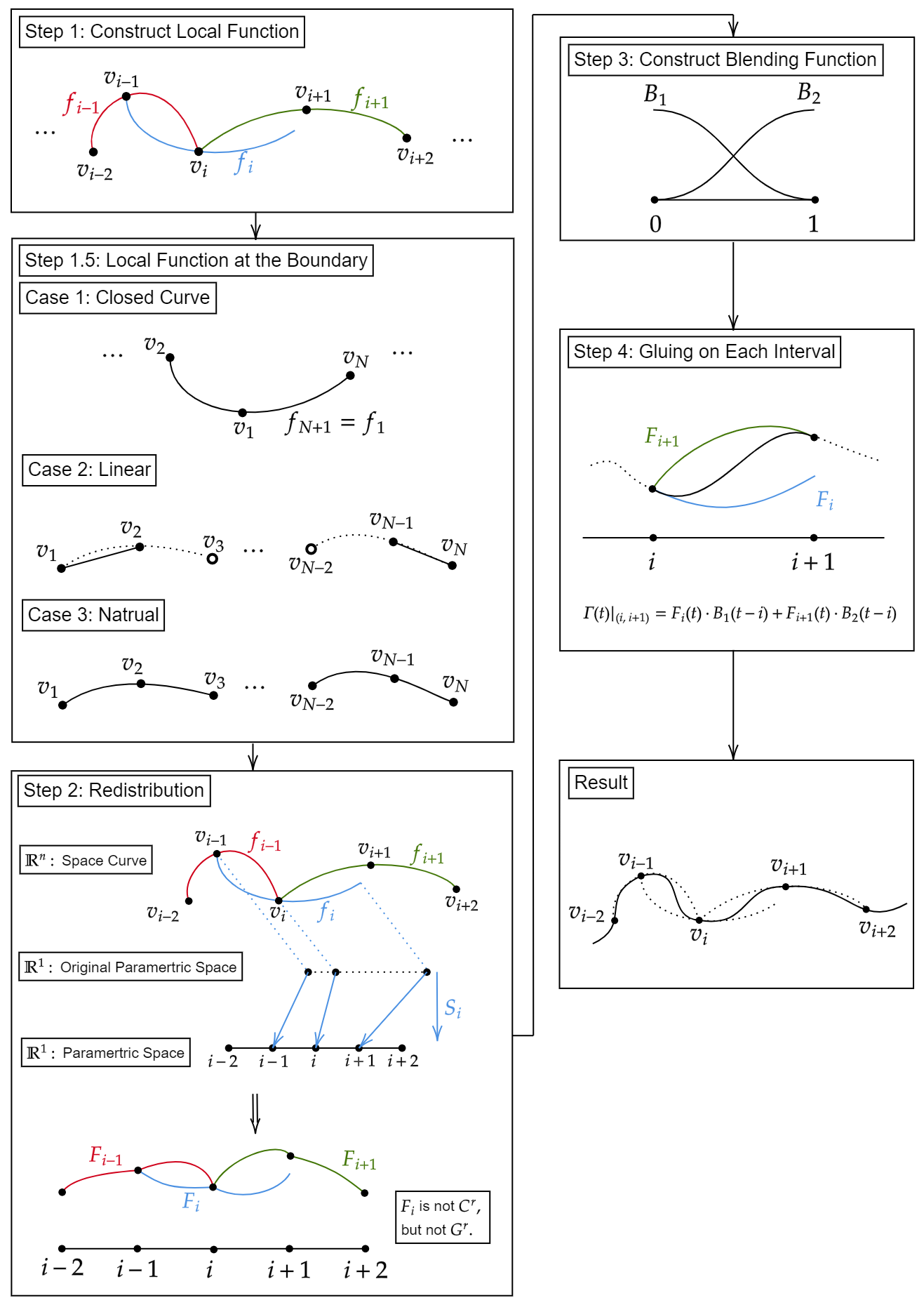
In this section, we present several examples to demonstrate that the method discussed in the previous section can be used to construct smooth 3D curves. We begin with our computational algorithm below, which has been implemented in MATLAB.
Step 1 For each point , use and to generate as in Definition 3.1 for .
Step 1.5 For boundary point and , constructing the local curve and . Some canonical choices are:
Linear Using linear function connect and , and connect and .
Natural If local function pass and , simply use them as the and .
Close If , means the data points is a close curve, we can define be the local function using ,, and .
Step 2 Redistribution the local function .
Step 3 Given smoothness , choose a suitable blending function , .
Step 4 For each interval , evaluate the function .
In addition, we present a computational flowchart to illustrate the steps of Algorithm 1 in Figure 13.
4.1 Computational Experiments
Let us show some numerical results based on our Algorithm 1 above.
Example 4.1 ( Spline Interpolating Curves).
Fix .
We start with the interpolation with piecewise polynomial construction.
We use the parabolic local function from Example 3.1. We already proved that the local QR function is positive definite and contracted in Example 3.4. Therefore, by theorem 3.5 and Corollary 3.8.1, the interpolation is , where is only depending on the choice of -blending function. We use the polynomial -blending function defined in Section 3.3. The degree of -blending function is . In this case, we can construct interpolation spline with piecewise polynomials of degree . In the case , we use degree polynomial to interpolate data in any dimension. This result is quite comparable to Bernstein interpolation. Our algorithm automating the local curve so the user does not have to specify the local control points. In addition, our algorithm can increase the smoothness at a very low extra cost. Because the local curve is the same we only have to compute the blending function which the explicit formula of the function was given.
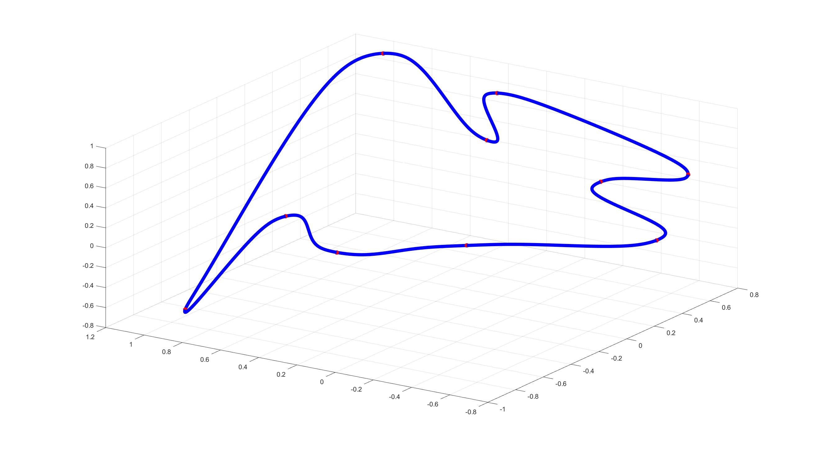
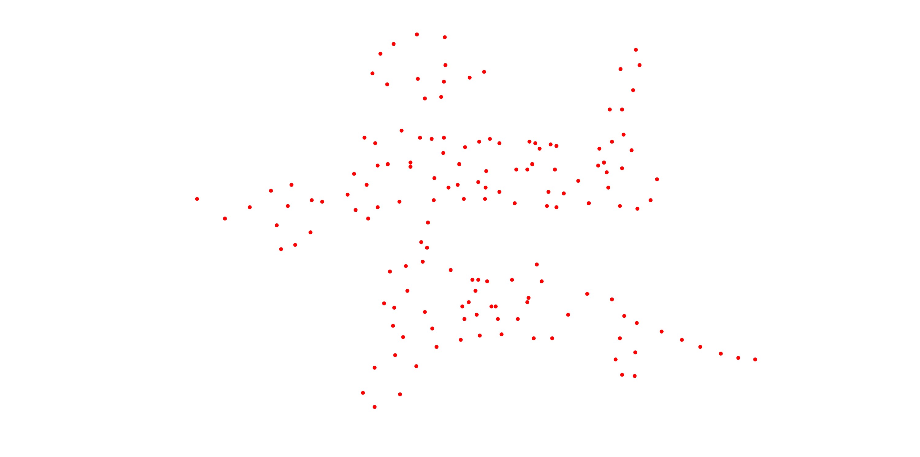
For a set of random points in 3d space, we use -blending function to have smooth curve interpolation. As shown in Figure 14, every point in the original data set (red) is passed by the curve. On the other hand, We can calculate the curvature of the curve to show that the curve can achieve at least , see Figure 1 for the color pattern for the curvature. To show the smoothness of the spline interpolatory curve, another example is given in Figure 14 in tube view.
As we can see in Figure 1, the curvature is higher near data points, which is a desired feature. Some other methods like Circular spline will have curvature peaks in the middle between data points.
 |
 |
 |
 |
Example 4.2 (Corner Preservation).
On planar data points, the data points themselves are not always suitable for smooth interpolation. See Figure 17. In the Figure, we see that in order to interpolate the point at the corner, we must have a curve that is not a straight line. To address this feature, we have the following definition:
Definition 4.1 (Lacol Convex and Degenerate Points).
Consider a series of data points on , we say point is a local convex point if , , and are non-zeros and have same sign. We say 3 is degenerated if at least one of these three determination are zero.
We can illustrate the local convex points in the Figure 18. In the figure, let ray start from with direction , and ray start from with direction . We can get a region by these two rays and line (See shading region in Figure 18). One can easily check that if is located in the slash region, then is a local convex point. If is on the boundary of the slash region, then it’s degenerated. One important case of degenerate points is when is at the intersection of and . The smooth interpolation curve will not be pleasing. We say is a corner in this case. In Figure 17, the red points are corner points. We see that the interpolation curves lose local convexity when the original polygon is local convex. In practice, we can easily detect corner points and replace the local function to be piecewise linear.
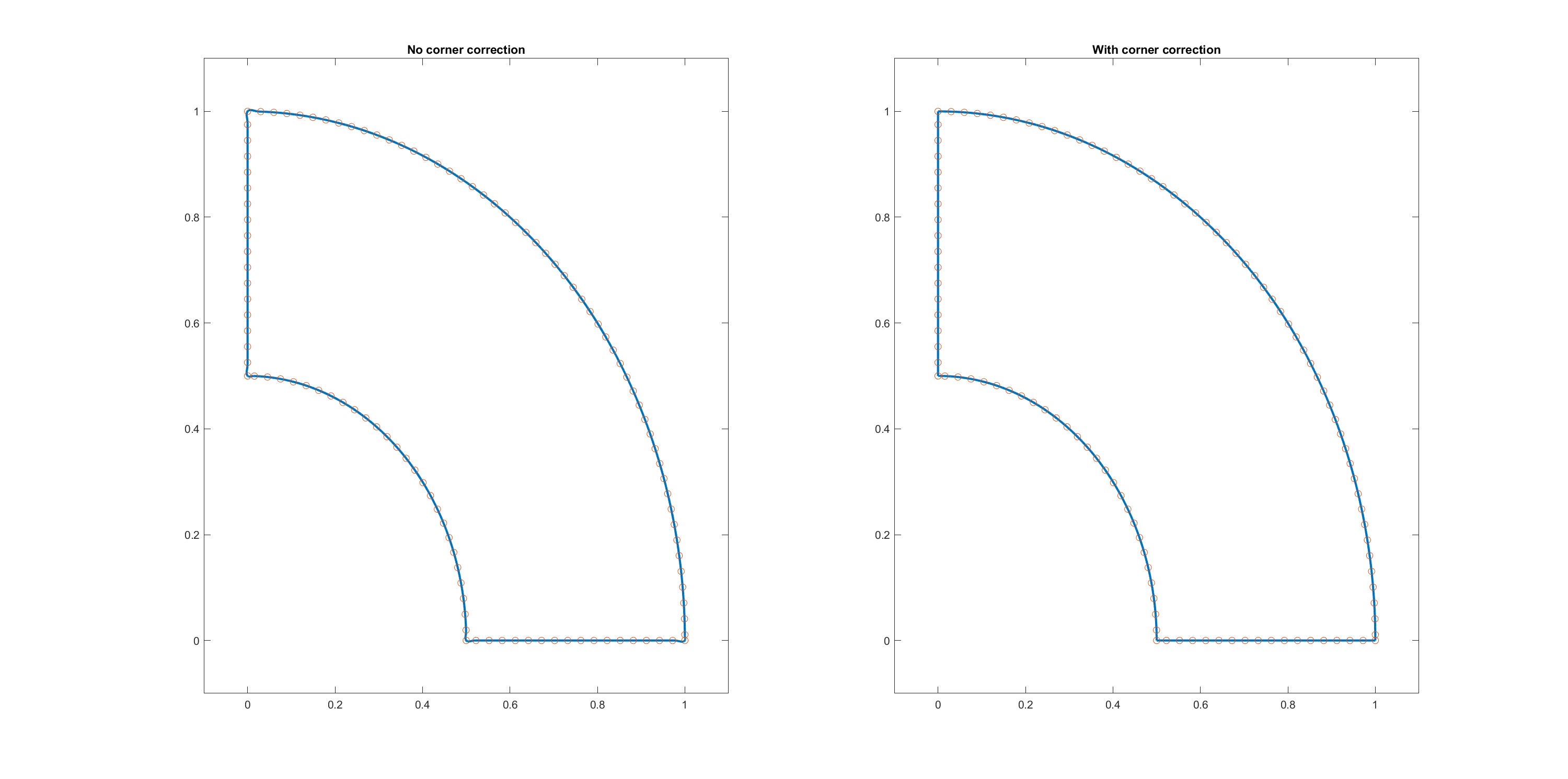
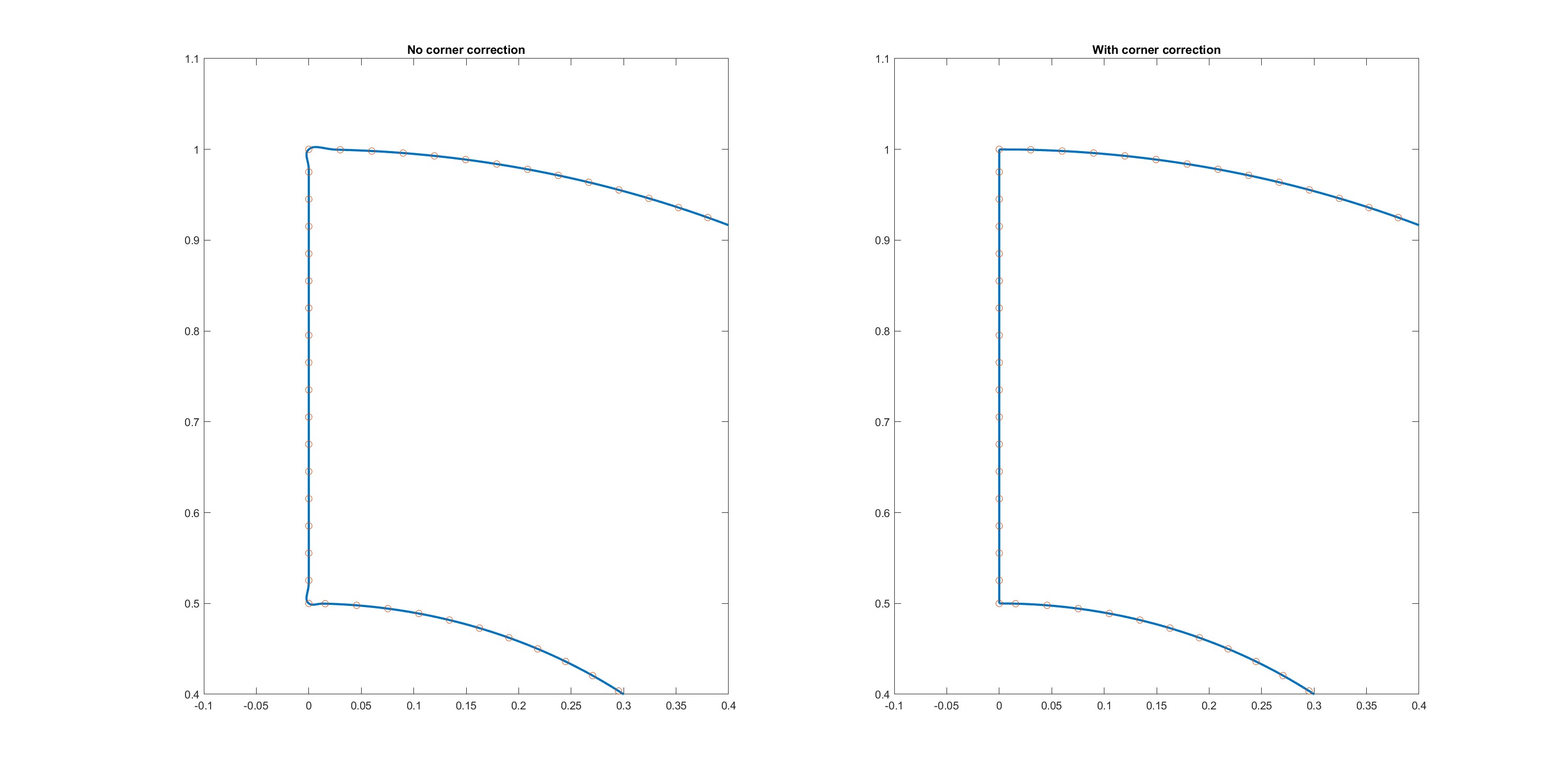
We show an example of taking care of the corners of a given data set. Suppose that we have a set of data with four corners. If we use our method straightforwardly, our smooth interpolating curve will have rounded corners. See the left of Figure 19. When the code recognizes a point as a corner, it skips the local constructive step and produces the curve with corners by replacing the local curve with a piecewise linear function, as shown on the right of Figure 19.
Example 4.3 (Convex Planar Data).
We defined local convex points in Definition 4.1. A natural question arises here: could we preserve the local convexity? That is, if is a local convex point, could we have such that do not change sign on its curvature? The answer is affirmative. We can achieve this by choosing a linear local curve. Indeed,
let be a series of points and , , and are local convex points. Suppose tangent line , are ordered clock-wisely as show in Figure 20. Then there must be a line pass through which one of its direction vectors is located between and , shown as the blue line in Figure 20. Because and are also local convex, we can find two similar lines pass and , shown as orange lines in Figure 20. The and are intersections of the blue line and orange lines. The linear function from to is defined as the local function in this example.
We claim that if we use these local functions and the polynomial -blending function, then the resulting curve is local convex as long as the data points are local convex. The proof is quite straightforward. We already claim that the -bending function is equivalent to Bernstein polynomials:
| (8) |
Back to our example in Figure 20. We shall show that the line segment from to is local convex. We know that on , and . Combine with the formula of blending curve, one can write down the curve by Bezier polynomial:
where are -th Bezier base polynomial of degree . As we can see, this line segment is a Bezier curve where all control points are located on the - and -. The control points form a convex polygon. By variation diminishing property, the curve is a local convex curve.
Example 4.4 (Sphere Preserving Curves).
In this subsection, we present a few examples to show that when the given
data points on spheres, our smooth interpolating curves will be on the
corresponding spheres.
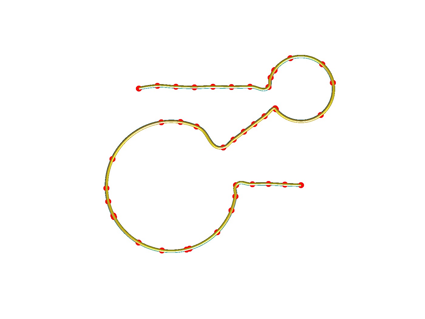
In Example 3.2 of Section 3.1, we already explained the local curve of the arc. One of the advantages of using arcs as local curves is that the curve is locally a circle if the dataset itself is intended to behave like a circle, see Figure 21.
In the case of three-dimensional space, one may need to adapt a curve on spherical data. Because we use the circular local function, we can always expect our local curves to be located on the sphere when the data cloud is on the sphere. When we glue the two local curves on a sphere, all we have to do is to use a special gluing function. For instance, when we glue two arcs on a sphere from to , see Figure 22. We can define , where and are two arcs pass and that we are going to glue. We can define as a series of arcs on the sphere pass and with uniform arc length so that and for all . For the direction, one can easily find that the center of these arcs will be located on a circle inside the sphere. Therefore, we can parametrize the direction by the center location of these arcs. More specifically, let be the center of the arc of and we choose to be a constant. In this way, we define the gluing function by , where is the blending function.
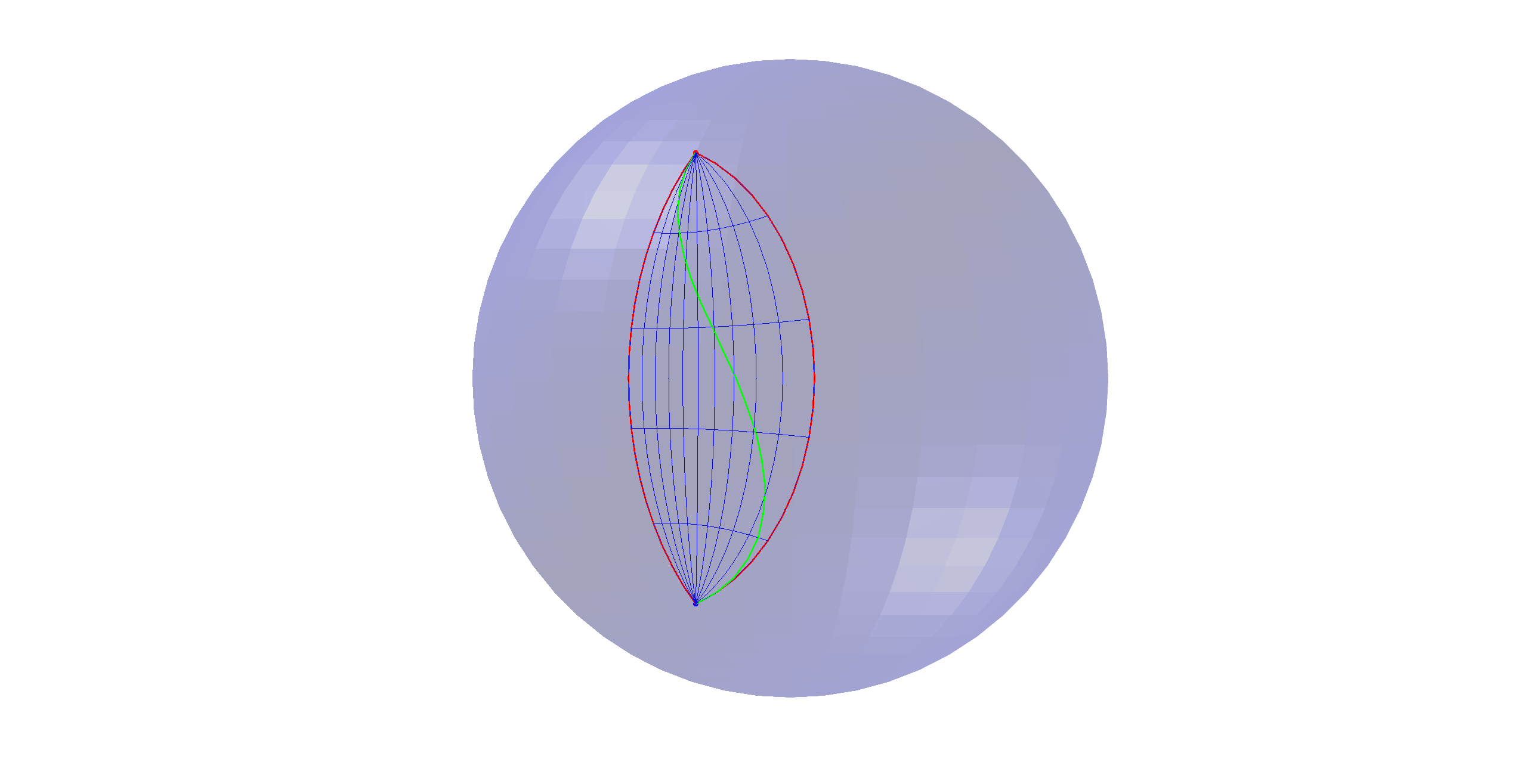
As shown in Figure 23, two curves are presented to demonstrate that our
interpolating curves will be on the corresponding spheres when the
given data points are on the spheres. We can see that the curve fits the sphere whenever the data points are on the sphere.
 |
 |
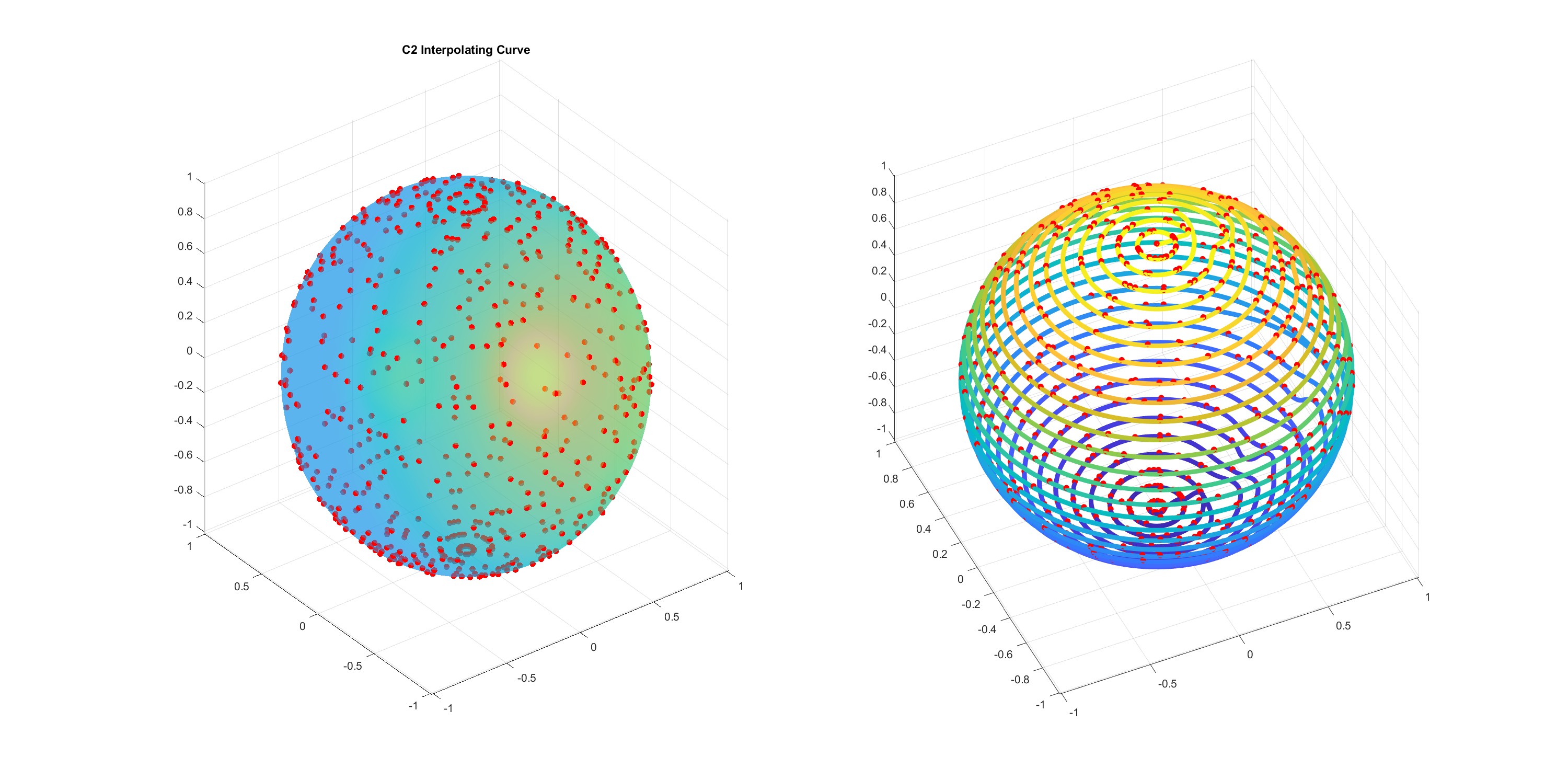
In the next example, we have a lot of points on the unit sphere. Our smooth interpolating curve is also on the same sphere as shown in Figure 24.
5 Conclusion and Future works
In this paper, we present an organized framework for constructing smoothly interpolating curves in with a high level of smoothness customization. While incorporating and refining existing approaches, our algorithm breaks down the smooth curve construction into four key components: the local function, blending function, distributing function, and gluing function.
The local function depends on the needs of shape design. One could use pure polynomials to simplify the calculation and save the storage, as shown in Example 4.1. In addition to the oriented points, some tangent vectors and normal vectors are
also given, we can modify our algorithm easily by
using local functions with derivative interpolation
properties.
Some useful local functions like circular functions in Example 3.2 and linear functions to preserve the convexity in Example 4.3 are also useful in various scenarios. Note that the local functions are not necessarily the same for all points. For instance, on the boundary, one may apply different boundary local functions to get the desired curve. In Example 4.2, we also show that by replacing the local function on the degenerated points, the curve can have the corner that we expected. In another example 4.3, we explained a convexity of the data points could be preserved if we use linear functions as local functions. The choice of local function is not limited to the example we have shown in this paper.
The Blending functions are used to determine the smoothness of the final curves. Applying -blending functions can give us a curve in most cases. We also saw that we can use the trigonometric function or other functions to replace the polynomial blending functions if they satisfy Definition 3.5.
The redistribution function maps the coordinate of the local function to a standard coordinate, which has one unit between each node. In this paper, we only use the piecewise linear map as our redistribution function. By Theorem 3.5, we may need our function after redistribution to be positive definite and regular. For the same local function, we could make the redistributed function positive definite by choosing a suitable redistribution function. The only non positive definite in this paper is the circular functions. However, Yuksel has proved that the curve is in his paper [7]. So, using the piecewise linear function in this case is fine.
When linear gluing may be a good choice, most of the time, we may need a different way to glue the two curves together. In Example 4.4, we demonstrate a special way to glue two curves together so that the final curve will locate on the same sphere as its original two curves. In the example, the gluing function does not affect the final smoothness because it is . If one uses other gluing functions, they may lose smoothness if the function is not smooth enough.
In this paper, we analyze previous works and decompose them into four parts of the function. Each part take there unique role in the construction of the final curve. We also indicated that the blending functions take an important role of smoothness. By providing -blending functions, we can now push the smoothness to any degree. We also give a necessary conditions that make the curve to be so when people use there preferred local function in our algorithm, they would expect a smooth curve as long as there formulate meets the condition.
Acknowledgments The authors are very grateful to the editor and referees for their helpful comments.
Declarations
-
•
Funding. The second author is supported by the Simons Foundation for collaboration grant #864439.
-
•
Competing interests. On behalf of all authors, the corresponding author states that there is no conflict of interest.
References
- \bibcommenthead
- DeRose [1985] DeRose, A.D.: Geometric continuity: A parametrization independent measure of continuity for computer aided geometric design. PhD thesis, EECS Department, University of California, Berkeley (Aug 1985). http://www2.eecs.berkeley.edu/Pubs/TechRpts/1985/6081.html
- Gregory [1989] Gregory, J.A.: Geometric Continuity. In: Lyche, T., Schumaker, L.L. (eds.) Mathematical Methods in Computer Aided Geometric Design, pp. 353–371. Academic Press, ??? (1989). https://doi.org/10.1016/B978-0-12-460515-2.50028-7 . https://www.sciencedirect.com/science/article/pii/B9780124605152500287 Accessed 2022-07-31
- Garrity and Warren [1991] Garrity, T., Warren, J.: Geometric continuity. Computer Aided Geometric Design 8(1), 51–65 (1991) https://doi.org/10.1016/0167-8396(91)90049-H . Accessed 2022-07-31
- Farin [1993] Farin, G.: Curves and Surfaces for Computer-Aided Geometric Design (Third Edition), Third edition edn., pp. 229–249. Academic Press, Boston (1993). https://doi.org/%****␣sn-article.bbl␣Line␣100␣****10.1016/B978-0-12-249052-1.50019-2 . https://www.sciencedirect.com/science/article/pii/B9780122490521500192
- Les Piegl [1995] Les Piegl, W.T.: The NURBS Book. Monographs in Visual Communication, vol. XIV, 646. Springer, Heidelberg (1995)
- Wenz [1996] Wenz, H.-J.: Interpolation of curve data by blended generalized circles. Computer Aided Geometric Design 13(8), 673–680 (1996) https://doi.org/10.1016/0167-8396(95)00054-2
- Yuksel [2020] Yuksel, C.: A class of c2 interpolating splines. ACM Transactions on Graphics 39(5), 160–116014 (2020) https://doi.org/10.1145/3400301
- Bertolazzi and Frego [2018] Bertolazzi, E., Frego, M.: On the g2 hermite interpolation problem with clothoids. Journal of Computational and Applied Mathematics 341, 99–116 (2018) https://doi.org/10.1016/j.cam.2018.03.029
- Knott [2000] Knott, G.D.: Function and Space Curve Interpolation, pp. 59–61. Birkhäuser Boston, Boston, MA (2000). https://doi.org/10.1007/978-1-4612-1320-8_4 . https://doi.org/10.1007/978-1-4612-1320-8_4
- Lee [1989] Lee, E.T.Y.: Choosing nodes in parametric curve interpolation. Computer-Aided Design 21(6), 363–370 (1989) https://doi.org/10.1016/0010-4485(89)90003-1
- Carmo [2016] Carmo, M.P.d.: Differential Geometry of Curves and Surfaces: Revised and Updated Second Edition. Courier Dover Publications, ??? (2016). Google-Books-ID: gg2xDQAAQBAJ
- Hu [2023] Hu, T.-W.: Computational methods for smooth mapping and interpolation using multivariate spline techniques. PhD thesis, University of Georgia (2023)