Limit theorems for Randić index for Erdős-Rényi graphs

Abstract

We prove that the generalized Randić index over graphs following the Erdős-Rényi model, for both the sparse and dense regimes, is concentrated around its mean when the number of vertices tends to infinity.

Keywords: Randić index, Erdős-Rényi graphs, topological indices, random graphs.

MSC classes: 05C50, 05C80

1 Introduction

A molecular graph, within the domain of chemistry, commonly represents the structure of a molecule graphically, with atoms as nodes and chemical bonds as edges connecting these nodes. Comprehending these structural representations is pivotal in pharmaceuticals for designing drugs, given that the arrangement of atoms and bonds significantly influences the molecule’s properties [31, 24]. In this sense, a numerical value, irrespective of the particular node and edge labeling, which encapsulates specific characteristics of the molecular graph, is termed a graph invariant or topological index. Hence, various topological indices and their mathematical properties have been explored [14, 15]. In particular, the Randić index emerges as the foremost extensively studied, commonly employed, and broadly acknowledged topological index [18, 20]; this is due to its close correlation with numerous chemical properties, including boiling points, surface area, solubility in water of alkanes [17, 28, 13]. It was initially termed as the “branching index” when introduced by chemist Milan Randić in 1975 [26] as

$$R(G)=\sum_{u\sim v}\frac{1}{\sqrt{d_{u}d_{v}}};$$

where the sum is over all the pairs of connected vertices $u\sim v$ of a graph $G$ and $d_{u},d_{v}$ stand for their respective degree (i.e. their number of connected neighbours in the graph). This index was later generalized by Bollobás and Erdős in 1998 [3], for $\alpha\in\mathbb{R}$,

$$R_{\alpha}(G)=\sum_{u\sim v}(d_{u}d_{v})^{\alpha}.$$ (1.1)

On the other hand, graph theory has shown to have applicability in representing and modeling various real-world systems as random graphs, as many of their crucial features are challenging to capture using deterministic models. In particular, a model of random graphs with a fixed number of vertices $n$ is a stochastic mechanism for determining which of the $n(n-1)/2$ potential edges actually arise. In 1959, the Erdős-Rényi (ER) random graph [11] was defined. In this graph, every pair of vertices is independently linked with probability $p$. When $p$ remains constant, it is termed as a dense ER graph. Conversely, if $p=O(1/n)$, it is referred to as a sparse ER graph. The properties of ER graphs have been thoroughly examined, including their largest independent sets, chromatic number, Hamiltonian paths, connected components, automorphisms, among others [16]. Additionally, in terms of applications, ER is essentially akin to an elementary model of an epidemic known as the Reed-Frost model, the findings regarding ER are beneficial for understanding evolutionarily stable strategies and, recently, some slight modifications of the original model serve as a significant foundation to model interactions within communities [25, 27]. In simpler terms, communities represent tightly-knit groups of nodes where interactions are frequent among members but less so with nodes outside the community. Hence, community analysis can reveal important patterns, decomposing large collections of interactions into more meaningful components. In general, although ER graphs are commonly recognized as suboptimal models for interaction networks, their simplicity, mathematical manageability, and relations with alternative models possessing real-world properties render them a valuable asset in network research and analysis.

Under the same line, several topological indices have been investigated within the ER model, employing computational or analytical approaches [19, 6, 23, 8]; since, for instance, comprehensive knowledge of various indices pertaining to the model could function as indicators of whether a network conforms to the Erdős-Rényi random graph model. Similarly, the generalized Randić index has been scrutinized across various random models [12, 34, 29, 30]. Moreover, as points of intersection, the generalized Randić index has been examined within the ER model [33, 22, 7]. Specifically, the generalized Randić index has been employed to estimate graph robustness and, at the same time, ER graphs have served as valuable benchmarks for evaluating graph robustness [7]. This measure, which indicates a graph’s capacity to sustain connectivity amidst node and edge loss, aids in examining the resilience of various systems. Inspired by the foregoing, the objective of this paper is to examine the asymptotic properties of the generalized Randić index in both dense and sparse scenarios through the application of the second moment method. Additionally, it aims to corroborate the empirical findings of previous studies and to show consistency with the theoretical results derived through different approaches.

2 Large number approximations

In this study, we exclusively focus on simple finite undirected graphs. A simple undirected graph is represented as $G=(V,E)$, where $E\subseteq V\times V$ is a set ensuring that $(v,v)\notin E$ for all $v\in V$, and if $(v,u)\in E$, then $(u,v)\in E$. Here, $V$ signifies the vertex set and $E$ represents the edge set. In a graph $G$, two vertices $u$ and $v$ are considered adjacent, or neighbors, if $(u,v)$ forms an edge in $G$, denoted as $u\sim v$. If all the vertices of $G$ are pairwise adjacent, then $G$ is complete. A complete graph on $n$ vertices is denotaded as $K_{n}$. The degree (or valency) $d_{v}$ of a vertex $v$ is the number of edges at $v$; this is equal to the number of neighbours of $v$. The number $\delta(G):=\min\{d_{v}\mid v\in V\}$ is the minimum degree of $G$, the number $\Delta(G):=\max\{d_{v}\mid v\in V\}$ its maximum degree.

We will work with the Erdős-Rényi random graph $G_{n,p}$ with parameters $n\in\mathbb{N}$ and $p\in(0,1)$. Vertices are labelled by $[n]=\{1,2,\ldots,n\}$. In this work we consider the generalized Randić index $R_{\alpha}(G_{n,p})$ with $\alpha\in\mathbb{R}$, as defined in (1.1). Recall that for the complete graph, $R_{\alpha}(K_{n})=\frac{n(n-1)^{1+2\alpha}}{2}$.

2.1 Sparse graphs

Let us first consider the case where $p=\lambda/n$ for $\lambda\in(0,\infty)$. Define, for a random variable $X=X_{\lambda}\stackrel{{\scriptstyle d}}{{=}}\mathrm{Poi}(\lambda)$ and $\alpha\in\mathbb{R}$,

$$c[\alpha,\lambda]=c_{\alpha,\lambda}={\mathbf{E}}\left[(1+X)^{\alpha}\right].$$

Theorem 2.1.

For $\lambda\in(0,\infty)$, the generalized Randić index of $G_{n,p}$ with parameter $\alpha\in\mathbb{R}$ is asymptotically concentrated around its mean. More precisely, as $n\to\infty$,

$$\frac{2R_{\alpha}(G_{n,p})}{n}=\frac{R_{\alpha}(G_{n,p})}{R_{-1/2}(K_{n})}\to\lambda c_{\alpha,\lambda}^{2},$$

in probability. Moreover, we observe that $\lambda c^{2}_{\alpha,\lambda}$ exhibits the same asymptotic behavior as $\lambda^{1+2\alpha}$ as $\lambda$ approaches infinity.

The proof of Theorem 2.1 is based on the second moment method and the following asymptotic expressions.

Lemma 2.2.

Let $\lambda\in(0,\infty)$, $\alpha\in\mathbb{R}$ and consider $G_{n,p}$ with $p=\lambda/n$. As $n\to\infty$,

$${\mathbf{E}}\left[(d_{1}d_{2})^{\alpha}|1\sim 2\right]\to c_{\alpha,\lambda}^{2}\qquad\text{and}\qquad{\mathbf{E}}\left[(d_{1}d_{2}d_{3}d_{4})^{\alpha}|1\sim 2,3\sim 4\right]\to c_{\alpha,\lambda}^{4}.$$

Proof.

Let $X^{(n)}_{i}$, $i=1,2$ be independent with $\mathrm{Bin}(n-2,\lambda/n)$ distribution. Conditional on $\{1\sim 2\}$, $d_{1}\stackrel{{\scriptstyle d}}{{=}}1+X^{(n)}_{1}$ and $d_{2}\stackrel{{\scriptstyle d}}{{=}}1+X^{(n)}_{2}$, thus we have

$${\mathbf{E}}\left[(d_{1}d_{2})^{\alpha}|1\sim 2\right]={\mathbf{E}}\left[\left(1+X^{(n)}_{1}\right)^{\alpha}\right]{\mathbf{E}}\left[\left(1+X^{(n)}_{2}\right)^{\alpha}\right]={\mathbf{E}}\left[\left(1+X^{(n)}_{1}\right)^{\alpha}\right]^{2}.$$

Since $X_{1}^{(n)}$ converges in distribution to $X$, a $\mathrm{Poi}(\lambda)$ r.v. and $f(x)=(1+x)^{\alpha}$ is continuous on $[0,\infty)$, then, $(1+X_{1}^{(n)})^{\alpha}$ converges in distribution to $(1+X)^{\alpha}$. At this point, let us check that $\{(1+X_{1}^{(n)})^{\alpha}\}_{n}$ is uniformly integrable. To see this, we have that

$${\mathbf{E}}\left[\left(1+X_{1}^{(n)}\right)^{\alpha}\right]=\displaystyle\sum_{k=0}^{n-2}(1+k)^{\alpha}\binom{n-2}{k}\left(\frac{\lambda}{n}\right)^{k}\left(1-\frac{\lambda}{n}\right)^{n-2-k}\leq\displaystyle\sum_{k=0}^{n-2}(1+k)^{\alpha}\frac{\lambda^{k}}{k!}.$$

Considering the convergence of the series in the r.h.s. by d’Alembert’s criterion, we deduce that

$$\sup_{n\in\mathbb{N}}{\mathbf{E}}\left[\left(1+X_{1}^{(n)}\right)^{\alpha}\right]<\infty.$$

This observation leads to the conclusion that $\{(1+X_{1}^{(n)})^{\alpha}\}_{n}$ is uniformly integrable, therefore, as $n\to\infty$

$${\mathbf{E}}\left[(d_{1}d_{2})^{\alpha}|1\sim 2\right]\to{\mathbf{E}}\left[(1+X)^{\alpha}\right]^{2}=c_{\alpha,\lambda}^{2}.$$ (2.1)

For the second statement, let $Y_{i}^{(n)}$, $1\leq i\leq 4$ be independent with $\mathrm{Bin}(n-4,\lambda/n)$ distribution. Similarly, conditional on $\{1\sim 2,3\sim 4\}$, $d_{i}\stackrel{{\scriptstyle d}}{{=}}1+\delta_{i}+Y_{i}^{(n)}$ where $\{\delta_{i}\}_{i\in[4]}$ are correlated random variables: $\delta_{i}={\mathbf{1}}_{[i\sim 3]}+{\mathbf{1}}_{[i\sim 4]}$ and $\delta_{i}={\mathbf{1}}_{[i\sim 1]}+{\mathbf{1}}_{[i\sim 2]}$, for $i=1,2$ and $i=3,4$, respectively. So, if let $A$ denote the event that there is at least one edge connecting the vertices in $\{1,2\}$ and $\{3,4\}$; since $A^{c}$ tells us that $\delta_{i}=0$ for all $1\leq i\leq 4$, it follows that

$${\mathbf{E}}\left[(d_{1}d_{2}d_{3}d_{4})^{\alpha}|1\sim 2,3\sim 4\right]$$

$$={\mathbf{E}}\left[(d_{1}d_{2}d_{3}d_{4})^{\alpha}|1\sim 2,3\sim 4,A^{c}\right]{\mathbf{P}}\left(A^{c}\right)+{\mathbf{E}}\left[(d_{1}d_{2}d_{3}d_{4})^{\alpha}|1\sim 2,3\sim 4,A\right]{\mathbf{P}}\left(A\right),$$

$$={\mathbf{E}}\left[\left(1+Y_{1}^{(n)}\right)^{\alpha}\right]^{4}(1-\frac{\lambda}{n})^{4}+{\mathbf{E}}\left[(d_{1}d_{2}d_{3}d_{4})^{\alpha}|1\sim 2,3\sim 4,A\right](1-(1-\frac{\lambda}{n})^{4}),$$

which completes the proof since the first summand converges using a similar argument as in (2.1), while the second summand goes to 0. ∎

Proof of Theorem 2.1.

In order to use the second moment method, it suffices to verify that, as $n\to\infty$,

$$\frac{2{\mathbf{E}}\left[R_{\alpha}(G_{n,p})\right]}{n\lambda c_{\alpha,\lambda}^{2}}\to 1\qquad\text{and}\qquad\frac{{\mathbf{E}}\left[R^{2}_{\alpha}(G_{n,p})\right]}{{\mathbf{E}}\left[R_{\alpha}(G_{n,p})\right]^{2}}\to 1.$$

The first limit follows from the exchangeability of the vertices in $G_{n,p}$ and Lemma 2.2, since

$${\mathbf{E}}\left[R_{\alpha}(G_{n,p})\right] =\binom{n}{2}{\mathbf{E}}\left[(d_{1}d_{2})^{\alpha}{\mathbf{1}}_{[1\sim 2]}\right]=\frac{\lambda(n-1)}{2}{\mathbf{E}}\left[(d_{1}d_{2})^{\alpha}|1\sim 2\right].$$

For the second limit, consider ${\mathbf{E}}\left[R^{2}_{\alpha}(G_{n,p})\right]$, which equals

$$6\binom{n}{4}{\mathbf{E}}\left[(d_{1}d_{2}d_{3}d_{4})^{\alpha}{\mathbf{1}}_{[1\sim 2]}{\mathbf{1}}_{[3\sim 4]}\right]+6\binom{n}{3}{\mathbf{E}}\left[(d_{1}^{2}d_{2}d_{3})^{\alpha}{\mathbf{1}}_{[1\sim 2]}{\mathbf{1}}_{[1\sim 3]}\right]+\binom{n}{2}{\mathbf{E}}\left[(d_{1}d_{2})^{2\alpha}{\mathbf{1}}_{[1\sim 2]}\right].$$

While

$$6\binom{n}{3}{\mathbf{E}}\left[(d_{1}^{2}d_{2}d_{3})^{\alpha}{\mathbf{1}}_{[1\sim 2]}{\mathbf{1}}_{[1\sim 3]}\right]+\binom{n}{2}{\mathbf{E}}\left[(d_{1}d_{2})^{2\alpha}{\mathbf{1}}_{[1\sim 2]}\right]=O(n),$$

the leading term, by Lemma 2.2, satisfies

$$6\binom{n}{4}n^{-2}{\mathbf{E}}\left[(d_{1}d_{2}d_{3}d_{4})^{\alpha}{\mathbf{1}}_{[1\sim 2]}{\mathbf{1}}_{[3\sim 4]}\right]=(1+O(n^{-1}))\frac{\lambda^{2}}{4}{\mathbf{E}}\left[(d_{1}d_{2}d_{3}d_{4})^{\alpha}|{\mathbf{1}}_{[1\sim 2]}{\mathbf{1}}_{[3\sim 4]}\right]\to\frac{\lambda^{2}c_{\alpha,\lambda}^{2}}{4};$$

which completes the proof of the second limit.

For completeness: Since $\frac{{\mathbf{E}}\left[R_{\alpha}(G_{n,p})\right]}{n}\to\frac{\lambda c_{\alpha,\lambda}^{2}}{2}$ as $n\to\infty$, it suffices to prove using Chebyshev’s inequality, that for $\varepsilon>0$,

$${\mathbf{P}}\left(|R_{\alpha}(G_{n,p})-{\mathbf{E}}\left[R_{\alpha}(G_{n,p})\right]|\geq\varepsilon{\mathbf{E}}\left[R_{\alpha}(G_{n,p})\right]\right)\leq\varepsilon^{-2}\frac{\mathrm{Var}(R_{\alpha}(G_{n,p}))}{{\mathbf{E}}\left[R_{\alpha}(G_{n,p})\right]^{2}}=\varepsilon^{-2}\left(\frac{{\mathbf{E}}\left[R^{2}_{\alpha}(G_{n,p})\right]}{{\mathbf{E}}\left[R_{\alpha}(G_{n,p})\right]^{2}}-1\right)\to 0;$$

as $n\to\infty$.

To confirm the last assertion for $\alpha\geq 0$, observe that $\lambda{\mathbf{E}}\left[(1+X)^{\alpha}\right]^{2}\geq\lambda$. For $\alpha<0$, coincidentally, using the same approach that will be detailed in Lemma 2.4, but employing the Chernoff Poisson bounds, we can verify that when $\lambda\to\infty$, $\lambda^{-\alpha}c_{\alpha,\lambda}\to 1$ (see, e.g., Section 2.2 in [4]). Consequently, the last statement is true. ∎

2.2 Dense graphs

The following analogous theorem holds for the case $p\in(0,1)$ fixed.

Theorem 2.3.

For $p\in(0,1)$, the generalized Randić index of $G_{n,p}$ with parameter $\alpha\in\mathbb{R}$ is asymptotically concentrated around its mean. More precisely, as $n\to\infty$,

$$\frac{2R_{\alpha}(G_{n,p})}{n^{2(1+\alpha)}}\sim\frac{R_{\alpha}(G_{n,p})}{R_{\alpha}(K_{n})}\to{p^{1+2\alpha}},$$

in probability.

The above theorem relies on the following lemma.

Lemma 2.4.

Let $\alpha\in\mathbb{R}$, $p\in(0,1)$ and consider $G_{n,p}$. As $n\to\infty$,

$$n^{-2\alpha}{\mathbf{E}}\left[(d_{1}d_{2})^{\alpha}|1\sim 2\right]\to p^{2\alpha}\qquad\text{and}\qquad n^{-4\alpha}{\mathbf{E}}\left[(d_{1}d_{2}d_{3}d_{4})^{\alpha}|1\sim 2,3\sim 4\right]\to p^{4\alpha}.$$

Proof.

Let $X^{(n)}\stackrel{{\scriptstyle d}}{{=}}\mathrm{Bin}(n-2,p)$ and $Y^{(n)}\stackrel{{\scriptstyle d}}{{=}}\mathrm{Bin}(n-4,p)$, it follows that

$${\mathbf{E}}\left[(d_{1}d_{2})^{\alpha}|1\sim 2\right]={\mathbf{E}}\left[\left(1+X^{(n)}\right)^{\alpha}\right]^{2},$$

and

$${\mathbf{E}}\left[\left(c_{1}+Y^{(n)}\right)^{\alpha}\right]^{4}\leq{\mathbf{E}}\left[(d_{1}d_{2}d_{3}d_{4})^{\alpha}|1\sim 2,3\sim 4\right]\leq{\mathbf{E}}\left[\left(c_{2}+Y^{(n)}\right)^{\alpha}\right]^{4},$$

where $c_{1}=1,3$ and $c_{2}=3,1$, for $\alpha\geq 0$ and $\alpha<0$, respectively. Thus, the proof boils down to establishing, for $X^{(n)}$ (and similarly, for $Y^{(n)}$) that

$$n^{-\alpha}{\mathbf{E}}\left[\left(1+X^{(n)}\right)^{\alpha}\right]\to p^{\alpha}.$$ (2.2)

According to the Weak Law of Large Numbers (WLLN), we have that $X^{(n)}/n$ converges to $p$ in probability. Hence, $(1+X^{(n)})/n$ converges to $p$ in probability and since $f(x)=x^{\alpha}$ is continuous on $(0,\infty)$, it is verified that $n^{-\alpha}(1+X^{(n)})^{\alpha}$ converges to $p^{\alpha}$ in probability. At this point, similarly, we are going to verify that $\{((1+X_{1}^{(n)})/n)^{\alpha}\}_{n}$ is uniformly integrable. It is worth noting that for $\alpha\geq 0$, verifying the statement is straightforward as $(1+X^{(n)})/n\leq 1$, for all $n$. Let’s check the case $\alpha<0$: To see this, let $\varepsilon\in(0,p)$ and define $A^{+}_{\varepsilon,n}=\{X^{(n)}\geq(p+\varepsilon)(n-2)\}$ and $A^{-}_{\varepsilon,n}=\{X^{(n)}\leq(p-\varepsilon)(n-2)\}$. Using Chernoff bounds (see, e.g. [16, Theorem 2.1] and [16, Corollary 2.2]) and that $\alpha<0$,

$$n^{-\alpha}{\mathbf{E}}\left[(1+X^{(n)})^{\alpha}{\mathbf{1}}_{[A^{+}_{\varepsilon,n}]}\right] \leq n^{-\alpha}{\mathbf{P}}\left(A^{+}_{\varepsilon,n}\right)\leq n^{-\alpha}e^{-\frac{\varepsilon^{2}(n-2)}{3p}},$$

$$n^{-\alpha}{\mathbf{E}}\left[(1+X^{(n)})^{\alpha}{\mathbf{1}}_{[A^{-}_{\varepsilon,n}]}\right] \leq n^{-\alpha}{\mathbf{P}}\left(A^{-}_{\varepsilon,n}\right)\leq n^{-\alpha}e^{-\frac{\varepsilon^{2}(n-2)}{2p}}.$$

Thus,

$$\lim_{n\to\infty}n^{-\alpha}{\mathbf{E}}\left[(1+X^{(n)})^{\alpha}{\mathbf{1}}_{[A^{+}_{\varepsilon,n}]}\right]=\displaystyle\lim_{n\to\infty}n^{-\alpha}{\mathbf{E}}\left[(1+X^{(n)})^{\alpha}{\mathbf{1}}_{[A^{-}_{\varepsilon,n}]}\right]=0.$$

On the other hand,

$$n^{-\alpha}{\mathbf{E}}\left[(1+X^{(n)})^{\alpha}{\mathbf{1}}_{[(A^{+}_{\varepsilon,n}\cup A^{-}_{\varepsilon,n})^{c}]}\right]\leq\left(\frac{1+(p-\varepsilon)(n-2)}{n}\right)^{\alpha}.$$

Therefore,

$$n^{-\alpha}{\mathbf{E}}\left[(1+X^{(n)})^{\alpha}\right]\leq(p-\epsilon)^{\alpha}+2\epsilon,$$

for $n\geq N_{\epsilon}$. This tells us that the desired sequence is uniformly integrable, since

$$\sup_{n\in\mathbb{N}}{\mathbf{E}}\left[\left(\frac{1+X^{(n)}}{n}\right)^{\alpha}\right]<\infty,$$

remember that $\varepsilon\in(0,p)$ is arbitrary. Therefore, the proof is completed. ∎

Proof of Theorem 2.3.

Analogously to the proof of Theorem 2.1, the exchangeability of the vertices in $G_{n,p}$ gives

$${\mathbf{E}}\left[R_{\alpha}(G_{n,p})\right] =\binom{n}{2}p{\mathbf{E}}\left[(d_{1}d_{2})^{\alpha}|1\sim 2\right],$$

and ${\mathbf{E}}\left[R^{2}_{\alpha}(G_{n,p})\right]$ equals to

$$6\binom{n}{4}p^{2}{\mathbf{E}}\left[(d_{1}d_{2}d_{3}d_{4})^{\alpha}|1\sim 2,3\sim 4\right]+6\binom{n}{3}p^{2}{\mathbf{E}}\left[(d_{1}^{2}d_{2}d_{3})^{\alpha}|1\sim 2,1\sim 3\right]+\binom{n}{2}p{\mathbf{E}}\left[(d_{1}d_{2})^{2\alpha}|1\sim 2\right].$$

So that by Lemma 2.4, as $n\to\infty$,

$$\frac{{\mathbf{E}}\left[R_{\alpha}(G_{n,p})\right]}{n^{2(1+\alpha)}}=(1+O(n^{-1}))\frac{pn^{-2\alpha}}{2}{\mathbf{E}}\left[(d_{1}d_{2})^{\alpha}|1\sim 2\right]\to\frac{p^{1+2\alpha}}{2},$$

and

$$\frac{{\mathbf{E}}\left[R^{2}_{\alpha}(G_{n,p})\right]}{n^{4(1+\alpha)}}=(1+O(n^{-1}))\frac{p^{2}n^{-4\alpha}}{4}{\mathbf{E}}\left[(d_{1}d_{2}d_{3}d_{4})^{\alpha}|1\sim 2,3\sim 4\right]+O(n^{-1})\to\frac{p^{2+4\alpha}}{4},$$

since, as in Lemma 2.4

$$n^{-4\alpha}{\mathbf{E}}\left[(d_{1}^{2}d_{2}d_{3})^{\alpha}|1\sim 2,1\sim 3\right]\to p^{4\alpha},$$

and

$$n^{-4\alpha}{\mathbf{E}}\left[(d_{1}d_{2})^{2\alpha}|1\sim 2\right]\to p^{4\alpha},$$

Therefore, the proof is established using the second moment method, as in the proof of Theorem 2.1. ∎

3 Discussion

Limit theorems for the classic Randić connectivity index can be derived from Theorems 2.1 and 2.3 by taking $\alpha=-1/2$. In the dense case, we observe that its asymptotic behavior is independent of the parameter $p$, i.e, its determination comes only from the structure; whereas the limits of its variations do fluctuate: as a function of $p$, the long-term behavior of the generalized Randić index is increasing for $-1/2<\alpha$ and decreasing for $\alpha<-1/2$. By the way, as a function of $\alpha$, the long-term behavior of the generalized Randić index is decreasing for $p\in(0,1)$. Throughout this section we define $L[\alpha,\lambda]=\lambda c^{2}_{\alpha,\lambda}.$

Corollary 3.1.

For both the dense and sparse case of ER graphs, the classic Randić index of $G_{n,p}$ is asymptotically concentrated around its mean. More precisely, as $n\to\infty$,

$$\frac{R_{-1/2}(G_{n,p})}{R_{-1/2}(K_{n})}\to L,$$

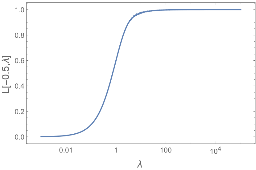
in probability, where $L=1$ for the dense case $(p\in(0,1))$ and $L=L[-1/2,\lambda]$ for sparse case $(p=\lambda/n,\lambda>0)$. Moreover, $L[-1/2,\lambda]$ converges to 1 as $\lambda\to\infty$.

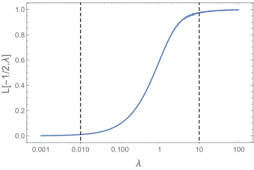
We can compare Corollary 3.1 with the results of [22], where the authors conducted a computational analysis of $R_{-1/2}(G)$ in the dense Erdős-Rényi model. Specifically, they plotted the average Randić index against the probability $p$ for various orders of $n$ and noted a transition from zero to $n/2$, with the rate of change increasing proportionally to $n$. This observation aligns well with the previous finding in the dense scenario. Additionally, when they re-plotted the curves as a function of $np$, they noticed that curves representing different graph sizes $n$ overlapped, forming a single universal curve. This observation, and even the asymptotic behaviour of the curve, can be further understood by considering our sparse results, which indicate that when the product $np=\lambda$ is constant, the classic Randić index over $n/2$ goes to a fixed value, and that it goes to 1 when $\lambda$ goes to infinity.

In fact, plotting $L[-1/2,\lambda]$ against $\lambda$ using a logarithmic scale (refer to Figure 3.1), we observe a curve consistent with the universal curve depicted in Figure 2(b) of [22]. This alignment enables the validation of the methodology proposed for predicting the classic Randić index’s value. Specifically, it delineates three distinct regimes: the predominantly isolated vertices regime ($\lambda<0.01$), the transitional regime ($0.01<\lambda<10$), and the regime characterized by nearly complete graphs ($\lambda>10$).

Figure 3.1: $L[-1/2,\lambda]$ as a function of $\lambda$, where the expectation was computed by averaging over 2000 random variables $Poi(\lambda)$.

When $\alpha=-1$, $R_{-1}$ is known as the second modified Zagreb index; which is related to the eigenvalues of the normalized Laplacian matrix of the graph [5]. Thus, limit theorems concerning the second modified Zagreb index can be obtained from Theorems 2.1 and 2.3 by setting $\alpha=-1$.

Corollary 3.2.

The modified second Zagreb index of $G_{n,p}$ is asymptotically concentrated around its mean. More precisely, as $n\to\infty$,

$$R_{-1}(G_{n,p})\to\frac{1}{2p},$$

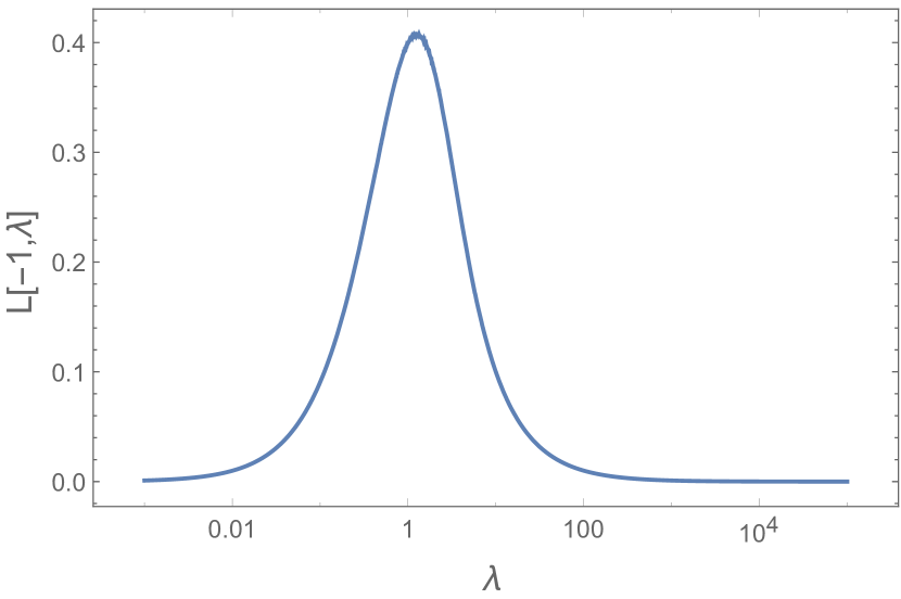
in probability, for the dense case. Moreover, $L[-1,\lambda]$ converges to 0 as $\lambda\to\infty$.

The following expression was derived in [7], for the expected value of $R_{-1}$ in the dense case,

$$\mathbb{E}[R_{-1}(G_{n,p})]=\frac{\left(1-(1-p)^{n+1}\right)^{2}}{2p}.$$

This result aligns with the previously mentioned observation that $R_{-1}$ asymptotically converges to its expectation.

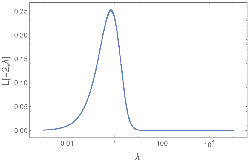
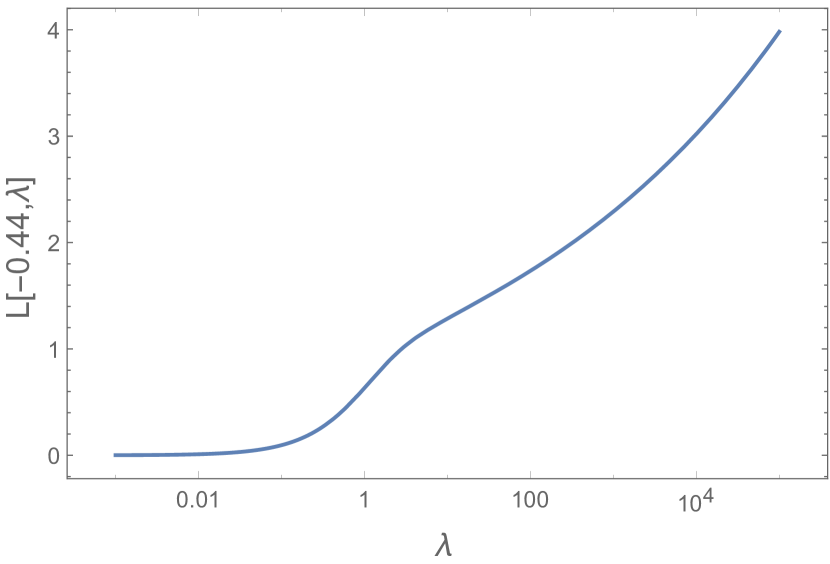
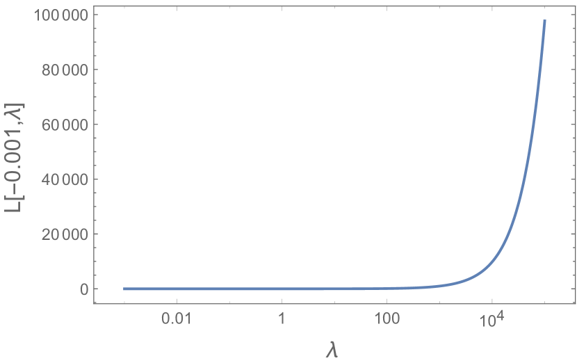
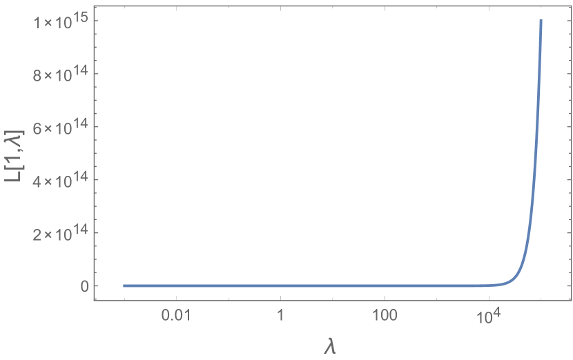
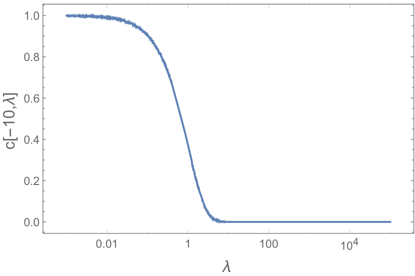
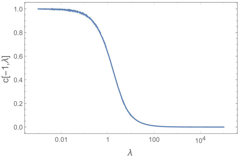
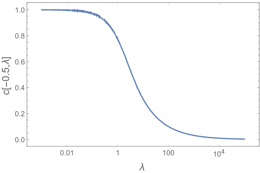
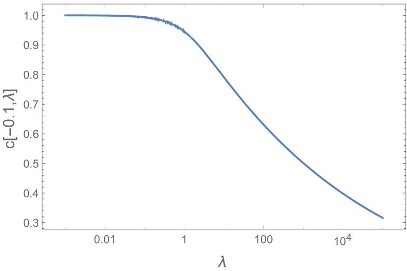
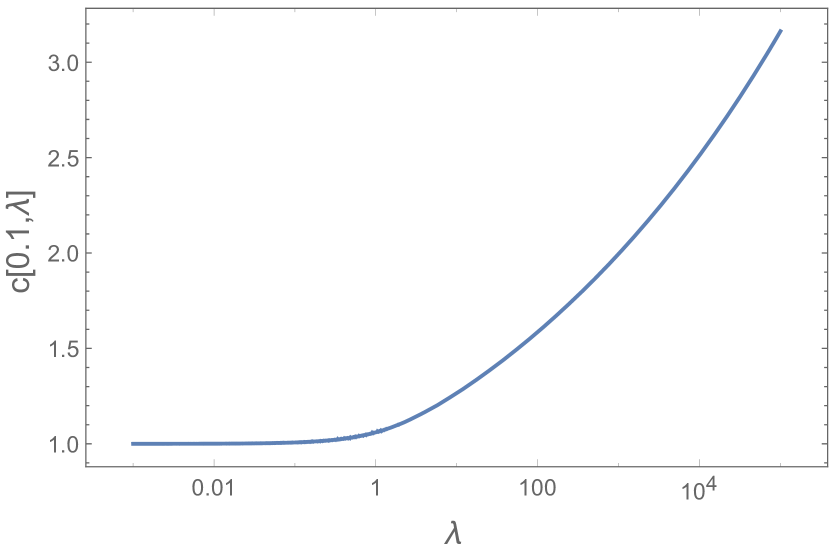
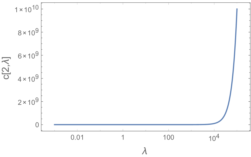
Inspired by the above analysis and in order to complement the main results, $L[\alpha,\lambda]$ and $c[\alpha,\lambda]$ are plotted as functions of $\lambda$ for some values of $\alpha$ in Figure 3.2 and Figure 3.3, respectively. Please note that the plot of $L[-1/2,\lambda]$ has already been depicted in Figure 3.1. Here, the average is computed over a sample of 2000 random variables $Poi(\lambda)$.

$\alpha=-2$

$\alpha=-1$

$\alpha=-0.5$

$\alpha=-0.44$

$\alpha=-0.001$

$\alpha=1$

Figure 3.2: $L[\alpha,\lambda]$ as a function of $\lambda$, where the average was calculated by averaging over 2000 random variables $Poi(\lambda)$.

$\alpha=-10$

$\alpha=-1$

$\alpha=-0.5$

$\alpha=-0.1$

$\alpha=0.1$

$\alpha=2$

Figure 3.3: $c[\alpha,\lambda]$ as a function of $\lambda$, where the expectation was computed by averaging over 2000 random variables $Poi(\lambda)$.

On the other hand, in a more recent work [33], the author employed primarily Taylor expansion and the Mean Value Theorem to study the generalized Randić index on an inhomogeneous Erdős–Rényi random graph (encompassing the classical Erdős–Rényi random graphs). Specifically, in Corollary 2.2, the author obtained that: with $np_{n}log(2)\geq log(n)$ (indicating an a.s connected graph), it follows that

$$R_{\alpha}(G_{n,p})=\frac{n^{2(1+\alpha)}p_{n}^{1+2\alpha}}{2}\left[1+O_{P}\left(\frac{\left(\log\left(np_{n}\right)\right)^{4(1-\alpha)_{+}}}{\sqrt{np_{n}}}\right)\right].$$

In the context provided, $X_{n}=O_{P}(a_{n})$ signifies that $X_{n}/a_{n}$ is bounded in probability. As expected, adopting an alternative and more reduced approach, we obtain more accurate results which are consistent with these findings.

Finally, at this point, it is important to emphasize that the identical process (or a slightly different tehcnik) can be utilized for analyze other topological indices derived from degree:

$$TI(G)=\displaystyle\sum_{v\sim u}F(d_{v},d_{u}),$$

such as:

• The atom - bond connectivity ($ABC$), where $F(x,y)=\sqrt{\frac{x+y-2}{xy}}.$

• The geometric - arithmetic index ($GA$), where $F(x,y)=\frac{2\sqrt{xy}}{x+y}.$

• The harmonic index ($H$), where $F(x,y)=\frac{2}{x+y}.$

• The sum - connectivity index ($\chi$), where $F(x,y)=\frac{1}{\sqrt{x+y}}.$

• The logarithm of first multiplicative Zagreb index, where $F(x,y)=2\left(\frac{\ln x}{x}+\frac{\ln y}{y}\right).$

As motivation, similarly, the aforementioned approach could offer us either theoretical support or a contrast for the findings obtained in [23, 7, 8, 21, 33]. Another noteworthy aspect is that the main findings may be beneficial to explore topological indices not conforming to the above form. Especially, the energy index of $G$, denoted as $\mathcal{E}(G)$ and defined by

$$\mathcal{E}(G)=Tr(|A(G)|),$$ (3.1)

can be examined. This is due to the results presented in [1] and [32], which establish that

$$2R_{-1/2}(G)\leq\mathcal{E}(G)\leq 2\sqrt{\Delta(G)}R_{-1/2}(G).$$

From that perspective, the implications of the observed long-run behavior of the classical Randić index of the Erdős-Rényi sparse random graph suggest the conjecture that $\mathcal{E}(G)/n\to g(\lambda)$ when $n\to\infty$. By the way, something similar was conjectured for the trees generated by the Barabasi-Albert model with parameter $\alpha$ in [2]; perhaps, the approach developed in this paper can be explored in the Barabasi-Albert model and coupled with equation (3.1) to say something about the asymptotic behavior of the energy. As an additional point, for the dense case, it is well known that almost all ER graphs over $n$ vertices have energy of order $n^{3/2}(\frac{8}{3\pi}\sqrt{p(1-p)}+o(1))$ [9]. Actually, since the adjacency matrix of a random graph is a random matrix, the proof relies on one of the most important achievements in this field which is Wigner’s semicircular law. In general, examining the classical Randić index of the Erdős-Rényi random graph can provide insight into the asymptotic trends of energy, such as hyperenergetic and hypoenergetic characteristics, and conversely [10].

Funding Information

Laura Eslava was supported by DGAPA-PAPIIT-UNAM grant IN-102822, Arno Siri-Jégousse was supported by DGAPA-PAPIIT-UNAM grant IN-102824 and Salyé Sigarreta was supported by CONAHCYT grant.

References

• [1] Arizmendi, G., and Arizmendi, O. (2021). Energy of a graph and Randić index. Linear Algebra and its Applications.
• [2] Arizmendi, O., and Dominguez, E. (2022). Barabasi–Albert trees are hypoenergetic. Boletín de la Sociedad Matemática Mexicana.
• [3] Bollobás, B. and Erdős, P. (1998). Graphs of extremal weights, Ars Combinatoria.
• [4] Boucheron, S., Lugosi, G., and Massart. P. (2013). Concentration inequalities. Oxford University Press, Oxford.
• [5] Cavers, M. S. (2010). The normalized Laplacian matrix and general Randić index of graphs. Faculty of Graduate Studies and Research, University of Regina.
• [6] Chen, R., Li, J., and He, W. (2022). Assessing Graph Robustness through Modified Zagreb Index. Axioms.
• [7] De Meo, P., Messina, F., Rosaci, D., Sarné, G. M., and Vasilakos, A. V. (2017). Estimating graph robustness through the Randić index. IEEE Transactions on Cybernetics.
• [8] Došlic, T., Hosseinzadeh, M. A., Hossein-Zadeh, S., Iranmanesh, A., and Rezakhanlou, F. (2020). On generalized Zagreb indices of random graphs. MATCH Communications in Mathematical and in Computer Chemistry.
• [9] Du, W., Li, X., and Li, Y. (2011). The energy of random graphs. Linear algebra and its applications.
• [10] Erdős, L., Knowles, A., Yau, H. T., and Yin, J. (2012). Spectral statistics of Erdős-Rényi graphs II: Eigenvalue spacing and the extreme eigenvalues. Communications in Mathematical Physics.
• [11] Erdős, P., and Rényi, A. (1959). On random graphs. I. Publicationes Mathematicae Debrecen.
• [12] Feng, Q., Mahmoud, H. M., and Panholzer, A. (2008). Limit laws for the Randić index of random binary tree models. Annals of the Institute of Statistical Mathematics.
• [13] Gnanaraj, L. R. M., Ganesan, D., and Siddiqui, M. K. (2023). Topological indices and QSPR analysis of NSAID drugs. Polycyclic Aromatic Compounds.
• [14] Gutman, I. (2013). Degree-based topological indices. Croatica Chemica Acta.
• [15] Gutman, I., and Furtula, B. (2017). Survey of graph energies. Mathematics Interdisciplinary Research.
• [16] Janson, S., Luczak, T., and Rucinski, A. (2011). Random graphs. John Wiley and Sons.
• [17] Kier, L. B., and Hall, L. H. (1986). Molecular connectivity in structure-activity analysis. Wiley, New York.
• [18] Li, X., Gutman, I., and Randić, M. (2006). Mathematical aspects of Randić-type molecular structure descriptors. University, Faculty of Science.
• [19] Li, X., Li, Y., and Song, J. (2020). The asymptotic value of graph energy for random graphs with degree-based weights. Discrete Applied Mathematics.
• [20] Li, X., and Shi, Y. (2008). A survey on the Randić index. MATCH Communications in Mathematical and in Computer Chemistry.
• [21] Li, S., Shi, L., and Gao, W. (2021). Two modified Zagreb indices for random structures. Main Group Metal Chemistry.
• [22] Martínez-Martínez, C. T., Mendez-Bermudez, J. A., Rodríguez, J. M., and Sigarreta, J. M. (2020). Computational and analytical studies of the Randić index in Erdös–Rényi models. Applied Mathematics and Computation.
• [23] Martinez-Martinez, C. T., Mendez-Bermudez, J. A., Rodriguez, J. M., and Sigarreta, J. M. (2021). Computational and Analytical Studies of the Harmonic Index on Erdős-Rényi Models. MATCH Communications in Mathematical and in Computer Chemistry.
• [24] Mukwembi, S., and Nyabadza, F. (2023). Predicting anti-cancer activity in flavonoids: a graph theoretic approach. Scientific Reports.
• [25] Penman, D. B., and Cannings, C. (2003). Models of random graphs and their applications. Handbook of Statistics.
• [26] Randić, M. (1975). On characterization of molecular branching. Journal of the American Chemical Society.
• [27] Seshadhri, C., Kolda, T. G., and Pinar, A. (2012). Community structure and scale-free collections of Erdős-Rényi graphs. Physical Review E.
• [28] Shigehalli, V. S., and Dsouza, A. M. (2022). Quantitative structure property relationship (qspr) analysis of general randić index. Journal of Algebraic Statistics.
• [29] Sigarreta, S., Sigarreta, S., and Cruz-Suárez, H. (2023). On Bond Incident Degree Indices of Random Spiro Chains. Polycyclic Aromatic Compounds.
• [30] Sigarreta, S. C., Sigarreta, S. M., and Cruz-Suárez, H. (2022). On degree–based topological indices of random polyomino chains. Mathematical Biosciences and Engineering.
• [31] Wei, J., Cancan, M., Rehman, A. U., Siddiqui, M. K., Nasir, M., Younas, M. T., and Hanif, M. F. (2022). On topological indices of remdesivir compound used in treatment of Corona virus (COVID 19). Polycyclic Aromatic Compounds.
• [32] Yan, Z., Liu, C., Pan, Y., and Li, J. (2021). Energy, Randić index and maximum degree of graphs. MATCH Communications in Mathematical and in Computer Chemistry.
• [33] Yuan, M. (2023). On the Randić index and its variants of network data. TEST.
• [34] Zhang, P., and Wang, X. (2022). Several topological indices of random caterpillars. Methodology and Computing in Applied Probability.