Boundary element methods for the magnetic field integral equation on polyhedra

Abstract

This paper provides a rigorous analysis on boundary element methods for the magnetic field integral equation on Lipschitz polyhedra. The magnetic field integral equation is widely used in practical applications to model electromagnetic scattering by a perfectly conducting body. The governing operator is shown to be coercive by means of the electric field integral operator with a purely imaginary wave number. Consequently, the continuous variational problem is uniquely solvable, given that the wave number does not belong to the spectrum of the interior Maxwell’s problem. A Galerkin discretization scheme is then introduced, employing Raviart-Thomas basis functions for the solution space and Buffa-Christiansen functions for the test space. A discrete inf-sup condition is proven, implying the unique solvability of the discrete variational problem. An asymptotically quasi-optimal error estimate for the numerical solutions is established, and the convergence rate of the numerical scheme is examined. In addition, the resulting matrix system is shown to be well-conditioned regardless of the mesh refinement. Some numerical results are presented to support the theoretical analysis.

31B10, 65N38

1 Introduction

The numerical computation of electromagnetic fields scattered by a perfectly conducting body $\Omega\subset\mathbb{R}^{3}$ usually leads to solving a Dirichlet boundary-value problem of the electric wave equation in the exterior unbounded domain $\Omega^{c}:=\mathbb{R}^{3}\setminus\overline{\Omega}$, supplemented with the Silver-Müller radiation condition at infinity. Based on the Stratton-Chu representation formula, it boils down to solving one of two standard boundary integral equations, namely the electric field integral equation (EFIE) and the magnetic field integral equation (MFIE).

With boundary element methods (BEMs) in mind, we assume that the domain $\Omega$ is a polyhedron with Lipschitz continuous boundary $\Gamma:=\partial\Omega$ that only consists of plane faces $\Gamma_{j}$, $j=1,2,\ldots,N_{F}$. The extension of the results to Lipschitz curvilinear polyhedra is straightforward. On polyhedral boundary $\Gamma$, the definition of Sobolev spaces $\operatorname{H}^{s}(\Gamma)$, in particular with $\left|{s}\right|\geq 1$, and differential operators are not obvious as those on smooth surfaces. By localization to each face $\Gamma_{j}$, Buffa and Ciarlet successfully developed functional setting for Maxwell’s equations on Lipschitz polyhedra, where tangential traces of vector fields in $\operatorname{\mathbf{H}}(\textbf{{curl}},\Omega)$, their trace spaces and relevant surface differential operators were properly characterized [1, 3, 4]. All ingredients necessary to develop a standard functional theory, including integration by parts formulas and Hodge decompositions, were also provided. A generalization for general Lipschitz domains was then presented in [6].

Based on the developed functional theory for Maxwell’s equations on Lipschitz domains, a natural BEM for the EFIE on polyhedra was studied in [22]. The continuous and discrete variational problems are coercive with respect to continuous and semidiscrete Hodge decompositions, respectively. The Galerkin discretization of the EFIE employing Raviart-Thomas boundary elements was analyzed, exhibiting the quasi-optimal convergence of numerical solutions. Another discretization scheme for the EFIE on non-smooth Lipschitz domains was proposed in [5], which is based on standard boundary elements rather than Raviart-Thomas elements. On polyhedral surfaces, an asymptotically quasi-optimal convergence behaviour was also achieved. BEMs for Maxwell transmission problems on Lipschitz domains were investigated in [9]. The Galerkin discretization with Raviart-Thomas spaces was considered, and the results were applied to electromagnetic scattering by perfect electric conductors and by dielectric bodies. In the case of the perfect conductor scattering, only the EFIE was examined, also yielding quasi-optimal numerical solutions. To determine the actual rate of convergence on polyhedral domains, the singularities of solution to Maxwell’s equations must also be taken into account [17]. More specifically, the convergence rate of BEMs for the EFIE is limited by the regularity parameter $s^{\ast}$ of the Laplace-Beltrami operator on $\Gamma$, which depends on the geometry of $\Gamma$ in neighborhoods of vertices only, see, e.g., [22, 5].

In addition to the EFIE, BEMs for combined field integral equations (CFIEs) on Lipschitz domains were investigated in [8, 25]. When the wave number belongs to the spectrum of the interior Maxwell’s problem, the EFIE and MFIE are not uniquely solvable, resulting in resonant instabilities of Galerkin discretization systems. CFIEs owe their name to an appropriate combination of the Maxwell single and double layer potentials, thereby getting rid of the spurious resonances. In [8], the authors exploited the coercivity of the EFIE operator by applying a compact regularization to the double layer part. The continuous and discrete variational problems were proven to be uniquely solvable at all wave numbers. A Galerkin boundary element discretization was proposed, whose numerical solutions satisfy an asymptotically quasi-optimal error estimate. The paper [25] introduced a preconditioned CFIE on which the EFIE and MFIE operators are preconditioned by their counterparts of a purely imaginary wave number. By means of a Calderón projection formula, the governing CFIE operator was cast into an equivalent formulation that, up to a compact perturbation, is $S_{i\kappa}$-coercive, with $S_{i\kappa}$ the EFIE operator of purely imaginary wave number $i\kappa$. A Galerkin discretization of the mixed variational problem using the lowest-order Raviart-Thomas space and its dual Buffa-Christiansen space was analyzed, producing quasi-optimal numerical solutions. Moreover, the resulting matrix systems were shown to be well-conditioned on fine meshes and stable at resonant frequencies. Nonetheless, the proposed discretization scheme in [25] is not the one typically used by practitioners. In practice, the MFIE part of the CFIE is commonly discretized using Raviart-Thomas basis functions for the solution space and Buffa-Christiansen functions for the test space [28, 27, 26].

This paper aims to provide a rigorous analysis on BEMs for the MFIE on Lipschitz polyhedra. Like the EFIE and CFIEs, the MFIE is widely used in practical applications to model the electromagnetic scattering by perfect electric conductors. Despite its utility, however, attention paid to the MFIE is not at the same level with those for the EFIE and CFIEs. This is evident in the relatively limited number of papers devoting to BEMs for the MFIE, with most of them contributed by practitioners, see, e.g., [32, 18, 19, 15, 23, 24]. On smooth surfaces, the MFIE operator is well-known to be a Fredholm operator of second kind [7]. The existence and uniqueness of a solution to the continuous variational problem of the MFIE has been shown for smooth domains, provided that the wave number is not an eigenvalue of the interior Maxwell’s problem, see, e.g., [7]. In the discrete setting, this is not even necessarily true, since the boundary element subspace may not be dual to itself. More precisely, the Galerkin discretization of the identity operator (the principal part) occurring in the MFIE using lowest-order Raviart-Thomas elements has been proven to not satisfy the discrete inf-sup condition, see [11, Section 3.1]. As a result, the coercivity of the corresponding Galerkin discretization of the MFIE does not hold true.

The contribution of this paper is twofold. Firstly, we prove that the continuous variational problem of the MFIE is also uniquely solvable on Lipschitz domains, of course provided that the wave number does not belong to the spectrum of the interior Maxwell’s problem. This is done by means of the elliptic operator $S_{i\kappa}$. More particularly, we show that the MFIE operator is $S_{i\kappa}$-coercive up to a compact perturbation. It is noteworthy that on non-smooth Lipschitz surfaces, the average of exterior and interior double layer boundary integral operators is not necessarily compact. Secondly, we analyze the mixed discretization scheme for the MFIE introduced in [15], when the boundary $\Gamma$ is Lipschitz continuous. The authors of [15] proposed a Galerkin discretization of the MFIE employing Raviart-Thomas basis functions for the solution space and Buffa-Christiansen functions for the test space, on which they exploited the duality between the Buffa-Christiansen space and the Raviart-Thomas space [2]. Given that the average double layer boundary integral operator is compact on smooth surfaces, this duality supplies the coercivity. Fortunately, the coercivity of the mixed discretization of the MFIE remains valid when the surface is solely Lipschitz continuous, thanks to the $S_{i\kappa}$-coercivity of the MFIE operator. As a consequence, the asymptotic quasi-optimality of numerical solutions is obtained. In addition, we show that the resulting matrix system is well-conditioned regardless of the boundary mesh refinement. To end this paragraph, we state here the following essential assumption and stop repeating it in the remainder of the paper. The wave number is bounded away from the spectrum of the interior Maxwell’s problem.

This paper is organized as follows. The next section recalls the standard functional setting for Maxwell’s equations on Lipschitz polyhedra, including the tangential trace operators, trace spaces, relevant tangential differential operators and an integration by parts formula. Section 3 gives the definition and properties of Maxwell potentials and boundary integral operators. The MFIE and its variational formulation are derived in Section 4. The $S_{i\kappa}$-coercivity of the MFIE operator is proven for Lipschitz domains, implying the unique solvability of the continuous variational problem. In Section 5, we analyze a Galerkin boundary element discretization of the MFIE. Its solvability, an asymptotically quasi-optimal error estimate for discrete solutions and the bounded condition number of the matrix system are established in this section. Some numerical results are presented in Section 6, aiming to verify the numerical analysis. Finally, we provide some conclusion remarks and discuss some possibilities for future works in Section 7.

2 Function spaces

In this section, we briefly recall the functional setting for Maxwell’s equations on Lipschitz polyhedra. For more details and proofs, we refer the reader to the articles [1, 3, 4, 6]. Throughout the paper, regular symbols are used for scalar functions and their spaces, while bold symbols are used for vector fields and vector spaces.

Let $\Omega\subset\mathbb{R}^{3}$ be a bounded polyhedron with Lipschitz continuous boundary $\Gamma$, which only consists of flat faces $\Gamma_{j}$, $j=1,2,\ldots,N_{F}$, i.e., $\overline{\Gamma}=\bigcup_{j}\overline{\Gamma_{j}}$. The unbounded complement $\Omega^{c}:=\mathbb{R}^{3}\setminus\overline{\Omega}$ and the unit normal vector $\textbf{n}\in\operatorname{\mathbf{L}}^{\infty}(\Gamma)$ pointing from $\Omega$ to $\Omega^{c}$. On the polyhedral boundary $\Gamma$, the usual Sobolev spaces $\operatorname{H}^{s}(\Gamma)$ are defined invariantly for $s\in[0,1]$, with convention $\operatorname{H}^{0}(\Gamma)\equiv\operatorname{L}^{2}(\Gamma)$ [20, Section 1.3.3]. For $s>1$, the spaces $\operatorname{H}^{s}(\Gamma)$ can be characterized face by face, with a careful treatment at their common edges, see [3, 4]. We denote by $\operatorname{H}^{-s}(\Gamma)$ the dual space of $\operatorname{H}^{s}(\Gamma)$, and $\left\langle{\cdot,\cdot}\right\rangle_{s,\Gamma}$ their duality pairing. In addition, we introduce the space $\operatorname{H}^{3/2}_{\sim}(\Gamma):=\gamma(\operatorname{H}^{2}(\Omega))$ and its dual $\operatorname{H}^{-3/2}_{\sim}(\Gamma)$, with $\gamma$ the standard trace operator. The duality pairing between $\operatorname{H}_{\sim}^{-3/2}(\Gamma)$ and $\operatorname{H}_{\sim}^{3/2}(\Gamma)$ is denoted by $\left\langle{\cdot,\cdot}\right\rangle_{\sim,3/2,\Gamma}$. Here, we make the usual identification $\operatorname{L}^{2}(\Gamma)\subset\operatorname{H}^{-s}(\Gamma)$ and $\operatorname{L}^{2}(\Gamma)\subset\operatorname{H}^{-3/2}_{\sim}(\Gamma)$ via the $\operatorname{L}^{2}(\Gamma)$-pairing.

Next, we introduce the tangential trace operator $\gamma_{D}$, which is defined for smooth vector fields $\boldsymbol{u}\in\operatorname{\mathbf{C}}^{\infty}(\overline{\Omega})$ by

$$(\gamma_{D}\boldsymbol{u})(\boldsymbol{x})=\boldsymbol{u}(\boldsymbol{x})\times\textbf{n}(\boldsymbol{x}),$$

for almost all $\boldsymbol{x}\in\Gamma$. This operator can be extended to a continuous mapping from $\operatorname{\mathbf{H}}(\textbf{{curl}},\Omega)$ to $\operatorname{\mathbf{H}}^{-1/2}(\Gamma)$, see [20, Theorem 1.5.1.1]. In order to determine the actual range of $\gamma_{D}$, we adopt the definition $\operatorname{\mathbf{H}}^{s}_{\times}(\Gamma):=\gamma_{D}(\operatorname{\mathbf{H}}^{s+1/2}(\Omega))$, with $s\in(0,1)$, from [8, Definition 2.1]. For $s=0$, we set the space $\operatorname{\mathbf{H}}^{0}_{\times}(\Gamma)$ identical with

$$\operatorname{\mathbf{L}}^{2}_{\textbf{t}}(\Gamma):=\left\{{\boldsymbol{u}\in\operatorname{\mathbf{L}}^{2}(\Gamma):\boldsymbol{u}\cdot\textbf{n}=0}\right\},$$

which is endowed with the anti-symmetric pairing

$$\left\langle{\boldsymbol{u},\boldsymbol{v}}\right\rangle_{\times,\Gamma}:=\int_{\Gamma}(\boldsymbol{u}\times\textbf{n})\cdot\boldsymbol{v}\,\mathrm{d}s,$$

for all $\boldsymbol{u},\boldsymbol{v}\in\operatorname{\mathbf{L}}^{2}_{\textbf{t}}(\Gamma)$. The dual space of $\operatorname{\mathbf{H}}^{s}_{\times}(\Gamma)$ is denoted by $\operatorname{\mathbf{H}}^{-s}_{\times}(\Gamma)$, whose elements are identified via the $\operatorname{\mathbf{L}}^{2}_{\textbf{t}}(\Gamma)$-pairing $\left\langle{\cdot,\cdot}\right\rangle_{\times,\Gamma}$.

Let us introduce relevant surface differential operators. The surface operator $\textbf{{curl}}_{\Gamma}:\widetilde{\operatorname{H}}^{3/2}(\Gamma)\to\operatorname{\mathbf{H}}^{1/2}_{\times}(\Gamma)$ can be defined by

$$\textbf{{curl}}_{\Gamma}\gamma(\varphi)=\gamma_{D}(\textbf{grad}\varphi),$$

for all $\varphi\in\operatorname{H}^{2}(\Omega)$, see [6, Proposition 3.4]. Then, the surface divergence operator $\textup{div}_{\Gamma}:\operatorname{\mathbf{H}}^{-1/2}_{\times}(\Gamma)\to\operatorname{H}^{3/2}_{\sim}(\Gamma)$ is defined as dual to $\textbf{{curl}}_{\Gamma}$ in the sense

$$\left\langle{\textup{div}_{\Gamma}\boldsymbol{u},\varphi}\right\rangle_{\sim,3/2,\Gamma}=-\left\langle{\boldsymbol{u},\textbf{{curl}}_{\Gamma}\varphi}\right\rangle_{1/2,\Gamma},$$

for all $\boldsymbol{u}\in\operatorname{\mathbf{H}}^{-1/2}_{\times}(\Gamma)$ and $\varphi\in\widetilde{\operatorname{H}}^{3/2}(\Gamma)$. Now, we are able to introduce the space

$$\operatorname{\mathbf{H}}^{-1/2}_{\times}(\textup{div}_{\Gamma},\Gamma):=\left\{{\boldsymbol{u}\in\operatorname{\mathbf{H}}^{-1/2}_{\times}(\Gamma):\textup{div}_{\Gamma}\boldsymbol{u}\in\operatorname{H}^{-1/2}(\Gamma)}\right\},$$

equipped with the graph norm

$$\left\lVert{\boldsymbol{u}}\right\rVert^{2}_{\operatorname{\mathbf{H}}^{-1/2}_{\times}(\textup{div}_{\Gamma},\Gamma)}:=\left\lVert{\boldsymbol{u}}\right\rVert^{2}_{\operatorname{\mathbf{H}}^{-1/2}_{\times}(\Gamma)}+\left\lVert{\textup{div}_{\Gamma}\boldsymbol{u}}\right\rVert^{2}_{\operatorname{H}^{-1/2}(\Gamma)}.$$

The next theorem presents the extension of the $\operatorname{\mathbf{L}}^{2}_{\textbf{t}}(\Gamma)$-pairing $\langle{\cdot,\cdot}\rangle_{\times,\Gamma}$ to the space $\operatorname{\mathbf{H}}^{-1/2}_{\times}(\textup{div}_{\Gamma},\Gamma)$ and its self-duality with respect to this pairing, see, e.g., [4] and [6, Lemma 5.6].

Theorem 2.1 (self-duality of the space $\operatorname{\mathbf{H}}^{-1/2}_{\times}(\textup{div}_{\Gamma},\Gamma)$).

The pairing $\langle{\cdot,\cdot}\rangle_{\times,\Gamma}$ can be extended to a continuous bilinear form on the space $\operatorname{\mathbf{H}}^{-1/2}_{\times}(\textup{div}_{\Gamma},\Gamma)$. Moreover, $\operatorname{\mathbf{H}}^{-1/2}_{\times}(\textup{div}_{\Gamma},\Gamma)$ becomes its own dual with respect to $\langle{\cdot,\cdot}\rangle_{\times,\Gamma}$.

The tangential trace operator $\gamma_{D}$ maps from $\operatorname{\mathbf{H}}(\textbf{{curl}},\Omega)$ onto $\operatorname{\mathbf{H}}^{-1/2}_{\times}(\textup{div}_{\Gamma},\Gamma)$, making it the natural trace space for electromagnetic fields. The following theorem provides an integration by parts formula, which is essential for further analysis in this paper, see [6, Theorem 4.1] or [13, Theorem 2.3].

Theorem 2.2 (integration by parts formula).

The tangential trace operator $\gamma_{D}$ continuously maps from $\operatorname{\mathbf{H}}(\textbf{{curl}},\Omega)$ onto $\operatorname{\mathbf{H}}^{-1/2}_{\times}(\textup{div}_{\Gamma},\Gamma)$, which possesses a continuous right inverse. In addition, the following integration by parts formula holds for all $\boldsymbol{u},\boldsymbol{v}\in\operatorname{\mathbf{H}}(\textbf{{curl}},\Omega)$

(1) $$\int_{\Omega}(\textbf{{curl}}\,\boldsymbol{u}\cdot\boldsymbol{v}-\boldsymbol{u}\cdot\textbf{{curl}}\,\boldsymbol{v})\,\mathrm{d}\boldsymbol{x}=-\left\langle{\gamma_{D}\boldsymbol{u},\gamma_{D}\boldsymbol{v}}\right\rangle_{\times,\Gamma}.$$

When investigating the convergence rate of BEMs, higher regularities of the solution are required. The definition of the spaces $\operatorname{\mathbf{H}}^{s}_{\times}(\textup{div}_{\Gamma},\Gamma)$, with $s>-\tfrac{1}{2}$, can be found in [22, 8]. We omit those definitions for the sake of conciseness. Finally, we introduce the Neumann trace operator $\gamma_{N}:=\gamma_{D}\circ\textbf{{curl}}$, which continuously maps from $\operatorname{\mathbf{H}}(\textbf{{curl}}^{2},\Omega)$ onto $\operatorname{\mathbf{H}}^{-1/2}_{\times}(\textup{div}_{\Gamma},\Gamma)$, see [8].

3 Boundary integral operators

In this paper, we consider the scattering of time-harmonic electromagnetic fields with angular frequency $\omega>0$. The exterior region $\Omega^{c}$ is assumed to be filled by a homogeneous, isotropic and linear material with constant permittivity $\epsilon>0$ and permeability $\mu>0$. The wave number is defined by $\kappa:=\omega\sqrt{\epsilon\mu}>0$. In aid of further analysis with integral operators of a purely imaginary wave number, we state “the electric wave equation” and the Silver-Müller radiation condition with wave number $\sigma$, which can be either $\kappa$ or $i\kappa$,

(2) $$\,\,\textbf{{curl}}\,\textbf{{curl}}\,\boldsymbol{e}-\sigma^{2}\boldsymbol{e}=\boldsymbol{0}\qquad\qquad\qquad\text{in}\quad\Omega\cup\Omega^{c},$$

(3) $$\lim_{r\to\infty}\int_{\partial B_{r}}\left|{\textbf{{curl}}\,\boldsymbol{e}\times\textbf{n}+i\sigma(\textbf{n}\times\boldsymbol{e})\times\textbf{n}}\right|^{2}\,\mathrm{d}s=0.$$

Here, $\boldsymbol{e}$ is the unknown complex-valued vector field, $i$ stands for the imaginary unit, and $B_{r}$ denotes the ball of radius $r>0$ centered at $\boldsymbol{0}$.

When $\sigma=\kappa$, the problem (2)-(3), in conjunction with the Dirichlet boundary condition

(4) $$\boldsymbol{e}\times\textbf{n}=-\boldsymbol{e}^{in}\times\textbf{n}\qquad\qquad\text{on}\quad\Gamma,$$

describes the perfect conductor scattering at the boundary $\Gamma$ [14, Section 6.4]. In this case, the unknown $\boldsymbol{e}$ represents the scattered electric field, and the incident electric field $\boldsymbol{e}^{in}$ plays the role of excitation. The exterior problem has a unique solution $\boldsymbol{e}$ for all wave number $\kappa$ according to Rellich’s lemma [10, 29], whereas the interior problem is only uniquely solvable if $\kappa^{2}$ does not coincide with one of the Dirichlet or Neumann eigenvalues of the curl curl-operator inside $\Omega$.

When $\sigma=i\kappa$, the equation (2) is called the Yukawa-type equation. More details on the properties of integral operators associated with this equation can be found in [29, Section 5.6.4], [21, Section 5.1] and [34].

We denote by $G_{\sigma}(\boldsymbol{x},\boldsymbol{y})$ the fundamental solution associated with $\Delta+\sigma^{2}$, i.e.,

$$G_{\sigma}(\boldsymbol{x},\boldsymbol{y}):=\dfrac{\exp(i\sigma\left|{\boldsymbol{x}-\boldsymbol{y}}\right|)}{4\pi\left|{\boldsymbol{x}-\boldsymbol{y}}\right|},$$

for $\boldsymbol{x}\neq\boldsymbol{y}$. Then, the scalar and vectorial single layer potentials are respectively defined by

$$\Psi^{\sigma}_{V}(\varphi)(\boldsymbol{x}):=\int_{\Gamma}\varphi(\boldsymbol{y})G_{\sigma}(\boldsymbol{x},\boldsymbol{y})\,\mathrm{d}s(\boldsymbol{y}),\qquad\boldsymbol{\Psi}^{\sigma}_{\boldsymbol{A}}(\boldsymbol{u})(\boldsymbol{x}):=\int_{\Gamma}\boldsymbol{u}(\boldsymbol{y})G_{\sigma}(\boldsymbol{x},\boldsymbol{y})\,\mathrm{d}s(\boldsymbol{y}),$$

with $\boldsymbol{x}\notin\Gamma$. In the electromagnetic scattering problem, we are more interested in the Maxwell single and double layer potentials

$$\boldsymbol{\Psi}^{\sigma}_{SL}(\boldsymbol{u}):=\boldsymbol{\Psi}^{\sigma}_{\boldsymbol{A}}(\boldsymbol{u})+\dfrac{1}{\sigma^{2}}\textbf{grad}\,\Psi^{\sigma}_{V}(\textup{div}_{\Gamma}\boldsymbol{u}),\qquad\quad\boldsymbol{\Psi}^{\sigma}_{DL}(\boldsymbol{u}):=\textbf{{curl}}\,\boldsymbol{\Psi}^{\sigma}_{\boldsymbol{A}}(\boldsymbol{u}),$$

which continuously map $\operatorname{\mathbf{H}}^{-1/2}_{\times}(\textup{div}_{\Gamma},\Gamma)$ into $\operatorname{\mathbf{H}}_{\textup{loc}}(\textbf{{curl}}^{2},\Omega\cup\Omega^{c})$, see [21, Theorem 17]. For any $\boldsymbol{u}\in\operatorname{\mathbf{H}}^{-1/2}_{\times}(\textup{div}_{\Gamma},\Gamma)$, $\boldsymbol{\Psi}^{\sigma}_{SL}(\boldsymbol{u})$ and $\boldsymbol{\Psi}^{\sigma}_{DL}(\boldsymbol{u})$ are solutions to the problem (2)-(3). Therefore, it immediately holds that

(5) $$\textbf{{curl}}\circ\boldsymbol{\Psi}^{\sigma}_{SL}=\boldsymbol{\Psi}^{\sigma}_{DL},\qquad\qquad\quad\textbf{{curl}}\circ\boldsymbol{\Psi}^{\sigma}_{DL}=\sigma^{2}\boldsymbol{\Psi}^{\sigma}_{SL}.$$

On the other hand, any solution $\boldsymbol{u}\in\operatorname{\mathbf{H}}_{\textup{loc}}(\textbf{{curl}}^{2},\Omega\cup\Omega^{c})$ to the problem (2)-(3) satisfies the Stratton-Chu representation formula (see, e.g., [14, Theorem 6.2], [29, Theorem 5.5.1] and [21, Theorem 22])

(6) $$\boldsymbol{u}(\boldsymbol{x})=-\boldsymbol{\Psi}^{\sigma}_{DL}(\left[\gamma_{D}\right]_{\Gamma}\boldsymbol{u})(\boldsymbol{x})-\boldsymbol{\Psi}^{\sigma}_{SL}(\left[\gamma_{N}\right]_{\Gamma}\boldsymbol{u})(\boldsymbol{x}),$$

for $\boldsymbol{x}\in\Omega\cup\Omega^{c}$, where $\left[\gamma\right]_{\Gamma}:=\gamma^{+}-\gamma^{-}$ is the jump of some trace $\gamma$ across the boundary $\Gamma$, and the superscripts $-$ and $+$ designate traces onto $\Gamma$ from $\Omega$ and $\Omega^{c}$, respectively. In addition, the following jump relations hold true [21, Theorem 18]

(7) $$\left[\gamma_{D}\right]_{\Gamma}\circ\boldsymbol{\Psi}^{\sigma}_{SL}=\boldsymbol{0},\qquad\qquad\qquad\left[\gamma_{N}\right]_{\Gamma}\circ\boldsymbol{\Psi}^{\sigma}_{SL}=-Id,$$

where $Id$ stands for the identity operator.

Next, let us denote by $\left\{{\gamma}\right\}_{\Gamma}:=\frac{1}{2}(\gamma^{+}+\gamma^{-})$ the average of exterior and interior traces $\gamma$ on the boundary $\Gamma$. The following boundary integral operators are well-defined and continuous [9, 21].

Definition 3.1.

For $\sigma=\kappa$ or $\sigma=i\kappa$, with $\kappa>0$, we define

$$S_{\sigma}:=\left\{{\gamma_{D}}\right\}_{\Gamma}\circ\boldsymbol{\Psi}^{\sigma}_{SL} :\operatorname{\mathbf{H}}^{-1/2}_{\times}(\textup{div}_{\Gamma},\Gamma)\to\operatorname{\mathbf{H}}^{-1/2}_{\times}(\textup{div}_{\Gamma},\Gamma),$$

$$C_{\sigma}:=\left\{{\gamma_{N}}\right\}_{\Gamma}\circ\boldsymbol{\Psi}^{\sigma}_{SL} :\operatorname{\mathbf{H}}^{-1/2}_{\times}(\textup{div}_{\Gamma},\Gamma)\to\operatorname{\mathbf{H}}^{-1/2}_{\times}(\textup{div}_{\Gamma},\Gamma).$$

By means of the relations (5), the tangential and Neumann traces of the Maxwell double layer potential $\boldsymbol{\Psi}^{\sigma}_{DL}$ can be derived accordingly. Then, the jump relations (7) allow us to deduce that

$$\gamma_{D}^{\pm}\circ\boldsymbol{\Psi}^{\sigma}_{SL}=\dfrac{1}{\sigma^{2}}\gamma_{N}^{\pm}\circ\boldsymbol{\Psi}^{\sigma}_{DL}=S_{\sigma},\qquad\quad\gamma^{\pm}_{N}\circ\boldsymbol{\Psi}^{\sigma}_{SL}=\gamma_{D}^{\pm}\circ\boldsymbol{\Psi}^{\sigma}_{DL}=\mp\dfrac{1}{2}Id+C_{\sigma}.$$

Based on the regularity of the kernel $G_{\kappa}-G_{i\kappa}$, the following result can be obtained by following the same lines of the proof of [29, Theorem 3.4.1] or [9, Theorem 3.12]. This operator forms a compact perturbation of the integral operator $C_{\kappa}$ with principal part $C_{i\kappa}$.

Lemma 3.2.

For $\kappa>0$, the integral operator $\delta C_{\kappa}:=C_{\kappa}-C_{i\kappa}$ is compact.

Now, we examine the properties of the boundary integral operators with purely imaginary wave number $\sigma=i\kappa$, namely $S_{i\kappa}$ and $C_{i\kappa}$. The following lemma is taken from [21, Theorem 21] and [34, Theorem 2.5].

Lemma 3.3 ($\operatorname{\mathbf{H}}_{\times}^{-1/2}(\textup{div}_{\Gamma},\Gamma)$-ellipticity of $S_{i\kappa}$).

For $\kappa>0$, the integral operator $S_{i\kappa}$ is $\operatorname{\mathbf{H}}_{\times}^{-1/2}(\textup{div}_{\Gamma},\Gamma)$-elliptic and symmetric with respect to $\langle{\cdot,\cdot}\rangle_{\times,\Gamma}$, i.e., there exists a constant $C>0$ depending only on $\Gamma$ and $\kappa$ such that, for all $\boldsymbol{u},\boldsymbol{v}\in\operatorname{\mathbf{H}}^{-1/2}_{\times}(\textup{div}_{\Gamma},\Gamma)$

$$\left\langle{\boldsymbol{v},S_{i\kappa}\boldsymbol{u}}\right\rangle_{\times,\Gamma}=\left\langle{\boldsymbol{u},S_{i\kappa}\boldsymbol{v}}\right\rangle_{\times,\Gamma},\qquad\left\langle{\boldsymbol{u},S_{i\kappa}\overline{\boldsymbol{u}}}\right\rangle_{\times,\Gamma}\geq C\left\lVert{\boldsymbol{u}}\right\rVert^{2}_{\operatorname{\mathbf{H}}^{-1/2}_{\times}(\textup{div}_{\Gamma},\Gamma)}.$$

The ellipticity of $S_{i\kappa}$ implies that its inverse $S_{i\kappa}^{-1}:\operatorname{\mathbf{H}}^{-1/2}_{\times}(\textup{div}_{\Gamma},\Gamma)\to\operatorname{\mathbf{H}}^{-1/2}_{\times}(\textup{div}_{\Gamma},\Gamma)$ exists and is continuous. Throughout the paper, the notations $C$ and $\widetilde{C}$ (without subscripts) are used for generic positive constants which depend only on $\Gamma$ and $\kappa$. In general, these notations can have different values in different contexts. The next result is crucial in proving the coercivity of the MFIE operator in the next section.

Lemma 3.4 ($S_{i\kappa}$-coercivity).

For $\kappa>0$, there exists a constant $C_{A}>0$ depending only on $\Gamma$ and $\kappa$ such that, for all $\boldsymbol{u}\in\operatorname{\mathbf{H}}^{-1/2}_{\times}(\textup{div}_{\Gamma},\Gamma)$

(8) $$\left\langle{\left({\dfrac{1}{2}Id+C_{i\kappa}}\right)\boldsymbol{u},S_{i\kappa}\overline{\boldsymbol{u}}}\right\rangle_{\times,\Gamma}\geq C_{A}\left\lVert{\boldsymbol{u}}\right\rVert^{2}_{\operatorname{\mathbf{H}}^{-1/2}_{\times}(\textup{div}_{\Gamma},\Gamma)}.$$

Proof 3.5.

The integration by parts formula (1) and the relations (5) allow us to deduce that

$$\left\langle{\left({\dfrac{1}{2}Id+C_{i\kappa}}\right)\boldsymbol{u},S_{i\kappa}\overline{\boldsymbol{u}}}\right\rangle_{\times,\Gamma} =\left\langle{\left({\gamma_{D}^{-}\circ\textbf{{curl}}\circ\boldsymbol{\Psi}^{i\kappa}_{SL}}\right)(\boldsymbol{u}),\left({\gamma_{D}^{-}\circ\boldsymbol{\Psi}^{i\kappa}_{SL}}\right)(\overline{\boldsymbol{u}})}\right\rangle_{\times,\Gamma}$$

$$=\int_{\Omega}\left({\left|{\textbf{{curl}}\,\boldsymbol{\Psi}^{i\kappa}_{SL}(\boldsymbol{u})}\right|^{2}+\kappa^{2}\left|{\boldsymbol{\Psi}^{i\kappa}_{SL}(\boldsymbol{u})}\right|^{2}}\right)\,\mathrm{d}\boldsymbol{x}$$

$$\geq\min\{1,\kappa^{2}\}\left\lVert{\boldsymbol{\Psi}^{i\kappa}_{SL}(\boldsymbol{u})}\right\rVert^{2}_{\operatorname{\mathbf{H}}(\textbf{{curl}},\Omega)}$$

$$\geq C\left\lVert{S_{i\kappa}(\boldsymbol{u})}\right\rVert^{2}_{\operatorname{\mathbf{H}}^{-1/2}_{\times}(\textup{div}_{\Gamma},\Gamma)}$$

$$\geq C_{A}\left\lVert{\boldsymbol{u}}\right\rVert^{2}_{\operatorname{\mathbf{H}}^{-1/2}_{\times}(\textup{div}_{\Gamma},\Gamma)}.$$

In the last two inequalities, we used the continuity of the tangential trace $\gamma_{D}^{-}$ and the operator $S_{i\kappa}^{-1}$. Hence, we complete the proof.

4 The magnetic field integral equation

In this section, we derive the MFIE and show the unique solvability of its continuous variational formulation. Taking the exterior Neumann trace $\gamma_{N}^{+}$ of the Stratton-Chu representation formula (6) with wave number $\sigma=\kappa$ gives the standard MFIE of the form

(9) $$\left({\dfrac{1}{2}Id+C_{\kappa}}\right)(\boldsymbol{u})=\boldsymbol{f},$$

where $\boldsymbol{u}:=\gamma_{N}^{+}\boldsymbol{e}$ is the unknown exterior Neumann trace of the scattered electric field, and $\boldsymbol{f}\in\operatorname{\mathbf{H}}^{-1/2}_{\times}(\textup{div}_{\Gamma},\Gamma)$ is given via the Dirichlet boundary condition (4) as

$$\boldsymbol{f}:=\kappa^{2}S_{\kappa}(\gamma^{+}_{D}\boldsymbol{e}^{in}).$$

Then, the variational formulation of (9) reads as: find $\boldsymbol{u}\in\operatorname{\mathbf{H}}^{-1/2}_{\times}(\textup{div}_{\Gamma},\Gamma)$ such that, for all $\boldsymbol{v}\in\operatorname{\mathbf{H}}^{-1/2}_{\times}(\textup{div}_{\Gamma},\Gamma)$

(10) $$b(\boldsymbol{u},\boldsymbol{v})=\left\langle{\boldsymbol{f},\overline{\boldsymbol{v}}}\right\rangle_{\times,\Gamma},$$

where the sesquilinear form $b:\operatorname{\mathbf{H}}^{-1/2}_{\times}(\textup{div}_{\Gamma},\Gamma)\times\operatorname{\mathbf{H}}^{-1/2}_{\times}(\textup{div}_{\Gamma},\Gamma)\to\mathbb{C}$ is defined by

$$b(\boldsymbol{u},\boldsymbol{v}):=\left\langle{\left({\dfrac{1}{2}Id+C_{\kappa}}\right)\boldsymbol{u},\overline{\boldsymbol{v}}}\right\rangle_{\times,\Gamma}.$$

On smooth surfaces, it is well-known that the operator $C_{\kappa}$ is compact, see, e.g., [29, Section 5.4] or [7, Lemma 11]. As a result, the self-duality of the space $\operatorname{\mathbf{H}}^{-1/2}_{\times}(\textup{div}_{\Gamma},\Gamma)$ ensures the coercivity of the sesquilinear form $b(\cdot,\cdot)$. More precisely, the following inf-sup condition is satisfied for all $\boldsymbol{u}\in\operatorname{\mathbf{H}}^{-1/2}_{\times}(\textup{div}_{\Gamma},\Gamma)$

(11) $$\sup_{\boldsymbol{v}\in\operatorname{\mathbf{H}}^{-1/2}_{\times}(\textup{div}_{\Gamma},\Gamma)\setminus\left\{{\boldsymbol{0}}\right\}}\dfrac{\left|{d(\boldsymbol{u},\boldsymbol{v})}\right|}{\left\lVert{\boldsymbol{v}}\right\rVert_{\operatorname{\mathbf{H}}^{-1/2}_{\times}(\textup{div}_{\Gamma},\Gamma)}}\geq C_{D}\left\lVert{\boldsymbol{u}}\right\rVert_{\operatorname{\mathbf{H}}^{-1/2}_{\times}(\textup{div}_{\Gamma},\Gamma)},$$

where $d:\operatorname{\mathbf{H}}^{-1/2}_{\times}(\textup{div}_{\Gamma},\Gamma)\times\operatorname{\mathbf{H}}^{-1/2}_{\times}(\textup{div}_{\Gamma},\Gamma)\to\mathbb{C}$ is the sesquilinear form induced by the duality pairing $\left\langle{\cdot,\cdot}\right\rangle_{\times,\Gamma}$, i.e.,

(12) $$d(\boldsymbol{u},\boldsymbol{v}):=\left\langle{\boldsymbol{u},\overline{\boldsymbol{v}}}\right\rangle_{\times,\Gamma}.$$

On polyhedral boundaries, however, the compactness of $C_{\kappa}$ does not necessarily hold true. In this paper, we exploit the compactness of the operator $\delta C_{\kappa}$ (cf. Lemma 3.2) and the $S_{i\kappa}$-coercivity stated in (8) to prove the coercivity of the sesquilinear form $b(\cdot,\cdot)$. For that reason, we split $b(\cdot,\cdot)$ into a principal part $a(\cdot,\cdot)$ and a compact sesquilinear form $t(\cdot,\cdot)$ as follows

$$a(\boldsymbol{u},\boldsymbol{v}):=\left\langle{\left({\dfrac{1}{2}Id+C_{i\kappa}}\right)\boldsymbol{u},\overline{\boldsymbol{v}}}\right\rangle_{\times,\Gamma},\qquad\quad t(\boldsymbol{u},\boldsymbol{v}):=\left\langle{\delta C_{\kappa}\boldsymbol{u},\overline{\boldsymbol{v}}}\right\rangle_{\times,\Gamma}.$$

The $S_{i\kappa}$-coercivity of the operator $\tfrac{1}{2}Id+C_{i\kappa}$ (cf. Lemma 3.4) can be reformulated in terms of the sesquilinear form $a(\cdot,\cdot)$ as

(13) $$a(\boldsymbol{u},S_{i\kappa}\boldsymbol{u})\geq C_{A}\left\lVert{\boldsymbol{u}}\right\rVert^{2}_{\operatorname{\mathbf{H}}^{-1/2}_{\times}(\textup{div}_{\Gamma},\Gamma)},$$

for all $\boldsymbol{u}\in\operatorname{\mathbf{H}}^{-1/2}_{\times}(\textup{div}_{\Gamma},\Gamma)$. The following generalized Gårding inequality for $b(\cdot,\cdot)$ is an immediate consequence of the inequality (13).

Theorem 4.1 (Generalized Gårding inequality).

For $\kappa>0$, it holds for all $\boldsymbol{u}\in\operatorname{\mathbf{H}}^{-1/2}_{\times}(\textup{div}_{\Gamma},\Gamma)$ that

(14) $$\left|{b(\boldsymbol{u},S_{i\kappa}\boldsymbol{u})-t(\boldsymbol{u},S_{i\kappa}\boldsymbol{u})}\right|\geq C_{A}\left\lVert{\boldsymbol{u}}\right\rVert^{2}_{\operatorname{\mathbf{H}}^{-1/2}_{\times}(\textup{div}_{\Gamma},\Gamma)},$$

with $C_{A}>0$ the constant defined in Lemma 3.4 depending only on $\Gamma$ and $\kappa$.

Finally, the unique solvability of the variational problem (10) follows from the injectivity of the MFIE (i.e., Assumption 1) and the generalized Gårding inequality (14), by means of a Fredholm alternative argument (cf. [5, Proposition 3]).

Corollary 4.2.

Let Assumption 1 be satisfied. Then, there exists a unique $\boldsymbol{u}\in\operatorname{\mathbf{H}}^{-1/2}_{\times}(\textup{div}_{\Gamma},\Gamma)$ that solves (10).

5 Galerkin discretization

In this section, we analyze a Galerkin boundary element discretization scheme for the variational formulation (10) that was firstly introduced in [15]. For the sake of convenience, from now on, we use the shorter notation $\operatorname{\mathbf{X}}_{\Gamma}$ for the trace space $\operatorname{\mathbf{H}}^{-1/2}_{\times}(\textup{div}_{\Gamma},\Gamma)$, i.e,

$$\operatorname{\mathbf{X}}_{\Gamma}:=\operatorname{\mathbf{H}}^{-1/2}_{\times}(\textup{div}_{\Gamma},\Gamma).$$

5.1 Galerkin boundary element discretization

Let $(\Gamma_{h})_{h>0}$ be a family of shape-regular, quasi-uniform triangulations of the polyhedral surface $\Gamma$ [12]. The parameter $h$ stands for the meshwidth, which is the length of the longest edge of triangulation $\Gamma_{h}$. We denote by $\mathcal{T}_{h}$ and $\mathcal{E}_{h}$, respectively, the sets of all triangles and edges of $\Gamma_{h}$. On each triangle $T\in\mathcal{T}_{h}$, we equip the lowest-order triangular Raviart-Thomas space [31]

$$\operatorname{RT}_{0}(T):=\left\{{\boldsymbol{x}\mapsto\boldsymbol{a}+b\boldsymbol{x}:\boldsymbol{a}\in\mathbb{C}^{2},b\in\mathbb{C}}\right\}.$$

This local space gives rise to the global $\textup{div}_{\Gamma}$-conforming boundary element space

$$\operatorname{\mathbf{U}}_{h}:=\left\{{\boldsymbol{u}_{h}\in\operatorname{\mathbf{X}}_{\Gamma}:\left.\boldsymbol{u}_{h}\right|_{T}\in\operatorname{RT}_{0}(T),\,\forall T\in\mathcal{T}_{h}}\right\},$$

which is endowed with the edge degrees of freedom [22]

$$\phi_{e}(\boldsymbol{u}_{h}):=\int_{e}(\boldsymbol{u}_{h}\times\textbf{n}_{j})\cdot\,\mathrm{d}s,$$

for all $e\in\mathcal{E}_{h}$, where $\textbf{n}_{j}$ is the normal of a face $\Gamma_{j}$ in whose the closure of $e$ is contained. The boundary element space $\operatorname{\mathbf{U}}_{h}$ is also called the Rao-Wilton-Glission space [30].

The Raviart-Thomas boundary element spaces have been widely used in the Galerkin discretization of the EFIE and CFIEs, both for the solution space and the test space, see, e.g., [22, 8, 25]. These discretization schemes are primarily based on the ellipticity of the operators $S_{\kappa}$ and $S_{i\kappa}$. Unfortunately, this method fails when applied to the MFIE, even on smooth surfaces. It has been shown in [11, Section 3.1] that there exist $\alpha>0$ and $\operatorname{\mathbf{W}}_{h}\subset\operatorname{\mathbf{U}}_{h}$ such that, for all $\boldsymbol{w}_{h}\in\operatorname{\mathbf{W}}_{h}$

$$\sup_{\boldsymbol{u}_{h}\in\operatorname{\mathbf{U}}_{h}\setminus\left\{{\boldsymbol{0}}\right\}}\dfrac{\left|{d(\boldsymbol{w}_{h},\boldsymbol{u}_{h})}\right|}{\left\lVert{\boldsymbol{u}_{h}}\right\rVert_{\operatorname{\mathbf{X}}_{\Gamma}}}\leq\alpha h^{-1/2}\left\lVert{\boldsymbol{w}_{h}}\right\rVert_{\operatorname{\mathbf{X}}_{\Gamma}}.$$

In other words, the inf-sup condition (11) does not hold true on the discrete subspace $\operatorname{\mathbf{U}}_{h}\subset\operatorname{\mathbf{X}}_{\Gamma}$, or equivalently $\operatorname{\mathbf{U}}_{h}$ is not dual to itself with respect to the pairing $\left\langle{\cdot,\cdot}\right\rangle_{\times,\Gamma}$. In fact, there is ample numerical evidence that for a very broad class of situations that are of practical interest, the discretization matrix of the sesquilinear form $d$ using the boundary element space $\operatorname{\mathbf{U}}_{h}$ is singular, with a nullspace whose dimension is a sizeable fraction of the dimension of $\operatorname{\mathbf{U}}_{h}$ [16].

In order to preserve the inf-sup condition for the Galerkin discretization of the sesquilinear form $d(\cdot,\cdot)$, the authors of [15] proposed the test space $\operatorname{\mathbf{V}}_{h}\subset\operatorname{\mathbf{X}}_{\Gamma}$ consisting of Buffa-Christiansen basis functions, which were introduced in [2] (see Figure 1). More particularly, $\dim\operatorname{\mathbf{V}}_{h}=\dim\operatorname{\mathbf{U}}_{h}$ and the following duality between $\operatorname{\mathbf{U}}_{h}$ and $\operatorname{\mathbf{V}}_{h}$ holds

(15) $$\sup_{\boldsymbol{u}_{h}\in\operatorname{\mathbf{U}}_{h}\setminus\left\{{\boldsymbol{0}}\right\}}\dfrac{\left|{d(\boldsymbol{u}_{h},\boldsymbol{v}_{h})}\right|}{\left\lVert{\boldsymbol{u}_{h}}\right\rVert_{\operatorname{\mathbf{X}}_{\Gamma}}}\geq\widetilde{C}_{D}\left\lVert{\boldsymbol{v}_{h}}\right\rVert_{\operatorname{\mathbf{X}}_{\Gamma}},$$

for all $\boldsymbol{v}_{h}\in\operatorname{\mathbf{V}}_{h}$, for some constant $\widetilde{C}_{D}>0$ independent of $h$. Then, the Galerkin boundary element discretization of the variational formulation (10) reads as: find $\boldsymbol{u}_{h}\in\operatorname{\mathbf{U}}_{h}$ such that, for all $\boldsymbol{v}_{h}\in\operatorname{\mathbf{V}}_{h}$

(16) $$b(\boldsymbol{u}_{h},\boldsymbol{v}_{h})=\left\langle{\boldsymbol{f},\overline{\boldsymbol{v}_{h}}}\right\rangle_{\times,\Gamma}.$$

Figure 1: A Buffa-Christiansen basis element expressed as a linear combination of Raviart-Thomas basis elements on the barycentric refinement $\Gamma_{h}^{\prime}$ of the triangulation $\Gamma_{h}$, with coefficient of each edge multiplied by the number indicated at its origin. The edges of the refinement $\Gamma_{h}^{\prime}$ are oriented away from the central edge.

The following lemma presents a discrete analogue to (13).

Lemma 5.1.

There exist $h_{0}>0$ and a constant $\widetilde{C}_{A}>0$ depending only on $\Gamma$ and $\kappa$ such that, for all $h<h_{0}$, there is an isomorphism $T_{h}:\operatorname{\mathbf{U}}_{h}\to\operatorname{\mathbf{V}}_{h}$ such that, for all $\boldsymbol{u}_{h}\in\operatorname{\mathbf{U}}_{h}$

(17) $$a(\boldsymbol{u}_{h},T_{h}\boldsymbol{u}_{h})\geq\widetilde{C}_{A}\left\lVert{\boldsymbol{u}_{h}}\right\rVert^{2}_{\operatorname{\mathbf{X}}_{\Gamma}}.$$

Proof 5.2.

Let us define the operators $I_{h}:\operatorname{\mathbf{V}}_{h}\to\operatorname{\mathbf{U}}_{h}^{\prime}$ and $S_{h}:\operatorname{\mathbf{U}}_{h}\to\operatorname{\mathbf{U}}_{h}^{\prime}$ by

$$\left\langle{I_{h}\boldsymbol{v}_{h},\boldsymbol{w}_{h}}\right\rangle_{\operatorname{\mathbf{U}}_{h}^{\prime}\times\operatorname{\mathbf{U}}_{h}} :=\left\langle{\boldsymbol{w}_{h},\overline{\boldsymbol{v}_{h}}}\right\rangle_{\times,\Gamma},$$

$$\left\langle{S_{h}\boldsymbol{u}_{h},\boldsymbol{w}_{h}}\right\rangle_{\operatorname{\mathbf{U}}_{h}^{\prime}\times\operatorname{\mathbf{U}}_{h}} :=\left\langle{\boldsymbol{w}_{h},S_{i\kappa}\overline{\boldsymbol{u}_{h}}}\right\rangle_{\times,\Gamma},$$

for all $\boldsymbol{u}_{h},\boldsymbol{w}_{h}\in\operatorname{\mathbf{U}}_{h}$ and all $\boldsymbol{v}_{h}\in\operatorname{\mathbf{V}}_{h}$. Due to the $\operatorname{\mathbf{X}}_{\Gamma}$-ellipticity of $S_{i\kappa}$ (cf. Lemma 3.3) and the duality (15), the operator $I_{h}^{-1}\circ S_{h}$ forms an isomorphism between $\operatorname{\mathbf{U}}_{h}$ and $\operatorname{\mathbf{V}}_{h}$. In addition, it holds for all $\boldsymbol{u}_{h},\boldsymbol{w}_{h}\in\operatorname{\mathbf{U}}_{h}$ that

(18) $$\left\langle{\boldsymbol{w}_{h},(I_{h}^{-1}\circ S_{h})\overline{\boldsymbol{u}_{h}}}\right\rangle_{\times,\Gamma}=\left\langle{\boldsymbol{w}_{h},S_{i\kappa}\overline{\boldsymbol{u}_{h}}}\right\rangle_{\times,\Gamma}.$$

Based on this relation and the uniform discrete inf-sup condition (15), we can deduce for all $\boldsymbol{u}_{h}\in\operatorname{\mathbf{U}}_{h}$ that

(19) $$\widetilde{C}_{D}\left\lVert{(I_{h}^{-1}\circ S_{h})\boldsymbol{u}_{h}}\right\rVert_{\operatorname{\mathbf{X}}_{\Gamma}} \leq\sup_{\boldsymbol{w}_{h}\in\operatorname{\mathbf{U}}_{h}\setminus\left\{{\boldsymbol{0}}\right\}}\dfrac{\left|{\left\langle{\boldsymbol{w}_{h},(I_{h}^{-1}\circ S_{h})\overline{\boldsymbol{u}}_{h}}\right\rangle_{\times,\Gamma}}\right|}{\left\lVert{\boldsymbol{w}_{h}}\right\rVert_{\operatorname{\mathbf{X}}_{\Gamma}}}$$

$$=\sup_{\boldsymbol{w}_{h}\in\operatorname{\mathbf{U}}_{h}\setminus\left\{{\boldsymbol{0}}\right\}}\dfrac{\left|{\left\langle{\boldsymbol{w}_{h},S_{i\kappa}\overline{\boldsymbol{u}_{h}}}\right\rangle_{\times,\Gamma}}\right|}{\left\lVert{\boldsymbol{w}_{h}}\right\rVert_{\operatorname{\mathbf{X}}_{\Gamma}}}$$

$$\leq C\left\lVert{\boldsymbol{u}_{h}}\right\rVert_{\operatorname{\mathbf{X}}_{\Gamma}}.$$

Next, for all $\boldsymbol{u}_{h},\boldsymbol{w}_{h}\in\operatorname{\mathbf{U}}_{h}$ and for all $\boldsymbol{w}\in\operatorname{\mathbf{X}}_{\Gamma}$, we invoke the relation (18) again to obtain that

$$\left\langle{\boldsymbol{w},(I_{h}^{-1}\circ S_{h})\overline{\boldsymbol{u}_{h}}-S_{i\kappa}\overline{\boldsymbol{u}_{h}}}\right\rangle_{\times,\Gamma} =\left\langle{\boldsymbol{w}-\boldsymbol{w}_{h},(I_{h}^{-1}\circ S_{h})\overline{\boldsymbol{u}_{h}}-S_{i\kappa}\overline{\boldsymbol{u}_{h}}}\right\rangle_{\times,\Gamma}$$

$$\leq\left\lVert{d}\right\rVert\left\lVert{(I_{h}^{-1}\circ S_{h})\overline{\boldsymbol{u}_{h}}-S_{i\kappa}\overline{\boldsymbol{u}_{h}}}\right\rVert_{\operatorname{\mathbf{X}}_{\Gamma}}\left\lVert{\boldsymbol{w}-\boldsymbol{w}_{h}}\right\rVert_{\operatorname{\mathbf{X}}_{\Gamma}}$$

$$\leq\widetilde{C}\left\lVert{\boldsymbol{u}_{h}}\right\rVert_{\operatorname{\mathbf{X}}_{\Gamma}}\left\lVert{\boldsymbol{w}-\boldsymbol{w}_{h}}\right\rVert_{\operatorname{\mathbf{X}}_{\Gamma}},$$

where the sesquilinear form $d(\cdot,\cdot)$ induced by the dual pairing $\left\langle{\cdot,\cdot}\right\rangle_{\times,\Gamma}$ is defined in $\eqref{eq:d_form}$. In the last inequality, we used the continuity of the operator $S_{i\kappa}$ and the uniform boundedness of $I_{h}^{-1}\circ S_{h}$ stated in (19). Then, for all $\boldsymbol{u}_{h}\in\operatorname{\mathbf{U}}_{h}$, it follows from the inf-sup condition (11) that

(20) $$C_{D}\left\lVert{(I_{h}^{-1}\circ S_{h})\boldsymbol{u}_{h}-S_{i\kappa}\boldsymbol{u}_{h}}\right\rVert_{\operatorname{\mathbf{X}}_{\Gamma}} \leq\sup_{\begin{subarray}{c}\boldsymbol{w}\in\operatorname{\mathbf{X}}_{\Gamma}\\ \left\lVert{\boldsymbol{w}}\right\rVert_{\operatorname{\mathbf{X}}_{\Gamma}}=1\end{subarray}}\left|{\left\langle{\boldsymbol{w},(I_{h}^{-1}\circ S_{h})\overline{\boldsymbol{u}_{h}}-S_{i\kappa}\overline{\boldsymbol{u}_{h}}}\right\rangle_{\times,\Gamma}}\right|$$

$$\leq\widetilde{C}\left\lVert{\boldsymbol{u}_{h}}\right\rVert_{\operatorname{\mathbf{X}}_{\Gamma}}\sup_{\begin{subarray}{c}\boldsymbol{w}\in\operatorname{\mathbf{X}}_{\Gamma}\\ \left\lVert{\boldsymbol{w}}\right\rVert_{\operatorname{\mathbf{X}}_{\Gamma}}=1\end{subarray}}\inf_{\boldsymbol{w}_{h}\in\operatorname{\mathbf{U}}_{h}}\left\lVert{\boldsymbol{w}-\boldsymbol{w}_{h}}\right\rVert_{\operatorname{\mathbf{X}}_{\Gamma}}.$$

Since the union of all lowest-order Raviart-Thomas boundary element spaces $\operatorname{\mathbf{U}}_{h}$, with $h>0$, is dense in $\operatorname{\mathbf{X}}_{\Gamma}$ (cf. [7, Corollary 5]), we have

$$\varepsilon_{h}:=\widetilde{C}\,C_{D}^{-1}\sup_{\begin{subarray}{c}\boldsymbol{w}\in\operatorname{\mathbf{X}}_{\Gamma}\\ \left\lVert{\boldsymbol{w}}\right\rVert_{\operatorname{\mathbf{X}}_{\Gamma}}=1\end{subarray}}\inf_{\boldsymbol{w}_{h}\in\operatorname{\mathbf{U}}_{h}}\left\lVert{\boldsymbol{w}-\boldsymbol{w}_{h}}\right\rVert_{\operatorname{\mathbf{X}}_{\Gamma}}\to 0\qquad\quad\text{as}\quad h\to 0.$$

Finally, let $T_{h}:=I_{h}^{-1}\circ S_{h}$. We arrive at the following estimate

$$a(\boldsymbol{u}_{h},T_{h}\boldsymbol{u}_{h}) =a(\boldsymbol{u}_{h},S_{i\kappa}\boldsymbol{u}_{h})+a(\boldsymbol{u}_{h},(I_{h}^{-1}\circ S_{h})\boldsymbol{u}_{h}-S_{i\kappa}\boldsymbol{u}_{h})$$

$$\geq C_{A}\left\lVert{\boldsymbol{u}_{h}}\right\rVert^{2}_{\operatorname{\mathbf{X}}_{\Gamma}}-\left\lVert{a}\right\rVert\left\lVert{\boldsymbol{u}_{h}}\right\rVert_{\operatorname{\mathbf{X}}_{\Gamma}}\left\lVert{(I_{h}^{-1}\circ S_{h})\boldsymbol{u}_{h}-S_{i\kappa}\boldsymbol{u}_{h}}\right\rVert_{\operatorname{\mathbf{X}}_{\Gamma}}$$

$$\geq\left({C_{A}-\varepsilon_{h}\left\lVert{a}\right\rVert}\right)\left\lVert{\boldsymbol{u}_{h}}\right\rVert^{2}_{\operatorname{\mathbf{X}}_{\Gamma}}.$$

Choosing $h_{0}>0$ and $\widetilde{C}_{A}>0$ such that $C_{A}-\varepsilon_{h}\left\lVert{a}\right\rVert\geq\widetilde{C}_{A}$ for all $h<h_{0}$, we can complete the proof.

Now, we shall prove the discrete inf-sup condition for the sesquilinear form $b:\operatorname{\mathbf{U}}_{h}\times\operatorname{\mathbf{V}}_{h}\to\mathbb{C}$, which is crucial in establishing the unique solvability of the discrete variational problem (16).

Lemma 5.3.

Let Assumption 1 be satisfied. Then, there exist an $h_{0}>0$ and a constant $\widetilde{C}_{B}>0$ such that for all $h<h_{0}$ and for all $\boldsymbol{u}_{h}\in\operatorname{\mathbf{U}}_{h}$

(21) $$\sup_{\boldsymbol{v}_{h}\in\operatorname{\mathbf{V}}_{h}\setminus\left\{{\boldsymbol{0}}\right\}}\dfrac{\left|{b(\boldsymbol{u}_{h},\boldsymbol{v}_{h})}\right|}{\left\lVert{\boldsymbol{v}_{h}}\right\rVert_{\operatorname{\mathbf{X}}_{\Gamma}}}\geq\widetilde{C}_{B}\left\lVert{\boldsymbol{u}_{h}}\right\rVert_{\operatorname{\mathbf{X}}_{\Gamma}}.$$

Proof 5.4.

The discrete inf-sup condition (21) can be proven by following the approach in the proof of [25, Lemma 5.3].

The unique solvability of the discrete variational problem (16) and the asymptotic quasi-optimality of the discrete solutions immediately follow from Lemma 5.3, see [33, Theoreo 4.2.1].

Theorem 5.5.

Let Assumption 1 be satisfied. Then, there exists an $h_{0}>0$ such that for all $h<h_{0}$, the discrete problem (16) has a unique solution $\boldsymbol{u}_{h}\in\operatorname{\mathbf{U}}_{h}$. In addition, the discrete solutions $\boldsymbol{u}_{h}$ converge to the solution $\boldsymbol{u}\in\operatorname{\mathbf{X}}_{\Gamma}$ of the problem (10) and satisfy the asymptotically quasi-optimal error estimate

(22) $$\left\lVert{\boldsymbol{u}-\boldsymbol{u}_{h}}\right\rVert_{\operatorname{\mathbf{X}}_{\Gamma}}\leq C\inf_{\boldsymbol{w}_{h}\in\operatorname{\mathbf{U}}_{h}}\left\lVert{\boldsymbol{u}-\boldsymbol{w}_{h}}\right\rVert_{\operatorname{\mathbf{X}}_{\Gamma}},$$

for some constant $C>0$ depending only on $\Gamma$ and $\kappa$.

It is worth mentioning that the quasi-optimal error estimate (22) alone does not imply the actual convergence rate of the Galerkin discretization scheme (16). When investigating the convergence rate of a Galerkin discretization scheme for Maxwell’s equations on polyhedral domains, we must take into account the singularities of the solutions, as shown by Costabel and Dauge in [17]. In particular, the error of best approximations by lowest-order Raviart-Thomas boundary elements was established in [22, Lemma 8.1], which is limited by a regularity exponent $s^{\ast}>0$ of the Laplace-Beltrami operator $\Delta_{\Gamma}$. The parameter $s^{\ast}$ depends only on the geometry of $\Gamma$ in neighborhoods of vertices. Moreover, there exist polyhedral vertices for which $s^{\ast}>0$ is arbitrarily small, as demonstrated in [5]. We refer the reader to [5, Theorem 8] and [22, Theorem 2.1] for more details on the regularity parameter $s^{\ast}$. Now, we are in the position to restate Lemma 8.1 in [22], which we exploit for our convergence analysis.

Lemma 5.6.

If $\boldsymbol{z}\in\operatorname{\mathbf{H}}^{s}_{\times}(\textup{div}_{\Gamma},\Gamma),s>0$, then for any $\varepsilon>0$, it holds that

$$\inf_{\boldsymbol{w}_{h}\in\operatorname{\mathbf{U}}_{h}}\left\lVert{\boldsymbol{z}-\boldsymbol{w}_{h}}\right\rVert_{\operatorname{\mathbf{X}}_{\Gamma}}\leq Ch^{\min\left\{{\tfrac{3}{2}-\varepsilon,s+\tfrac{1}{2}-\varepsilon,1+s^{\ast},s+s^{\ast}}\right\}}\left\lVert{\boldsymbol{z}}\right\rVert_{\operatorname{\mathbf{H}}^{s}_{\times}(\textup{div}_{\Gamma},\Gamma)},$$

with constant $C>0$ depending only on $\Gamma,s^{\ast}$ and $\varepsilon$.

Finally, we are able to establish the convergence rate of the Galerkin discretization (16) of the MFIE, employing Raviart-Thomas boundary elements for the solution space and Buffa-Christiansen boundary elements for the test space.

Theorem 5.7.

Let Assumption 1 be satisfied. In addition, we assume that the solution to (10) satisfies $\boldsymbol{u}\in\operatorname{\mathbf{H}}^{s}_{\times}(\textup{div}_{\Gamma},\Gamma),s>0$. Then, there exists an $h_{0}>0$ such that for all $h<h_{0}$ and for any $\varepsilon>0$, the unique solution $\boldsymbol{u}_{h}\in\operatorname{\mathbf{U}}_{h}$ to (16) satisfies

(23) $$\left\lVert{\boldsymbol{u}-\boldsymbol{u}_{h}}\right\rVert_{\operatorname{\mathbf{X}}_{\Gamma}}\leq Ch^{\min\left\{{\tfrac{3}{2}-\varepsilon,s+\tfrac{1}{2}-\varepsilon,1+s^{\ast},s+s^{\ast}}\right\}}\left\lVert{\boldsymbol{u}}\right\rVert_{\operatorname{\mathbf{H}}^{s}_{\times}(\textup{div}_{\Gamma},\Gamma)},$$

with constant $C>0$ depending only on $\Gamma,\kappa,s^{\ast}$ and $\varepsilon$.

5.2 Matrix representation

Let $\{\boldsymbol{u}_{1},\boldsymbol{u}_{2},\ldots,\boldsymbol{u}_{N}\}$ and $\{\boldsymbol{v}_{1},\boldsymbol{v}_{2},\ldots,\boldsymbol{v}_{N}\}$ be bases of the boundary element spaces $\operatorname{\mathbf{U}}_{h}$ and $\operatorname{\mathbf{V}}_{h}$, respectively, with $N:=\dim\operatorname{\mathbf{U}}_{h}=\dim\operatorname{\mathbf{V}}_{h}$. The solution $\boldsymbol{u}_{h}\in\operatorname{\mathbf{U}}_{h}$ to (16) can be represented by its expansion coefficient vector $\widehat{\boldsymbol{u}}_{h}:=(\widehat{u}_{1},\widehat{u}_{2},\ldots,\widehat{u}_{N})^{\mathsf{T}}\in\mathbb{C}^{N}$ such that

(24) $$\boldsymbol{u}_{h}=\sum\limits_{i=1}^{N}\widehat{u}_{i}\boldsymbol{u}_{i}.$$

Next, the Galerkin matrices of the sesquilinear forms $b(\cdot,\cdot)$ and $d(\cdot,\cdot)$ are defined by

$${[\operatorname{\mathbf{B}}]}_{mn}:=b(\boldsymbol{u}_{n},\boldsymbol{v}_{m}),\qquad\qquad\quad{[\operatorname{\mathbf{D}}]}_{mn}:=d(\boldsymbol{u}_{n},\boldsymbol{v}_{m}),$$

with $m,n=1,2,\ldots,N$. Then, the coefficient vector $\widehat{\boldsymbol{u}}_{h}$ is the solution to the following matrix system

(25) $$\operatorname{\mathbf{B}}\widehat{\boldsymbol{u}}_{h}=\boldsymbol{b},$$

where the right-hand side vector ${[\boldsymbol{b}]}_{m}:=\left\langle{\boldsymbol{f},\overline{\boldsymbol{v}_{m}}}\right\rangle_{\times,\Gamma}$. The solvability of (25) is a direct consequence of Theorem 5.5.

Corollary 5.8.

Let Assumption 1 be satisfied. Then, there exists an $h_{0}>0$ such that for all $h<h_{0}$, the matrix equation (25) has a unique solution $\widehat{\boldsymbol{u}}_{h}\in\mathbb{C}^{N}$. In addition, the corresponding $\boldsymbol{u}_{h}\in\operatorname{\mathbf{U}}_{h}$ defined by (24) is a quasi-optimal approximation to the solution $\boldsymbol{u}$ of (10) in the sense of (22).

Now, we investigate the conditioning property of the system (25). Let $\lambda_{\max}(\operatorname{\mathbf{A}})$ and $\lambda_{\min}(\operatorname{\mathbf{A}})$ be the maximal and minimal (by moduli) eigenvalues of a square matrix $\operatorname{\mathbf{A}}$, respectively. The spectral condition number of $\operatorname{\mathbf{A}}$ is then defined by

$$\operatorname{cond}(\operatorname{\mathbf{A}}):=\dfrac{\left|{\lambda_{\max}(\operatorname{\mathbf{A}})}\right|}{\left|{\lambda_{\min}(\operatorname{\mathbf{A}})}\right|}.$$

The following result shows that the problem (25) is well-conditioned regardless of the boundary mesh resolution.

Theorem 5.9.

Let Assumption 1 be satisfied. Then, there exist an $h_{0}>0$ and a constant $C>0$ such that for all $h<h_{0}$

$$\operatorname{cond}(\operatorname{\mathbf{D}}^{-1}\operatorname{\mathbf{B}})\leq C.$$

Proof 5.10.

It holds that

$$\left|{\lambda_{\max}(\operatorname{\mathbf{D}}^{-1}\operatorname{\mathbf{B}})}\right| \leq\left\lVert{\operatorname{\mathbf{D}}^{-1}\operatorname{\mathbf{B}}}\right\rVert\leq\widetilde{C}_{D}^{-1}\left\lVert{b}\right\rVert,$$

$$\left|{\lambda_{\max}(\operatorname{\mathbf{B}}^{-1}\operatorname{\mathbf{D}})}\right| \leq\left\lVert{\operatorname{\mathbf{B}}^{-1}\operatorname{\mathbf{D}}}\right\rVert\leq\widetilde{C}_{B}^{-1}\left\lVert{d}\right\rVert.$$

Hence, we can conclude

$$\operatorname{cond}(\operatorname{\mathbf{D}}^{-1}\operatorname{\mathbf{B}})=\left|{\lambda_{\max}(\operatorname{\mathbf{D}}^{-1}\operatorname{\mathbf{B}})}\right|\left|{\lambda_{\max}(\operatorname{\mathbf{B}}^{-1}\operatorname{\mathbf{D}})}\right|\leq\dfrac{\left\lVert{b}\right\rVert\left\lVert{d}\right\rVert}{\widetilde{C}_{B}\widetilde{C}_{D}}.$$

6 Numerical results

This section presents some numerical results to support the theoretical analysis on the Galerkin discretization (16) of the MFIE. We perform numerical experiments for the electromagnetic scattering by two perfectly conducting bodies: a multiply-connected cuboid and a star-based pyramid, see Figure 2. In all experiments, the wave number $\kappa=1$ and the incident electric field is given by

$$\boldsymbol{e}^{in}(\boldsymbol{x})=\hat{\boldsymbol{x}}\exp(-i\kappa\,\hat{\boldsymbol{z}}\cdot\boldsymbol{x}),$$

where $\hat{\boldsymbol{x}}$ and $\hat{\boldsymbol{z}}$ stand for the unit vectors along the $x$-axis and $z$-axis, respectively.

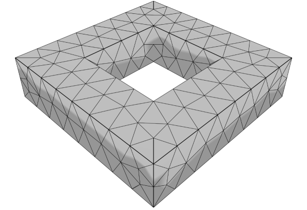
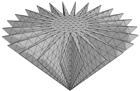
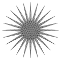
Figure 2: Triangulation of polyhedral boundaries used in numerical experiments. Left: A cuboid of dimension $1\mathrm{m}\times 1\mathrm{m}\times 0.25\mathrm{m}$ with a concentric cuboid hole of dimension $0.5\mathrm{m}\times 0.5\mathrm{m}\times 0.25\mathrm{m}$. Right: A pyramid of height $0.5\mathrm{m}$ and 24-pointed star base (bottom-right corner), whose vertices lie on two concentric circles of radius $1\mathrm{m}$ and $0.3\mathrm{m}$.

In order to examine the convergence of the Galerkin discretization scheme (16), we define the relative error

$$\mathrm{err}_{h}:=\dfrac{\left|{\left\lVert{\boldsymbol{u}_{h}}\right\rVert_{\sim,\operatorname{\mathbf{X}}_{\Gamma}}-\left\lVert{\boldsymbol{u}_{\mathrm{ref}}}\right\rVert_{\sim,\operatorname{\mathbf{X}}_{\Gamma}}}\right|}{\left\lVert{\boldsymbol{u}_{\mathrm{ref}}}\right\rVert_{\sim,\operatorname{\mathbf{X}}_{\Gamma}}},$$

where $\boldsymbol{u}_{\mathrm{ref}}$ is a reference solution to (16) computed with a very fine mesh, and the equivalent norm $\left\lVert{\cdot}\right\rVert_{\sim,\operatorname{\mathbf{X}}_{\Gamma}}$ on $\operatorname{\mathbf{X}}_{\Gamma}$ is defined for all $\boldsymbol{u}\in\operatorname{\mathbf{X}}_{\Gamma}$ as follows

$$\left\lVert{\boldsymbol{u}}\right\rVert^{2}_{\sim,\operatorname{\mathbf{X}}_{\Gamma}}:=\left\langle{\boldsymbol{u},S_{i\kappa}\overline{\boldsymbol{u}}}\right\rangle_{\times,\Gamma}.$$

By means of a triangle inequality, the relative error $\mathrm{err}_{h}$ exhibits the same convergence rate with that stated in Theorem 5.7.

Next, we examine the well-conditioning of the matrix system (25) by computing the condition number of the matrix $\operatorname{\mathbf{D}}^{-1}\operatorname{\mathbf{B}}$ for different meshwidth $h$. In addition, to investigate the performance of the proposed discretization with iterative solvers, the corresponding number of GMRES iterations required to solve $\eqref{eq:matrix_system}$ (with tolerance $\varepsilon_{0}=10^{-8}$) is also reported. Even though the bounded condition number of $\operatorname{\mathbf{D}}^{-1}\operatorname{\mathbf{B}}$ does not imply a fast convergence of GMRES solvers, it shows a good prediction in the numerical experiments below as well as in practical applications. The condition number and the corresponding GMRES iteration counts of the Galerkin discretization of the MFIE are then compared with those of the EFIE

(26) $$S_{\kappa}\boldsymbol{u}=\left({\dfrac{1}{2}Id+C_{\kappa}}\right)\left({\gamma_{D}^{+}\boldsymbol{e}^{in}}\right),$$

which is derived by taking the exterior tangential trace $\gamma_{D}^{+}$ of the Stratton-Chu representation formula (6) with $\sigma=\kappa$. The EFIE (26) is discretized using lowest-order Raviart-Thomas boundary elements for both the solution space and the test space, as investigated in [22].

6.1 Multiply-connected cuboid

We start with the scattering by a multiply-connected cuboid of dimension $1\mathrm{m}\times 1\mathrm{m}\times 0.25\mathrm{m}$ with a concentric cuboid hole of dimension $0.5\mathrm{m}\times 0.5\mathrm{m}\times 0.25\mathrm{m}$, see Figure 2 (left).

The reference solution $\boldsymbol{u}_{\mathrm{ref}}$ is computed with the boundary mesh $\Gamma_{h}$ characterized by the meshwidth $h=0.0125\mathrm{m}$. At each vertex of the boundary $\Gamma$, there are only three edges meeting, with opening angles $\varphi_{1},\varphi_{2}$ and $\varphi_{3}$ equal $\pi/2$ or $3\pi/2$. Thus, the regularity parameter $s^{\ast}=2\pi/(\varphi_{1}+\varphi_{2}+\varphi_{3})-\varepsilon>1/2$, see [22]. It means that the convergence rate, in this case, only depends on the regularity exponent $s$ of the solution, but not on $s^{\ast}$. More specifically, one can obtain the optimal convergence rate $\mathcal{O}(h^{1.5})$ for the Galerkin discretization (16) of the MFIE on this domain, provided that the continuous solution is sufficiently regular, i.e, $\boldsymbol{u}\in\operatorname{\mathbf{H}}^{s}_{\times}(\textup{div}_{\Gamma},\Gamma),s\geq 1$. Figure 3 (left) confirms this assertion.

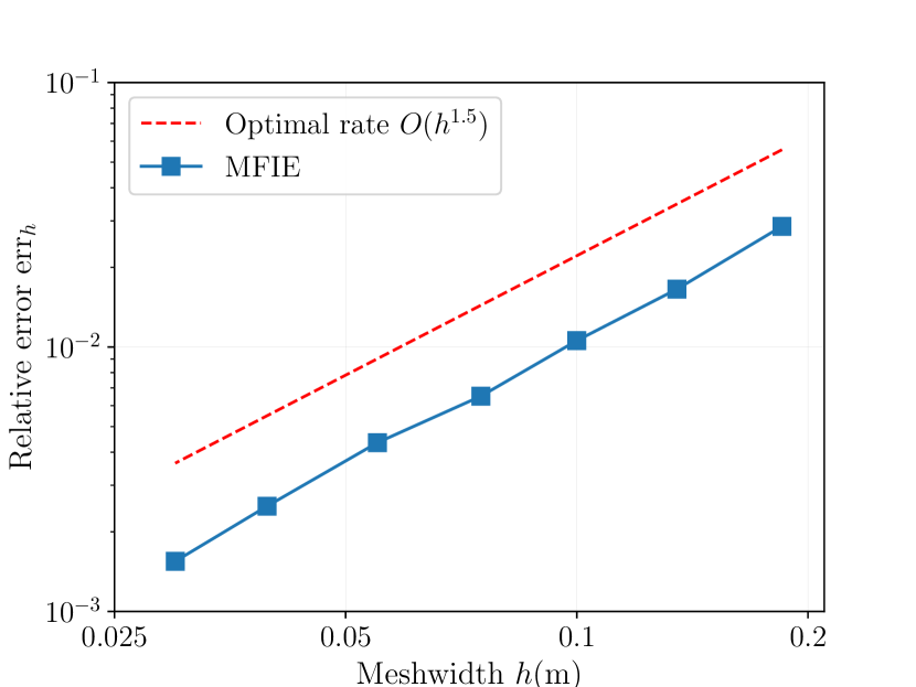
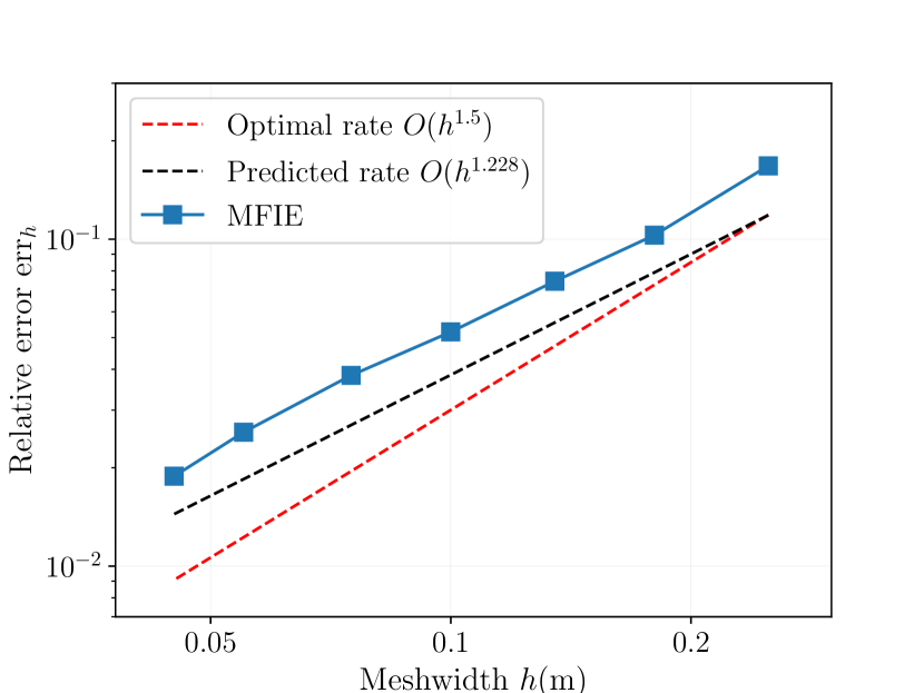
Figure 3: Relative error of numerical solutions to the MFIE with respect to meshwidth $h$. Left: A cuboid of dimension $\mathrm{1\mathrm{m}\times 1\mathrm{m}\times 0.25\mathrm{m}}$ with a concentric cuboid hole of dimension $\mathrm{0.5\mathrm{m}\times 0.5\mathrm{m}\times 0.25\mathrm{m}}$. The numerical solutions converge to the reference solution with an optimal rate. Right: A pyramid of height $0.5\mathrm{m}$ and a 24-pointed star base, whose vertices lie on two circles of radius $1\mathrm{m}$ and $0.3\mathrm{m}$. The numerical solutions exhibit a sub-optimal convergence rate due to the singularities of solution at the bottom vertex.

Figure 4 (left) depicts the conditioning properties of the Galerkin discretization of the EFIE and MFIE on the multiply-connected cuboid. Whereas the condition number of the Galerkin matrix of the EFIE and the corresponding number of GMRES iterations grow as $\mathcal{O}(h^{-2})$, those of the MFIE stay almost constant. This result confirms the well-conditioning of the Galerkin discretization (16) of the MFIE.

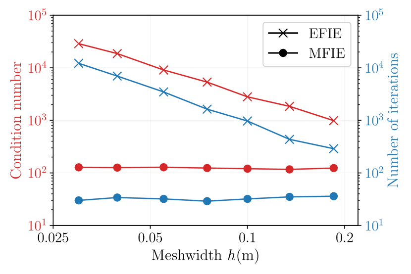
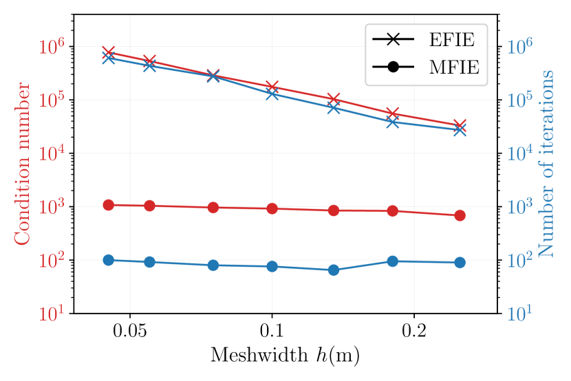
Figure 4: Condition number and corresponding number of GMRES iterations required to solve the linear systems produced by the Galerkin discretization of the EFIE and the MFIE. Left: A cuboid of dimension $\mathrm{1m\times 1m\times 0.25m}$ with a concentric hole of dimension $\mathrm{0.5m\times 0.5m\times 0.25m}$. Right: A pyramid of height $0.5\mathrm{m}$ and 24-pointed star base, whose vertices lie on two circles of radius $1\mathrm{m}$ and $0.3\mathrm{m}$. Whereas the condition number and the corresponding GMRES iteration counts of the EFIE grow when the meshwidth $h$ decreases, those of the MFIE stay almost constant.

6.2 Star-based pyramid

The second experiment concerns the scattering by a perfectly conducting pyramid with height $0.5\mathrm{m}$ and 24-pointed star base whose vertices lie on two circles of radius $1\mathrm{m}$ and $0.3\mathrm{m}$, see Figure 2 (right).

On a polyhedral boundary $\Gamma$, the regularity parameter $s^{\ast}$ can be determined by

$$s^{\ast}=\min_{v\in\Gamma}\dfrac{2\pi}{\left|{\partial\omega_{v}}\right|},$$

where $\omega_{v}$ is the domain on the unit sphere cut out by the tangent cone to $\Gamma$ at a vertex $v$ of $\Gamma$ (see [6, Theorem 8]). On the considered star-based pyramid, the boundary length of the curvilinear polygon $\omega_{v}$ reaches its maximum at the bottom vertex $v_{0}$ of the boundary $\Gamma$, at which 48 edges meet. Particularly, we can find $s^{\ast}\approx 0.228$. Hence, according to Theorem 5.7, only a sub-optimal convergence rate $\mathcal{O}(h^{1.228})$ can be expected on this domain. Figure 3 (right) confirms our convergence analysis. Here, the reference solution $\boldsymbol{u}_{\mathrm{ref}}$ is computed at the meshwidth $h=0.02\mathrm{m}$. Finally, Figure 4 (right) confirms again the well-conditioning property of the proposed Galerkin discretization scheme (16) for the MFIE.

7 Conclusions

We have provided rigorous numerical analysis of a Galerkin boundary element discretization of the magnetic field integral equation on Lipschitz polyhedra. The continuous variational problem has been shown to be uniquely solvable, provided that the wave number does not belong to the spectrum of the interior Maxwell’s problem. A Galerkin discretization of the variational formulation has been analyzed, which employs Raviart-Thomas boundary elements for the solution space and Buffa-Christiansen elements for the test space. The unique solvability and the well-conditioning of the discrete system have been proven, and the convergence rate of the discretization scheme has been investigated. Some numerical results have also been presented, corroborating the theoretical analysis as well as the effect of the singularities of Maxwell’s solutions on polyhedra to the convergence rate. The analyzed discretization scheme has been widely used in practical applications.

In future works, we shall investigate Galerkin discretization schemes for combined field integral equations and single source integral equations that employ the proposed discretization scheme for the double layer part.

References

- [1] A. Buffa, Hodge decompositions on the boundary of nonsmooth domains: the multi-connected case, Math. Models Methods Appl. Sci., 11 (2001), pp. 1491–1503.
- [2] A. Buffa and S. H. Christiansen, A dual finite element complex on the barycentric refinement, Math. Comput., 76 (2007), pp. 1743–1770.
- [3] A. Buffa and P. Ciarlet, On traces for functional spaces related to Maxwell’s equations Part I: An integration by parts formula in Lipschitz polyhedra, Math. Methods Appl. Sci., 24 (2001), pp. 9–30.
- [4] A. Buffa and P. Ciarlet, On traces for functional spaces related to Maxwell’s equations Part II: Hodge decompositions on the boundary of Lipschitz polyhedra and applications, Math. Methods Appl. Sci., 24 (2001), pp. 31–48.
- [5] A. Buffa, M. Costabel, and C. Schwab, Boundary element methods for Maxwell’s equations on non-smooth domains, Numer. Math., 92 (2002), pp. 679–710.
- [6] A. Buffa, M. Costabel, and D. Sheen, On traces for H(curl,) in Lipschitz domains, J. Math. Anal. Appl., 276 (2002), pp. 845–867.
- [7] A. Buffa and R. Hiptmair, Galerkin boundary element methods for electromagnetic scattering, in Lecture Notes in Computational Science and Engineering, vol. 31, Springer Berlin Heidelberg, 2003, pp. 83–124.
- [8] A. Buffa and R. Hiptmair, A coercive combined field integral equation for electromagnetic scattering, SIAM J. Numer. Anal., 42 (2005), pp. 621–640.
- [9] A. Buffa, R. Hiptmair, T. von Petersdorff, and C. Schwab, Boundary element methods for Maxwell transmission problems in Lipschitz domains, Numer. Math., 95 (2003), pp. 459–485.
- [10] M. Cessenat, Mathematical methods in electromagnetism, vol. 41 of Series on Advances in Mathematics for Applied Sciences, World Scientific, 1996.
- [11] S. H. Christiansen and J.-C. Nédélec, A preconditioner for the electric field integral equation based on Calderon formulas, SIAM J. Numer. Anal., 40 (2002), pp. 1100–1135.
- [12] P. G. Ciarlet, The finite element method for elliptic problems, vol. 40 of Classics in Applied Mathematics, Society for Industrial and Applied Mathematics, 2002.
- [13] X. Claeys and R. Hiptmair, Electromagnetic scattering at composite objects : a novel multi-trace boundary integral formulation, ESAIM: Math. Model. Numer. Anal., 46 (2012), pp. 1421–1445.
- [14] D. Colton and R. Kress, Inverse acoustic and electromagnetic scattering theory, vol. 93 of Applied Mathematical Sciences, Springer Berlin, first ed., 1992.
- [15] K. Cools, F. P. Andriulli, D. De Zutter, and E. Michielssen, Accurate and conforming mixed discretization of the MFIE, IEEE Antennas Wirel. Propag. Lett., 10 (2011), pp. 528–531.
- [16] K. Cools, F. P. Andriulli, F. Olyslager, and E. Michielssen, Time domain Calderón identities and their application to the integral equation analysis of scattering by PEC objects Part I: Preconditioning, IEEE Trans. Antennas Propag., 57 (2009), pp. 2352–2364.
- [17] M. Costabel and M. Dauge, Singularities of electromagnetic fields in polyhedral domains, Archive for Rational Mechanics and Analysis, 151 (2000), pp. 221–276.
- [18] C. P. Davis and K. F. Warnick, Error analysis of 2-D MoM for MFIE/EFIE/CFIE based on the circular cylinder, IEEE Trans. Antennas Propag., 53 (2005), pp. 321–331.
- [19] O. Ergul and L. Gurel, Improved testing of the magnetic-field integral equation, IEEE Microw. Wirel. Compon. Lett., 15 (2005), pp. 615–617.
- [20] P. Grisvard, Elliptic problems in nonsmooth domains, Pitman Publishing, 1985.
- [21] R. Hiptmair, Boundary element methods for eddy current computation, in Boundary element analysis, vol. 29 of Lecture Notes in Applied and Computational Mechanics, Springer Berlin Heidelberg, 2003, pp. 213–248.
- [22] R. Hiptmair and C. Schwab, Natural boundary element methods for the electric field integral equation on polyhedra, SIAM J. Numer. Anal., 40 (2003), pp. 66–86.
- [23] J. Kornprobst and T. F. Eibert, An accurate low-order discretization scheme for the identity operator in the magnetic field and combined field integral equations, IEEE Trans. Antennas Propag., 66 (2018), pp. 6146–6157.
- [24] J. Kornprobst and T. F. Eibert, Accuracy analysis of div-conforming hierarchical higher-order discretization schemes for the magnetic field integral equation, IEEE J. Multiscale Multiphysics Comput. Tech., 8 (2023), pp. 261–268.
- [25] V. C. Le and K. Cools, An operator preconditioned combined field integral equation for electromagnetic scattering, submitted for publication, (2023), https://doi.org/10.48550/arXiv.2309.02289.
- [26] V. C. Le, P. Cordel, F. P. Andriulli, and K. Cools, A stabilized time-domain combined field integral equation using the quasi-Helmholtz projectors, submitted for publication, (2023), https://doi.org/10.48550/arXiv.2312.06367.
- [27] V. C. Le, P. Cordel, F. P. Andriulli, and K. Cools, A Yukawa-Calderón time-domain combined field integral equation for electromagnetic scattering, in Proc. Int. Conf. Electromagn. Adv. Appl. (ICEAA), 2023.
- [28] A. Merlini, Y. Beghein, K. Cools, E. Michielssen, and F. P. Andriulli, Magnetic and combined field integral equations based on the quasi-Helmholtz projectors, IEEE Trans. Antennas Propag., 68 (2020), pp. 3834–3846.
- [29] J.-C. Nédélec, Acoustic and electromagnetic equations: Integral Representations for Harmonic Problems, vol. 144 of Applied Mathematical Sciences, Springer New York, 2001.
- [30] S. Rao, D. Wilton, and A. Glisson, Electromagnetic scattering by surfaces of arbitrary shape, IEEE Trans. Antennas Propag., AP-30 (1982), pp. 409–418.
- [31] P. A. Raviart and J. M. Thomas, A mixed finite element method for 2-nd order elliptic problems, in Lecture Notes in Mathematics, vol. 606, Springer Berlin Heidelberg, 1977, pp. 292–315.
- [32] J. M. Rius, E. Úbeda, and J. Parrón, On the testing of the magnetic field integral equation with RWG basis functions in method of moments, IEEE Trans. Antennas Propag., 49 (2001), pp. 1550–1553.
- [33] S. A. Sauter and C. Schwab, Boundary element methods, Springer Series in Computational Mathematics, Springer Berlin Heidelberg, 2011.
- [34] O. Steinbach and M. Windisch, Modified combined field integral equations for electromagnetic scattering, SIAM J. Numer. Anal., 47 (2009), pp. 1149–1167.