Bayesian Learning-driven Prototypical Contrastive Loss for Class-Incremental Learning

Abstract

The primary objective of methods in continual learning is to learn tasks in a sequential manner over time from a stream of data, while mitigating the detrimental phenomenon of catastrophic forgetting. In this paper, we focus on learning an optimal representation between previous class prototypes and newly encountered ones. We propose a prototypical network with a Bayesian learning-driven contrastive loss (BLCL) tailored specifically for class-incremental learning scenarios. Therefore, we introduce a contrastive loss that incorporates new classes into the latent representation by reducing the intra-class distance and increasing the inter-class distance. Our approach dynamically adapts the balance between the cross-entropy and contrastive loss functions with a Bayesian learning technique. Empirical evaluations conducted on both the CIFAR-10 dataset for image classification and images of a GNSS-based dataset for interference classification validate the efficacy of our method, showcasing its superiority over existing state-of-the-art approaches.

Index Terms—Continual Learning, Class-Incremental Learning, Representation Learning, Bayesian Learning, Contrastive Loss, Image Classification.

1 Introduction

Numerous practical vision applications necessitate the learning of new visual capabilities while maintaining high performance on existing ones. Examples include construction safety, employing reinforcement learning methodologies [25], or adapting to novel interference types in global navigation satellite system (GNSS) operations [39, 4, 41, 52]. The concept of continual learning denotes the capability to sequentially learn consecutive tasks without forgetting how to perform previously trained tasks. However, continual learning presents distinct challenges due to the tendency to lose information from previously learned tasks that may be relevant to the current task [25] – called catastrophic forgetting. This scenario commonly occurs when models are trained successively on multiple tasks. Recent methodologies try to circumvent catastrophic forgetting through various strategies. These include the utilization of feature extraction and fine-tuning adaptation techniques [32], leveraging off-policy learning and behavioral cloning from replay to enhance stability [45], and selectively decelerating learning on weights important for specific tasks [25]. Furthermore, literature states that the model size of the specialized components, i.e., shallow and deep layers, is important for new tasks [61]. Specifically, the learned data representation between preceding and novel tasks hold considerable importance [44]. This serves as a motivation for our focus on refining the architecture of specialized blocks and enhancing dynamic representations for continual learning, as depicted in Figure 1.

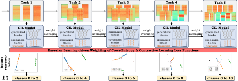
Figure 1: Overview of our continual learning method with Bayesian weighting.

A related yet distinct task is contrastive learning, which pairs positive and negative instances with corresponding anchors to enrich training [8, 40]. While continual learning with contrastive techniques are prevalent in semantic tasks [22], contrastive learning’s application in continual learning for image classification tasks is limited [6]. This limitation arises from the potential decrease in diversity of negative samples, affecting the task-specific loss, and the likelihood of the regularizer may hinder learning of new distinctive representations [7]. Recognizing the importance of weighting both the classification and contrastive loss functions to achieve a balance between previous and new tasks, our approach proposes a Bayesian learning-driven strategy [23, 24]. A notable challenge arises from the inconsistency of negative samples between classification and representation learning tasks [34]. A Bayesian framework facilitates the inference of probabilities for contrastive model samples, eliminating the necessity for computationally intensive hyperparameter tuning searches [19].

The primary objective of this work is to propose a continual learning approach capable of adapting to novel classes. Our contributions are outlined as follows: (1) We introduce the continual learning method BLCL, which is founded on the ResNet [20] architecture, incorporating dynamic specialized components tailored for each task. (2) We contribute a novel loss function that combines the cross-entropy (CE) loss with a contrastive learning loss, incorporating class embedding distances in a prototypical manner [48]. (3) We introduce a Bayesian learning-driven [23, 24] dynamic weighting mechanism for both loss functions. (4) Our evaluations conducted on the CIFAR-10 [28] and a GNSS [39] dataset demonstrate that BLCL yields an enhanced feature representation, resulting in improved classification accuracy for image-related tasks.

The remainder of this paper is organized as follows. Section 2 provides a comprehensive overview of the existing literature for continual learning. In Section 3, we propose our methodology, incorporating a Bayesian learning-driven contrastive loss. We present experiments in Section 4. Section 5 summarizes evaluation results, followed by the concluding remarks in Section 6.

2 Related Work

Initially, we present related work concerning continual learning (see Section 2.1), which serves as the foundation of state-of-the-art methodologies utilized in our experiments. Subsequently, in Section 2.2, we summarize Bayesian contrastive learning techniques.

2.1 Continual/Class-Incremental Learning

Class-incremental learning (CIL) aims to continuously develop a comprehensive classifier for all encountered classes. The primary challenge in CIL lies in catastrophic forgetting, where direct optimization of the network with new classes leads to the erasure of knowledge pertaining to former tasks, thereby resulting in irreversible performance degradation. The objective is to effectively mitigate catastrophic forgetting [60]. Conventional ML models address CIL through dual tasks by updating only the model with a single new stage [31, 29, 10]. Feature extraction methods [14] maintain the set of shared network parameters ($\Theta_{s}$) and task-specific parameters for previously learned tasks ($\Theta_{o}$) unchanged. Here, only the outputs of one or more layers serve as features for the new task, employing randomly initialized task-specific parameters ($\Theta_{n}$). In finetune [17] methods, $\Theta_{o}$ remains fixed, while $\Theta_{s}$ and $\Theta_{n}$ are optimized for the new task. Kirkpatrick et al. [25] proposed elastic weight consolidation (EWC), which selectively decelerates learning on weights crucial for previous tasks. The method learning without forgetting (LwF), introduced by Li et al. [32], employs solely new task data to train the network while retaining the original capabilities. Rolnick et al. [45] proposed CLEAR (continual learning with experience and replay) for multi-task reinforcement learning, leveraging off-policy learning and behavioral cloning from replay to enhance stability, as well as on-policy learning to preserve plasticity. Rebuffi et al. [44] introduced iCaRL (incremental classifier and representation learning), which learns such that only the training data for a small number of classes needs to be present concurrently, allowing for progressive addition of new classes. iCaRL combines a classification loss with a distillation loss to replicate the scores stored in the previous step. Replay, introduced by Ratcliff et al. [43], investigates manipulations of the network within a multilayer model and various variants thereof.

Conventional CIL methods typically prioritize representative exemplars from previous classes to mitigate forgetting. However, recent investigations indicate that preserving models from history can significantly enhance performance. Certain applications necessitate memory-efficient architectures. However, state-of-the-art CIL methods are not compared with regard to their memory budget. The memory-efficient expandable model (MEMO) [61] addresses this gap by simultaneously considering accuracy and memory size, analyzing the impact of different network layers. Zhou et al. [61] discovered that shallow and deep layers exhibit distinct characteristics in the context of CIL. MEMO extends specialized layers based on shared generalized representations, efficiently extracting diverse representations at modest cost while maintaining representative exemplars. Given that MEMO achieves superior accuracies on state-of-the-art datasets, we adopt MEMO as our methodological baseline. However, we observe that results can be further enhanced by incorporating dynamic specialized blocks (the last layers for which the weights are averaged with the previous task). In our experiments, we compare the performance of finetune, EWC, LwF, iCarl, Replay, and MEMO. Further CIL methods are reinforced memory management (RMM) [35], gradient episodic memory (GEM) [36], dynamically expandable representation (DER) [58], dynamic token expansion (DyTox) [16], learning to prompt (L2P) [54], pooled outputs distillation (PODNet) [15], weight aligning (WA) [59], and bias correction (BiC) [56]. For a comprehensive overview of methodologies, refer to [60, 30, 38, 53, 37, 3, 50].

2.2 Bayesian Contrastive Learning

Contrastive learning establishes pairs of positive and negative instances along corresponding anchors to enhance training [8]. This approach has found extensive application across various domains including multi-modal learning [55, 42, 21], domain adaptation [49], and semantic learning tasks [22, 46]. The contrastive learning paradigm has been extended to triplet learning [40, 47], which utilizes a positive sample, and quadruplet learning [39, 9], which employs a similar sample. The main focus within this field resolves around the optimal selection of pairs to augment training. However, the primary focus of our study resides in determining the optimal weighting between classification and contrastive loss functions.

Cha et al. [6] demonstrated that representations learned contrastively exhibit greater robustness against catastrophic forgetting compared to those trained using the CE loss. Their approach integrates an asymmetric variant of supervised contrastive loss, mitigating model overfitting to a limited number of previous task samples by employing a dynamic architecture. Similarly, Sy-CON [7] also integrates symmetric contrastive loss. Hasanzadeh et al. [19] utilize distributional representations to provide uncertainty estimates in downstream graph analytic tasks. Lin et al. [33] employ Monte Carlo dropout on skeleton data for action recognition, generating pairwise samples for model robustness. Liu et al. [34] introduced a Bayesian contrastive loss (BCL) to mitigate false negatives and mine hard negative samples, aligning the semantics of negative samples across tasks. Instead, our approach leverages Bayesian learning as proposed by Kendall et al. [23, 24] for weighting the CE and contrastive loss functions.

3 Methodology

This section provides a detailed description of our methodology. In Section 3.1, we mathematically formulate the problem of CIL. Subsequently, in Section 3.2, we provide an overview of our proposed method. We introduce a contrastive loss formulation and Bayesian learning-driven weighting strategy in Section 3.3, and we describe data augmentation techniques in Section 3.4.

3.1 Problem Formulation

Let us consider a sequence of $T$ training tasks denoted as $\{\mathcal{D}^{1},\mathcal{D}^{2},\cdots,\mathcal{D}^{T}\}$, where each $\mathcal{D}^{t}=\{(x_{i}^{t},y_{i}^{t})\}_{i=1}^{n_{t}}$ represents the $t$-th incremental step containing $n_{t}$ training instances of images. $x_{i}^{t}$ signifies a sample belonging to class $y_{i}\in Y_{t}$, with $Y_{t}$ representing the label space of task $t$. During the training of task $t$, only data from $\mathcal{D}^{t}$ is available. The objective is to continuously develop a classification model encompassing all classes encountered thus far. Subsequent to each task, the model is evaluated across all observed classes $\mathcal{Y}_{t}=Y_{1}\cup\cdots\cup Y_{t}$ [60, 44]. Typically, classes do not overlap across different tasks. However, in certain scenarios, previously encountered classes may reappear in subsequent tasks, constituting what is termed as blurry CIL [57, 27, 1, 2]. For the purpose of this paper, it is noted that the classes are overlapping as we have a fixed number of representative instances from the previous task classes, so-called exemplars.

3.2 Method Overview

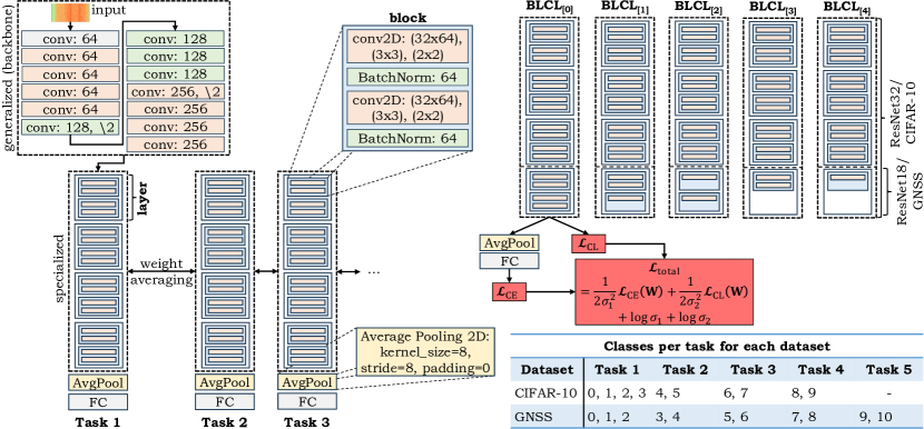
Figure 2: Overview of our Bayesian learning-driven continual learning architecture (BLCL). After the generalized component of ResNet [20], i.e., ResNet18 or ResNet32, follow up to eight blocks for the CIFAR-10 [28] dataset and two blocks for the GNSS [39] dataset. After each task the weights are averaged with the weights of the previous tasks. We propose a dynamic architecture with a different number of blocks and convolutional layers, indicated by $\text{BLCL}_{[*]}$. After the fully connected (FC) layer, follows a cross-entropy (CE) loss in combination with a Bayesian learning-driven weighting of the contrastive loss (CL).

Our methodology is outlined in Figure 2, designated as BLCL. It leverages the MEMO [61] architecture, initially pre-trained on ImageNet [12]. The ResNet model, proposed by He et al. [20], specifically ResNet18 or ResNet32, comprises both generalized and specialized components. The generalized component extracts features from the image dataset, featuring 13 convolutional layers, and is succeeded by one or more (up to four) additional layers. The specialized component contains of blocks, which weights are averaged with the weights from the previous task. These specialized layers contain different numbers of layers $l$, adapted to the dataset at hand, are denoted as $\text{BLCL}_{l}$, where each layer comprises two blocks, each containing two convolutional layers and two batch normalizations. The output dimension of the convolutional layers is set to 512. Subsequently, employ average pooling and a fully connected layer, we train utilizing the CE loss $\mathcal{L}_{\text{CE}}$. The training process involves freezing the specialized component from previous tasks while updating the generalized and specialized component with classes pertinent to the specific tasks. Moreover, we average the weights of the specialized component from previous tasks. To maintain adaptability to varying complexities of new classes across tasks, we dynamically adjust each task’s layer structure, denoted as $\text{BLCL}_{l[s]}$ (as depicted in the top right of Figure 2). This adaptation involves the removal of either one convolutional layer or an entire block from the specialized model’s layer configuration, catering to the evolving requirements of each task.

3.3 Loss Functions

The lower-level representation of the CIL model is continuously adapted with the addition of each new class, thereby potentially undergoing significant changes. The primary objective is to incrementally enhance class prototypes, thereby reducing intra-class distances while simultaneously increasing inter-class distances. To facilitate this objective, we introduce a contrastive loss term, denoted as $\mathcal{L}_{\text{CL}}$. Achieving an optimal balance between the CE and CL loss functions is crucial. Hence, we propose an automated weighting mechanism utilizing Bayesian learning techniques.

Contrastive Loss.

Pairwise learning is characterized by the utilization of pairs featuring distinct labels, serving to enrich the training process by enforcing a margin between pairs of images belonging to different identities. Consequently, the feature embedding for a specific label lives on a manifold while ensuring sufficient discriminability, i.e., distance, from other identities [40, 13]. CL, on the other hand, is a methodology aimed at training models to learn representations by maximizing the distance between positive pairs and minimizing the distance between negative pairs within a latent space. We define feature embeddings $f(\mathbf{X})\in\mathbb{R}^{q\times h}$ to map the image input into a feature space $\mathbb{R}^{q\times h}$, where $f$ represents the output of the last convolutional layer with a size of 512 from the specialized model, and $q\times h$ denotes the dimensionality of the layer output. Consequently, we define an anchor sample $\mathbf{X}_{i}^{a}$ corresponding to a specific label, a positive sample $\mathbf{X}_{i}^{p}$ from the same label, and a negative sample $\mathbf{X}_{i}^{n}$ drawn from a different label. For all training samples $\big{(}f(\mathbf{X}_{i}^{a}),f(\mathbf{X}_{i}^{p}),f(\mathbf{X}_{i}^{n})\big{)}\in\Phi$, our objective is to fulfill the following inequality:

$$d\big{(}f(\mathbf{X}_{i}^{a}),f(\mathbf{X}_{i}^{p})\big{)}+\alpha<d\big{(}f(\mathbf{X}_{i}^{a}),f(\mathbf{X}_{i}^{n})\big{)},$$ (1)

where $d$ is a distance function, specifically the cosine distance $\text{CD}(\mathbf{x}_{1},\mathbf{x}_{2})=1-\frac{\mathbf{x}_{1}\cdot\mathbf{x}_{2}}{||\mathbf{x}_{1}||\cdot||\mathbf{x}_{2}||}$ computed between two non-zero vectors $\mathbf{x}_{1},\mathbf{x}_{2}\in\mathbb{R}^{n}$ of size $n$, $\alpha=1$ denotes a margin differentiating positive and negative pairs, and $\Phi$ is the set of all possible pairs within the training dataset, where $N$ is the number of pairs. For each batch of size $bs$, we select all conceivable pairs and increase the batch size to $\frac{bs(bs+1)}{2}$.

Bayesian Learning.

Typically, naïve methods employ a weighted combination of both loss functions to compute the total loss, denoted as $\mathcal{L}_{\text{total}}=w_{1}\mathcal{L}_{\text{CE}}+w_{2}\mathcal{L}_{\text{CL}}$. However, the model performance is extremely sensitive to the selection of weights $w_{i}$. In our approach, we adopt a strategy wherein we concurrently optimize both objectives using homoscedastic task uncertainty, as defined by Kendall et al. [23, 24]. This homoscedastic uncertainty pertains to the task-dependent aleatoric uncertainty, which remains invariant across input data but varies across distinct tasks [26]. Let $\text{f}^{\mathbf{W}}(\mathbf{X})$ denote the output of a neural network with weights $\mathbf{W}$ on input $\mathbf{X}$. In scenarios involving multiple model outputs, we factorize over the outputs

$$p\big{(}\mathbf{y}_{1},\ldots,\mathbf{y}_{K}|\text{f}^{\mathbf{W}}(\mathbf{X})\big{)}=p\big{(}\mathbf{y}_{1}|\text{f}^{\mathbf{W}}(\mathbf{X})\big{)}\ldots p\big{(}\mathbf{y}_{K}|\text{f}^{\mathbf{W}}(\mathbf{X})\big{)},$$ (2)

with $K$ model outputs $\mathbf{y}_{1},\ldots,\mathbf{y}_{K}$ [24]. In a classification task, we sample from a probability vector from a scaled softmax function’s output $p\big{(}\mathbf{y}|\text{f}^{\mathbf{W}}(\mathbf{X}),\sigma\big{)}=\text{softmax}\big{(}\frac{1}{\sigma^{2}}\text{f}^{\mathbf{W}}(\mathbf{X})\big{)}$. The log likelihood is then defined as

$$\log p\big{(}\mathbf{y}=c|\text{f}^{\mathbf{W}}(\mathbf{X})\big{)}=\frac{1}{\sigma^{2}}\text{f}_{c}^{\mathbf{W}}(\mathbf{X})-\log\sum_{c^{\prime}}\exp\big{(}\frac{1}{\sigma^{2}}\text{f}_{c}^{\mathbf{W}}(\mathbf{X})\big{)},$$ (3)

where $\text{f}_{c}^{\mathbf{W}}(\mathbf{X})$ is the $c$-th element of $\text{f}^{\mathbf{W}}(\mathbf{X})$. In a regression task, we maximize the log likelihood of the model, written as

$$\log p\big{(}\mathbf{y}|\text{f}^{\mathbf{W}}(\mathbf{X})\big{)}\propto-\frac{1}{2\sigma^{2}}||\mathbf{y}-\text{f}^{\mathbf{W}}(\mathbf{X})||^{2}-\log\sigma,$$ (4)

for a Gaussian likelihood $p\big{(}\mathbf{y}|\text{f}^{\mathbf{W}}(\mathbf{X})\big{)}=\mathcal{N}\big{(}\text{f}^{\mathbf{W}}(\mathbf{X}),\sigma^{2}\big{)}$, where $\sigma$ is the model’s observation noise parameter [24]. In our case, our model output is composed of two vectors, a discrete output $\mathbf{y}_{1}$ for the CE loss and continuous output $\mathbf{y}_{2}$ for the CL loss, which leads to the total minimization objective:

$$\begin{split}&\mathcal{L}(\mathbf{W},\sigma_{1},\sigma_{2})=-\log p\big{(}\mathbf{y}_{1}=c,\mathbf{y}_{2}|\text{f}^{\mathbf{W}}(\mathbf{X})\big{)}\\ &=-\text{softmax}\big{(}\mathbf{y}_{1}=c;\text{f}^{\mathbf{W}}(\mathbf{X}),\sigma_{1}\big{)}\cdot\log\mathcal{N}\big{(}\mathbf{y}_{2};\text{f}^{\mathbf{W}}(\mathbf{X}),\sigma_{2}^{2}\big{)}\\ &=-\log p\big{(}\mathbf{y}_{1}=c|\text{f}^{\mathbf{W}}(\mathbf{X}),\sigma_{1}\big{)}+\\ &+\frac{1}{2\sigma_{2}^{2}}||\mathbf{y}_{2}-\text{f}^{\mathbf{W}}(\mathbf{X})||^{2}+\log\sigma_{2}\\ &\approx\frac{1}{2\sigma_{1}^{2}}\mathcal{L}_{\text{CE}}(\mathbf{W})+\frac{1}{2\sigma_{2}^{2}}\mathcal{L}_{\text{CL}}(\mathbf{W})+\log\sigma_{1}+\log\sigma_{2}.\end{split}$$ (5)

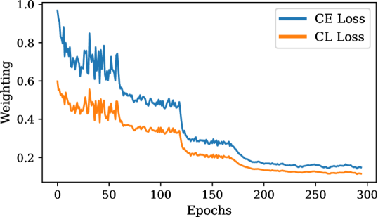
Figure 3: Weighting of the CE and CL loss functions on the CIFAR-10 dataset.

The final objective is to minimize Equation 5 with respect to $\sigma_{1}$ and $\sigma_{2}$, thereby learning the relative weights of the losses $\mathcal{L}_{1}(\mathbf{W})$ and $\mathcal{L}_{2}(\mathbf{W})$ in an adaptive manner [23, 24]. Figure 3 provides an illustrative demonstration of the weighting mechanism applied to both loss functions for the first task. As $\sigma_{1}$, respectively $\sigma_{2}$, the noise parameters associated with variable $\mathbf{y}_{1}$, respectively $\mathbf{y}_{2}$, increase, the weight assigned to $\mathcal{L}_{\text{CE}}$, respectively $\mathcal{L}_{\text{CL}}$, diminishes. Such an adjustment serves as a regularizer for the noise term. This trend is observable at the early period of each task (in Figure 3 for the first task), as new classes introduce more noise, and hence, the weighting of both loss functions decreases. In general, both loss functions have converged after 200 epochs.

3.4 Data Augmentation

Due to the potential for highly unbalanced training dataset, such as the interfered classes within the GNSS dataset, we address this issue by balancing each class through data augmentation techniques. Specifically, we augment the data to ensure a uniform distribution of 1,000 samples per class. We employ techniques provided by torchvision.transforms, including color jittering with a brightness value of 0.5 and a hue value of 0.3, Gaussian blur with a kernel size of $(5,9)$ and sigma values of $(0.1,5.0)$, random adjustments of sharpness with a sharpness factor of 2, and random horizontal and vertical flipping with a probability of 0.4. Values are chosen after a hyperparameter search.

4 Experiments

For fair comparability, we conduct experiments on two distinct image datasets: the CIFAR-10 dataset (see Section 4.1) and a GNSS-based dataset (see Section 4.2). Consequently, we encounter a diverse array of applications pertinent to continual learning, specifically within the realm of image classification tasks.

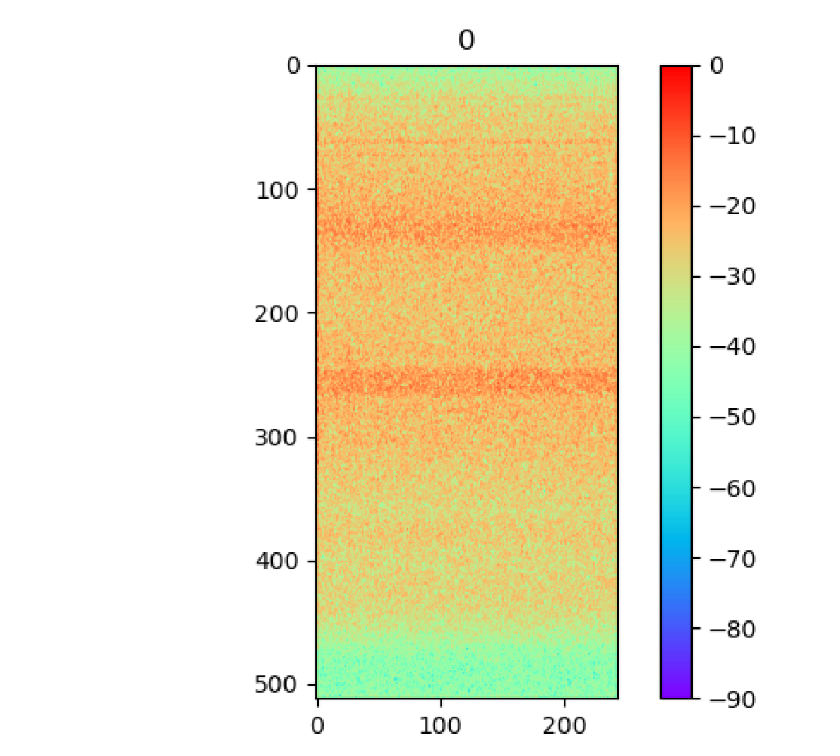
(a) 0.

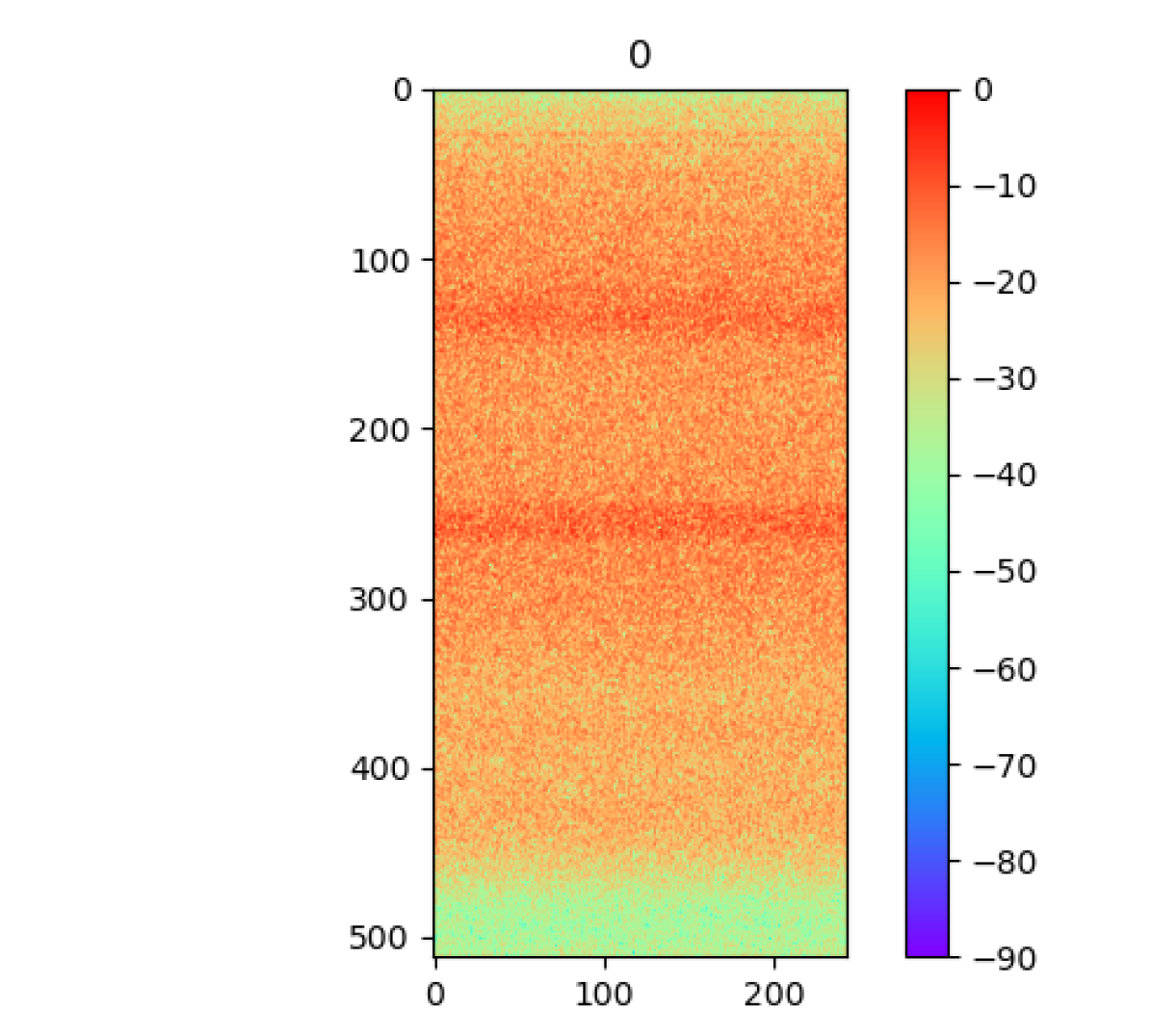
(b) 1.

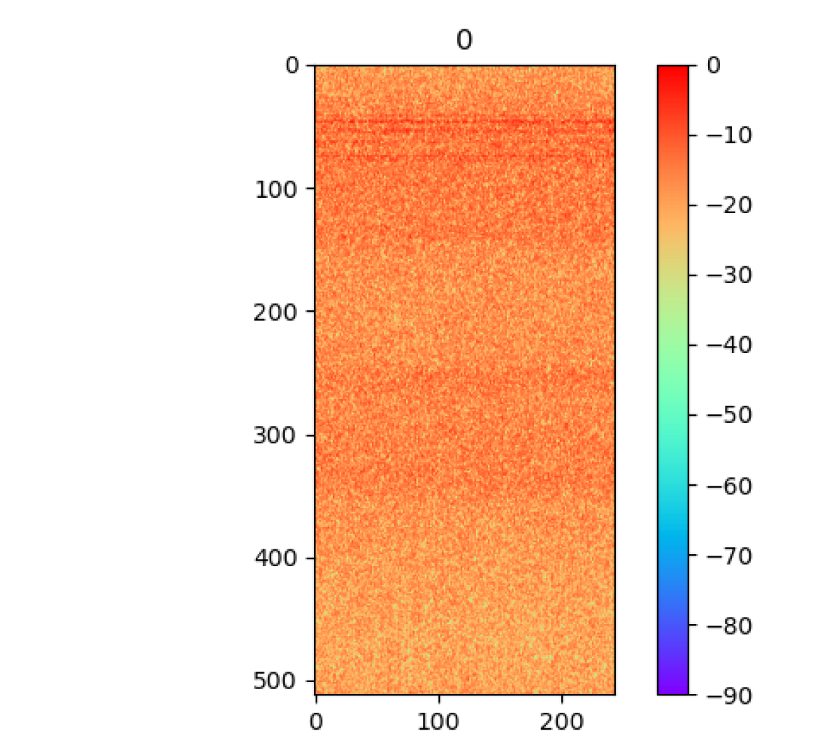
(c) 2.

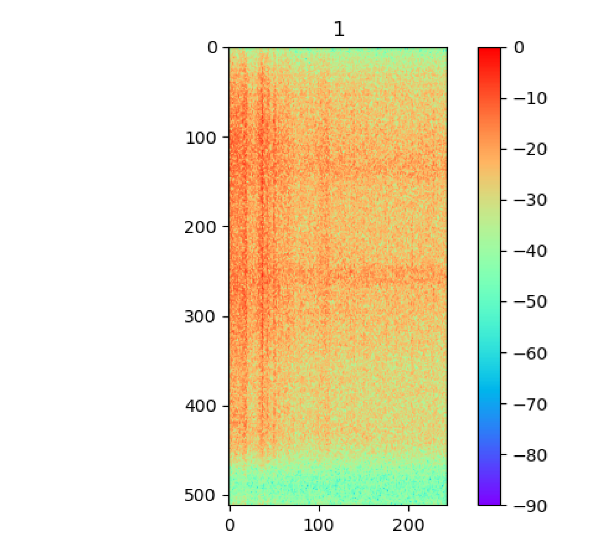
(d) 3.

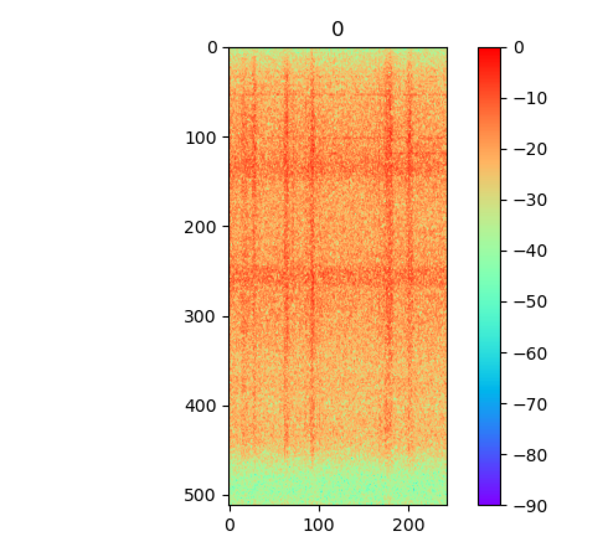
(e) 4.

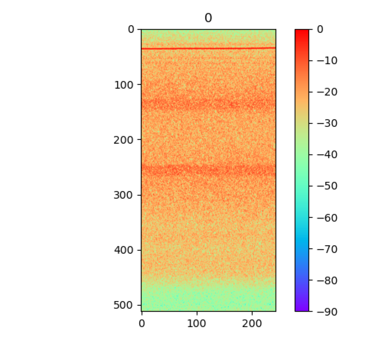
(f) 5.

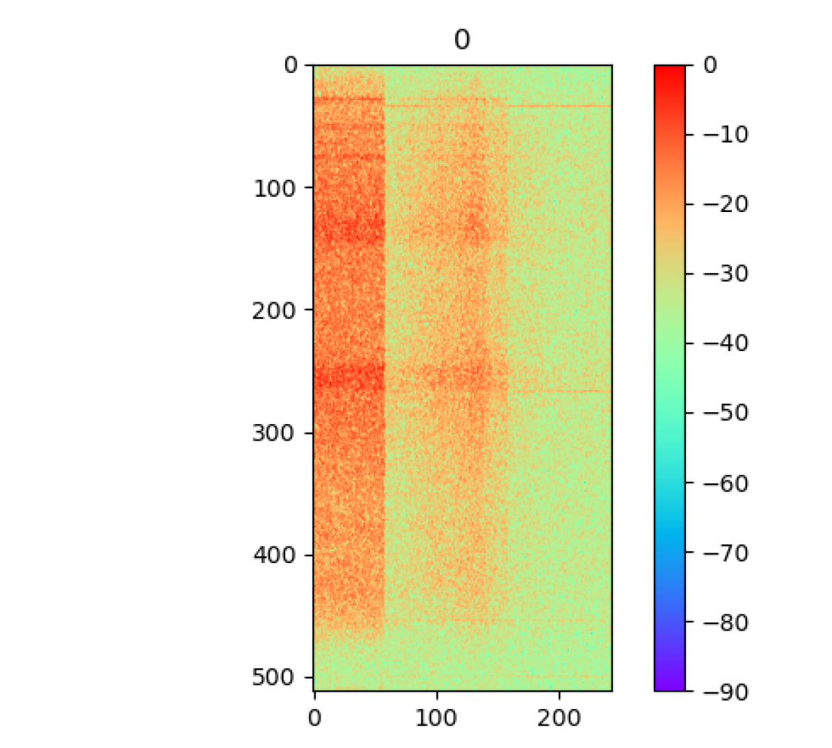
(g) 6.

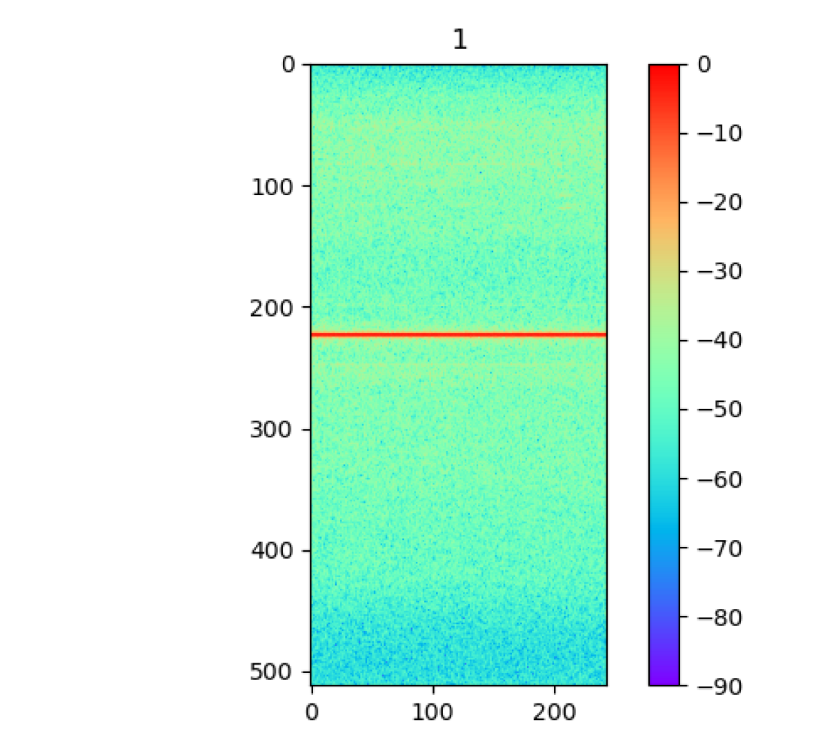
(h) 7.

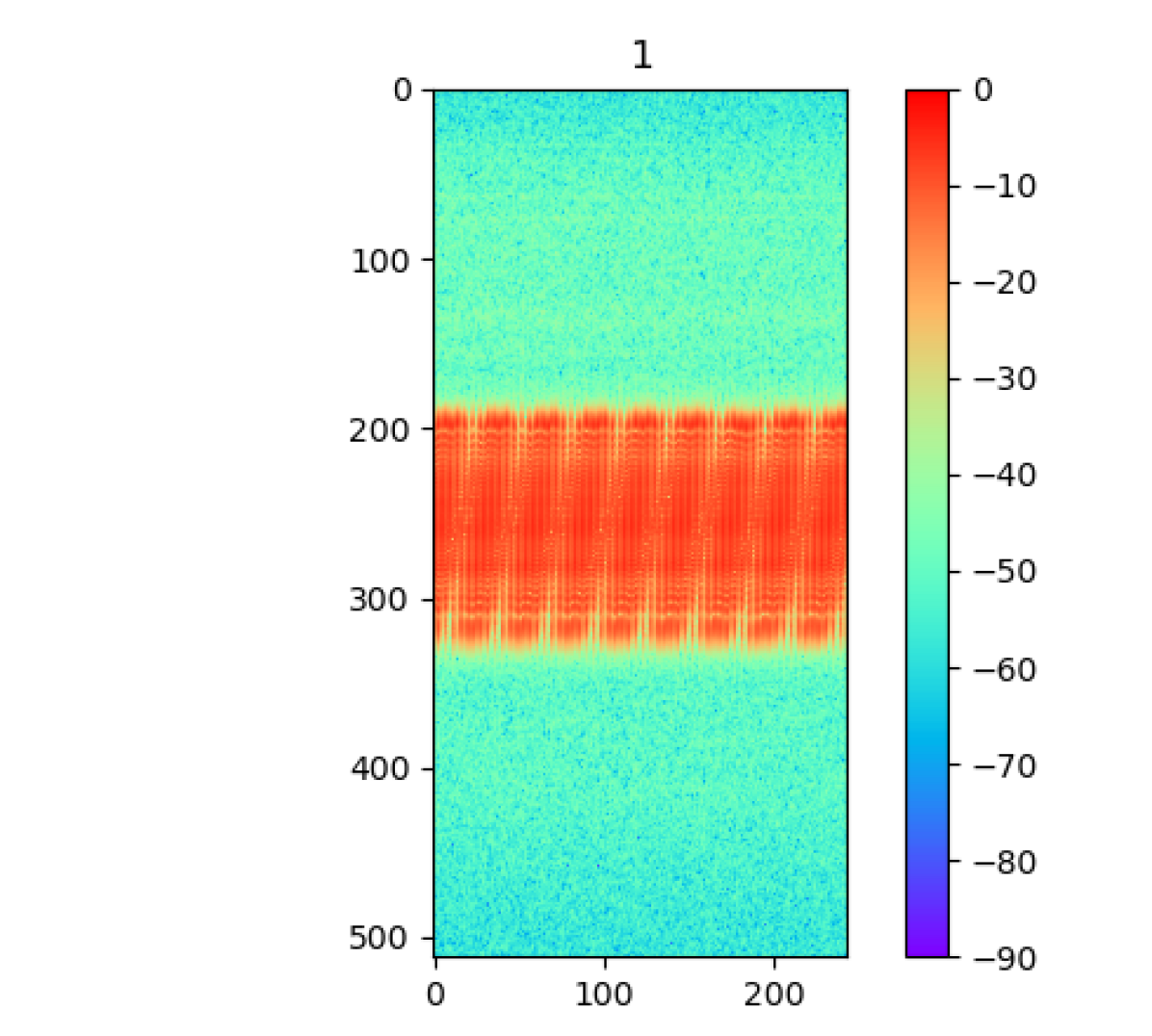
(i) 8.

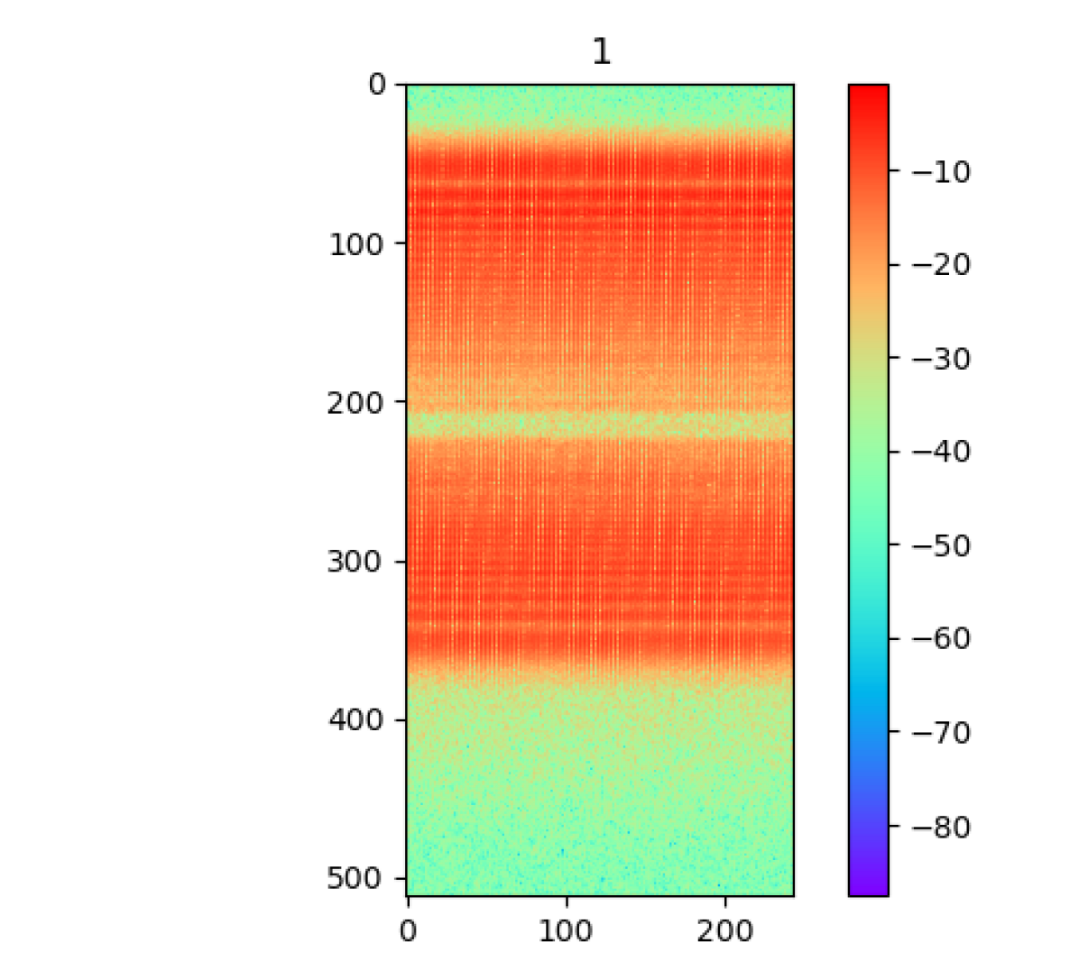
(j) 9.

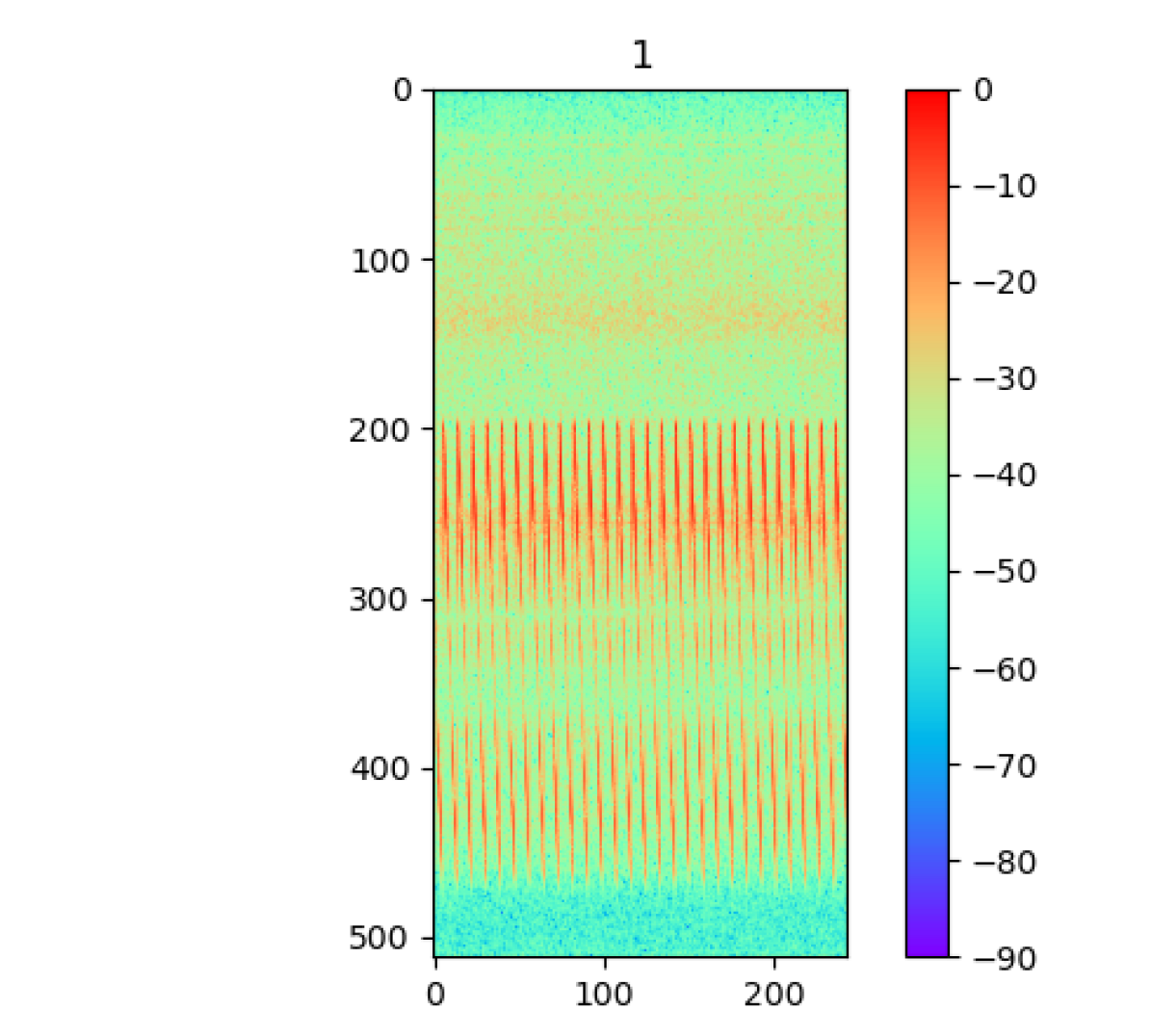
(k) 10.

Figure 4: Exemplary spectrogram samples without interference (classes 0 to 2) and with interference (classes 3 to 10) between intensity [0, -90] with logarithmic scale. The x-axis shows the time in ms. The y-axis shows the frequency in MHz.

4.1 Image Classification: CIFAR-10

The CIFAR-10 [28] dataset consists of 60,000 colour images of size $32\times 32$. The goal is to classify 10 distinct classes (i.e., airplane, automobile, bird, cat, deer, dog, etc.), with 6,000 images per class. The dataset is split into 50,000 training and 10,000 test images. We train four tasks: task 1 consists of the classes 0, 1, 2, and 3, task 2 consists of the classes 4 and 5, task 3 consists of the classes 6 and 7, and task 4 consists of the classes 8 and 9.

4.2 Interference Classification from GNSS Snapshots

The GNSS-based dataset, proposed by Ott et al. [39], contains short, wideband snapshots in both E1 and E6 GNSS bands. The dataset was captured at a bridge over a motorway. The setup records 20 ms raw IQ (in-phase and quadrature-phase) snapshots triggered from the energy with a sample rate of 62.5 MHz, an analog bandwidth of 50 MHz and an 8 bit bit-width. Further technical details can be found in [4]. Figure 4 shows exemplary snapshots of the spectrogram. Manual labeling of these snapshots has resulted in 11 classes: Classes 0 to 2 represent samples with no interferences, distinguished by variations in background intensity, while classes 3 to 10 contain different interferences such as pulsed, noise, tone, and multitone. For instance, Figure 4 showcases a snapshot containing a potential chirp jammer type. The dataset’s imbalance of 197,574 samples for non-interference classes and between 9 to 79 samples per interference class, emphasizing the under-representation of positive class labels. The goal is to adapt to new interference types with continual learning. The challenge lies in adapting to positive class labels with only a limited number of samples available. We partition the dataset into a 64% training set, 16% validation set, and a 20% test set split (balanced over the classes). We train five tasks: task 1 consists of the classes 0, 1, and 2, task 2 consists of the classes 3 and 4, task 3 consists of the classes 5 and 6, task 4 consists of the classes 7 and 8, and task 5 consists of the classes 9 and 10.

5 Evaluation

All experiments are conducted utilizing Nvidia Tesla V100-SXM2 GPUs with 32 GB VRAM, equipped with Core Xeon CPUs and 192 GB RAM. We use the vanilla Adam optimizer with a learning rate set to $0.1$, a decay rate of $0.1$, a batch size of 128, and train each task for 300 epochs. Initially, we present the results obtained through our BLCL approach, in comparison with state-of-the-art methods, on both the CIFAR-10 and the GNSS datasets. Subsequently, we conduct an analysis involving confusion matrices, model embeddings, cluster analysis, and parameter counts. Throughout, we provide the accuracy achieved after each task, the average accuracy over all tasks ($\overline{\text{Acc}.}$), as well as the F1-score and F2-score.

Table 1: Evaluation results for baseline methods, decreased blocks of model architectures, and our Bayesian-driven (B) contrastive loss functions on the CIFAR-10 [28] dataset. We indicate the weighting with (w/) and without (w/o) averaging. Underlined is the best baseline method and bold is the best method in total.

	Loss/	Task 1	Task 2	Task 3	Task 4	Final
Method	Weighting	Acc.	Acc.	Acc.	Acc.	$\overline{\mathbf{Acc.}}$	F1	F2
Finetune	CE	95.20	32.08	24.80	19.80	43.22	0.067	0.110
EWC [25]		95.20	54.30	47.39	36.10	58.24	0.303	0.324
LwF [32]		95.48	63.55	62.80	56.89	69.68	0.556	0.557
iCarl [44]		95.35	81.85	80.12	79.57	84.47	0.792	0.791
Replay [43]		95.35	78.95	76.69	76.72	81.93	0.766	0.764
MEMO [61], w/o	CE	96.00	80.68	80.79	81.68	84.78	0.810	0.812
$\text{BLCL}_{4[0,0,0,0]}$, w/	CE	96.00	80.68	79.56	77.89	83.53	0.776	0.776
$\text{BLCL}_{6[0,0,0,0]}$, w/o	CE	96.00	80.77	80.78	81.03	84.64	0.803	0.805
$\text{BLCL}_{8[0,0,0,0]}$, w/o	CE	95.55	81.67	80.95	81.91	85.02	0.813	0.815
$\text{BLCL}_{8[1,1,1,1]}$, w/o	CE	94.25	82.57	80.58	81.76	84.79	0.812	0.813
$\text{BLCL}_{8[2,2,2,2]}$, w/o	CE	94.22	82.53	80.28	81.83	84.97	0.814	0.814
$\text{BLCL}_{8[3,3,3,3]}$, w/o	CE	94.80	83.10	80.16	81.64	84.93	0.812	0.812
$\text{BLCL}_{8[4,4,4,4]}$, w/o	CE	94.38	83.37	80.08	81.31	84.79	0.809	0.809
$\text{BLCL}_{8[0,1,2,3]}$, w/o	CE	94.00	82.73	80.38	80.85	84.74	0.804	0.804
$\text{BLCL}_{8[0,0,3,4]}$, w/o	CE	94.00	82.83	80.91	81.58	84.83	0.811	0.812
$\text{BLCL}_{8[2,2,3,2]}$, w/o	CE	94.22	82.53	80.04	81.03	84.45	0.806	0.806
$\text{BLCL}_{8[3,3,2,3]}$, w/o	CE	94.80	83.10	79.15	81.76	84.70	0.813	0.813
$\text{BLCL}_{8[0,0,3,3]}$, w/o	CE	94.00	82.83	80.91	82.11	84.96	0.811	0.813
$\text{BLCL}_{8[0,0,3,3]}$, w/o	CE, 0.9, CL	95.15	78.85	78.89	78.71	82.90	0.778	0.780
$\text{BLCL}_{8[0,0,3,3]}$, w/o	CE, B, CL	95.28	83.58	83.04	83.10	85.92	0.814	0.814
$\text{BLCL}_{8[1,2,3,4]}$, w/o	CE	94.25	83.15	80.69	82.34	85.11	0.819	0.820
$\text{BLCL}_{8[1,2,3,4]}$, w/o	CE, 0.9, CL	95.82	80.13	80.36	80.73	84.26	0.800	0.802
$\text{BLCL}_{8[1,2,3,4]}$, w/o	CE, B, CL	95.55	83.92	82.85	81.88	86.05	0.815	0.816
$\text{BLCL}_{8[1,1,1,2]}$, w/o	CE	94.25	82.57	80.58	81.44	84.71	0.810	0.810
$\text{BLCL}_{8[1,1,1,2]}$, w/o	CE, 0.9, CL	95.85	79.93	79.95	80.87	84.61	0.802	0.804
$\text{BLCL}_{8[1,1,1,2]}$, w/o	CE, B, CL	95.58	84.50	82.55	83.62	86.56	0.833	0.834
$\text{BLCL}_{8[1,1,2,2]}$, w/o	CE	94.25	82.57	80.72	81.10	84.66	0.806	0.806
$\text{BLCL}_{8[1,1,2,2]}$, w/o	CE, 0.9, CL	95.58	80.08	80.60	81.81	84.52	0.804	0.806
$\text{BLCL}_{8[1,1,2,2]}$, w/o	CE, B, CL	95.58	84.50	83.45	82.76	86.57	0.824	0.825

Table 2: Evaluation results for baseline methods, decreased blocks of model architectures, and our Bayesian-driven (B) contrastive loss functions on the GNSS [39] dataset. We indicate the weighting with (w/) and without (w/o) averaging. Underlined is the best baseline method and bold is the best method in total.

	Loss/	Task 1	Task 2	Task 3	Task 4	Task 5	Final
Method	Weighting	Acc.	Acc.	Acc.	Acc.	Acc.	$\overline{\mathbf{Acc.}}$	F1	F2
Finetune	CE	96.06	0.04	0.04	0.06	0.02	19.24	0.033	0.048
EWC [25]		95.99	0.49	0.04	0.05	0.04	19.32	0.071	0.072
LwF [32]		96.40	52.39	17.49	3.50	2.52	34.46	0.026	0.037
iCarl [44]		94.75	95.43	95.23	95.14	95.14	95.14	0.601	0.651
Replay [43]		94.55	95.97	95.49	95.50	95.75	95.45	0.594	0.661
MEMO [61], w/o	CE	95.95	95.41	94.99	95.14	95.19	95.34	0.579	0.651
$\text{BLCL}_{2[0,0,0,0,0]}$, w/	CE	95.79	95.94	95.79	95.87	95.44	95.76	0.602	0.663
$\text{BLCL}_{2[3,3,3,3,3]}$, w/	CE	95.85	95.55	95.62	95.67	95.91	95.72	0.593	0.666
$\text{BLCL}_{2[4,4,4,4,4]}$, w/	CE	96.21	95.52	95.40	95.13	94.37	95.33	0.545	0.610
$\text{BLCL}_{2[1,1,1,2,2]}$, w/	CE	96.73	96.18	95.78	95.44	95.27	95.88	0.586	0.653
$\text{BLCL}_{2[1,1,2,2,2]}$, w/	CE	96.73	96.18	95.92	95.96	95.65	96.09	0.544	0.641
$\text{BLCL}_{2[0,1,2,3,4]}$, w/	CE	95.79	95.68	95.69	95.64	95.64	95.69	0.589	0.660
$\text{BLCL}_{2[0,0,3,3,3]}$, w/	CE	95.79	95.94	95.63	95.37	95.51	95.65	0.618	0.692
$\text{BLCL}_{2[0,0,3,4,4]}$, w/	CE	95.79	95.94	95.63	95.69	95.68	95.75	0.602	0.682
$\text{BLCL}_{2[2,2,3,2,2]}$, w/	CE	96.39	96.14	96.12	95.90	95.38	95.99	0.595	0.683
$\text{BLCL}_{2[3,3,2,3,3]}$, w/	CE	95.85	95.55	95.83	95.84	95.68	95.87	0.548	0.612
$\text{BLCL}_{2[1,1,1,1,1]}$, w/	CE	96.73	96.18	95.78	95.99	95.55	96.05	0.613	0.685
$\text{BLCL}_{2[1,1,1,1,1]}$, w/	CE, 0.9, CL	96.03	95.99	95.54	95.61	95.17	95.67	0.619	0.678
$\text{BLCL}_{2[1,1,1,1,1]}$, w/	CE, B, CL	95.12	95.35	94.58	94.39	93.74	94.63	0.547	0.596
$\text{BLCL}_{2[2,2,2,2,2]}$, w/	CE	96.39	96.14	96.20	95.82	95.75	96.06	0.621	0.713
$\text{BLCL}_{2[2,2,2,2,2]}$, w/	CE, 0.9, CL	96.74	96.16	95.75	95.96	96.18	96.16	0.601	0.662
$\text{BLCL}_{2[2,2,2,2,2]}$, w/	CE, B, CL	96.21	95.37	95.13	95.44	96.25	95.68	0.612	0.648

Evaluation Results.

The evaluation results for the CIFAR-10 dataset are summarized in Table 1, while those for the GNSS dataset are presented in Table 2. On the CIFAR-10 dataset, MEMO achieves the highest classification results for tasks 1, 3, and 4, with the highest average accuracy of 84.78% compared to all state-of-the-art methods. iCarl also demonstrates strong performance with an average accuracy of 84.47%. However, MEMO with weight averaging slightly decreases results to 83.53%, leading us to train BLCL without weight averaging. Increasing the number of layers in the specialized component from four (84.78%) to six (84.96%) and eight (85.02%) results in improved accuracy. Consequently, follow-up experiments are conducted with the $\text{BLCL}_{8[*]}$ model. Evaluation of dynamic specialized components reveals that smaller blocks are preferable for the first task, as $\text{BLCL}_{8[3,\ldots]}$ and $\text{BLCL}_{8[4,\ldots]}$ outperform $\text{BLCL}_{8[0,\ldots]}$. Larger layers for tasks 3 and 4 further improve results; for instance, $\text{BLCL}_{8[1,2,3,4]}$ achieves 85.11%. However, simply adding the contrastive loss with a naïve weighting of 0.9 decreases results, motivating the adoption of automatic Bayesian weighting. For all the architectures tested, including $\text{BLCL}_{8[1,1,1,2]}$, $\text{BLCL}_{8[1,1,2,2]}$, $\text{BLCL}_{8[0,0,3,3]}$, and $\text{BLCL}_{8[1,2,3,4]}$, our Bayesian loss outperforms the baseline model. Consequently, our method achieves 86.57% with high robustness across all tasks, significantly outperforming MEMO with 84.78%. On the GNSS dataset, Replay as the baseline method achieves the highest accuracy of 95.45%, although the F2-score of 0.661 is low due to dataset underrepresentation. We outperform MEMO (95.34% average accuracy) with weight averaging, achieving an accuracy of 95.76%. Combining this with the contrastive loss further increases accuracy to 96.16%. The F2-score can be significantly improved to 0.713 by reducing the false negative rate.

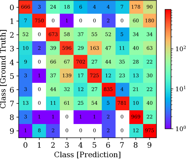
(a) Replay [43].

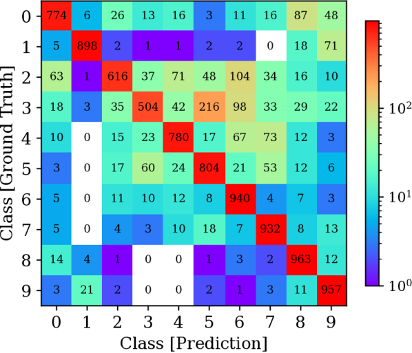
(b) MEMO [61].

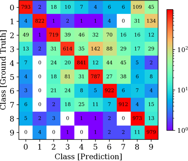
(c) $\text{BLCL}_{8[1,1,2,2]}$.

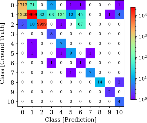
(d) Replay [43].

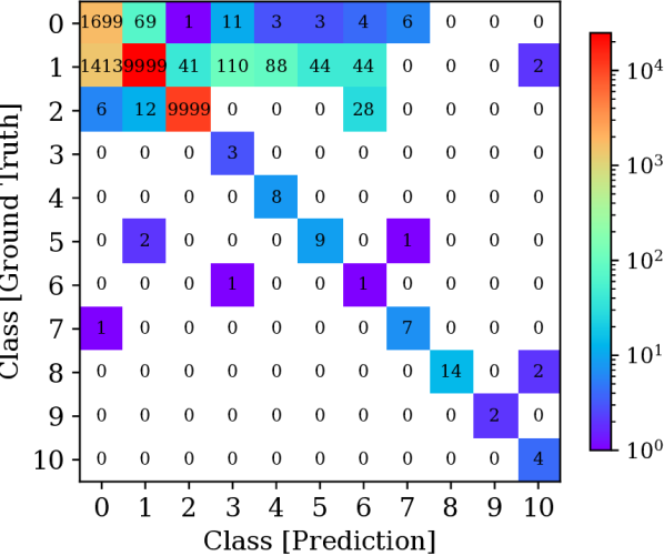
(e) MEMO [61].

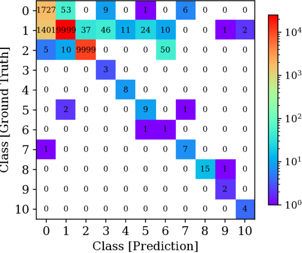
(f) $\text{BLCL}_{2[2,2,2,2,2]}$.

Figure 5: Confusion matrices of state-of-the-art methods and our Bayesian BLCL approach for the CIFAR-10 (a to c) and GNSS (d to f) datasets.

Confusion Matrices.

Figure 5 illustrates the confusion matrices subsequent to the final task to all test classes within the CIFAR-10 and GNSS datasets, employing the optimal baseline methodologies Replay [43], MEMO [61], and our proposed technique denoted as $\text{BLCL}_{8[1,1,2,2]}$ and $\text{BLCL}_{2[2,2,2,2,2]}$ with Bayesian weighting, respectively. On the CIFAR-10 dataset, MEMO demonstrates significant performance superiority over Replay for specific classes 0, 1, 4, 5, 6, and 7 (refer to Figure 5 compared to Figure 5). Notably, Replay exhibits pronounced confusion between classes 8 and 9 as well as the remaining classes, a misclassification mitigated by MEMO. Additionally, BLCL achieves a higher true positive rate than MEMO for classes 0, 2, 3, 4, and 9, thereby attaining an average accuracy of 86.57%, surpassing MEMO’s 84.78% (see Figure 5). Our approach effectively mitigates misclassifications, particularly between classes 3 and 6. On the GNSS dataset, a distinct resemblance exists between classes 1 and other classes (refer to Figure 4), resulting in misclassifications. While MEMO exhibits a higher false positive rate compared to Replay, their false negative rates remain equal, leading to Replay’s superior average accuracy of 95.45% versus MEMO’s 95.34% (compare Figure 5 with Figure 5). Leveraging enhanced representation learning via contrastive loss, our BLCL method effectively separates positive classes (3 to 10) into distinct clusters, thus reducing the false positive rate and yielding a higher F2-score of 0.713 while simultaneously decreasing the false negative rate (refer to Figure 5).

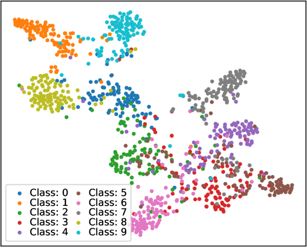
(a) Replay [43].

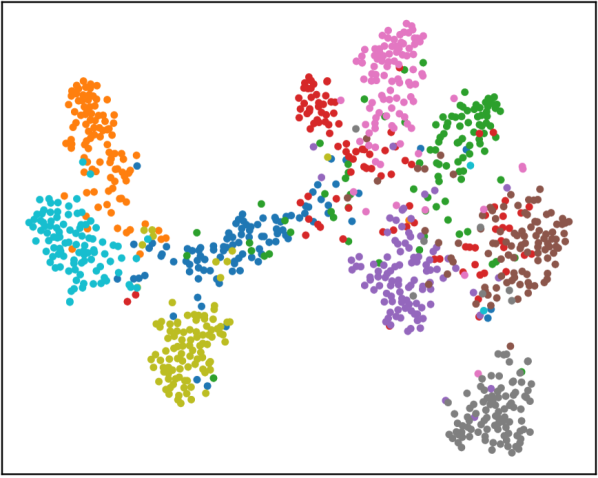
(b) MEMO [61].

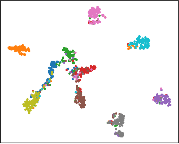
(c) $\text{BLCL}_{8[1,1,2,2]}$.

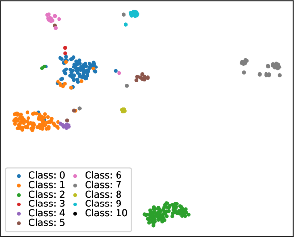
(d) Replay [43].

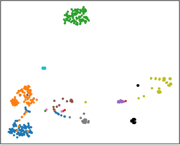
(e) MEMO [61].

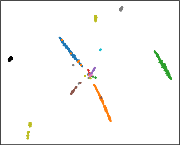
(f) $\text{BLCL}_{2[2,2,2,2,2]}$.

Figure 6: t-SNE [51] plots for the CIFAR-10 (a to c) and GNSS (d to f) datasets.

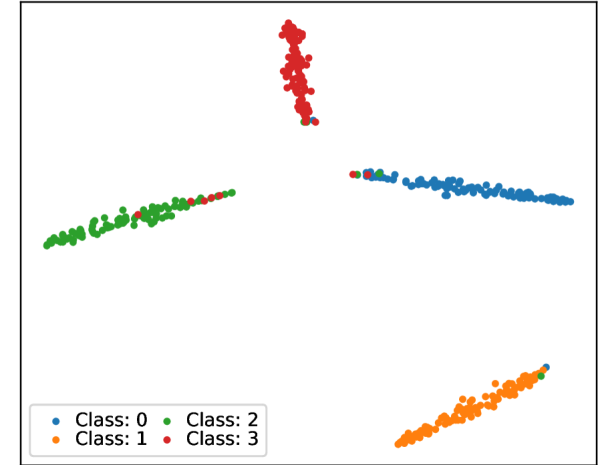
(a) Task 1.

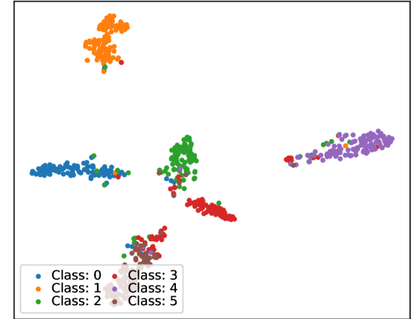
(b) Task 2.

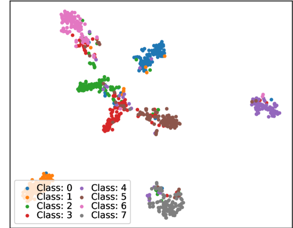
(c) Task 3.

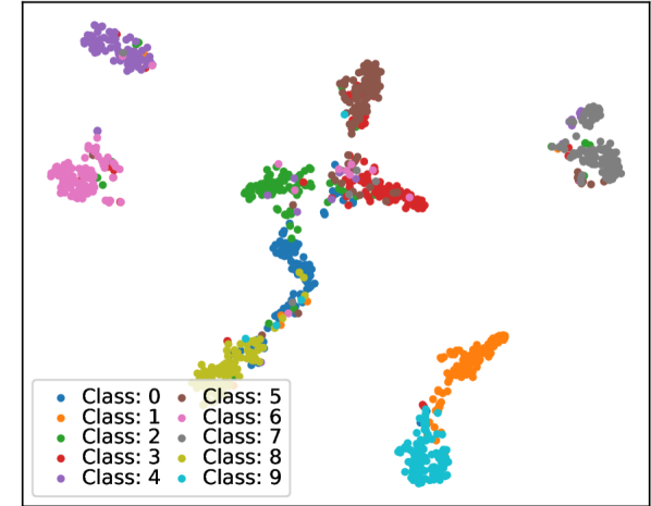
(d) Task 4.

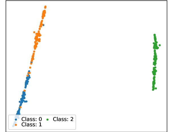
(e) Task 1.

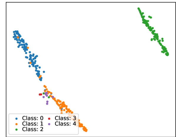
(f) Task 2.

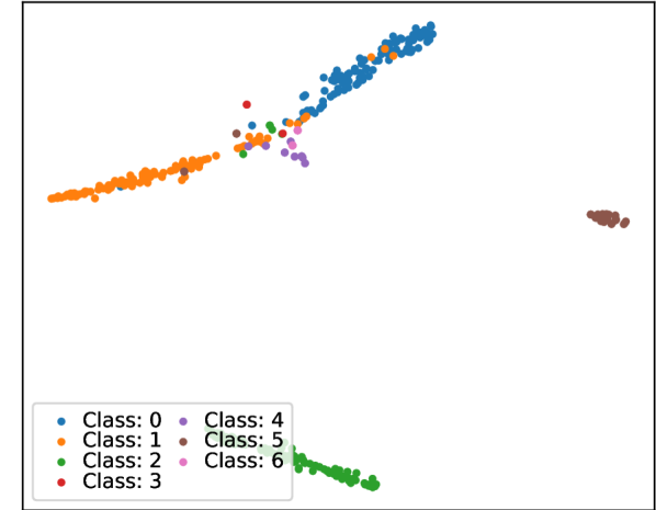
(g) Task 3.

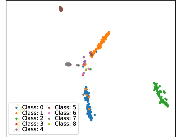
(h) Task 4.

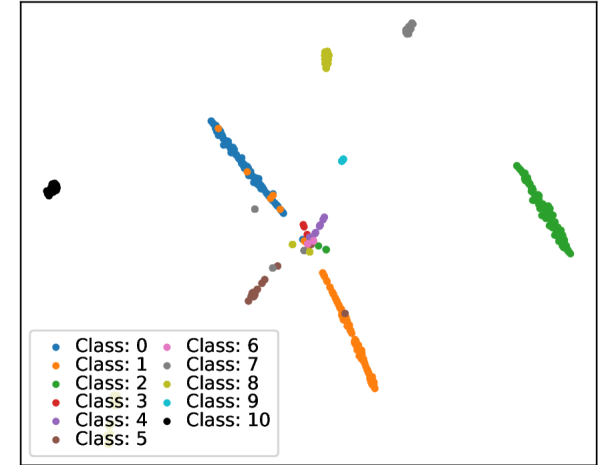
(i) Task 5.

Figure 7: t-SNE [51] plots for the CIFAR-10 (a to d) and GNSS (e to i) datasets after each task for our BLCL method.

Embedding Analysis.

The feature embedding of the last convolutional layer, with an output size of 512, is depicted in Figure 6. This embedding is generated using t-distributed stochastic neighbor embedding (t-SNE) [51] with a perplexity of 30, an initial momentum of 0.5, and a final momentum of 0.8. On the CIFAR-10 dataset, the Replay method (Figure 6) and MEMO method (Figure 6) demonstrate poor separation of clusters, resulting in the overlap of classes 2, 3, and 4, thereby leading to misclassification. This observation aligns with the findings presented earlier using confusion matrices (refer to Figure 5 and 5). Our proposed BLCL method (Figure 6), which incorporates contrastive loss, significantly reduces the intra-class distance and increases inter-class distance. However, some overlap persists, particularly for classes 0, 1, and 3, resulting in a higher rate of misclassification. Similar trends are observed in the GNSS dataset, where both Replay and MEMO methods exhibit overlapping samples with class 0, while the BLCL method only forms a small cluster with specific samples in the center of the embedding. Figure 7 visualizes the feature embeddings after each of the tasks. Specifically for the CIFAR-10 dataset (a to d), when adding clusters from new tasks, a large inter-class distance between clusters from previous classes are maintained. However, for the GNSS dataset (e to i), the samples from classes 3 and 4 from task 2 are added in-between the classes 0 to 2 due to a high similarity between the classes.

Table 3: Davies-Bouldin (DB) [11] ($\downarrow$) and Caliński-Harbasz (CH) [5] ($\uparrow$) scores.

	CIFAR-10		GNSS
Method	DB	CH	DB	CH
Finetune	7.29	2,716	1.48	7,958
EWC	2.12	1,365	1.34	4,799
LwF	2.14	848	1.97	4,565
iCarl	1.28	1,907	0.81	29,076
Replay	1.18	2,327	0.96	27,622
MEMO	1.78	1,736	1.15	14,066
BLCL	0.81	4,688	0.77	163,420

Cluster Analysis.

Subsequently, we compare the Davies-Bouldin (DB) [11] and Caliński-Harbasz (CH) [5] scores. DB is defined as the mean similarity measure between each cluster and its most similar cluster. This measure of similarity is the ratio of within-cluster distances to between-cluster distances. Consequently, clusters exhibiting greater separation and lesser dispersion will yield a superior score [18]. CH is a variance-ratio criterion, where a higher CH score relates to a model with better defined clusters, and is defined as the ratio of the sum of inter-clusters dispersion and of intra-cluster dispersion for all clusters. Table 3 summarizes the scores attributed to Finetune, EWC, LwF, iCarl, Replay, MEMO, and BLCL. Across both datasets, BLCL demonstrates a lower DB score and higher CH score in comparison to the baseline methods. This observation supports the assertion that BLCL results in a representation characterized by lower inter-class distances and enhanced clustering efficacy.

Parameter Counts.

Figure 8 provides a summary of the number of parameter counts pertaining to $\text{BLCL}_{6}$, $\text{BLCL}_{8}$, and $\text{BLCL}_{8[*]}$ configurations featuring dynamic specialized components across all tasks within the CIFAR-10 dataset. We observe that increasing the number of blocks within the specialized component from 6 to 8 results in a rise in parameter count from $2.1\cdot 10^{6}$ to $2.7\cdot 10^{6}$. However, this increase is accompanied by an improvement in accuracy, as illustrated in Table 1. By further decreasing the blocks in the specialized component from the full architecture $\text{BLCL}_{8[0,0,0,0]}$, the number of parameters can be further decreased, by still maintaining a high accuracy.

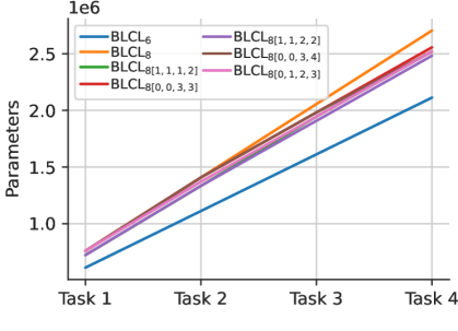
Figure 8: Number of parameters for each task.

6 Conclusion

In the context of the continual learning task, we proposed a method characterized by a dynamic specialized component. This component combines the CE loss with a prototypical contrastive loss by utilizing Bayesian learning principles. By employing dynamic loss weighting, our method effectively achieves a feature representation with reduced intra-class disparity and higher inter-class distance. Evaluations conducted on the CIFAR-10 and GNSS datasets demonstrate that our proposed technique outperforms the state-of-the-art MEMO, achieving an average accuracy of 84.78% and 95.34% respectively. Specifically, our method achieves accuracy rates of up to 86.57% on CIFAR-10 and 96.16% on the GNSS dataset with improved Davies-Bouldin and Caliński-Harabasz scores.

References

- [1] Jihwan Bang, Heesu Kim, YoungJoon Yoo, Jung-Woo Ha, and Jonghyun Choi. Rainbow Memory: Continual Learning with a Memory of Diverse Samples. In IEEE/CVF Intl. Conf. on Computer Vision and Pattern Recognition (CVPR), Nashville, TN, June 2021.
- [2] Jihwan Bang, Hyunseo Koh, Seulki Park, Hwanjun Song, Jung-Woo Ha, and Jonghyun Choi. Online Continual Learning on a Contaminated Data Stream with Blurry Task Boundaries. In IEEE/CVF Intl. Conf. on Computer Vision and Pattern Recognition (CVPR), New Orleans, LA, June 2022.
- [3] Magdalena Biesialska, Katarzyna Biesialska, and Marta R. Costa-jussà. Continual Lifelong Learning in Natural Language Processing: A Survey. In Proc. of the Intl. Conf. on Computational Linguistics, pages 6523–6541, Barcelona, Spain, Dec. 2020.
- [4] Tobias Brieger, Nisha L. Raichur, Dorsaf Jdidi, Felix Ott, Tobias Feigl, Johannes Rossouw van der Merwe, Alexander Rügamer, and Wolfgang Felber. Multimodal Learning for Reliable Interference Classification in GNSS Signals. In Proc. of the Intl. Technical Meeting of the Satellite Division of the Institute of Navigation (ION GNSS+), pages 3210–3234, Denver, CO, Sept. 2022.
- [5] Tadeusz Caliński and J. Harabasz. A Dendrite Method for Cluster Analysis. In Communications in Statistics, volume 3(1), pages 1–28, Sept. 1972.
- [6] Hyuntak Cha, Jaeho Lee, and Jinwoo Shin. : Contrastive Continual Learning. In Intl. Conf. on Computer Vision (ICCV), Montreal, QC, Oct. 2021.
- [7] Sungmin Cha and Taesup Moon. Sy-CON: Symmetric Contrastive Loss for Continual Self-Supervised Representation Learning. In arXiv preprint arXiv:2306.05101, June 2023.
- [8] Ting Chen, Simon Kornblith, Mohammad Norouzi, and Geoffrey Hinton. A Simple Framework for Contrastive Learning of Visual Representations. In Intl. Conf. on Machine Learning (ICML), volume 149, pages 1597–1607, July 2020.
- [9] Weihua Chen, Xiaotang Chen, Jianguo Zhang, and Kaiqi Huang. Beyond Triplet Loss: A Deep Quadruplet Network for Person Re-identification. In IEEE/CVF Intl. Conf. on Computer Vision and Pattern Recognition (CVPR), Honolulu, HI, July 2017.
- [10] Qing Da, Yang Yu, and Zhi-Hua Zhou. Learning with Augmented Class by Exploiting Unlabeled Data. In Proc. of the Intl. Conf. on Artificial Intelligence (AAAI), volume 28, 2014.
- [11] David L. Davies and Donald W. Bouldin. A Cluster Separation Measure. In IEEE Trans. on Pattern Analysis and Machine Intelligence (TPAMI), volume PAMI-1(2), pages 224–227, Apr. 1979.
- [12] Jia Deng, Wei Dong, Richard Socher, Li-Jia Li, Kai Li, and Li Fei-Fei. ImageNet: A Large-scale Hierarchical Image Database. In IEEE/CVF Intl. Conf. on Computer Vision and Pattern Recognition (CVPR), Miami, FL, June 2009.
- [13] Thanh-Toan Do, Toan Tran, Ian Reid, Vijay Kumar, Tuan Hoang, and Gustavo Carneiro. A Theoretically Sound Upper Bound on the Triplet Loss for Improving the Efficiency of Deep Distance Metric Learning. In IEEE/CVF Intl. Conf. on Computer Vision and Pattern Recognition (CVPR), Long Beach, CA, June 2019.
- [14] Jeff Donahua, Yangqing Jia, Oriol Vinyals, Judy Hoffmann, Ning Zhang, Eric Tzeng, and Trevor Darrell. DeCAF: A Deep Convolutional Activation Feature for Generic Visual Recognition. In Journal for Machine Learning Research (JMLR), volume 32(1), pages 647–655, 2014.
- [15] Arthur Douillard, Matthieu Cord, Charles Ollion, Thomas Robert, and Eduardo Valle. PODNet: Pooled Outputs Distillation for Small-Tasks Incremental Learning. In IEEE/CVF Europ. Conf. on Computer Vision (ECCV), volume 12365, pages 86–102, Nov. 2020.
- [16] Arthur Douillard, Alexandre Ramé, Guillaume Couairon, and Matthieu Cord. DyTox: Transformers for Continual Learning with DYnamic TOken eXpansion. In IEEE/CVF Intl. Conf. on Computer Vision and Pattern Recognition (CVPR), pages 9285–9295, 2022.
- [17] Ross Girshick, Jeff Donahue, Trevor Darrell, and Jitendra Malik. Rich Feature Hierarchies for Accurate Object Detection and Semantic Segmentation. In IEEE/CVF Intl. Conf. on Computer Vision and Pattern Recognition (CVPR), pages 580–587, 2014.
- [18] Maria Halkidi, Yannis Batistakis, and Michalis Vazirgiannis. On Clustering Validation Techniques. In Journal of Intelligent Information Systems, volume 17, pages 107–145, Dec. 2001.
- [19] Arman Hasanzadeh, Mohammadreza Armandpour, Ehsan Hajiramezanali, Mingyuan Zhou, Nick Duffield, and Krishna Narayanan. Bayesian Graph Contrastive Learning. In arXiv preprint arXiv:2112.07823, Aug. 2022.
- [20] Kaiming He, Xiangyu Zhang, Shaoqing Ren, and Jian Sun. Deep Residual Learning for Image Recognition. In IEEE/CVF Intl. Conf. on Computer Vision and Pattern Recognition (CVPR), Las Vegas, NV, June 2016.
- [21] Xin Huang, Yuxin Peng, and Mingkuan Yuan. MHTN: Modal-Adversarial Hybrid Transfer Network for Cross-Modal Retrieval. In Trans. on Cybernetics, volume 50(3), pages 1047–1059, 2020.
- [22] Zixuan Ke, Bing Liu, Hu Xu, and Lei Shu. CLASSIC: Continual and Contrastive Learning of Aspect Sentiment Classification Tasks. In Intl. Conf. on Empirical Methods in Natural Language Processing (EMNLP), pages 6871–6883, Nov. 2021.
- [23] Alex Kendall and Yarin Gal. What Uncertainties Do We Need in Bayesian Deep Learning for Computer Vision? In Advances in Neural Information Processing Systems (NIPS), Long Beach, CA, 2017.
- [24] Alex Kendall, Yarin Gal, and Roberto Cipolla. Multi-Task Learning Using Uncertainty to Weigh Losses for Scene Geometry and Semantics. In IEEE/CVF Intl. Conf. on Computer Vision and Pattern Recognition (CVPR), 2018.
- [25] James Kirkpatrick, Razvan Pascanu, Neil Rabinowitz, Joel Veness, Guillaume Desjardins, Andrei A. Rusu, Kieran Milan, John Quan, Tiago Ramalho, Agnieszka Grabska-Barwinska, Demis Hassabis, Claudia Clopath, Dharshan Kumaran, and Raia Hadsell. Overcoming Catastrophic Forgetting in Neural Networks. In Applied Mathematics, volume 114(13), pages 3521–3526, Mar. 2017.
- [26] Andreas Klaß, Sven M. Lorenz, Martin W. Lauer-Schmaltz, David Rügamer, Bernd Bischl, Christopher Mutschler, and Felix Ott. Uncertainty-aware Evaluation of Time-Series Classification for Online Handwriting Recognition with Domain Shift. In IJCAI-ECAI Intl. Workshop on Spatio-Temporal Reasoning and Learning (STRL), volume 3190, Vienna, Austria, July 2022.
- [27] Hyunseo Koh, Dahyun Kim, Jung-Woo Ha, and Jonghyun Choi. Online Continual Learning on Class Incremental Blurry Task Configuration with Anytime Inference. In Intl. Conf. on Learning Representations (ICLR), 2022.
- [28] Alex Krizhevsky. Learning Multiple Layers of Features from Tiny Images. 2009.
- [29] Ilja Kuzborskij, Francesco Orabona, and Barbara Caputo. From N to N+1: Multiclass Transfer Incremental Learning. In IEEE/CVF Intl. Conf. on Computer Vision and Pattern Recognition (CVPR), Portland, OR, June 2013.
- [30] Matthias De Lange, Rahaf Aljundi, Marc Masana, Sarah Parisot, Xu jia, Ales̆ Leonardis, Gregory Slabaugh, and Tinne Tuytelaars. A Continual Learning Survey: Defying Forgetting in Classification Tasks. In IEEE Trans. on Pattern Analysis and Machine Intelligence (TPAMI), volume 44(7), July 2022.
- [31] S. Lewandowsky and S.-C. Li. Catastrophic Interference in Neural Networks: Causes, Solutions, and Data. In F. N. Dempster & C. J. Brainerd (Eds.), Interference and Inhibition in Cognition, pages 329–361, 1995.
- [32] Zhizhong Li and Derek Hoiem. Learning Without Forgetting. In IEEE Trans. on Pattern Analysis and Machine Intelligence (TPAMI), volume 40(12), pages 2935–2947, Dec. 2018.
- [33] Lilang Lin, Jiahang Zhang, and Jiaying Liu. Bayesian Contrastive Learning with Manifold Regularization for Self-Supervised Skeleton Based Action Recognition. In IEEE Intl. Symposium on Circuits and Systems (ISCAS), Monterey, CA, May 2023.
- [34] Bin Liu, Bang Wang, and Tianrui Li. Bayesian Self-Supervised Contrastive Learning. In arXiv preprint arXiv:2301.11673, Jan. 2024.
- [35] Yaoyao Liu, Bernt Schiele, and Qianru Sun. RMM: Reinforced Memory Management for Class-Incremental Learning. In Advances in Neural Information Processing Systems (NIPS), 2021.
- [36] David Lopez-Paz and Marc’Aurelio Ranzato. Gradient Episodic Memory for Continual Learning. In Advances in Neural Information Processing Systems (NIPS), Long Beach, CA, 2017.
- [37] Zheda Mai, Ruiwen Li, Jihwan Jeong, David Quispe, Hyunwoo Kim, and Scott Sanner. Online Continual Learning in Image Classification: An Empirical Survey. In arXiv preprint arXiv:2101.10423, Oct. 2021.
- [38] Marc Masana, Xialei Liu, Bartlomiej Twardowski, Mikel Menta, Andrew D. Bagdanov, and Joost van de Weijer. Class-Incremental Learning: Survey and Performance Evaluation on Image Classification. In IEEE Trans. on Pattern Analysis and Machine Intelligence (TPAMI), volume 45(5), May 2023.
- [39] Felix Ott, Lucas Heublein, Nisha Lakshmana Raichur, Tobias Feigl, Jonathan Hansen, Alexander Rügamer, and Christopher Mutschler. Few-Shot Learning with Uncertainty-based Quadruplet Selection for Interference Classification in GNSS Data. In Intl. Conf. on Localization and GNSS (ICL GNSS), Feb. 2024.
- [40] Felix Ott, David Rügamer, Lucas Heublein, Bernd Bischl, and Christopher Mutschler. Auxiliary Cross-Modal Representation Learning with Triplet Loss Functions for Online Handwriting Recognition. In IEEE Access, volume 11, pages 94148–94172, Aug. 2023.
- [41] Nisha L. Raichur, Tobias Brieger, Dorsaf Jdidi, Tobias Feigl, Johannes Rossouw van der Merwe, Birendra Ghimire, Felix Ott, Alexander Rügamer, and Wolfgang Felber. Machine Learning-assisted GNSS Interference Monitoring Through Crowdsourcing. In Proc. of the Intl. Technical Meeting of the Satellite Division of the Institute of Navigation (ION GNSS+), pages 1151–1175, Denver, CO, Sept. 2022.
- [42] Nikhil Rasiwasia, Jose Costa Pereira, Emanuele Coviello, Gabriel Doyle, Gert R.G. Lanckriet, Roger Levy, and Nuno Vasconcelos. A New Approach to Cross-Modal Multimedia Retrieval. In Proc. of the ACM Intl. Conf. on Multimedia (ACMMM), pages 251–260, Oct. 2010.
- [43] R. Ratcliff. Connectionist Models of Recognition Memory: Constraints Imposed by Learning and Forgetting Functions. In Psychological Review, volume 97(2), pages 285–308, Apr. 1997.
- [44] Sylvestre-Alvise Rebuffi, Alexander Kolesnikov, Georg Sperl, and Christoph H. Lampert. iCaRL: Incremental Classifier and Representation Learning. In IEEE Intl. Conf. on Computer Vision and Pattern Recognition (CVPR), pages 2011–2010, Honolulu, HI, July 2017.
- [45] David Rolnick, Arun Ahuja, Jonathan Schwarz, Timothy Lillicrap, and Gregory Wayne. Experience Replay for Continual Learning. In Advances in Neural Information Processing Systems (NIPS), 2019.
- [46] Nikolaos Sarafianos, Xiang Xu, and Ioannis A. Kakadiaris. Adversarial Representation Learning for Text-to-Image Matching. In IEEE/CVF Intl. Conf. on Computer Vision (ICCV), pages 5814–5824, Seoul, Korea, 2019.
- [47] Florian Schroff, Dmitry Kalenichenko, and James Philbin. FaceNet: A Unified Embedding for Face Recognition and Clustering. In IEEE/CVF Intl. Conf. on Computer Vision and Pattern Recognition (CVPR), Boston, MA, June 2015.
- [48] Jake Snell, Kevin Swersky, and Richard Zemel. Prototypical Networks for Few-shot Learning. In Advances in Neural Information Processing Systems (NIPS), pages 4080–4090, Dec. 2017.
- [49] Mamatha Thota and Georgios Leontidis. Contrastive Domain Adaptation. In IEEE/CVF Intl. Conf. on Computer Vision and Pattern Recognition Workshops (CVPRW), Nashville, TN, June 2021.
- [50] Gido M. van de Ven, Hava T. Siegelmann, and Andreas S. Tolias. Brain-inspired Replay for Continual Learning with Artificial Neural Networks. In Nature Communications, volume 11(4069), Aug. 2020.
- [51] Laurens van der Maaten and Geoffrey Hinton. Visualizing Data Using t-SNE. In Journal for Machine Learning Research (JMLR), volume 9(86), pages 2579–2605, Nov. 2008.
- [52] Johannes Rossouw van der Merwe, David Contreras Franco, Jonathan Hansen, Tobias Brieger, Tobias Feigl, Felix Ott, Dorsaf Jdidi, Alexander Rügamer, and Wolfgang Felber. Low-Cost COTS GNSS Interference Monitoring, Detection, and Classification System. In MDPI Sensors, volume 23(7), 3452, Mar. 2023.
- [53] Fu-Yun Wang, Da-Wei Zhou, Han-Jia Ye, and De-Chuan Zhan. FOSTER: Feature Boosting and Compression for Class-Incremental Learning. In IEEE/CVF Europ. Conf. on Computer Vision (ECCV), volume 13685, pages 398–414, Oct. 2022.
- [54] Zifeng Wang, Zizhao Zhang, Chen-Yu Lee, Han Zhang, Ruoxi Sun, Xiaoqi Ren, Guolong Su, Vincent Perot, Jennifer Dy, and Tomas Pfister. Learning to Prompt for Continual Learning. In IEEE/CVF Intl. Conf. on Computer Vision and Pattern Recognition (CVPR), pages 139–149, 2022.
- [55] Yunchao Wei, Yao Zhao, Canyi Lu, Shikui Wei, Luoqi Liu, Zhenfeng Zhu, and Shuicheng Yan. Cross-Modal Retrieval with CNN Visual Features: A New Baseline. In Trans. on Cybernetics, volume 47(2), pages 449–460, Mar. 2016.
- [56] Yue Wu, Yinpeng Chen, Lijuan Wang, Yuancheng Ye, Zicheng Liu, Yandong Guo, and Yun Fu. Large Scale Incremental Learning. In IEEE/CVF Intl. Conf. on Computer Vision and Pattern Recognition (CVPR), pages 374–382, 2019.
- [57] Jiangwei Xie, Shipeng Yan, and Xuming He. General Incremental Learning with Domain-aware Categorical Representations. In IEEE/CVF Intl. Conf. on Computer Vision and Pattern Recognition (CVPR), pages 14351–14360, 2022.
- [58] Shipeng Yan, Jiangwei Xie, and Xuming He. DER: Dynamically Expandable Representation for Class Incremental Learning. In IEEE/CVF Intl. Conf. on Computer Vision and Pattern Recognition (CVPR), pages 3014–3023, 2021.
- [59] Bowen Zhao, Xi Xiao, Guojun Gan, Bin Zhang, and Shutao Xia. Maintaining Discrimination and Fairness in Class Incremental Learning. In IEEE/CVF Intl. Conf. on Computer Vision and Pattern Recognition (CVPR), pages 13205–13214, 2020.
- [60] Da-Wei Zhou, Qi-Wei Wang, Zhi-Hong Qi, Han-Jia Ye, De-Chuan Zhan, and Ziwei Liu. Deep Class-Incremental Learning: A Survey. In arXiv preprint arXiv:2302.03648, Feb. 2023.
- [61] Da-Wei Zhou, Qi-Wei Wang, Han-Jia Ye, and De-Chuan Zhan. A Model or 603 Exemplars: Towards Memory-Efficient Class-Incremental Learning. In arXiv preprint arXiv:2205.13218, Feb. 2023.