Recovery of Sparse Graph Signals
Abstract
This paper investigates the recovery of a node-domain sparse graph signal from the output of a graph filter. This problem, which is often referred to as the identification of the source of a diffused sparse graph signal, is seminal in the field of graph signal processing (GSP). Sparse graph signals can be used in the modeling of a variety of real-world applications in networks, such as social, biological, and power systems, and enable various GSP tasks, such as graph signal reconstruction, blind deconvolution, and sampling. In this paper, we assume double sparsity of both the graph signal and the graph topology, as well as a low-order graph filter. We propose three algorithms to reconstruct the support set of the input sparse graph signal from the graph filter output samples, leveraging these assumptions and the generalized information criterion (GIC). First, we describe the graph multiple GIC (GM-GIC) method, which is based on partitioning the dictionary elements (graph filter matrix columns) that capture information on the signal into smaller subsets. Then, the local GICs are computed for each subset and aggregated to make a global decision. Second, inspired by the well-known branch and bound (BNB) approach, we develop the graph-based branch and bound GIC (graph-BNB-GIC), and incorporate a new tractable heuristic bound tailored to the graph and graph filter characteristics. Finally, we propose the graph-based first order correction (GFOC) method, which improves existing sparse recovery methods by iteratively examining potential improvements to the GIC cost function through replacing elements from the estimated support set with elements from their one-hop neighborhood. We conduct simulations over the square grid graph and the Erdős-Rényi graph that demonstrate that the proposed sparse recovery methods outperform the orthogonal matching pursuit (OMP) method, the Lasso method, and the BNB method with regularization in terms of support set recovery accuracy, and without a significant computational overhead.
Index Terms:
Graph signal processing (GSP), support set recovery, double sparsity, generalized information criterion (GIC), graph signals, graph filtersI Introduction
gsp theory extends classical time-varying signals to irregular domains represented by graphs [2, 3, 4]. The graph under consideration may represent a physical network, such as electrical or sensor networks, or a virtual network, such as social networks, or it may encode statistical dependencies among the signal values. Recent developments in graph signal processing (GSP) encompass a wide array of processing tools, including graph spectral analysis [5, 6], anomaly detection [7], sampling and signal recovery [8, 9, 10, 11, 12, 13, 14], verification of graph smoothness [15, 16], and graph filter design [2, 3, 17, 18]. However, limited attention has been paid to developing GSP-based techniques for the sparse recovery of node-domain sparse graph signals.
Signal modeling based on sparse representations is used in numerous signal and image processing applications [19, 20, 21, 22]. Sparse recovery methods can be categorized into the following main groups: convex relaxations techniques, often using methods such as -norm minimization or basis pursuit [19, 23, 24, 25, 26], non-convex optimization techniques [27, 28, 29], and greedy algorithms [30, 20, 31, 32, 33]. Bayesian inference approaches estimate the sparse signal by incorporating prior information, whereas other methods use knowledge of dictionary matrix structure. In network science, compressed sensing and group testing have been discussed in [34, 35, 36], while diffusion processess have been discussed in [37, 38, 39, 40, 41]. Additionally, several GSP works have investigated the reconstruction of bandlimited graph signals where the measurement vector belongs to a subspace defined by a small number of graph frequencies [42, 43, 44].
Recently there has been growing interest in setups where a node-domain sparse graph signal is filtered by a graph filter . In this case, the output signal is referred to as a diffused sparse graph signal [45]. Modeling diffusion processes over graphs by graph filters is valuable due to the ability to capture local interactions among nodes [46, 47, 48, 49]. Diffused sparse graph signals can be used for modeling many real-world network scenarios. For instance, in social networks, these signals can be used for opinion forming [50] and finding the origin of a rumor [51]. In biological networks, they enable the analysis of the spread of a disease [52], and in computer networks, they can be used to locate malware [53]. In power systems, they may be used for locating anomalies in power signals [54, 55]. In the field of GSP, diffused sparse graph signals have been studied in several problems, such as bandlimited graph signal reconstruction [56]. Blind deconvolution, in which both the graph filter and the sparse input are estimated, has been discussed in [45, 46, 57, 58]. System identification, considered in [47, 45], refers to the case where the sparse signal is known, but the graph filter coefficients are estimated. The sampling of diffused sparse graph signals is discussed in [59]. However, in the applications discussed above, the sparse recovery does not exploit the GSP-based modeling of the sparse graph signals. Instead, the sparse recovery is typically done by sparse approximations, usually relaxation, or with a tailored solution that uses the specific properties of the application.
This paper establishes sparse recovery methods for graph signals using the generalized information criterion (GIC) as the cost function, and practical assumptions including the sparsity of the underlying graph. A direct solution for the GIC-based problem necessitates an exhaustive search, whose complexity grows exponentially with the size of the graph, rendering it impractical. We propose three graph-based sparse recovery methods that harvest the double sparsity imposed by the graph and the graph signal. The first method, the graph-based multiple generalized information criterion (GM-GIC) method, identifies and partitions a set of suspected nodes and then applies a local GIC on each partition, which significantly reduces the computational overhead of the GIC-based approach. The second method, the graph-based branch and bound GIC (Graph-BNB-GIC) method, further mitigates the computational demands by iteratively searching over the candidate support sets of the sparse graph signals (the same sets as in the GM-GIC method). This method is developed based on the branch and bound (BNB) method [60, 61] with a heuristic graph-based upper bound that exploits the double sparsity and the graph properties. The third method, the graph-based first order correction (GFOC) method, builds upon existing sparse recovery techniques and improves them in terms of the GIC cost function by replacing elements from the estimated support set with elements from their one-hop neighborhood. Our simulations over the square grid graph and an Erdős-Rényi graph demonstrate that the proposed methods outperform the state-of-the-art orthogonal matching pursuit (OMP), Lasso, and BNB with regularization methods in terms of the support set recovery accuracy, and without a significant computation overhead.
The paper is organized as follows. Section II presents the necessary background and outlines the problem formulation. In Section III, we analyze the dictionary matrix for the proposed graphical setting. We describe both the GM-GIC and Graph-BNB-GIC methods in Section IV, followed by the presentation of the GFOC method in Section V. In Section VI, we present the simulation results, and the conclusions are provided in Section VII.
Notations: In the rest of this paper, vectors and matrices are denoted by boldface lowercase and uppercase letters, respectively. The th element of the matrix is denoted by . The vector is a subvector of with the elements indexed by the set , and is the submatrix of consisting of the columns indexed by . In particular, denotes the th column of . The projection matrix into the subspace is given by
| (1) |
The operators , , , and denote the Euclidean norm, norm, zero semi-norm, and set cardinality. The identity matrix is denoted by .
II Problem Formulation
In this section, we formulate the problem of recovering a sparse graph signal from the outputs of a graph filter. First, in Subsection II-A, we present relevant GSP background. Then, in Subsection II-B, we outline the graphical setting considered. Finally, in Subsection II-C, we present the recovery problem addressed in this paper.
II-A Background: Graphs and Graph Filters
Consider an undirected weighted graph , which consists of a set of nodes (vertices) , a set of edges , and a set of weights . A graph signal is a mapping from the graph nodes into a real vector:
| (2) |
A graph shift operator (GSO), , is a linear operator applied on graph signals that satisfies
| (3) |
where the geodesic distance between nodes and , , is the number of edges on the shortest path between these nodes. According to (3), the non-zero elements of are the diagonal elements (i.e. ) or the elements that are associated with an edge (i.e. ). As a result, by applying a graph shift operator on a graph signal , each element of the shifted signal, , is a linear combination of the signal elements in its one-hop neighborhood:
| (4) |
where
| (5) |
Thus, the transformation by the graph shift operator can be computed locally at each node by aggregating the values of the input signal within the one-hop neighborhood of each node.
A shift-invariant graph filter, , is defined as a polynomial of the graph shift operator [3, 4]:
| (6) |
where are the coefficients of the graph filter and is the graph filter order. By substituting (3) in (6) it can be verified that the th element of satisfies
| (7) |
Consequently, each element of the filtered signal, , is a linear combination of the signal elements in its -hop neighborhood. Hence, the filtered signal satisfies
| (8) |
where is defined in (5). Thus, the filtered signal can be computed locally at each node by aggregating the values of the input signal within the -hop neighborhood of each of the nodes. We conclude with the following lemma.
Lemma 1.
Let, and be two nodes with a geodesic distance larger than , i.e. . Then, their associated graph filter columns and are orthogonal, i.e.
| (9) |
II-B Assumptions on the Graphical Setting
In this paper, we consider the following assumptions on the underlying graph and the graph filter.
-
A.1
The maximum nodal degree (the maximal number of edges connected to one node) of the graph is considered small, i.e. .
-
A.2
The graph filter is a polynomial of the graph shift operator as defined in (6). Aditionally, the graph filter degree, , is small with respect to (w.r.t.) the number of nodes, i.e. .
The meaning of these assumptions is as follows. Assumption A.1 enforces a sparse connectivity pattern on the underlying graph, i.e. sparse graph, where the number of edges is limited by , which is far fewer than the maximum possible number of edges (). Furthermore, this sparse connectivity pattern is enforced uniformly in the sense that any subgraph of the graph is also sparse, where the restriction in Assumption A.1 also applies to the subgraph. Assumption A.2 restricts the number of elements in each -hop neighborhood by imposing a small value for . The structure of the polynomial graph filter shown in (6) also implies that, in general, the values of the filtered signal, , in (8), are more significant for indices associated with nodes closer to the nodes in . Here, refers to the support set of the sparse signal. Therefore, combining Assumptions A.1-A.2 has a direct impact on the filtered signal outputs in (8), which are shown to be linear combinations of signal elements in their -hop neighborhoods. Consequently, only a portion of the filtered signal outputs hold substantial information on the input signal.
The graph filter in (6) under Assumptions A.1-A.2 can be used to model a variety of GSP tasks, including signal reconstruction, blind deconvolution, sampling and system identification [45, 46, 57, 47, 59]. Additionally, this framework can be used for modeling real-life applications in social networks [50, 51], in biological networks [52], in computer networks [53], in wireless sensor networks [5], and in power systems [54, 55]. It is worth noting that in the context of power systems, the average nodal degree is generally very low (usually between 2 to 5) and does not increase with the network size [62]. This property is also common in other infrastructure systems, such as water and transportation systems.
II-C Recovery of Sparse Graph Signals
In this paper, we aim to recover the source of a diffused sparse graph signal [45] from noisy observations under Assumptions A.1-A.2. That is, we are interested in recovering the graph signal , defined in (2), from the observation vector , where the following measurement model is assumed:
| (11) |
In this model, is the graph filter, defined in (6), which is a sparse dictionary matrix that satisfies Assumptions A.1-A.2. The noise is modeled by a zero-mean Gaussian vector, , with a known covariance matrix, , i.e. . Additionally, the unknown graph signal is assumed to be sparse:
| (12) |
where is the semi-norm and the sparsity parameter indicates the sparsity level. Hence, there exists a set of nodes, , referred to as the signal support set such that
| (13) |
That is, only the elements in the support set may correspond to non-zero elements of .
Based on (11)-(13), the sparse recovery problem can be formulated as (Eq. (1) in [20])
| (14) |
The inner minimization problem in (14) is a least squares (LS) problem with the solution (see, e.g. p. 225 in [63]):
| (15) |
By substituting (15) in (14) we obtain the following support set recovery problem:
| (16) |
where is the projection matrix onto the suspace , defined in (1). The last equality in (16) is obtained by using the projection matrix property (see Theorem 2.22 in [64]):
removing the constant , and rearranging the problem.
The support set recovery problem presented in (16) qualifies for any sparse signal and dictionary matrix , not necessarily over graphs, and is valid as long as is a nonsingular matrix. This problem can be viewed as a multiple-hypothesis testing problem, where under each hypothesis, the sparse signal has a different support set [65], which belongs to the following set of candidate sets:
| (17) |
A direct solution of the support set recovery in (16) tends to overfit by selecting support sets with larger cardinality than the true support set. To mitigate this problem, we use the well-known GIC model selection method, which is a generalization of various criteria, such as the Akaike information criterion (AIC) and the minimum description length (MDL). For the considered problem, the GIC is given by [66]
| (18) |
Compared to (16), the GIC in (18) includes an additional penalty function component, , which depends on the support set cardinality and mitigates the risk of overfitting. After solving (18), the sparse signal recovery solution can be obtained by substituting in (15).
In practice, an exact solution for (18) requires an exhaustive search over all optional support sets, which is infeasible. To overcome the unfeasibility of the combinatorial search, we propose using the graphical properties imposed by Assumptions A.1-A.2, and the double sparsity of the graph and the graph signal. The analysis for this setting is presented in Section III, and the proposed low-complexity support set recovery methods are developed in Section IV and Section V.
III Dictionary Matrix Analysis
In this section, we analyze the dictionary matrix atoms (i.e. graph filter columns) based on the underlying graphical structure and Assumptions A.1-A.2. This analysis forms the basis for the proposed sparse recovery methods in Sections IV and V.
Taking into account that for any , (see (13)), the filtered signal satisfies
| (19) |
where is the th column of . Hence, the filtered signal, , can be viewed as a linear combination of dictionary atoms (graph filter columns). In addition, if two dictionary atoms correspond to nodes and with a geodesic distance larger than , i.e. , then the projection matrix definition and (9) imply that
| (20) |
where is the projection matrix onto the single-column space (see the definition in (1)).
Now, let be the -order neighborhood of the set . Hence,
| (21) |
where is defined in (5). Thus, assume that , then, left-multiplying (19) by and substituting (20) results in
| (22) |
Therefore, left-multiplying the measurement model in (11) by and substituting (22) results in
| (23) |
for all . Consequently, the dictionary atoms, indexed by nodes outside the set in (III), contain only noise. That is, the dictionary matrix elements that contain information on the sparse graph signal are only those included in the neighborhood of , .
The following theorem establishes a bound on the cardinality of the set from (III) as a function of the graph filter degree , the graph structure, and the sparsity level . This theorem is important as it provides constraints on the size of a reduced set of dictionary atoms containing signal information. It offers two key advantages: first, it reduces the number of candidate support sets used to construct the feasible set in (18); second, observing a reduced set of dictionary atoms enhances processing flexibility, where a smaller set may be viewed as multiple (unrelated) regions across the graph, while the entire node set, , must be regarded as a single region.
Theorem 2.
The cardinality of the set is bounded by
| (24) |
where is the maximum degree of the graph.
Proof.
Since is the maximal degree of the graph, we obtain that each node in the graph has up to neighboring nodes, and each of those neighboring nodes can, in turn, have up to neighbors, and so on. As a result, the size of the neighborhood of a single node satisfies
| (25) |
By summing all the th bounds in the form of (25) for , we obtain
| (26) |
Therefore, since under the sparsity assumption in (12), we conclude that the -neighborhood of is bounded by the right hand side (r.h.s.) of (24). ∎
The bound in (24) depends on the sparsity level, , the maximal degree of the graph, , and the graph filter degree, , that are all considered to be small based on (12), Assumption A.1, and Assumption A.2, respectively. In contrast, the bound is independent of the size of the graph, i.e. the number of nodes, . Thus, for large networks it can be assumed that the bound is significantly lower than the actual number of nodes:
| (27) |
Consequently, by substituting (27) in (24) we obtain
| (28) |
The significance of the result in (28) lies in the observation that the number of dictionary atoms containing information about the sparse signal is much smaller than the total number of dictionary atoms that are required for searching for the optimal GIC in (18). As a result, any sparse recovery method that employs a search algorithm (and not just the GIC in (18)) can significantly reduce its computational complexity by focusing on the reduced set of dictionary atoms associated with the nodes in instead of on the entire set associated with all nodes in .
Moreover, it should be noted that the bound in (24) is not tight. This is because we may have overlaps between the -order neighborhoods of the nodes in and overlaps within the -order neighborhoods of individual nodes (see first and second inequalities in (26), respectively). As a result, in practice, the number of elements in can be considerably lower than its bound in (24). This further emphasizes the advantage of reducing computational complexity by searching over instead of .
Due to the graph filter structure defined by (6)-(8), and the sparse connectivity of the graph imposed by Assumption A.1, we can expect a decrease in the energy of the projection of over the elements in as the distance from the elements in increases. Thus, there exists a set such that
| (29) |
where is small. Therefore, it is implied that the dictionary matrix elements that contain information on the filtered signal is included in the set , which is a subset of the -hop neighborhood of , , . As a result, when the sparse signal input is distributed across different regions of the graph, the nodes within , which are composed of only a small portion of the graph nodes, will also tend to be in distant regions of the graph.
IV Sparse Recovery of Graph Signals
In this section, we propose two methods for solving the GIC support set recovery problem in (18) under the GSP measurement model in (11). The analysis in Section III provides the basis for these methods, since it enables searching for the optimal support set over a reduced set of dictionary atoms. In Subsection IV-A, we present the GM-GIC method, which involves a node partitioning followed by the implementation of the GIC locally on each partitioned subset. In Subsection IV-B, we present the Graph-BNB-GIC method, which is based on the BNB method [60, 61], and involves an upper bound that is derived based on the underlying graphical structure, thus significantly enhancing the traceability of this method.
IV-A GM-GIC
In this subsection, we outline the rationale and then present the methodology of the GM-GIC method.
IV-A1 Rationale
The analysis in Section III implies that the true support set of the signal, , is included in the set from (29). Considering that , in many cases the elements in are located in different regions across the graph as discussed below (29). Thus, in many cases the set can be divided into subsets, , such that
| (30) |
for any two subsets and from , where and . The partial support set in the th area, denoted as , is defined as . It should be noted that is a partition of the true support set , since there is no overlap between these subsets and .
Based on (9) in Lemma 1, the partition in (30) implies that any two dictionary atoms associated with two elements from two different subsets are orthogonal, i.e.
| (31) |
for any and where . Hence, by definition, the column spaces associated with two different subsets are orthogonal, i.e. . Therefore, the projection of , where , onto satisfies
| (32) |
for any and where . This implies that the partial support set does not affect the measurements in other subsets , . Thus, instead of searching for the true support set, , over the entire set , we aim to find the partial support sets, , by searching across the smaller subsets . In Algorithm 1 presents an algorithm to partition to connected sets that satisfy (30).
| (33) |
Proof.
Let be the subsets obtained from Algorithm 1, and let and be selected from different subsets. For the sake of contradiction, assume that . Since and satisfy , they must be connected by one of the edges in the set , i.e. , where is defined in (33). However, this contradicts our assumption since only if and are in the same connected component . Therefore, we can conclude that when and are in different subsets from , then the geodesic distance between them satisfies . Correspondingly, the subsets obtained from Algorithm 1 satisfy (30). ∎
IV-A2 Methodology
The GM-GIC method consists of four steps. In the first step, based on (23), we estimate the set described in (29) by applying the generalized likelihood ratio test (GLRT) for each on the following binary hypothesis testing problem:
| (34) |
This hypothesis testing can be understood as the task of detecting a signal embedded in Gaussian noise. In this case, the signal is projected onto a smaller subspace, , under both hypotheses. Under , the signal is presumed to be present in the subspace, whereas in the subspace encompasses solely the noise.
The GLRT for the hypothesis testing in (34) is defined for each as (see, e.g. p. 201 in [67])
| (35) |
where is a user-defined threshold parameter. Thus, the set is estimated according to the binary detector in (35), which is defined for each , by
| (36) |
In the second step, we use the node partition algorithm in Algorithm 1 with the input from (36) to obtain the subsets . In the third step, we solve the support set recovery problem in (18) for each subset separately. That is, we estimate the partial support set by
| (37) |
It is noted that for any , the partial support set, , may be smaller than or equal to the subset from which it is recovered, . The total support set of the sparse vector is then computed as the union of the partial estimates obtained from (37), as follows:
| (38) |
It should be noted that in (37) we impose the condition that the size of the support set should not exceed the sparsity parameter, , for each subset separately. As a result, we can ensure that the cardinality of is always less than or equal to for any . However, the same restriction does not apply to the union set in (38), which means that the cardinality of may be greater than , and thus, it may not be in the feasible set of the original optimization problem in (18). In order to address this issue, in the fourth step, sparsity-level correction is performed by solving the recovery in (16) for . That is, we compute the final estimator of the support set by
| (39) |
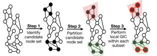
The GM-GIC method is summarized in Algorithm 2 and illustrated in Fig. 1.
IV-B Graph-BNB-GIC
In this subsection we present a new Graph-BNB-GIC method for solving the GIC problem in (18). To this end, we reformulate the GIC problem in (18) as an integer programming optimization problem, and then derive the Graph-BNB-GIC method. The Graph-BNB-GIC, is a BNB-based method (see, e.g. [60, 61]) with novel graph-based designs for the branching and bounding steps.
IV-B1 New formulation
By using the Boolean vector , we adress the GIC problem in (18) as the following integer programming optimization problem:
| (40) |
where is the support set of , i.e. the set of indices corresponding to non-zero elements of that are in this case equal to 1. It can be verified that the problem in (IV-B1) is equivalent to the problem in (18) (provides the same solution). In the new formulation, each node can be fixed to either or . In this way we can impose additional information on the specific node, and determine whether it is part of the support set or not. The added flexibility is essential for the branch step, which is described next.
IV-B2 Branch
Without loss of generality, we assume that the graph node indices are ordered according to their single-node projected energy, i.e.
| (41) |
According to the discussion around (29), nodes included in the true support set of the signal , , are associated with smaller indices in (41). Moreover, dictionary atoms associated with nodes indexed larger than , w.r.t. to the ordering in (41), are not expected to contain substantial information on the filtered signal, . Based on the ordering in (41), we describe the branch step as follows. By selecting index , we form the following two problems: the first problem is
| (42) |
and the second problem is
| (43) | |||
| (44) |
In other words, we fix the value of to in the first subproblem, which means that the first node is not part of . In the second subproblem, we set the value of to be , which means that the first node is part of . The problems in (IV-B2) and (43) are subproblems of the original problem in (IV-B1) since they have the same cost function and constraints as the original problem with one additional variable fixed. Each of these subproblems is an integer programming optimization problem, with Boolean variables. The optimal value of the original problem is the maximum between the optimal values of the two subproblems.
The division of (IV-B1) to the two subproblems in (IV-B2)-(43) is the first branch step performed in our algorithm. The second branch step is obtained by splitting one of the above subproblems, once with and once with , following the order in (41). By continuing in this manner, we form a partial binary tree of subproblems (see our illustration in Fig. 2). The root is the original problem depicted in (IV-B1). This problem is split into the two child subproblems in (IV-B2) and (43). The second iteration yields another two children of one of the original children. In general, the subproblems can be written as
| (45) |
where is the set of Boolean variables fixed to and is the set of Boolean variables fixed to . It can be seen that in the optimization problem in (IV-B2), the equality constraints determine from the elements of . Hence, each subproblem could be represented by the notation , e.g. , , and represent (IV-B1), (IV-B2), and (43), respectively. Additionally, splitting (IV-B2) into two subproblems is achieved by adding node once to the set and once to the set . Hence, the index used to split a leaf node is determined based on the ordering in (41), where a leaf node refers to a node in the partial binary tree that does not have children nodes. Figure 2 illustrates two iterations of the branch step.
IV-B3 Bound
When applied to large models, standard BNB search algorithms (see e.g. [60]) that use theoretical upper and lower bounds may take substantial amounts of computing time for mixed Boolean convex problems. Using a heuristic bound to replace the upper or lower bound might achieve a significant speedup in the BNB search procedure. For example, [68, 69] showed, for the optimal network design problem, that using a heuristic bound may dramatically reduce the computational complexity with a minor effect on the performance. Therefore, based on the analysis in Subsection III, we propose a heuristic upper bound alongside a theoretical lower bound for (IV-B2).
Based on the analysis in Subsection III, which stems from Assumptions A.1-A.2, we propose the following heuristic upper bound on the optimal objective of (IV-B2):
| (46) |
where . The heuristic bound states that the maximum cost function in (IV-B2) is bounded by the superposition of:
-
1.
The cost function associated with the elements in that are already fixed as (the elements in ): ;
-
2.
The cost function associated with the highest individual contributor within the elements not yet determined, i.e. node where , multiplied by the number of elements that can be added to without exceeding the sparsity limit: .
The lower bound on the optimal solution of (IV-B2) is obtained by taking the cost function of one of the elements in the feasible set. Specifically, we consider the element in which the undetermined elements (i.e., the elements in ) are set to zero. All the elements in are determined for this case, and the non-zero elements correspond to the set . Thus, the lower bound for (IV-B2) is set to
| (47) |
Hence, the lower bound for (IV-B2) is equivalent to the cost function of the support set . It is noted that the lower bound used is a valid bound that is always lower than the optimal value of the solution of (IV-B2). This can be verified by observing the fact that is in the feasible set of the maximization problem in (IV-B2), and thus its cost would always be lower than or equal to the optimal cost function.
IV-B4 Remarks
We conclude the discussion on the bounds with the following two remarks that demonstrate the relationships between the lower and upper bounds in special cases.
Remark 1.
By substituting (47) in (IV-B3) we obtain
| (48) |
Thus, if , then the lower bound and upper bound are equal, i.e., . The rationale behind this result is that in this case, the subproblem already reaches the maximal support set cardinality, , and, thus, the associated leaf node in the binary tree should not be further divided.
Remark 2.
Due to the ordering in (41), it can be verified that if , then . Hence, from (29) we obtain that . Thus, by considering a low degree of noise, it can be assumed that
| (49) |
By substituting the result from (49) in (1), we obtain that the difference between the upper and lower bound in (1) when satisfies
where the sparsity parameter indicates the the sparsity level of the signal, , and is defined in (29). This result implies that observing support set elements with nodes outside cannot improve the support set recovery results. Consequently, the result shows that in the worst-case scenario of the algorithm, it terminates after observing all support set combinations within the set from (29). Hence, in its worst case, the algorithm requires an order of flops (see Subsection IV-C for a comparison with the GIC and GM-GIC methods).
IV-B5 Algorithm
The algorithm for implementing the Graph-BNB-GIC method is initialized by the set containing only the root node, which is characterized by the sets . At each iteration, branching occurs from the leaf node with the smallest depth, where if there are multiple leaves with the smallest depth, then the leaf with the largest upper bound is selected. That is, the leaf node is selected by
| (50) |
The branching is performed by the branch step outlined in Subsection IV-B2. Hence, to generate , all elements in are duplicated excluding the selected leaf node. The sets of the selected node, , are then split into two child nodes: and , where . The algorithm terminates when , where and denote the maximum upper bound and maximum lower bound across all leaf nodes (nodes in ), respectively. In this case, the maximum upper bound and maximum lower bound belong to the same leaf, and the set , which is associated with this leaf, represents the estimated support set (i.e. the algorithm output). Additionally, if the upper bound of a leaf is smaller than the global lower bound, , then it is pruned (removed from the set ) since the cost function associated with any of its potential descendants is assumed lower than its upper bound and that the global lower bound represents a cost function of a feasible solution. The proposed Graph-BNB-GIC method is summarized in Algorithm 3.
IV-C Computational Complexity
The main goal of this work is to develop graph-based low-complexity methods for support set recovery of sparse graph signals. Specifically, we aim to design low-complexity methods that approximate the solution of the GIC optimization in (18), since a direct solution requires an exhaustive search with computational complexity that grows exponentially with the size of the graph. In particular, the exhaustive search requires floating-point operations (flops), as can be seen in (18). The computational complexity of the GM-GIC method from Algorithm 2 is primarily determined by the computations of the local GIC on the largest subset, and thus requires flops. Hence, its complexity is significantly lower than those of the GIC methods, where and from (29) and Theorem 2, . The Graph-BNB-GIC method from Algorithm 3 is anticipated to have an even lower computational burden compared with the GM-GIC method, due to its iterative nature. However, as shown in Remark 2, in its worst-case scenario it requires an order of flops. Consequently, even in the worst case, the computational complexity of the Graph-BNB-GIC method is significantly lower than that of the GIC method.
V GFOC
In this section, we present the GFOC method, which is a new method for correcting existing estimated support sets of the sparse graph signal, . This correction is obtained by optionally replacing the support set elements with nodes from their one-hop neighborhood, . The initial estimated support set, , can be obtained by any sparse recovery method, including standard techniques (such as the OMP [31] and Lasso [23] methods), as well as the GM-GIC and Graph-BNB-GIC methods proposed in Subsection II-C.
V-A Method
The proposed GFOC method receives as an input a support set estimate, , provided by any sparse recovery algorithm, along with the system measurements and the information regarding the underlying graph. Then, the GFOC method goes over the estimated support set elements. For each element (i.e. each node ), it examines whether the GIC increases when the element is replaced with one of the nodes in the one-hop open neighborhood set
| (51) |
where is defined in (5) (with ). If the GIC increases, then the method propagates by replacing the th support set element with its neighbor, i.e. the element in (51) that maximizes the GIC. Otherwise, the th element stays in the estimated support. It is noted that if the GFOC method input is infeasible, i.e. , then the input can be corrected by selecting the indices associated with the largest values in where . The GFOC method is summarized in Algorithm 4. In addition, the following simple example illustrates the process of the GFOC method for a -node graph.
Example 1.
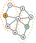
Fig. 3 illustrates the following scenario: the GFOC method receives as input a set of measurements , a graph filter , and an estimated support set . The GFOC method starts by examining the first-order neighborhood of node (the orange area). Specifically, it finds such that is the optimal support set that maximizes the GIC cost function in (18) within the sets: and . Similarly, it examines the first-order neighborhood of node (the green area). Hence, it finds such that is the optimal support set that maximizes the GIC cost function in (18) within the sets , and .
V-B Discussion
The GFOC method is derived based on the GIC in (18) and the analysis in Section III, derived following Assumptions A.1-A.2. Specifically, based on the discussion around (29), it can be inferred that when estimating the support set, if some errors occur, they are likely to be caused by the accidental inclusion of nodes in close proximity to the elements in the true signal support set . These mistakenly included nodes may be in addition to, or instead of, some of the elements in . In response to this possible error, Algorithm 4 proposes examining the immediate neighborhood of elements within the estimated support set to potentially enhance solutions w.r.t. the GIC. It is noted that using the GFOC method may only improve the performance compared to the method’s input w.r.t. to the GIC. Moreover, it can be verified from Algorithm 4 that the number of GIC computations required is limited by , where represents the maximum degree of the graph. Now, due to Assumption A.1, every node in the graph is connected to a small number of neighbors. Hence, we can assume that is relatively low, i.e. . Thus, the computational complexity of this approach is expected to be low. It should be noted that the output of the GFOC method can be smaller than the input support set, as a single neighbor may replace two elements. The GFOC method can be easily extended to the graph order correction (GOC) by replacing (51) with
| (52) |
VI Simulations
In this section, we evaluate the performance of the support set recovery methods developed in Section IV and Section V in numerical simulations. The simulation setup and compared methods are presented in Subsection VI-A. In Subsections VI-B and VI-C, the performance of the methods is evaluated based on their accuracy and computing time, respectively.
VI-A Setup
VI-A1 Model
We consider the support set recovery problem in (16) with the sparse dictionary matrix selected as the graph filter defined by (6)-(9). The graph shift operator used to construct the graph filter is the graph Laplacian matrix [3], i.e. . For simplicity, the graph Laplacian matrix is normalized such that its largest eigenvalue is . Additionally, the measurement vector used for (16) is defined in (11). In our simulations we use the two-dimensional, square grid graph and the Erdős-Rényi graph [70], where for each graph, the edge weights are drawn from a uniform distribution . The graph filter coefficients are set to , , . The values assigned to the non-zero elements in the sparse graph signal, , are drawn from a standard normal distribution. The filtered signal, , is normalized to a specified signal-to-noise ratio (SNR) according to , where the noise covariance matrix satisfies . Unless otherwise specified, the SNR and noise variance are set to and .
VI-A2 Methods
The following support set recovery methods are compared:
-
•
The OMP method [31];
-
•
The Lasso method [23];
- •
-
•
The GM-GIC method in Algorithm 2;
-
•
The Graph-BNB-GIC method in Algorithm 3 (denoted as G-BNB);
-
•
An exhaustive search over the feasible set in (18) that involves comparing the cost functions of all the optional support sets (denoted as GIC);
-
•
The GFOC support set correction method in Algorithm 4, with the estimated support set input from each of the above mentioned methods; The corrected outputs are denoted as 1) , 2) , 3) , 4) , 5) , 6) .
In practice, the Lasso and -BNB methods directly solve the sparse recovery problem in (14). As shown in Section II, this is equivalent to solving (16). The tuning factors for the different methods are stated as follows. The Lasso and -BNB regularization parameter is set to . Additionally, the GIC penalty function, , used for the GM-GIC, GIC, G-BNB, GIC, and GFOC methods, is chosen to be the AIC penalty function [66], i.e. we set . For the GM-GIC method, the pre-screening threshold in (35) is set to . For each presented scenario, the performancehas been evaluated by at least Monte Carlo simulations.
VI-B support set recovery Accuracy
In this subsection, we study the accuracy of the support set recovery by the methods in Subsection VI-A2, where the accuracy is measured by the F-score classification metric [71]. The F-score compares between the the true support set, , and the estimated support, , which is obtained by the different methods in Subsection VI-A2. The F-score is given by
| (53) |
where is the number of true-positives, is the number of false-positives, and is the number of false-negatives. The F-score is between and , where indicates perfect support set recovery, i.e. .
VI-B1 Case 1 - Square Grid Graph with Nodes
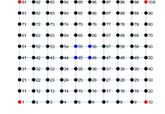
We consider the two scenarios presented in Fig. 4:
-
-
Scenario 1 (Dispersed Support): In this scenario, the signal support set is located on the edges of the square grid graph. For the considered -node square grid graph, the node positions are (shown in red in Fig. 4). This scenario describes a situation where the locations of the non-zero elements of the sparse signal are far apart across the graph.
-
-
Scenario 2 (Localized Support): In this scenario, the support set of the signal is concentrated in neighboring nodes (here, in the center of the square grid graph). For the considering -node square grid graph, the node positions are ) (shown in blue in Fig. 4). This scenario describes a situation where the non-zero elements are clustered in close proximity within the graph structure.
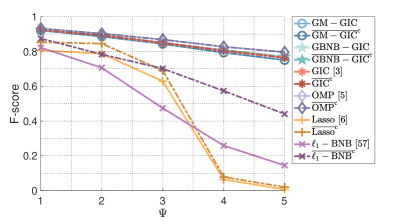
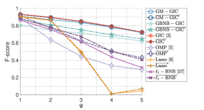
The F-score results for Scenario 1 and Scenario 2 are presented in Figs. 5.a and 5.b, respectively, versus the graph filter degree. Figure 5.a shows that for Scenario 1, the F-score for the GM-GIC, G-BNB, and OMP methods is similar for any graph filter degree and achieves the benchmark score of the GIC method. This can be explained by the fact that a dispersed support set is easy to recover. Additionally, the F-score decreases moderately as the graph filter degree increases (from to ). In contrast, the F-score of the Lasso and the -BNB methods significantly decreases as the graph filter degree increases (e.g. the F-score of the -BNB method ranges from to ). For this case, the proposed GFOC method significantly improves the -BNB method’s F-score for any graph filter degree, and improves the F-score of the Lasso method for . Figure 5.b shows that for Scenario 2 of the localized support, only the GM-GIC achieves F-scores comparable to the optimal GIC method. The G-BNB method is the closest behind, with F-scores lower by at most . The corrected version method performs even better, with F-scores lower than those of the GM-GIC method by at most . The Lasso method obtains equivalent results to the GM-GIC method for , but provides poor results for graph filter degrees larger than . Both the OMP and -BNB methods exhibit a significant decrease in F-score as the graph filter degree increases. Finally, the improvement obtained by the proposed GFOC method is the most significant when applied to the OMP technique.
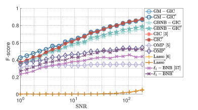
Figure 6 presents the F-score versus the SNR for Scenario 2, where the graph filter degree is set to . In this scenario, the GIC, GM-GIC, and G-BNB methods have the highest F-scores (ranging from approximately to ), which increases as the SNR increases. The corrected version of the OMP method, , improves the OMP F-score by about , compared to the original OMP. Additionally, the corrected versions of the -BNB, and methods show similar results to those from the method for high SNRs. The Lasso method and its corrected version show poor results across all observed SNRs.
VI-B2 Case 2- Erdős Réyni Graph with Nodes
We consider the graph in Fig. 7, which is a realization of an Erdős-Rényi graph with the probability of that two nodes are connected. The signal support set has been selected uniformly from the following two cases:
-
-
Scenario 3 (Mixed Dispersed-Localized Support): In this scenario, two groups of two nodes are selected as follows. First, two nodes are selected at random from the Erdős Réyni graph in Fig. 7. Then, for each node, one of its neighbors is randomly chosen and added to the support set. This process is repeated until four different nodes are selected. This scenario describes a situation where the non-zero elements are clustered in two distanced groups, where the nodes in each group are in close proximity.
-
-
Scenario 4 (Localized Support): In this scenario, a single node is randomly selected from the Erdős Réyni graph in Fig. 7. Then, three of the node’s neighbors are randomly chosen and added to the support set. This scenario describes a situation where the non-zero elements are clustered in close proximity within the graph structure.
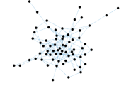
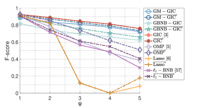
Figure 8 shows the F-score as a function of the graph filter degree, where is drawn from Scenario and Scenario with equal probability. Unlike the results in Fig. 5, none of the methods show similar results to the optimal GIC method. The GM-GIC and its correction methods obtain the closest result. Closely behind is the method, with results up to better than the G-BNB method. The method shows similar results to the method for the first graph degrees, yet lower F-scores at the higher degrees. The Lasso and -BNB methods and their corrections show competitive results only for the first graph degrees.
VI-C Run-Time
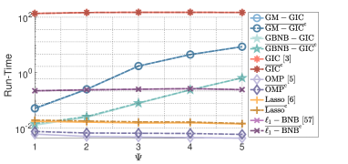
In order to demonstrate the computational complexity of the different methods empirically, their associated run-time (average computation time) is evaluated using Matlab on two Intel(R) Xeon(R) CPU E5-2660 v4 @ 2.00 GHz processors. The signal support set, , in the following simulation is drawn with equal probability from Scenario and Scenario . In Fig. 9(a), we present the run-time of the different algorithms versus the graph filter degree. The optimal GIC method requires the highest run-time (operating in close to seconds). The run-time of the GM-GIC and G-BNB methods increases as the graph filter degree increases, where the GM-GIC method run-time is substantially larger than the G-BNB method run time. For example, for , the GM-GIC method requires a couple of seconds while the G-BNB method operates in milliseconds. The G-BNB method requires a lower run-time than the -BNB method for the first graph filter degrees. The Lasso and OMP methods perform the fastest; however, as shown in Figs. 5, 6, and 8, these methods display lower F-scores in comparison to the proposed methods. Notably, the additional run-time required by the GFOC method to correct these methods is negligible for all the methods.
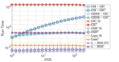
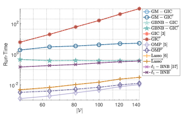
In Fig. 9(b), we present the run-time versus the SNR where the graph filter degree is . It can be seen that the run-time of the GM-GIC method significantly increases as the SNR increases. The run-time required for the remaining methods is constant w.r.t. the SNR. The G-BNB method requires a significantly lower run-time than the GM-GIC method and yields similar results to the -BNB methods. Figure 9(c) presents the run-time as a function of the graph size, where the filter degree is and the signal support set, , is chosen with equal probability from Scenarios and . The run-time required for the optimal GIC methods grows exponentially with the graph (model) size. In contrast, the GM-GIC is only slightly affected, while the G-BNB run-time is constant across the different graph sizes. The graph size also affects the Lasso and OMP methods, but both still operate significantly faster than the other methods.
VII Conclusions
In this paper, we propose three sparse recovery techniques: the GM-GIC, Graph-BNB-GIC, and GFOC methods. These techniques solve the support set recovery problem for diffused sparse graph signals, which are node-domain sparse graph signals diffused over the graph by a graph filter. The proposed methods use the GIC as the optimization cost function and leverage the underlying graphical structure to reduce the computational complexity and enhance the recovery performance. In particular, the GM-GIC and Graph-BNB-GIC directly tackle the support set recovery problem by considering local graph properties and efficiently partitioning the dictionary elements and iteratively searching over candidate support sets, respectively. The GFOC method is based on correcting the solution obtained by any other support set recovery technique. In addition, we provide a theoretical analysis of the considered setting with: 1) an examination of the dictionary matrix atoms (i.e. graph filter columns) derived from the underlying graphical structure; and 2) an evaluation of the computational complexity of the proposed methods, based on the graph filter degree, the maximum degree of the graph, and sparsity restrictions. Simulations conducted over the square grid graph and the Erdős-Rényi graph reveal that our proposed GM-GIC and Graph-BNB-GIC methods achieve higher support set recovery accuracy compared to state-of-the-art methods such as OMP, Lasso, and -BNB, while maintaining significantly lower computational overhead than the optimal GIC method. In general, the GM-GIC method outperforms the Graph-BNB-GIC method in terms of the accuracy of the support set recovery, but requires more computing time. It is also demonstrated that the GFOC method can significantly improve the support set recovery accuracy of existing methods, including the OMP, Lasso, and -BNB methods, without imposing significant additional computation overhead. By applying the GFOC method on the Graph-BNB-GIC method, we obtained support set estimation results comparable to the GIC benchmark, with a run-time comparable to the OMP and Lasso methods. Consequently, the best performance is obtained by combining the Graph-BNB-GIC and GFOC methods.
References
- [1] G. Morgenstern and T. Routtenberg, “Sparse graph signal recovery by the graph-based multiple generalized information criterion (GM-GIC),” in International Workshop on Computational Advances in Multi-Sensor Adaptive Processing (CAMSAP), 2023, pp. 491–495.
- [2] A. Ortega, P. Frossard, J. Kovačević, J. M. Moura, and P. Vandergheynst, “Graph signal processing: Overview, challenges, and applications,” Proc. IEEE, vol. 106, no. 5, pp. 808–828, 2018.
- [3] D. I. Shuman, S. K. Narang, P. Frossard, A. Ortega, and P. Vandergheynst, “The emerging field of signal processing on graphs: Extending high-dimensional data analysis to networks and other irregular domains,” IEEE Signal Process. Mag., vol. 30, no. 3, pp. 83–98, 2013.
- [4] A. Sandryhaila and J. M. Moura, “Discrete signal processing on graphs,” IEEE Trans. Signal Process., vol. 61, no. 7, pp. 1644–1656, 2013.
- [5] ——, “Discrete signal processing on graphs: Frequency analysis,” IEEE Trans. Signal Process., vol. 62, no. 12, pp. 3042–3054, 2014.
- [6] A. G. Marques, S. Segarra, G. Leus, and A. Ribeiro, “Stationary graph processes and spectral estimation,” IEEE Trans. Signal Process., vol. 65, no. 22, pp. 5911–5926, 2017.
- [7] E. Drayer and T. Routtenberg, “Detection of false data injection attacks in smart grids based on graph signal processing,” IEEE Syst. J., vol. 14, no. 2, pp. 1886–1896, 2019.
- [8] Y. Tanaka, Y. C. Eldar, A. Ortega, and G. Cheung, “Sampling signals on graphs: From theory to applications,” IEEE Signal Process. Mag., vol. 37, no. 6, pp. 14–30, 2020.
- [9] A. G. Marques, S. Segarra, G. Leus, and A. Ribeiro, “Sampling of graph signals with successive local aggregations,” IEEE Trans. Signal Process., vol. 64, no. 7, pp. 1832–1843, 2015.
- [10] S. Chen, A. Sandryhaila, J. M. Moura, and J. Kovačević, “Signal recovery on graphs: Variation minimization,” IEEE Trans. Signal Process., vol. 63, no. 17, pp. 4609–4624, 2015.
- [11] P. Di Lorenzo, P. Banelli, E. Isufi, S. Barbarossa, and G. Leus, “Adaptive graph signal processing: Algorithms and optimal sampling strategies,” IEEE Trans. Signal Process., vol. 66, no. 13, pp. 3584–3598, 2018.
- [12] G. Sagi and T. Routtenberg, “MAP estimation of graph signals,” IEEE Trans. Signal Process., vol. 72, pp. 463–479, 2024.
- [13] A. Kroizer, T. Routtenberg, and Y. C. Eldar, “Bayesian estimation of graph signals,” IEEE Trans. Signal Process., vol. 70, pp. 2207–2223, 2022.
- [14] A. Amar and T. Routtenberg, “Widely-linear mmse estimation of complex-valued graph signals,” IEEE Trans. Signal Process., vol. 71, pp. 1770–1785, 2023.
- [15] L. Dabush and T. Routtenberg, “Verifying the smoothness of graph signals: A graph signal processing approach,” arXiv preprint: 2307.03210, 2023.
- [16] A. Venkitaraman, S. Chatterjee, and P. Händel, “Predicting graph signals using kernel regression where the input signal is agnostic to a graph,” IEEE Trans. Signal Inf. Process. Netw., vol. 5, no. 4, pp. 698–710, 2019.
- [17] E. Isufi, A. Loukas, A. Simonetto, and G. Leus, “Autoregressive moving average graph filtering,” IEEE Trans. Signal Process., vol. 65, no. 2, pp. 274–288, 2016.
- [18] M. Coutino, E. Isufi, and G. Leus, “Advances in distributed graph filtering,” IEEE Trans. Signal Process., vol. 67, no. 9, pp. 2320–2333, 2019.
- [19] S. S. Chen, D. L. Donoho, and M. A. Saunders, “Atomic decomposition by basis pursuit,” SIAM Review, vol. 43, no. 1, pp. 129–159, 2001.
- [20] J. A. Tropp, “Greed is good: algorithmic results for sparse approximation,” IEEE Trans. Inf. Theory, vol. 50, no. 10, pp. 2231–2242, Oct. 2004.
- [21] D. L. Donoho, M. Elad, and V. N. Temlyakov, “Stable recovery of sparse overcomplete representations in the presence of noise,” IEEE Trans. Inf. Theory, vol. 52, no. 1, pp. 6–18, 2005.
- [22] M. Elad, Sparse and Redundant Representations: From Theory to Applications in Signal and Image Processing. New York, NY, USA: Springer Science & Business Media, 2010.
- [23] R. Tibshirani, “Regression shrinkage and selection via the lasso,” Journal of the Royal Statistical Society Series B: Statistical Methodology, vol. 58, no. 1, pp. 267–288, 1996.
- [24] B. Efron, T. Hastie, I. Johnstone, and R. Tibshirani, “Least angle regression,” The Annals of Statistics, vol. 32, no. 2, pp. 407 – 499, 2004.
- [25] E. Candes and T. Tao, “The dantzig selector: Statistical estimation when p is much larger than n,” The Annals of Statistics, vol. 35, no. 6, pp. 2313 – 2351, 2007.
- [26] D. L. Donoho, A. Maleki, and A. Montanari, “Message-passing algorithms for compressed sensing,” Proceedings of the National Academy of Sciences, vol. 106, no. 45, pp. 18 914–18 919, 2009.
- [27] D. P. Wipf and B. D. Rao, “Sparse bayesian learning for basis selection,” IEEE Trans. Signal Process., vol. 52, no. 8, pp. 2153–2164, 2004.
- [28] I. F. Gorodnitsky and B. D. Rao, “Sparse signal reconstruction from limited data using focuss: A re-weighted minimum norm algorithm,” IEEE Trans. Signal Process., vol. 45, no. 3, pp. 600–616, 1997.
- [29] R. Chartrand and W. Yin, “Iteratively reweighted algorithms for compressive sensing,” in International Conference on Acoustics, Speech and Signal Processing (ICASSP). IEEE, 2008, pp. 3869–3872.
- [30] S. G. Mallat and Z. Zhang, “Matching pursuits with time-frequency dictionaries,” IEEE Trans. Signal Process., vol. 41, no. 12, pp. 3397–3415, 1993.
- [31] T. T. Cai and L. Wang, “Orthogonal matching pursuit for sparse signal recovery with noise,” IEEE Trans. Inf. Theory, vol. 57, no. 7, pp. 4680–4688, 2011.
- [32] W. Dai and O. Milenkovic, “Subspace pursuit for compressive sensing signal reconstruction,” IEEE Trans. Inf. Theory, vol. 55, no. 5, pp. 2230–2249, 2009.
- [33] T. Blumensath and M. E. Davies, “Gradient pursuits,” IEEE Trans. Signal Process., vol. 56, no. 6, pp. 2370–2382, 2008.
- [34] J. Haupt, W. U. Bajwa, M. Rabbat, and R. Nowak, “Compressed sensing for networked data,” IEEE Signal Process. Mag., vol. 25, no. 2, pp. 92–101, 2008.
- [35] W. Xu, E. Mallada, and A. Tang, “Compressive sensing over graphs,” in 2011 Proceedings IEEE INFOCOM. IEEE, 2011, pp. 2087–2095.
- [36] M. Cheraghchi, A. Karbasi, S. Mohajer, and V. Saligrama, “Graph-constrained group testing,” IEEE Trans. Inf. Theory, vol. 58, no. 1, pp. 248–262, 2012.
- [37] P. C. Pinto, P. Thiran, and M. Vetterli, “Locating the source of diffusion in large-scale networks,” Physical review letters, vol. 109, no. 6, p. 068702, 2012.
- [38] E. Sefer and C. Kingsford, “Diffusion archeology for diffusion progression history reconstruction,” Knowledge and information systems, vol. 49, pp. 403–427, 2016.
- [39] P. Zhang, J. He, G. Long, G. Huang, and C. Zhang, “Towards anomalous diffusion sources detection in a large network,” ACM Transactions on Internet Technology (TOIT), vol. 16, no. 1, pp. 1–24, 2016.
- [40] R. Pena, X. Bresson, and P. Vandergheynst, “Source localization on graphs via 1 recovery and spectral graph theory,” in Image, Video, and Multidimensional Signal Processing Workshop (IVMSP), 2016, pp. 1–5.
- [41] A. Sridhar, T. Routtenberg, and H. V. Poor, “Quickest inference of susceptible-infected cascades in sparse networks,” in International Symposium on Information Theory (ISIT), 2023, pp. 102–107.
- [42] A. Anis, A. Gadde, and A. Ortega, “Towards a sampling theorem for signals on arbitrary graphs,” in International Conference on Acoustics, Speech and Signal Processing (ICASSP), 2014, pp. 3864–3868.
- [43] S. Chen, R. Varma, A. Sandryhaila, and J. Kovacevic, “Discrete signal processing on graphs: Sampling theory,” IEEE Trans. Signal Process., vol. 63, no. 24, pp. 6510–6523, 2015.
- [44] M. Tsitsvero, S. Barbarossa, and P. Di Lorenzo, “Signals on graphs: Uncertainty principle and sampling,” IEEE Trans. Signal Process., vol. 64, no. 18, pp. 4845–4860, 2016.
- [45] D. Ramírez, A. G. Marques, and S. Segarra, “Graph-signal reconstruction and blind deconvolution for structured inputs,” Signal Process., vol. 188, p. 108180, 2021.
- [46] S. Segarra, G. Mateos, A. G. Marques, and A. Ribeiro, “Blind identification of graph filters,” IEEE Trans. Signal Process., vol. 65, no. 5, pp. 1146–1159, 2016.
- [47] S. Segarra, A. G. Marques, and A. Ribeiro, “Optimal graph-filter design and applications to distributed linear network operators,” IEEE Trans. Signal Process., vol. 65, no. 15, pp. 4117–4131, 2017.
- [48] ——, “Distributed implementation of linear network operators using graph filters,” in Annual Allerton Conference on Communication, Control, and Computing (Allerton), 2015, pp. 1406–1413.
- [49] J. Mei and J. M. Moura, “Signal processing on graphs: Estimating the structure of a graph,” in International Conference on Acoustics, Speech and Signal Processing (ICASSP), 2015, pp. 5495–5499.
- [50] H. Rainer and U. Krause, “Opinion dynamics and bounded confidence: Models, analysis and simulation,” Journal of Artificial Societies and Social Simulation, vol. 5, no. 3, 2002.
- [51] D. Shah and T. Zaman, “Rumors in a network: Who’s the culprit?” IEEE Trans. Inf. Theory, vol. 57, no. 8, pp. 5163–5181, 2011.
- [52] M. E. Newman, “Spread of epidemic disease on networks,” Physical review E, vol. 66, no. 1, p. 016128, 2002.
- [53] D. Shah and T. Zaman, “Detecting sources of computer viruses in networks: theory and experiment,” in Proceedings of the ACM SIGMETRICS international conference on Measurement and modeling of computer systems, 2010, pp. 203–214.
- [54] G. Morgenstern and T. Routtenberg, “Structural-constrained methods for the identification of unobservable false data injection attacks in power systems,” IEEE Access, vol. 10, pp. 94 169–94 185, 2022.
- [55] G. Morgenstern, J. Kim, J. Anderson, G. Zussman, and T. Routtenberg, “Protection against graph-based false data injection attacks on power systems,” IEEE Trans. Control Netw. Syst., pp. 1–12, 2024.
- [56] S. Segarra, A. G. Marques, G. Leus, and A. Ribeiro, “Reconstruction of graph signals through percolation from seeding nodes,” IEEE Trans. Signal Process., vol. 64, no. 16, pp. 4363–4378, 2016.
- [57] Y. Zhu, F. J. I. Garcia, A. G. Marques, and S. Segarra, “Estimating network processes via blind identification of multiple graph filters,” IEEE Trans. Signal Process., vol. 68, pp. 3049–3063, 2020.
- [58] C. Ye, R. Shafipour, and G. Mateos, “Blind identification of invertible graph filters with multiple sparse inputs,” in European Signal Processing Conference (EUSIPCO), 2018, pp. 121–125.
- [59] S. Rey-Escudero, F. J. I. Garcia, C. Cabrera, and A. G. Marques, “Sampling and reconstruction of diffused sparse graph signals from successive local aggregations,” IEEE Signal Process. Lett., vol. 26, no. 8, pp. 1142–1146, 2019.
- [60] S. Boyd and J. Mattingley, “Branch and bound methods,” Notes for EE364b, Stanford University, vol. 2006, p. 07, 2007.
- [61] E. L. Lawler and D. E. Wood, “Branch-and-bound methods: A survey,” Operations research, vol. 14, no. 4, pp. 699–719, 1966.
- [62] Z. Wang, A. Scaglione, and R. J. Thomas, “Generating statistically correct random topologies for testing smart grid communication and control networks,” IEEE Trans. Smart Grid, vol. 1, no. 1, pp. 28–39, 2010.
- [63] S. M. Kay, Fundamentals of statistical signal processing: Estimation Theory. New Jersey, NJ, USA: Prentice Hall PTR, 1993, vol. 1.
- [64] H. Yanai, K. Takeuchi, and Y. Takane, “Projection matrices,” in Projection Matrices, Generalized Inverse Matrices, and Singular Value Decomposition. Springer, 2011, pp. 25–54.
- [65] P. Babu and P. Stoica, “Multiple-hypothesis testing rules for high-dimensional model selection and sparse-parameter estimation,” Signal Process., vol. 213, p. 109189, 2023.
- [66] P. Stoica and Y. Selen, “Model-order selection: a review of information criterion rules,” IEEE Signal Process. Mag., vol. 21, no. 4, pp. 36–47, 2004.
- [67] S. M. Kay, Fundamentals of Statistical Signal Processing, Volume II: Detection Theory. New Jersey, NJ, USA: Prentice Hall PTR, 1993.
- [68] R. Dionne and M. Florian, “Exact and approximate algorithms for optimal network design,” Networks, vol. 9, no. 1, pp. 37–59, 1979.
- [69] R. S. Solanki, J. K. Gorti, and F. Southworth, “Using decomposition in large-scale highway network design with a quasi-optimization heuristic,” Transportation Research Part B: Methodological, vol. 32, no. 2, pp. 127–140, 1998.
- [70] B. Bollobás, “Random graphs,” in Modern Graph Theory. New York, NY, USA: Springer, 1998, pp. 215–252.
- [71] M. Sokolova and G. Lapalme, “A systematic analysis of performance measures for classification tasks,” Information Processing and Management, vol. 45, pp. 427–437, 07 2009.