A Deep Learning Approach to Heterogeneous Consumer Aesthetics in Retail Fashion

Abstract

In some markets, the visual appearance of a product matters a lot. This paper investigates consumer transactions from a major fashion retailer, focusing on consumer aesthetics. Pretrained multimodal models convert images and text descriptions into high-dimensional embeddings. The value of these embeddings is verified both empirically and by their ability to segment the product space. A discrete choice model is used to decompose the distinct drivers of consumer choice: price, visual aesthetics, descriptive details, and seasonal variations. Consumers are allowed to differ in their preferences over these factors, both through observed variation in demographics and allowing for unobserved types. Estimation and inference employ automatic differentiation and GPUs, making it scalable and portable. The model reveals significant differences in price sensitivity and aesthetic preferences across consumers. The model is validated by its ability to predict the relative success of new designs and purchase patterns.

Keywords Image Processing  $\cdot$ Consumer Choice  $\cdot$ Deep Learning

1 Introduction

In some industries, visual appeal is extremely important. This includes markets such as fashion, interior, watches, jewelry, art, movies, and TV. There are many visual elements, such as color, shape, size, texture, pattern, reflectivity, cut, style, proportion, or ornamentation, that give visual appeal to the product. The way in which the product is being presented to the customer—either over the internet or in real life—will also bear on the aesthetics of the image. This includes size, quality, lighting, contrast, framing, and bordering of the image. What appeals to some may not appeal to others, and there is an array of attributes that may be regarded well by some but not by others. This project aims to quantify aesthetic attractiveness by isolating those elements in high-resolution images of products. The focus is to measure how "beauty is to the eyes of the beholder" and how different sections of consumers have different aesthetic tastes. This project uses a transactional dataset from fashion retailer H&M to demonstrate a methodology that can capture heterogeneous consumer aesthetics.

Images are a valuable source of information for many reasons. First, consumers are drawn to them and almost never purchase without looking at the image. That alone makes images important. Second, in those industries where visual elements matter, images can help us estimate how sensitive consumers are to price changes by controlling for those visual factors. They can also be used to build instruments to account for unobserved confounders. Lastly, images are interesting in their own right. By analyzing them, we can gain insights into the aesthetic preferences of different groups of people and leverage this knowledge to develop and test new designs. This is a very important question for retail fashion firms like H&M to answer, for their entire business model revolves around understanding “trends" and bringing trendy designs to consumers as soon as possible. Retrospectively, with image data on old products, we could ask questions about how well firms like H&M are able to supply aesthetic designs that are desired by people.

Having established the importance of images, I define the research agenda. The research questions of this project are: Firstly, how do we extract product aesthetics from an image? This is a technical problem of representation, and I draw models from deep learning that help us solve this task. I validate this procedure, showing that not only do these deep learning techniques help us extract information from images, but the information captured is intuitive and can be visualized. Secondly, how can we capture a diversity of aesthetic tastes across consumers? This is a question about the best way to model the interaction between consumer demographics and the representation of the image. The discrete choice/brand choice framework is chosen as appropriate for this task, and another layer of machine learning methods is selected as the best way to operate on high dimensional covariates and demographics. The model is validated by testing its predictions on data and aesthetic designs it has not seen. Lastly, how can we develop and test new aesthetic designs? This is a question about informal hypothesis testing, and a simple simulation-based approach is selected to help us predict how different demographics do on different aesthetic designs.

2 Literature Review

The extended literature relevant to this study spans several domains, integrating works on demand/choice models by Train (2009), Gandhi and Houde (2019), Conlon and Gortmaker (2020), Berry and Haile (2021), and Petrin and Train (2010). Additionally, this project considers advancements in deep learning architectures, as illustrated by contributions from Younesi et al. (2024), Vaswani et al. (2017), known for the transformer model, Kingma et al. (2015), who introduced variational autoencoders, LeCun et al. (2015), He et al. (2016) with the inception of residual networks, and Sun et al. (2020). The intersection of machine learning with econometrics is also critical, highlighted by the works of Chernozhukov et al. (2018, 2022), Farrell et al. (2018, 2021), and Ludwig and Mullainathan (2023). Moreover, specific studies related to the retail fashion industry by McCormick et al. (2014), Wen et al. (2019), and Bhardwaj and Fairhurst (2009) provide insights into market dynamics and consumer behavior. Applied works further contextualize the practical applications of these theories and methodologies, including those by Quah & Williams (2021), Han et al. (2021), Giovanni et al. (2021), Zhang et al. (2022), He et al. (2023), Janssens et al. (2021), and Zhang (2024), each adding unique perspectives and findings to the body of knowledge this project builds on.

I now review the applied papers that are most relevant to this study. Quah & Williams (2021) represent product images in high-dimensional embeddings and apply debiased machine learning techniques to estimate the market demand for shoes accurately. Their work showcases the power of image data in building controls and instruments for market demand estimation. Giovanni et al. (2021) focus on the similarity scores between product pages on Amazon and utilize this information to model error covariances within a nested logit framework. They highlight the use of high-dimensional data to model unobservables. Han et al. (2021) explore using dense embeddings derived from image autoencoders to estimate demand for various font styles. They also show how image embeddings help segment the product space. Magnolfi et al. (2022) use consumer survey data to construct embeddings from data on cereal product comparisons. They find that their method helps them get more realistic estimates of price sensitivity. Zhang (2024) employs deep neural networks to model heterogeneous price sensitivities in a model of consumer choice. A recurrent neural network is used to model online browsing activity, and that is used to segment users. Finally, Dubé and Misra, 2023) estimate a model of heterogeneous consumer choice and use it for personalized pricing. These studies collectively showcase the increasing prominence of high-dimensional data, particularly images and text, in estimating price sensitivity and understanding consumer behavior.

This research also draws from a couple of methodological papers. Chernozhukov et al. (2018, 2022) emphasize the importance of sample-splitting techniques in reducing regularization bias when using regularized machine learning methods. Farrell et al. (2018, 2021) demonstrate the power of neural networks in estimating parameter functions. They prove that neural networks converge fast enough for inference to be conducted and apply their method to estimate heterogeneous choice models and optimize discounting policies. Berry and Haile (2021) and Train (2009) provide comprehensive surveys on demand and choice models. Ludwig and Mullainathan (2023) explore the use of machine learning for hypothesis generation in economic research. They use convolutional neural networks on mugshots to reveal the presence of bias in judicial decisions. These methodological advances have inspired much interest in estimation with high dimensional covariates.

While existing methods offer valuable tools for analyzing consumer behavior, they often fall short of addressing the specific goals of this research. First is a limited consideration of individual heterogeneity. Many existing models fail to capture the unique preferences of individual consumers. Secondly, even considering individual differences, existing methods often prioritize price sensitivity. While price sensitivity is critical in merger analysis and demand estimation, this project has a different focus - heterogeneous consumer aesthetic taste. The main contribution of this project is about modeling variation in aesthetic taste. While aesthetics is a primary focus, I acknowledge the influence of other variables like price, fabric, and seasonal factors. These factors are incorporated as controls within our model. This project also uses automatic differentiation, deep learning, and advancements in computational resources (GPUs) to build a scalable and portable model of brand choice.

So far, I have not come across other research that does two things that this project does. First, amongst the literature that uses machine learning methods in an econometric framework – this project is the first to use multi-modal models that combine two different sources of unstructured data (images and text). Secondly, this paper is the first to combine these unstructured data with rich demographic data. This allows us to get a unique insight into what different demographics prefer. In this way, this project hopes to contribute something new to the field.

3 Retail Fashion Industry

The retail fashion industry is characterized by monopolistic competition—many small to medium firms, differentiated products, and few entry barriers. It has a large number of incomparable products with short product lifespans. There are many seasonal products and distinct collections with a non-replenishable inventory. Promotions and discounts are also widely used. Some brands garner some loyalty, while most others do not. Retailers have more market power than suppliers because suppliers are many and spread across the globe, while retailers are few and found primarily in rich advanced economies. Entry and exit barriers are few - one can simply note how many celebrities attempt to start their own brands - and so there is intense competition. Due to the homogeneity of products, there is sharp competition in prices, but some retailers (notably Zara and H&M) are able to differentiate themselves by offering a unified omnichannel (store-website-app) experience and superior supply chain responsiveness.

The retail fashion industry has undergone significant transformations since the 1980s (Bhardwaj and Fairhurst 2009). Several factors, including shifts in product design, fashion seasons, supply chain operations, and consumer behavior, have driven these changes. The industry has moved from mass-producing staple items such as Levi’s 501 and white tees to more trendy and stylish clothing. However, this shift has also increased mark-downs due to excess inventory and failure to sell products during the season. One notable change in the industry is the shrinking time between runway shows and product delivery, with the incorporation of 3-6 mid-seasons to the traditional fashion calendar (Spring/Summer/Autumn/Winter). This helped reduce lead times. Quick Response and Just-in-Time strategies have also been developed to improve efficiency. There has also been a decisive shift to outsourcing as firms looked to cut costs by employing labor from poorer countries. Finally, consumers have become more fashion-conscious and price-sensitive, demanding cheaper yet fashionable clothes.

These changes meant that retailers increasingly prioritized low cost, design flexibility, and speed to market (Djelic & Ainamo, 1999). This evolution has given rise to fast fashion, exemplified by retailers like Zara and H&M, who offer frequent updates to meet consumer demand for variety and instant gratification (Sydney, 2008). Around 1999, fashion runways and shows transitioned from exclusive events to public spectacles, exposing consumers to runway designs and inspiring rapid adaptation by retailers like Zara and H&M (Barnes & Lea-Greenwood, 2006). The emergence of fast fashion signifies a shift from forecasting future trends to using real-time data to understand consumer preferences (Jackson, 2001). In the UK, retailers like New Look and George pioneered practices like just-in-time manufacturing and quick response to maintain competitiveness (Bruce et al., 2004).

Ferdows et al. (2014) provide deep insights into the Zara model. Insights from the market leader Zara highlight a remarkable trajectory from its modest start to becoming the world’s largest apparel company, characterized by strategic rapid expansion and effective market penetration. From 2001 to 2014, Zara’s store count surged from 1,284 in 39 countries to 6,683 across 88 countries. Central to Zara’s success is its agile supply chain management, enabling the brand to design, produce, and distribute clothing within two weeks, contrasting sharply with the several-month cycle typical within the industry. This capability underscores a management philosophy rooted in simplicity and empowerment across all employee levels, facilitating swift decision-making essential for keeping pace with rapidly changing fashion trends. Technologically, Zara integrates advanced data analytics to dynamically forecast demand and adjust supply strategies, ensuring precise anticipation and responsiveness to global fashion trends. Trying to keep up with social trends and sustainability, Zara has been responding to consumers who urge ethical fashion with various sustainability strategies. Finally, Zara’s business model allows the company to receive sales cash quicker than it does when paying suppliers. It supports self-financed expansions and also sustains growth even during economic downturns.

Over the years, technological advancements have changed the fashion retail industry. Firstly, there is the development of omnichannel retailing. Omnichannel retail is an approach to retailing that streamlines physical stores, online platforms, and mobile apps to provide a unified shopping experience. Secondly, frequent promotions and dynamic pricing allow rapid adjustment to market demand and customer willingness to pay. Thirdly, RFID tags in supply chains have reduced inventory errors and improved stock accuracy, facilitating quicker restocking and minimizing out-of-stock situations. Fourthly, advanced optimization routines like mixed integer programming optimize production scheduling and pricing, aligning production with demand fluctuations to prevent overproduction and boost profitability. Lastly, sustainability practices are rising, with initiatives like garment recycling systems enhancing brands’ environmental responsibility.

The next generation of AI is poised to advance retail fashion in many ways. In product development, AI can analyze unstructured data from social media and other sources to detect trends and sentiment. Generative AI can create diverse design options and utilize facial recognition to customize products such as eyeglasses. In customer support, chatbots with advanced natural-language processing improve interactions. These chatbots handle multilingual, complex queries and reduce response times. Continuous communication can improve clienteling, and virtual try-ons help improve the shopping experience. Retrieval augmented generation can help customers make sense of reviews, comments, and product details. In marketing, AI can help teams quickly develop strategies and content and generate viral videos for platforms like TikTok, reducing time and cost. In logistics, robotic automation is likely to improve warehouse operations and distribution.

4 Data

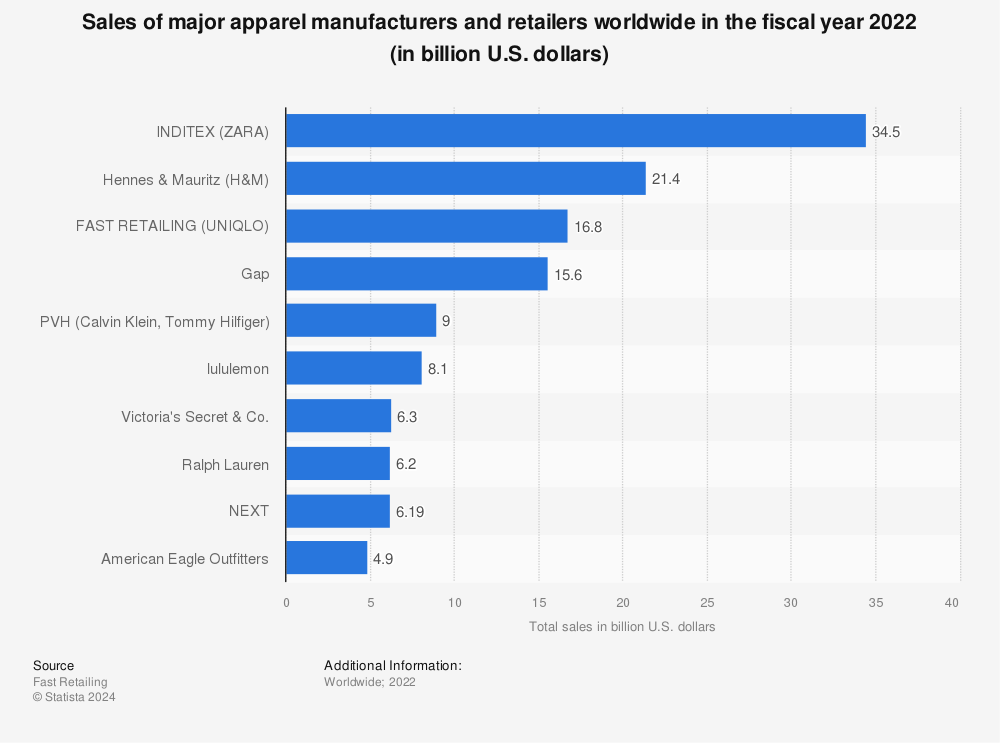
Figure 4: Share of Items in Shopping Day

The data used for this project was released by Hennes & Mauritz (H&M), a leading Swedish fast fashion company. H&M operates in 75 different geographic markets, boasting 4,800 stores worldwide and approximately 107,000 employees. The company’s annual revenue amounts to 24.8 billion USD. H&M’s core mission revolves around making fashion accessible and enjoyable for everyone, with designs featured on runways, swiftly making their way to stores worldwide within two weeks, all at affordable prices. However, the brand is often associated with low-quality construction and product variability, with some items showing signs of wear and tear after minimal use. H&M faces stiff competition from other fast fashion retailers such as Zara, Gap, and Uniqlo. Regarding market share, H&M is only behind Zara and ahead of Uniqlo and Gap (see Figure 4).

The dataset consists of a subset of two years of shopping transactions conducted at H&M, involving a large customer base of 1,371,980 individuals. The median age of customers is 32, with around 66% classified as active. Additionally, the dataset contains a significant inventory of 108,775,015 Stock Keeping Units (SKUs), including various categories such as Ladieswear (25%), Divided (14%), and Menswear (12%). Women’s Dresses emerge as a popular category among these SKUs, with a diverse range of products totaling 2,300 distinct SKUs. Transaction data amount to 31,788,324 instances, with 70% occurring offline and 30% online, illustrating the significant digital footprint of the company alongside traditional retail. Furthermore, the dataset includes 45,875 unique product names and 43,404 text descriptions, providing comprehensive information for analysis and modeling.

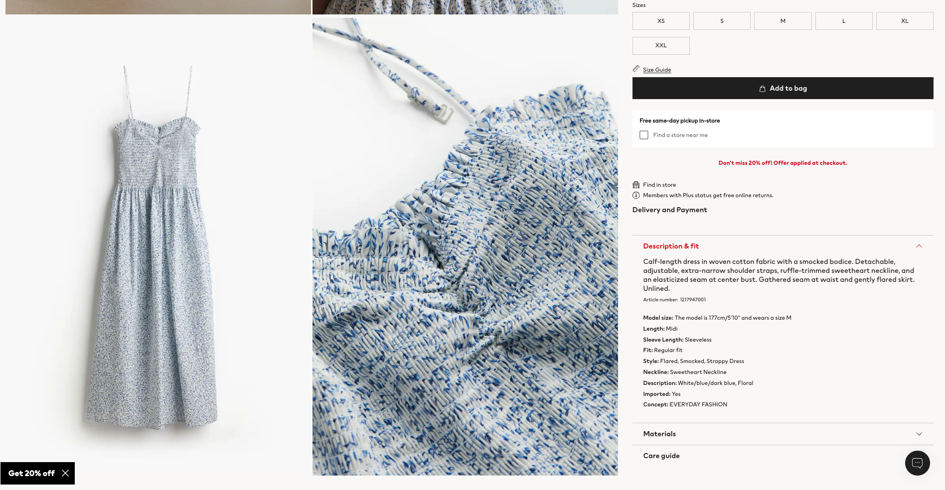
Figure 5: The product page at H&M’s Website

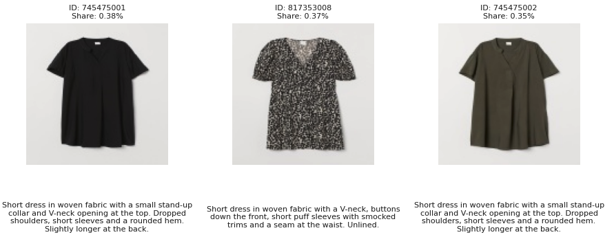
Figure 6: The Best Selling Products

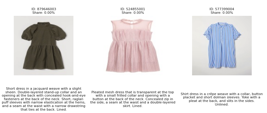
Figure 7: Some Worst Selling Products

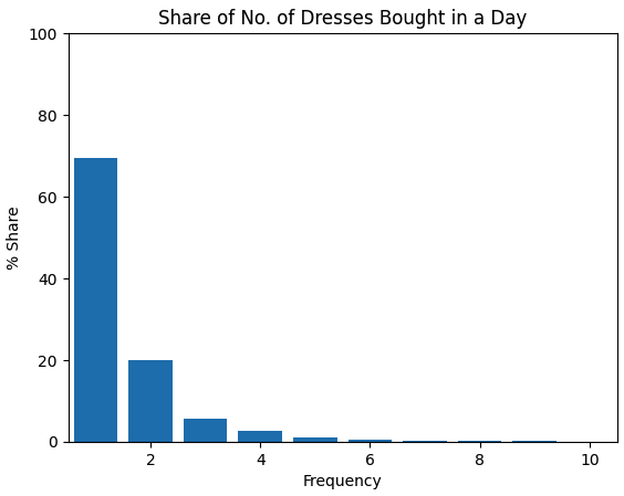
Figure 8: Share of Number of Dresses Purchased in a Shopping-Day

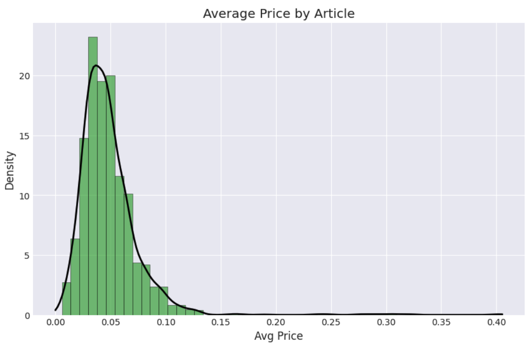
Figure 9: Kernel Density and Distribution of Avg Prices

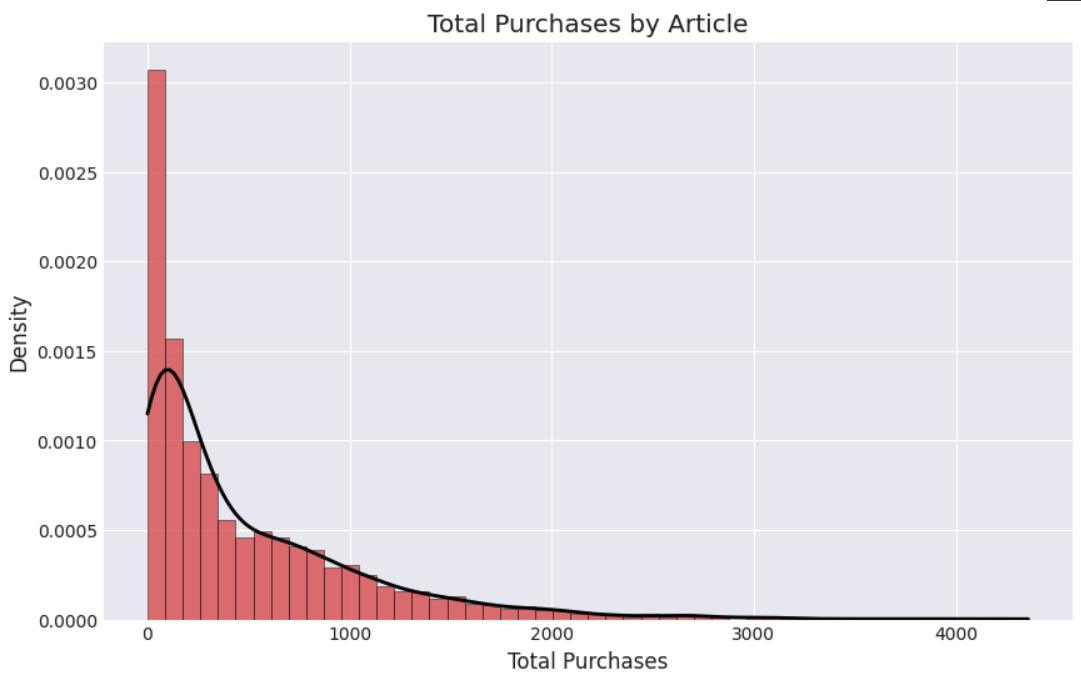
Figure 10: Kernel Density and Distribution of Sales Share

My data on dress purchases includes clear product images with detailed descriptions (see Figures 5, 6, and 7). Interestingly, most shoppers only buy one article in a single shopping day (Figure 8). That fact suggests that a discrete choice framework is suitable for analyzing this data, where individuals pick one choice from a set of options in a given shopping session. Sales data reveals seasonal solid trends (see Figures 11 to 15), with a few dresses generating the majority of sales (highly skewed distribution), reflecting the fast fashion industry’s reliance on a few trending items to drive substantial portions of revenue (Figure 9). We also see significant price fluctuations with sharp discounting and a bell-shaped price distribution over time (Figure 10).

The comparative advantage of this data is that it is the only open-source data I know of that contains (1) granular consumer transactions, (2) unstructured product details (images, text), and (3) affluent consumer demographics. The data belongs to the second largest retail fashion firm and is a large random sample (about 1 million consumers) from an undisclosed European market spanning over two years. As such, the data accommodates reduced form analysis, such as difference-in-differences, and structural models, such as discrete choice and demand models.

5 Pre-Trained Embeddings

Embeddings are high-dimensional vector representations that transform complex data like images and text into numbers. This allows computational models to process and analyze them more efficiently. Originating from the field of natural language processing, where they convert words or sentences into vectors, embeddings are now extensively utilized across various fields. Including image recognition and mixed media analysis. By embedding products into a vector space, the model helps group units with similar features closer together. They are useful in recommendation engines and anomaly detection software and help enhance predictive models as rich covariates.

In our analysis, we rely on pre-trained embedding models to represent the rich product data, which includes both clear images and detailed descriptions. This approach avoids the need to build these representations from scratch. Pre-trained embeddings hold several advantages: they typically come from a model having a larger number of parameters and a more complex architecture and have been trained on a massive dataset. These factors all contribute to their ability to identify generalizable information in unstructured data.

For our purpose, embeddings serve as a link connecting unstructured data and formal statistical models. It is nearly impossible to build a statistical model directly on image or text data - the dimensionality is too high for any meaningful analysis. Embeddings solve this problem by reducing unstructured data to manageable dimensions – although some modification of the statistical framework is still needed to work with them. We can use embeddings to model nuisance functions or parameter functions and conduct hypothesis testing on parameters or distributions of parameters.

There are many useful embedding models for different data - words (Word2Vec, GloVe, FastText), sentences and documents (Doc2Vec, SentenceBERT), graphs and networks (Node2Vec, Graph CNNs), images and video (CNNs, autoencoders, transformers), audio (WaveNet, DeepSpeech). However, for our use case, we will focus on a multi-modal model that uses both textual and image information and converts both into embedding vectors. Multi-modal models combine information from multiple sources, and this makes sense for our use case because product images and text serve a complementary function in describing the product to the consumer.

5.1 Contrastive Language-Image Pre-training (CLIP) Embeddings

Multi-modal models are designed to understand patterns across different types of data structures (e.g., text, image, audio, video) and combine these insights for specific tasks (e.g., prediction, categorization, recommendation). Contrastive Language-Image Pre-training (CLIP) is a model that connects visual concepts to their text descriptions. The input of a CLIP model is an image and an accompanying text description, and the output is unit-length, dense, high-dimensional vectors called embeddings that represent both the image and the text description separately in the same latent space. This means that the embedding representation of an image of a particular clothing, say a white t-shirt, will be close (in vector space) to the embedding of the text “white tee".

Let $M_{j}$ be an image and $T_{j}$ be its text description, and let $j$ be an instance of the data. CLIP models are trained by building a data set of image-text pairs $((M_{j},T_{j}),(M_{k},T_{k}),y_{jk})$ where $y_{jk}$ is a binary variable that tells us if this image-text pair is a match or not. Let $f_{1}(M_{j})$ and $f_{2}(T_{j})$ be encoder functions. These are the preexisting representations of the image and text and are not expected to be very good. One can use a pre-trained model like a Convolutional Net to encode images (see Appendix 10.7), and one can use a Transformer to encode text (see Appendix 10.8 and 10.9).

CLIP relies on a contrastive loss (also called Siamese Network), i.e., a loss that finds the distance between pairs of objects. For instance, a very simple loss between pairs of vectors $(x_{1},x_{2})$ and a matching label $y$ would be, $L=yd(x_{1},x_{2})^{2}+(1-y)\max\{0,m-d(x_{1},x_{2}))^{2}\}$ where $d$ is some distance function (Euclidean, Cosine) and $m$ is a margin (minimum distance). CLIP uses a more complicated loss function (see Appendix 10.10) to define the distance between image-text pairs, but once this is defined, it will improve the functions $f_{1},f_{2}$ by moving the representation in latent space so as to reduce the contrastive loss. The embeddings are also scaled to unit vectors.

The main advantage of CLIP is that it learns to connect text and images, and since embeddings are in the same vector space, they can be used interchangeably. CLIP has strong performance in what is called "zero-shot learning," where it learns to categorize images into unseen categories based solely on their textual description. Unlike image embeddings explicitly trained for a categorization task, CLIP embeddings are meant to generalize and do well on a variety of tasks.

5.2 Hypothetical Example

Let’s say the product images we have are $M_{1},M_{2},M_{3}$ and their text descriptions are $T_{1},T_{2},T_{3}$. Their embeddings are $e_{M}(M_{1}),e_{M}(M_{2}),e_{M}(M_{3})$ and $e_{T}(T_{1}),e_{T}(T_{2}),e_{T}(T_{3})$, and let $d$ be cosine similarity. For instance, if these are the images and text that we have:

• $M_{1}$: Image of a red evening gown.

• $M_{2}$: Image of a blue cocktail dress.

• $M_{3}$: Image of a floral summer dress.

• $T_{1}$: “Elegant red evening gown designed with a mermaid silhouette and embroidery for formal events.”

• $T_{2}$: “Sophisticated blue cocktail dress with lace overlay and a mid-length cut, for evening events.”

• $T_{3}$: “Casual and airy floral print summer dress with spaghetti straps, for daytime gatherings.”

Then the CLIP embedding vectors could have the following relationships:

Image-Text Relationships:

• $d(e_{M}(M_{1}),e_{T}(T_{1}))$: High similarity due to both describing a formal red gown.

• $d(e_{M}(M_{2}),e_{T}(T_{2}))$: High similarity as both detail a blue dress appropriate for evening wear.

• $d(e_{M}(M_{3}),e_{T}(T_{3}))$: High similarity reflecting the casual nature and floral pattern of the summer dress.

Image-Image Relationships:

• $d(e_{M}(M_{1}),e_{M}(M_{2}))$: Moderate similarity as both are formal dresses, but different colors and styles.

• $d(e_{M}(M_{1}),e_{M}(M_{3}))$: Low similarity because one is a formal gown and the other a casual summer dress.

• $d(e_{M}(M_{2}),e_{M}(M_{3}))$: Moderate to low similarity, differing in formality and style.

Text-Text Relationships:

• $d(e_{T}(T_{1}),e_{T}(T_{2}))$: Moderate similarity due to both describing dresses for formal or semi-formal settings.

• $d(e_{T}(T_{1}),e_{T}(T_{3}))$: Low similarity, as the descriptions pertain to very different types of events and styles.

• $d(e_{T}(T_{2}),e_{T}(T_{3}))$: Low to moderate similarity, sharing a lighter theme but different in formality.

5.3 Product Characteristics using Fashion CLIP

In this project, I will be working with Fashion CLIP, which is a CLIP model that has been adapted for fashion use cases. It uses a CLIP-based architecture: image and text encoders, which lead to a shared latent space for embeddings. The training data for this model came from a Fashion retail store called Farfetched which includes 800,000 distinct fashion products across 3,000 brands. The image used was a standard product image against a white background and a short text description. Once trained the model was validated on zero-shot tasks on fashion datasets. This model is ideal for this project because the data I use is exactly the same, only from a different store.

For the structural models, I will convert images and text of products into embeddings and use them (or compressed versions of them) as product characteristics. So, I will define,

$$X_{j}=f(f_{1}(M_{j}),f_{2}(T_{j}))$$

as my high-dimensional product characteristic. Here, $f_{1}$ and $f_{2}$ are trained CLIP embedding functions, and $f$ is a dimensionality reduction tool like an autoencoder (see Appendix 10.11). The end result is a moderately high-dimensional (e.g., 100) dense embedding vector $X_{j}$ that represents both the image and text of the product. This can be used in downstream tasks like demand estimation or choice modeling as controls or to build instruments.

5.4 Reduced Form Analysis

In this section, I show that image and text embeddings are strongly predictive of sales shares and prices. Using the CLIP embeddings, I estimate a series of models to predict sales and prices and study their in- and out-of-sample performance. I will estimate linear models OLS and Ridge (see Appendix 10.15) and nonlinear models like deep neural networks (see Appendix 10.1), random forests, and boosting machines (see Appendix 10.14). Firstly, the image embeddings can help us predict both sales share and prices - indicating that they contain important insights.

Table 1: Predictive Performance of Image Embeddings

Model	R2 Scores for Log Shares		R2 Scores for Log Prices
	Train	Test	Train	Test
OLS	0.69	0.27	0.69	0.33
Ridge	0.68	0.31	0.69	0.37
Random Forests	0.87	0.43	0.86	0.41
Deep Nets	0.87	0.44	0.62	0.46
Boosting Machine	0.88	0.45	0.89	0.48
Ensemble	0.89	0.47	0.79	0.49

The text embeddings also contain useful information, especially about prices. Combining information helps us do even better—explaining half the variation in sales and two-thirds in prices.

Table 2: Predictive Performance of Text Embeddings

Model	R2 Scores for Log Shares		R2 Scores for Log Prices
	Train	Test	Train	Test
OLS	0.59	0.0	0.76	0.39
Ridge	0.57	0.08	0.74	0.47
Random Forests	0.77	0.34	0.85	0.63
Deep Nets	0.72	0.20	0.68	0.56
Boosting Machine	0.78	0.34	0.87	0.67
Ensemble	0.77	0.33	0.79	0.64

Table 3: Predictive Performance of Combined Embeddings

Model	R2 Scores for Log Shares		R2 Scores for Log Prices
	Train	Test	Train	Test
OLS	0.85	0.04	0.88	0.26
Ridge	0.83	0.26	0.87	0.42
Random Forests	0.88	0.47	0.90	0.59
Deep Nets	0.94	0.38	0.77	0.49
Boosting Machine	0.90	0.49	0.92	0.63
Ensemble	0.93	0.51	0.92	0.67

These results confirm three things. One is that in this market, visual appearance really does matter. These results may not hold in other markets where aesthetics do not drive sales. Second, pre-trained embeddings that come from models like CLIP can represent the information contained in images (and text) in a way that allows us to represent them well and extract information about them. Thirdly, the trade-off between bias and variance is relevant in this case (see Appendix 10.16) - OLS is unbiased, but its estimates have high variance. This is mitigated by Ridge, but an even better way to reduce out-of-sample mean squared error is to use complex models like neural networks or boosting machines and apply strong regularization.

5.5 Visualizing the Product Space

In this section, I show how we can visualize the product space. We want to do this to show that the embeddings are indeed representing the images and text well enough to allow for very intuitive categorization. I will use a strong dimensionality reduction called tSNE (see Appendix 10.12), which will compress high-dimensional embeddings into 2 dimensions - this does imply a loss of information but permits visualization. Once compressed, I will use a simple clustering tool like KMeans clustering (see Appendix 10.13) to detect groupings in the data. The end result will be intuitive partitioning of the product space.

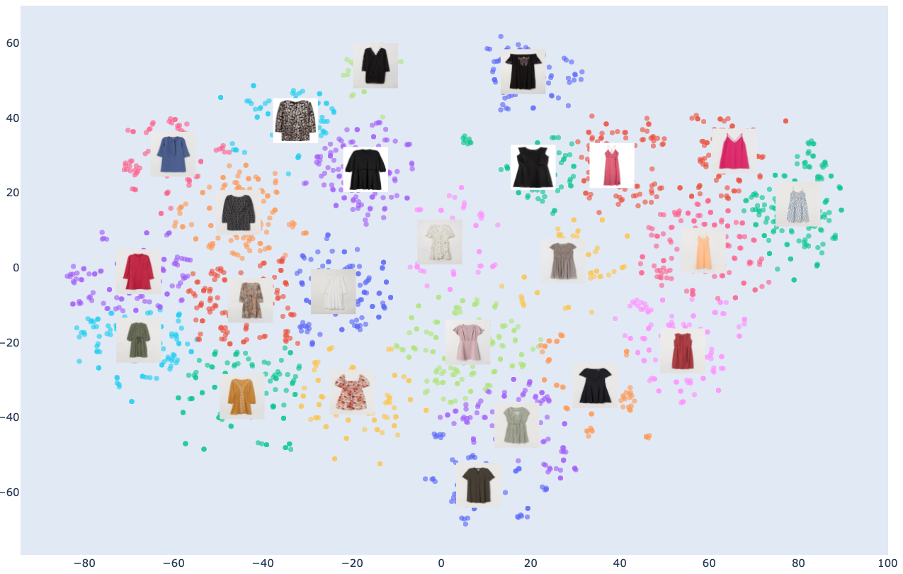
Figure 1: The Product Landscape

The x-axis and y-axis of this map are tSNE vectors that have compressed the combined embedding space from 1024 to 2 (to permit 2-dimensional visualization). Each dot represents a product, the colors represent that product have been assigned to different clusters (Kmeans clustering on the 2D tSNE vectors). The image shown in the middle of each cluster is of the most representative product in the cluster, i.e., the one with its tSNE 2D embedding closest to the cluster centroid. From the visualization, it is clear that the landscape of women’s dresses has a very distinct layout. On the right are sleeveless and shoulder based dresses, some are longer while some are shorter. Towards the bottom, you have dresses that look more like shirts, some with a puffed-out sleeve. Towards the right, you have longer and full-sleeved dresses. Some clusters identify the use of belts, while others are lace-oriented. There is an entire cluster for off-shoulders. Some clusters identify flower patterns, while others are more neutral. Below are some clusters with common phrases used in their descriptions (n-grams) and common product images.

While clusters should be spread apart, the products within a cluster should be similar to each other, displaying lesser variation. This fact is easily confirmed by looking at products within a few clusters. I also show a word cloud of n-grams in the text description of products in that cluster, giving us more information about the type of product there is.

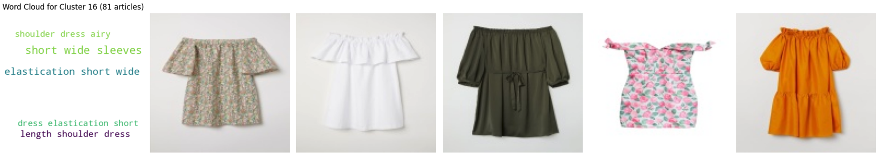
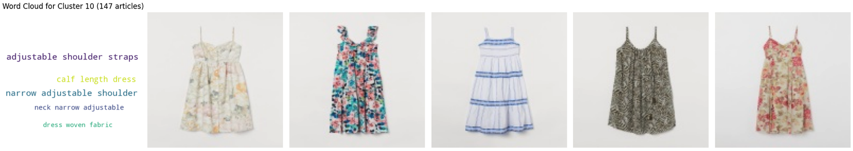
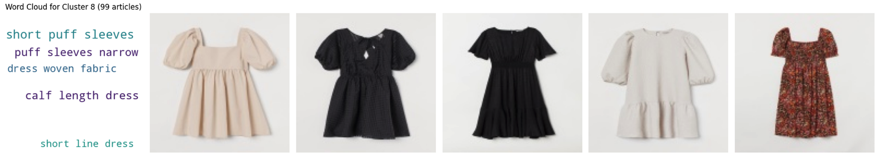
Figure 2: Distinct Clusters of Products

It should be noted that I have not manually categorized these products—the embeddings were rich and representative enough that it became easy to cluster them into neat categories. Of course, there may be some miscategorizations, but by and large, it is clear that the embeddings distinguish products into vector space in an intuitive way. This gives us confidence that we can use these embeddings in formal models.

6 Baseline Models

The variables used in our equations are defined as follows: $y_{i}$ represents the product purchased in consumer session $i$, $p_{j}$ is the price of product $j$, $X_{j}$ refers to the text and image embeddings of product $j$, and $D_{i}$ includes the demographics and temporal variables of consumer session $i$. There are $J$ products to choose from and $N$ consumer sessions that conclude with a sale, and utilities are given by,

$$u_{ij}=h(p_{j},D_{i},X_{j},\epsilon_{ij})$$

The choice made by each consumer is modeled as the product that maximizes their utility, expressed as,

$$y_{i}=\underset{j\in\{1,2,\ldots,J\}}{\text{argmax}}\ h(p_{j},D_{i},X_{j},\epsilon_{ij})$$

This leads to a probabilistic representation of consumer choices:

$$\mathbb{P}(y_{i}=j)=\int_{\epsilon_{ij}}h(p_{j},D_{i},X_{j},\epsilon_{ij})f(\epsilon_{ij})d\epsilon_{ij}$$

The utility function is assumed to be partially linear and separable:

$$h(p_{j},D_{i},X_{j})=h_{1}(p_{j},D_{i};\theta_{1})+h_{2}(X_{j},D_{i};\theta_{2})+\epsilon_{ij}$$

The model relies on independent and identical draws: $\{y_{i},p_{j},X_{j},D_{i}\}^{N}_{i=1}$. Key assumptions include no habit formation, adjustment costs, interference, and no unobserved heterogeneity. For unobservables, there is no unobserved $\xi_{j}$ term, meaning no unobserved confounders, and $\epsilon_{ij}$ is EV(1) and IID.

Given that $\epsilon_{ij}$ is EV(1) and IID across $j$ and $i$, we derive the following probability:

$$\mathbb{P}(y_{i}=j)=\frac{e^{h_{1}(p_{j},D_{i};\theta_{1})+h_{2}(X_{j},D_{i};\theta_{2})}}{\sum_{k}e^{h_{1}(p_{k},D_{i};\theta_{1})+h_{2}(X_{k},D_{i};\theta_{2})}}$$

This leads to the likelihood:

$$l(\theta)=\sum_{i}\sum_{j}1(y_{i}=j)\log\left(\frac{e^{h_{1}(p_{j},D_{i};\theta_{1})+h_{2}(X_{j},D_{i};\theta_{2})}}{\sum_{k}e^{h_{1}(p_{k},D_{i};\theta_{1})+h_{2}(X_{k},D_{i};\theta_{2})}}\right)$$

Estimation methods include $l^{\prime}(\theta)$ via backpropagation and hill climbing techniques, with standard errors calculated using Hessians and influence functions.

6.1 Homogenous $\alpha$

I estimate models from simple to complex, starting with the Conditional Logit (CL):

$$u_{ij}=\alpha p_{j}+\beta^{\prime}X_{j}+\epsilon_{ij}$$

and moving to more complex forms like the Partially Linear Logit with Heterogeneity (PLLH):

$$u_{ij}=\alpha p_{j}+g(X_{j},D_{i})+\epsilon_{ij}$$

$$u_{ij}=\alpha(D_{i})p_{j}+g(X_{j},D_{i})+\epsilon_{ij}$$

and the Nonlinear Logit (NLL):

$$u_{ij}=g(p_{j},X_{j},D_{i})+\epsilon_{ij}$$

The analysis of consumer choice models reveals significant insights into the preferences and decision-making processes of consumers. Our first set of results explores the impact of price logarithms and product features on consumer choices, employing different logit model specifications. The estimated coefficients for each model are presented in the table below. Standard errors are obtained using the methodology in Farell et al., (2021) (see Appendix 10.2 to 10.6).

Model	$\alpha$	Std Err	p-value
$u_{ij}=\alpha\log p_{j}+\beta^{\prime}X_{j}+\epsilon_{ij}$	-0.40	0.02	0.00
$u_{ij}=\alpha\log p_{j}+g(X_{j})+\epsilon_{ij}$	-0.26	0.02	0.00
$u_{ij}=\alpha\log p_{j}+g(X_{j},D_{i})+\epsilon_{ij}$	-0.37	0.02	0.00

Table 4: Homogenous Logit Results

The results from the constant-price sensitivity logit models show that using neural nets to estimate $g$ does allow covariates to steal some explanatory power from prices. This is as expected – ignoring the nonlinearity in how $X$ enters the utility function would lead us to overestimate $\alpha$. However, once we control for demographics, we see that consumers are more price-sensitive. This implies that not controlling for demographics leads to omitted variable bias in price.

6.2 Heterogeneous $\alpha$

Continuing our analysis, the model specifications were expanded to include demographics in $\alpha$. We start with a linear specification for $\alpha$,

$$\alpha(D_{i})=\alpha^{\prime}D_{i}$$

The coefficients from this expanded model are displayed in the subsequent table (without standard errors at the moment). Notably, customers who are receptive to active communications, those who are members of clubs, and older customers tend to exhibit higher price sensitivity. Conversely, customers who frequently listen to the news show a lower sensitivity to price variations.

Normalized Variable	Coefficient
Intercept	-0.4249
Active_1.0	-0.1551
FN_1.0	0.3864
Age	-0.0428
Club_Active	-0.1427
Club_Left	-0.1374
Club_Pre	0.0976
News_Freq_Monthly	0.0928
News_Freq_None	0.2663
News_Freq_Regularly	0.0343

Table 5: Extended Model Coefficients

At this stage, I have omitted postal code dummies from demographics to simplify the analysis, but they can be introduced later on to add to consumer heterogeneity, particularly across locations. Lastly, I allowed $\alpha$ to be specified as a full deep ReLU network. The corresponding utility function is,

$$u_{ij}=\alpha(d_{i})\log p_{j}+g(x_{j},d_{i})+\epsilon_{ij}$$

The results show a multi-modal distribution of $\alpha$, highlighting that different consumers have different price sensitivities. There also seems to be a “missing middle", indicating that working with avg. estimates might be misleading. Broadly, there seem to be two types of consumers, roughly equal in number - one with high sensitivity and one with lower.

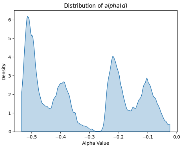
Figure 3: Distribution of $\alpha$ values

In our analysis using structural models, several key insights have been gathered regarding consumer behavior and price sensitivity. First, incorporating controls for images and text in the models increases observed price sensitivity. Moreover, when customer heterogeneity is accounted for, this sensitivity to price changes is further heightened. Furthermore, price sensitivities vary significantly among different customer segments. Specifically, these sensitivities range from -0.5 to -0.1. At the moment, I have not completed an analysis of the $g$ function, but that would help us get interesting counterfactuals involving diverse consumers and their aesthetic preferences.

7 Model Extensions

While the preceding models sought to capture heterogeneous product aesthetics and price sensitivities, there are still some important considerations. Extensions to the model allow us to cater to factors that could bias the results. The simplest enhancement features a broader set of demographics - computed from spending patterns in other categories. For instance, if an individual has spent on kids’ garments, we can deduce that they are in proximity to a child. Similarly, the total volume of spending the person has made on H&M can be used to measure brand affinity. The second important extension is to allow preferences to change according to the season the shopping decision was made. Seasonal trends can be easily incorporated by adding seasonal dummies. Thirdly, despite having a large number of demographic attributes, we may still be missing something, so it might make sense to allow for unobserved heterogeneity. A simple way of doing so for consumers is by adding unknown types to the likelihood estimation, as proposed by Heckman and Singer (1984). This increases the computational complications but allows the data to differentiate between users who are behaving differently - despite having no data to separate them. The last important extension is about price endogeneity. This is addressed by using a control function approach as described by Petrin and Train (2010). We do this by modeling unobserved confounders with first-stage residuals obtained by a regression of price on covariates and instruments. Flexible, functional forms can be chosen to allow unobserved confounders to be nonlinear in exogenous variation in prices.

The variables in the model are defined as follows: $p_{jt}$ represents prices, $D_{i}$ covers extended demographic attributes, $M_{j}$ denotes the product image, $T_{j}$ refers to the text description, $S_{t}$ indicates seasonal dummies and $k$ identifies the unobserved type. We typically will set $k=2$, increasing its value and stopping when the likelihood ceases to increase. The first few extension (barring instruments) is described below. The utility function for the $j$-th product for the $i$-th customer of type $k$ in period $t$ is expressed as:

$$U_{ijtk}=\alpha_{k}(D_{i},S_{t})\log p_{jt}+g_{k}(M_{j},T_{j},D_{i},S_{t})+\epsilon_{ijtk},$$

Given this, the probability that consumer $i$ chooses product $j$ is calculated by:

$$\mathbb{P}(y_{i}=j)=\sum_{k}\pi_{k}\frac{e^{\alpha_{k}(D_{i},S_{t})\log p_{jt}+g_{k}(M_{j},T_{j},D_{i},S_{t})}}{\sum_{j^{\prime}}e^{\alpha_{k}(D_{i},S_{t})\log p_{j^{\prime}t}+g_{k}(M_{j^{\prime}},T_{j^{\prime}},D_{i},S_{t})}}.$$

7.1 Price Endogeneity

The final set of extensions to account for price endogeneity is given as follows. Addressing price endogeneity involves using instruments $Z_{j}$ to model:

$$U_{ij}=\alpha(D_{i})\log p_{j}+g(M_{j},T_{j},D_{i})+\xi_{j}+\epsilon_{ij},$$

where $\xi_{j}$ is the omitted variable. The price equation is:

$$\log p_{j}=q(M_{j},T_{j},Z_{j})+v_{j}.$$

Residuals from this equation model the omitted variable:

$$\xi_{j}=\gamma(v_{j}).$$

With the estimated residuals $\hat{v_{j}}$, the probability function reshapes to:

$$\mathbb{P}(y_{i}=j)=\frac{e^{\alpha(D_{i})\log p_{j}+g(M_{j},T_{j},D_{i})+\gamma(\hat{v_{j}})}}{\sum_{j^{\prime}}e^{\alpha(D_{i})\log p_{j^{\prime}}+g(M_{j^{\prime}},T_{j^{\prime}},D_{i})+\gamma(\hat{v_{j^{\prime}}})}}.$$

8 Conclusion and Next Steps

In this paper, we find a few interesting insights. Firstly, in some markets, the visual aesthetic matters a lot. It is possible to capture these visual elements by using pre-trained embedding models on product images and text. These embeddings can explain up to half the variation in sales and two-thirds the variation in prices. They can also intuitively partition the product space and help us discover products close to each other. It is possible to also use these embeddings in economic models of brand choice or consumer demand. Estimation results from logit-based models show that incorporating consumer heterogeneity matters - the price sensitivity of consumers varies from -0.5 to -0.1. That is, for a 50% reduction in the price of a product, we foresee some sections of consumers increase purchases by only 5%, but other sections increase purchases by 25%. That is not a small amount of variation and it may be useful for retailers to be able to differentiate such consumers.

The road ahead for this paper is to control for seasonal and temporal variation in shopping trends and tackle econometric issues of unobserved heterogeneity and price endogeneity. There are also some important robustness checks required—sample splitting to eliminate regularization bias and out-of-time validation by observing how well this model predicts trends in the future. Once we have our model, we can use it to test counterfactuals. These include studying optimal discounting policies, new aesthetic design policies, and their welfare impact on consumers.

9 References

Jens Ludwig and Sendhil Mullainathan. Machine learning as a tool for hypothesis generation. NBER Working Papers, March 2023. Available at https://ideas.repec.org//p/nbr/nberwo/31017.html. Kenneth E. Train. Discrete choice methods with simulation. Cambridge University Press, June 2009. ISBN: 978-1-139-48037-6.

Steven T. Berry and Philip A. Haile. Foundations of demand estimation. In Handbook of Industrial Organization, Volume 4, pages 1-62. Elsevier, January 2021. doi:10.1016/bs.hesind.2021.11.001. Available at https://www.sciencedirect.com/science/article/pii/S1573448X21000017.

Victor Chernozhukov, Whitney Newey, Víctor M. Quintas-Martínez, and Vasilis Syrgkanis. RieszNet and ForestRiesz: Automatic debiased machine learning with neural nets and random forests. In Proceedings of the 39th International Conference on Machine Learning, pages 3901-3914. PMLR, June 2022. Available at https://proceedings.mlr.press/v162/chernozhukov22a.html.

Victor Chernozhukov, Denis Chetverikov, Mert Demirer, Esther Duflo, Christian Hansen, Whitney Newey, and James Robins. Double/debiased machine learning for treatment and causal parameters. arXiv:1608.00060 [econ, stat], December 2017. doi:10.48550/arXiv.1608.00060. Available at http://arxiv.org/abs/1608.00060.

Max H. Farrell, Tengyuan Liang, and Sanjog Misra. Deep learning for individual heterogeneity: An automatic inference framework. arXiv:2010.14694 [cs, econ, math, stat], July 2021. doi:10.48550/arXiv.2010.14694. Available at http://arxiv.org/abs/2010.14694.

Max H. Farrell, Tengyuan Liang, and Sanjog Misra. Deep neural networks for estimation and inference. Econometrica, 89(1):181-213, 2021. doi:10.3982/ECTA16901. Available at https://www.econometricsociety.org/doi/10.3982/ECTA16901.

Lorenzo Magnolfi, Jonathon McClure, and Alan T. Sorensen. Triplet embeddings for demand estimation. SSRN Scholarly Paper, October 2023. doi:10.2139/ssrn.4113399. Available at https://papers.ssrn.com/abstract=4113399.

Sukjin Han, Eric H. Schulman, Kristen Grauman, and Santhosh Ramakrishnan. Shapes as product differentiation: Neural network embedding in the analysis of markets for fonts. arXiv:2107.02739 [cs, econ], March 2024. doi:10.48550/arXiv.2107.02739. Available at http://arxiv.org/abs/2107.02739.

Giovanni Compiani, Ilya Morozov, and Stephan Seiler. Demand estimation with text and image data. SSRN Scholarly Paper, 2023. doi:10.2139/ssrn.4608817. Available at https://papers.ssrn.com/abstract=4608817.

Thomas W. Quan and Kevin R. Williams. Extracting characteristics from product images and their application to demand estimation.

Chengjun Zhang. Essays on consumer heterogeneity and personalized discounts in an online market. PhD Thesis, Georgetown University, February 2024.

10 Appendix

10.1 Deep ReLU Networks

Deep ReLU networks refer to deep neural networks that utilize the Rectified Linear Unit (ReLU) activation function within their hidden layers. Variables are defined as follows. Here, $\mathbf{x}$ represents the input vector to the network, consisting of features from the data. The weight matrix $\mathbf{W}^{(l)}$ and the bias vector $\mathbf{b}^{(l)}$ are components of the $l$-th layer of the network, responsible for performing linear transformations. The linear output $\mathbf{z}^{(l)}$ at each layer $l$ is calculated by $\mathbf{z}^{(l)}=\mathbf{W}^{(l)}\mathbf{a}^{(l-1)}+\mathbf{b}^{(l)}$, where $\mathbf{a}^{(l-1)}$ denotes the activation from the previous layer. Activation $\mathbf{a}^{(l)}$ at layer $l$ is defined through the ReLU function applied to $\mathbf{z}^{(l)}$, expressed as $\mathbf{a}^{(l)}=\text{ReLU}(\mathbf{z}^{(l)})$ where ReLU is formulated as $\text{ReLU}(x)=\max(0,x)$. Deep ReLU networks are typically composed of several layers where each layer consists of a linear transformation followed by the ReLU activation:

$$\mathbf{a}^{(l)}=\text{ReLU}(\mathbf{W}^{(l)}\mathbf{a}^{(l-1)}+\mathbf{b}^{(l)})$$

There are three main benefits of deep ReLU networks. Firstly, it reduces the chance of gradients becoming too small when the input becomes too small or too large (something common to the logistic function). As $x$ rises and is positive, the gradient remains capped at 1. This allows us to stack ReLUs and create very deep networks. Deep networks are better than wider networks due to parameter sharing; the network is forced to learn very abstract representations of the input, and this helps it generalize better. Secondly, when $x$ is below zero, the ReLU output is 0 (the neuron is shut off), and this introduces sparsity or a kind of automatic variable selection into the model. Thirdly, the ReLU operator is simple and computationally cheap.

The simplicity of ReLUs implies that the network effectively partitions the input space and applies separate linear functions to each region. Deep ReLU networks can potentially partition the input space so finely that it’s more interesting to ask how they can generalize at all and not just overfit every time. However, in practice, this does not happen, and ReLUs generalize well. Hanin and Rolnick (2019) show that untrained ReLU networks typically exhibit a number of linear regions growing linearly with the number of ReLU nodes. After training, this number grows polynomially in the number of ReLU nodes and exponentially with the depth.

10.2 Deep Neural Networks for Estimation and Inference

This section presents a simple model from Farell et al. (2021). I show how we can model parameters as deep ReLU neural networks and do hypothesis testing on them. I also show how we can use automatic differentiation and gradient descent to estimate the parameters and obtain inferences on any target statistic.

In our notation, $Y$ represents the outcome variable and falls within $\mathbb{R}^{d_{Y}}$. Similarly, $T$ denotes the treatment variable and resides in $\mathbb{R}^{d_{T}}$. The characteristics $X$ are elements of $\mathbb{R}^{d_{X}}$, and the parameters $\theta(X)$ belong to $\mathbb{R}^{d_{\theta}}$. The loss function $L$ maps from $\mathbb{R}^{d_{Y}+d_{T}+d_{\theta}}$ to $\mathbb{R}$, and the target value $\mu$ is in $\mathbb{R}^{d_{\mu}}$. The target function $H$ maps from $\mathbb{R}^{d_{X}+d_{\theta}}$ to $\mathbb{R}^{d_{\mu}}$, while the influence function $\Psi$ maps from $\mathbb{R}^{d_{Y}+d_{T}+d_{X}+d_{\theta}}$ to $\mathbb{R}^{n}$. The sample size is denoted by $n$.

Our methodology involves several key steps.

• Firstly, we define the parametric loss by finding $\theta_{0}(x)$ and $\theta_{1}(x)$ as the solutions to minimize the expected loss function $E[L(Y,T,\theta(X))]$, where $\theta$ is the parameter vector.

• Additionally, we compute the Expected Hessian denoted by $\Lambda(x)=E[L_{\theta\theta}|X,T]$, which provides insights into the curvature of the loss function.

• Next, we calculate the influence function $\Psi(y,t,x)$, which measures the change in the target $\mu$ (our metric of interest) for an infinitesimal change in the observation $(y,t,x)$. This function is derived from the difference between $H$ and the product of $H_{\theta}$ and $\Lambda(x)^{-1}L_{\theta}$.

• For estimation, we employ deep ReLU neural networks $\hat{\theta}_{0}(x)$ and $\hat{\theta}_{1}(x)$ to minimize the empirical loss. The parameters $\hat{H}_{\theta}$, $\hat{L}_{\theta}$, and $\hat{\Lambda}(x_{i})$ are obtained through automatic differentiation.

• Then, in the inference stage, we use the estimated parameters $\hat{\theta}_{0}(x_{i})$, $\hat{\theta}_{1}(x_{i})$, and $\hat{\Lambda}(x_{i})$ to compute $\hat{\Psi}(y_{i},t_{i},x_{i})$. Then, we calculate $\hat{\mu}$ as the average of $\hat{\Psi}(y_{i},t_{i},x_{i})$ over the sample size $n$.

• Lastly, we estimate the variance $\hat{\text{Avar}(\hat{\mu})}$ as the average squared deviation of $\hat{\Psi}(y_{i},t_{i},x_{i})$ from $\hat{\mu}$.

10.3 Real world example

Imagine we are analysing an A/B Test, we analyze how a new app design ($T$) affects user engagement, specifically the time spent on the app ($Y$). The model for this relationship is $Y_{i}=\theta_{0}(X_{i})+\theta_{1}(X_{i})T_{i}+V_{i}$. Here, $Y_{i}$ is the time spent by user $i$. The function $\theta_{0}(X_{i})$ represents the baseline engagement, and $\theta_{1}(X_{i})$ measures the impact of the new app design on user $i$. The term $V_{i}$ accounts for other unseen factors that affect engagement. Random assignment of the design ensures that $E[V_{i}|T_{i}]=0$ and $E[T_{i}|X_{i}]=E[T_{i}]$. We use the loss function $L=(Y-\theta_{0}(X_{i})-\theta_{1}(X_{i})T_{i})^{2}$ to compute the squared difference between observed and predicted times. Our primary interest is the Average Treatment Effect (ATE), which we represent as $H(X,\theta(X))=E[\theta_{1}(X_{i})]$. This shows the average expected change in engagement due to the new design across different user demographics. The main advantage of this approach is that $X$ can be very high dimensional, and we would be able to obtain heterogeneous treatment effects when parameters $\theta_{1}$ in a deep ReLU network.

10.4 Influence Functions

Given a set of independent and identically distributed (IID) data points $Z_{i}\sim F$, an influence function evaluates the impact of a specific data point $z$ on a particular statistic $\mu=T(F)$. To quantify this influence, we consider a contaminated distribution $F_{\epsilon}$, where $\epsilon$ is a small perturbation parameter, and $\delta_{z}$ is a cumulative distribution function (CDF) that equals 1 after $Z=z$ and 0 before. The Influence Function is formally defined as $\Psi_{F,\mu}(z)=\lim_{\epsilon\rightarrow 0}\frac{T(F_{\epsilon})-T(F)}{\epsilon}$.

Here are some examples to illustrate influence functions: - For the mean $\mu_{Z}=T(F)=\int zdF(z)$, the influence function is $\Psi(z)=z-\mu_{Z}$, representing the deviation of the data point from the mean. - For the variance $\sigma^{2}_{Z}=T(F)=\int(z-\mu_{Z})^{2}dF(z)$, the influence function is $\Psi(z)=(x-\mu_{Z})^{2}-\sigma^{2}_{Z}$, indicating how a change in the data point affects the variance. - For the $q$-quantile $\mu_{q}=T(F)=F^{-1}(q)$, the influence function depends on whether the data point is less than or greater than the quantile value $\mu_{q}$. It is given by:

$$\Psi(z)=\begin{cases}\frac{q-1}{f(\mu_{q})},&\text{if }x\leq\mu_{q}\\ \frac{q}{f(\mu_{q})},&\text{otherwise}\end{cases}$$

where $f(\mu_{q})$ is the probability density function evaluated at $\mu_{q}$.

Estimating Influence Functions can be approached in two ways:

Parametrically: This involves finding a closed-form expression for $\Psi(z)$ based on the distributional assumptions and then substituting sample estimates into the formula.

Nonparametrically: Here, the influence function is computed by reevaluating the statistic with one observation omitted (Jackknife method) and comparing it to the original estimate.

10.5 Example: Linear Model with Deep Parameters

The Data Generating Process (DGP) involves a binary treatment $T$ that is randomized, high-dimensional covariates $X$, and a continuous outcome $y$. The objective is to estimate $\theta(x)$ and perform inference on $\mu=E[\theta_{1}(x)]$, representing the average treatment effect.

$$y_{i} =\alpha_{i}+\beta_{i}T_{i}+u_{i},\quad u_{i}\sim N(0,1)$$

$$\alpha_{i} =\theta_{0}(x_{i}),\quad\beta_{i}=\theta_{1}(x_{i})$$

$$\theta_{0}(x_{i}) =0.2x_{1i}-0.3x_{2i}-0.5x_{3i}$$

$$\theta_{1}(x_{i}) =2-x_{2i}-0.25x_{1i}^{3}$$

Considering $T$ as binary, where $T^{2}=T$ and $E[T|X=x]=p(x)$ denotes the propensity score. If $T$ is randomized, then $p(x)=E[T]$.

$$L(y,t,\theta(x)) =0.5(y-\theta_{0}(x)-\theta_{1}(x)T)^{2}$$

$$L_{\theta} =\begin{bmatrix}L_{\theta_{0}}\\ L_{\theta_{1}}\end{bmatrix}=\begin{bmatrix}-(y-\theta_{0}(x)-\theta_{1}(x)T)\\ -T(y-\theta_{0}(x)-\theta_{1}(x)T)\end{bmatrix}$$

$$L_{\theta_{0}\theta_{1}} =T,\quad L_{\theta_{0}\theta_{0}}=1,\quad L_{\theta_{1}\theta_{1}}=T^{2}$$

$$\Lambda(x) =E[L_{\theta\theta}|X=x]=\begin{bmatrix}1&E[T|X=x]\\ E[T|X=x]&E[T^{2}|X=x]\end{bmatrix}=\begin{bmatrix}1&p(x)\\ p(x)&p(x)\end{bmatrix}$$

The target function $\mu$ is defined as $E[H(X,\theta(X);T=1)]=E[\theta_{1}(X)]$, where $H(X,\theta(X);T=1)=\theta_{1}(X)$. The gradient of the target function with respect to $\theta$ is denoted as $H_{\theta}$, given by:

$$H_{\theta}=\begin{bmatrix}H_{\theta_{0}}&H_{\theta_{1}}\end{bmatrix}=\begin{bmatrix}0&1\end{bmatrix}$$

The influence function $\Psi(y,t,x)$ can be derived as follows:

$$\Psi(y,t,x) =H-H_{\theta}\Lambda(x)^{-1}L_{\theta}$$

$$\Psi(y,t,x) =\theta_{1}(x)-\begin{bmatrix}0&1\end{bmatrix}\begin{bmatrix}1&p(x)\\ p(x)&p(x)\end{bmatrix}^{-1}\begin{bmatrix}-(y-\theta_{0}(x)-\theta_{1}(x)T)\\ -T(y-\theta_{0}(x)-\theta_{1}(x)T)\end{bmatrix}$$

$$\Psi(y,t,x) =\theta_{1}(x)+\frac{t(y-\theta_{0}(x)-\theta_{1}(x)t)}{p(x)}+\frac{(1-t)(y-\theta_{0}(x))}{1-p(x)}$$

Data consists of $\{y_{i},x_{i},t_{i}\}^{n}_{i=0}$. A neural network $\theta(x;\gamma)$ is employed, where $x\in\mathbb{R}^{5}$ serves as inputs, and there are two hidden layers with 20 neurons each, producing outputs $\theta_{0}(x)$ and $\theta_{1}(x)$. The empirical loss function $\hat{L}$ is defined as $\frac{1}{2}\frac{1}{n}\sum_{i}(y_{i}-\theta_{0}(x_{i})-\theta_{1}(x_{i})t_{i})^{2}$. Gradient descent is utilized for parameter optimization: $\gamma_{k+1}\leftarrow\gamma_{k}-\tau\frac{d\hat{L}}{d\gamma}$. The estimated parameters are denoted as $\hat{\theta}(x_{i})=\theta(x_{i};\gamma_{K})$.

In the estimation process, $\alpha_{i}$ and $\beta_{i}$ are defined as the estimated coefficients $\hat{\theta}_{0}(x_{i})$ and $\hat{\theta}_{1}(x_{i})$, respectively. The gradients $\hat{L}_{\theta}$ are computed as:

$$\hat{L}_{\theta}=\begin{bmatrix}\frac{\hat{L}}{d\alpha_{0}}&\frac{\hat{L}}{d\beta_{0}}\\ \frac{\hat{L}}{d\alpha_{1}}&\frac{\hat{L}}{d\beta_{1}}\\ \vdots&\vdots\\ \frac{\hat{L}}{d\alpha_{N}}&\frac{\hat{L}}{d\beta_{N}}\end{bmatrix}$$

The Hessian matrix $\hat{\Lambda}(x_{i})$ is expressed as:

$$\hat{\Lambda}(x_{i})=\begin{bmatrix}\frac{1}{n}\sum_{i}\frac{\hat{L}}{d\alpha_{0}^{2}}&\frac{\hat{L}}{d\beta_{0}}\\ \frac{\hat{L}}{d\alpha_{1}}&\frac{\hat{L}}{d\beta_{1}}\\ \vdots&\vdots\\ \frac{\hat{L}}{d\alpha_{N}}&\frac{\hat{L}}{d\beta_{N}}\end{bmatrix}$$

Here is how we do inference. Split the sample into 3 parts:

• Sample 1 $S_{1}$: Estimate $\hat{\theta}$

• Sample 2 $S_{2}$: Use $\hat{\theta}$, to estimate $\hat{\Lambda}(x)$

• Sample 3 $S_{3}$: Use $\hat{\theta},\hat{\Lambda}(x)$, to compute $\hat{\Psi}$

$$\hat{\Psi}(y_{i},t_{i},x_{i})=\hat{\theta}_{1}(x_{i})+\frac{t_{i}(y_{i}-\hat{\theta}_{0}(x_{i})-\hat{\theta}_{1}(x_{i})t_{i}}{\hat{p}(x_{i})}+\frac{(1-t_{i})(y_{i}-\hat{\theta}_{0}(x_{i})}{1-\hat{p}(x_{i})}$$

$$\hat{\mu}=(1/n_{S_{3}})\sum_{i}\hat{\Psi}(y_{i},t_{i},x_{i})$$

$$\hat{\text{Avar}}(\mu)=(1/n_{S_{3}})\sum_{i}(\hat{\Psi}(y_{i},t_{i},x_{i})-\hat{\theta}_{1}(x_{i}))^{2}$$

Sample splitting is unnecessary if $T$ is randomized or if $\Lambda(x)$ does not depend on $\theta$.

10.6 Example: Binary Logit with Deep Parameters

$T$ is a binary treatment that is randomized, $Y$ is binary outcome, $X$ are high dimensional covariates.

$$u_{i} =\alpha_{i}+\beta_{i}T_{i}+u_{i},\quad u_{i}\sim N(0,1)$$

$$p_{i} =P[y_{i}=1]=G(T_{i})=\frac{1}{1+e^{-u_{i}}}$$

$$y_{i} =1(p_{i}>0.5)$$

$$\alpha_{i} =\theta_{0}(x_{i}),\beta_{i}=\theta_{1}(x_{i})$$

$$\theta_{0}(x_{i}) =0.2x_{1i}-0.3x_{2i}-0.5x_{3i}$$

$$\theta_{1}(x_{i}) =2-x_{2i}-0.25x_{1i}^{3}$$

We want to estimate and do inference on $\mu=E[\frac{dP[y_{i}=1]}{dT}]$ (Avg. Marginal Effect).

Loss and derivatives:

$$p=G(\alpha+\beta t)=\frac{1}{1+e^{\alpha+\beta t}}$$

$$L=-y_{i}\log p-(1-y)\log(1-p)$$

Since $1-G(z)=G(-z)$ and $G^{\prime}(z)=G(z)(1-G(z))$, we get,

• $\frac{dL}{d\alpha}=-y(1-p)+(1-y)p$

• $\frac{dL}{d\beta}=-yt(1-p)+(1-y)tp$

• $\frac{dL}{d\alpha^{2}}=p(1-p)$

• $\frac{dL}{d\beta^{2}}=t^{2}p(1-p)$

• $\frac{dL}{d\alpha\beta}=tp(1-p)$

Gradients and Hessian:

$$L_{\theta}=\begin{bmatrix}-y(1-p)+(1-y)p\\ -yt(1-p)+(1-y)tp\\ \end{bmatrix}$$

$$\Lambda(x)=E[G(\theta(x)^{\prime}T)(1-G(\theta(x)^{\prime}T))TT^{\prime}|X=x]$$

$$=E[p(1-p)\begin{bmatrix}1&t\\ t&t^{2}\\ \end{bmatrix}|X=x]$$

Target Gradients:

$$\mu=E[\frac{dG(\alpha+\beta t)}{dT}|T=t^{*}=E[T]]$$

$$=E[p(1-p)\beta]$$

$$H=p(1-p)\beta$$

$$H_{\alpha}=G(\alpha+\beta t)(1-G(\alpha+\beta t))\beta$$

The rest of the setup proceeds as with the Deep Linear Regression model.

10.7 Convolutional Neural Networks (CNNs)

Convolutional Neural Networks (CNNs) are tailored for processing grid-like data, such as images, using convolution operations rather than standard matrix multiplications. This approach effectively captures spatial hierarchies. CNN architectures consist of layers that progressively transform the input image to highlight specific features. Key components include convolutional layers, pooling layers, and fully connected layers.

Convolutional layers utilize learnable filters that operate over local input regions to build complex patterns from simpler elements. The convolution is mathematically represented as:

$$s(i,j)=(I*K)(i,j)=\sum_{m}\sum_{n}I(m,n)K(i-m,j-n),$$

where $I$ is the input image, $K$ is the filter, $s(i,j)$ is the output feature map, and $*$ indicates the convolution process. This operation isolates local feature information, initially ignoring global structure.

Pooling layers follow, reducing the spatial dimensions of the feature maps, thereby decreasing parameter count and computational load and enhancing feature invariance to scale and orientation shifts. Fully connected layers at the architecture’s end integrate the extracted data to produce final predictions, with each neuron connected to all activations from the previous layer, synthesizing the global information.

CNNs are highly effective for tasks like image recognition, classification, and segmentation due to their ability to recognize and interpret visual patterns directly from raw images with minimal preprocessing. The architecture’s design allows it to adapt to variations and distortions in data, progressively extracting more complex features at higher layers and forming a comprehensive visual understanding.

10.8 Attention Mechanism

The attention mechanism refines neural network capabilities by selectively concentrating on pertinent parts of the input data, used extensively in processing both textual and visual information. This mechanism optimizes the interpretation and management of sequential and spatial data. Each input component, whether a sequence or spatial element, is associated with features that contribute to computing attention weights. These weights determine the relevance of each element within a specific task context.

Variables are defined as follows: $\mathbf{x}_{i}$ represents the input features for the $i$-th element. $\mathbf{h}_{i}$ is the transformation-derived embedded representation of $\mathbf{x}_{i}$, through a neural network layer. $\mathbf{V}$ is a trainable parameter vector essential for calculating attention scores, while $\lambda$ modulates the attention distribution’s focus. The attention weights $\alpha_{i}$ are given by:

$$\alpha_{i}=\frac{\exp(\mathbf{h}_{i}^{T}\mathbf{V}/\lambda)}{\sum_{j}\exp(\mathbf{h}_{j}^{T}\mathbf{V}/\lambda)}$$

The weighted sum of these embeddings, known as the context vector $\mathbf{c}$, is:

$$\mathbf{c}=\sum_{i}\alpha_{i}\mathbf{h}_{i}$$

In textual applications, $\mathbf{h}_{i}$ usually denotes the embedded representation of the $i$-th word or token, assembling a context vector $\mathbf{c}$ that encapsulates the text’s essential segments as identified by $\alpha_{i}$. This process is pivotal in enhancing performance in tasks like summarization, translation, and sentiment analysis.

For image tasks, $\mathbf{h}_{i}$ relates to features from specific image patches or regions. Here, the attention mechanism dynamically prioritizes informative image areas for tasks such as object detection and captioning. The resulting context vector $\mathbf{c}$ aggregates significant visual features, steered by the spatial attention weights $\alpha_{i}$.

10.9 Transformers

Transformers are adept at managing long-range dependencies in natural language and image processing. Distinct from traditional sequential data processing models, transformers utilize parallel processing through an encoder and decoder structure composed of multiple identical layers.

The process begins by converting input data into dense vector representations or input embeddings $\mathbf{x}_{i}$. These embeddings are linearly transformed to generate three critical components for the self-attention mechanism: Query ($\mathbf{Q}$), Key ($\mathbf{K}$), and Value ($\mathbf{V}$), each through distinct trainable weight matrices ($\mathbf{W}^{Q}$, $\mathbf{W}^{K}$, and $\mathbf{W}^{V}$):

$$\mathbf{Q}=\mathbf{W}^{Q}\mathbf{x},\quad\mathbf{K}=\mathbf{W}^{K}\mathbf{x},\quad\mathbf{V}=\mathbf{W}^{V}\mathbf{x}$$

Here, $\mathbf{Q}$ matrices query which items to focus on, $\mathbf{K}$ matrices determine the attention each query should get, and $\mathbf{V}$ matrices carry the actual content to be compiled into the output based on these interactions. The self-attention mechanism computes attention scores to dictate how input elements influence one another:

$$\text{Scores}=\frac{\mathbf{Q}\mathbf{K}^{T}}{\sqrt{d_{k}}}$$

where $d_{k}$ is the Key vectors’ dimensionality. These scores undergo softmax normalization to ensure they sum to one, forming:

$$\mathbf{A}=\text{softmax}(\text{Scores})$$

The self-attention layer’s output, $\mathbf{h}$, is then calculated by multiplying $\mathbf{A}$ with $\mathbf{V}$, serving as input for subsequent layers or further processing within the current layer:

$$\mathbf{h}=\mathbf{A}\mathbf{V}$$

Each encoder layer includes a multi-head self-attention mechanism, enabling simultaneous exploration of various attention perspectives coupled with a position-wise fully connected feed-forward network. The decoder replicates the encoder’s structure but incorporates an additional layer of multi-head attention focusing on the encoder’s output. Positional encodings are added to input embeddings to convey position information within the sequence, compensating for the self-attention mechanism’s lack of sequential order.

10.10 Contrastive Language–Image Pre-training (CLIP)

CLIP integrates visual and textual data, aligning image $M_{j}$ and text $T_{j}$ embeddings. The image encoder transforms $M_{j}$ into a visual vector $\mathbf{v}_{j}$, while the text encoder processes $T_{j}$ into a textual vector $\mathbf{t}_{j}$. The objective is precise alignment: the textual description should accurately reflect the image content, facilitated through a contrastive loss mechanism.

Define $\mathbf{v}_{j}$ as the visual embedding and $\mathbf{t}_{j}$ the textual embedding. Consider another image-text pair, denoted $\mathbf{v}_{k}$ and $\mathbf{t}_{k}$. The loss function increases with similarity $S(\mathbf{v}_{j},\mathbf{t}_{j})$ for correct pairs and decreases $S(\mathbf{v}_{j},\mathbf{t}_{k})$ for incorrect pairs. The loss for image $M_{j}$ against a batch of texts is given by:

$$L_{j}=-\log\frac{\exp(\text{sim}(\mathbf{v}_{j},\mathbf{t}_{j})/\tau)}{\sum_{k=1}^{N}\exp(\text{sim}(\mathbf{v}_{j},\mathbf{t}_{k})/\tau)}$$

The similarity function $\text{sim}(\mathbf{v},\mathbf{t})$ typically involves dot product or cosine similarity, with temperature $\tau$ adjusting the sharpness of distribution. The numerator emphasizes similarity for correct matches, while the denominator diffuses it across all pairs. By applying negative log-likelihood, the model refines the likelihood of correct image-text pairings against the batch. For this study, we employed the Fashion CLIP, trained specifically on fashion-related image-text pairs.

10.11 Autoencoders

Autoencoders are a neural network architecture focused on dimensionality reduction and feature learning. They operate by encoding high-dimensional input data into a compressed latent space representation and then reconstructing the original input from this representation with minimal fidelity loss. This is akin to dimensionality reduction methods like t-SNE but executed through a learnable neural network.

Variables in this framework include: $\mathbf{x}$, representing the original high-dimensional input data (e.g., images, text embeddings); $\mathbf{f}$, the encoder function which transforms the input data to a lower-dimensional latent space; and $\mathbf{r}$, the decoder function that maps the latent space back to the high-dimensional space to reconstruct the input. The effectiveness of an autoencoder is quantified using a loss function, often the Mean Squared Error (MSE), which measures the discrepancy between the original input and its reconstruction:

$$L(\mathbf{x},\mathbf{f},\mathbf{r})=\|\mathbf{x}-\mathbf{r}(\mathbf{f}(\mathbf{x}))\|^{2}$$

The latent space, denoted as $\mathbf{z}=\mathbf{f}(\mathbf{x})$, is crucial, capturing essential features of the input data in a compressed format. Beyond simple dimensionality reduction, autoencoders are employed in developing generative models of data.

10.12 t-Distributed Stochastic Neighbor Embedding (t-SNE)

t-SNE is a sophisticated technique for dimensionality reduction. It operates by converting data point similarities into joint probabilities and then minimizing the Kullback-Leibler divergence between these probabilities in both the high-dimensional and reduced low-dimensional spaces. High-dimensional probabilities, $p_{ij}$, are derived using a Gaussian distribution centered on each data point $x_{i}$:

$$p_{ij}=\frac{\exp(-\|x_{i}-x_{j}\|^{2}/2\sigma_{i}^{2})}{\sum_{k\neq i}\exp(-\|x_{i}-x_{k}\|^{2}/2\sigma_{i}^{2})}$$

where $\sigma_{i}$ is the variance, adjusted for each data point to capture the local data density accurately.

In the resultant low-dimensional space, probabilities $q_{ij}$ utilize a t-distribution:

$$q_{ij}=\frac{(1+\|y_{i}-y_{j}\|^{2})^{-1}}{\sum_{k\neq l}(1+\|y_{k}-y_{l}\|^{2})^{-1}}$$

Here, $y_{i}$ and $y_{j}$ represent the low-dimensional embeddings of $x_{i}$ and $x_{j}$, respectively. This method surpasses PCA in its capacity to capture more intricate structures by employing a non-linear approach, maintaining local relationships, and elucidating data clusters across various scales, often at the expense of global data structure representation. t-SNE’s primary strength lies in its ability to generate intuitive, visually appealing mappings.

10.13 K-Means Clustering

K-means clustering is an algorithm used for segmenting a dataset into $k$ predefined clusters. The variables are defined as follows: $n$ is the total number of observations in the dataset, $K$ represents the number of features each observation possesses, and $k$ indicates the number of clusters. Each observation $x$ is a vector in $d$-dimensional space, where $d$ signifies the number of features or attributes. $S_{i}$ denotes the set of all observations assigned to the $i$-th cluster, while $\mu_{i}$ is the centroid or the mean point of cluster $i$, calculated as the average of all observations $x$ in $S_{i}$. The squared Euclidean distance between an observation $x$ and the centroid $\mu_{i}$ is given by $\|x-\mu_{i}\|^{2}$. The objective function, $J$, known as the within-cluster sum of squares (WCSS), is defined as:

$$J=\sum_{i=1}^{k}\sum_{x\in S_{i}}\|x-\mu_{i}\|^{2}$$

The goal is to minimize $J$, enhancing cluster compactness and separation, ensuring observations within a cluster are closely grouped while each cluster is distinct from others.

The K-Means algorithm operates through several steps:

• Initialization: Select $k$ random points as initial centroids.

• Assignment: Assign each observation to the nearest centroid using Euclidean distance.

• Update: Recompute centroids as the mean of assigned observations.

• Iteration: Repeat the assignment and update until centroids stabilize or a set iteration limit is reached.

This algorithm’s effectiveness is contingent on the initial centroid selection and the number of clusters $k$. Suboptimal initial centroids can lead to poor clustering quality. K-Means++ addresses this by enhancing initial centroid distribution, potentially improving clustering outcomes. Selecting an optimal $k$ is critical; the elbow method is commonly used, plotting the sum of squared distances from points to their cluster centers against different $k$ values to identify the elbow point, beyond which increasing $k$ yields diminishing returns.

10.14 Random Forests and Boosting Machines

Tree-based methods apply to both classification and regression, using feature space partitions to minimize variance. For regression, a decision tree optimizes splits in dataset $\mathbf{D}=\{(\mathbf{x}_{i},y_{i})\}_{i=1}^{N}$ based on feature vectors $\mathbf{x}_{i}$ and targets $y_{i}$, using mean squared error (MSE):

$$\text{MSE}=\frac{1}{N}\sum_{i=1}^{N}(y_{i}-\overline{y})^{2},\quad\overline{y}=\frac{1}{N}\sum_{i=1}^{N}y_{i}$$

Splits are made by selecting feature $x_{j}$ and threshold $s$:

$$\text{Split}(\mathbf{D},j,s)=\{\mathbf{D}_{l},\mathbf{D}_{r}\}\quad\text{where}\quad\mathbf{D}_{l}=\{\mathbf{x}_{i}\in\mathbf{D}\mid x_{ij}\leq s\},\mathbf{D}_{r}=\{\mathbf{x}_{i}\in\mathbf{D}\mid x_{ij}>s\}$$

Here, the objective is to minimize combined MSE of $\mathbf{D}_{l}$ and $\mathbf{D}_{r}$. Splits are made recursively, in a tree like manner.

Random Forests: Utilize ensemble of trees from bootstrapped data subsets, each tree uses random feature subset at each split. The final output is the average of all trees:

$$\hat{y}=\frac{1}{T}\sum_{t=1}^{T}f_{t}(\mathbf{x}),\quad f_{t}\text{ is the }t\text{-th tree}$$

Gradient Boosting Machines (GBMs): Build trees sequentially to fit current residuals, updating via:

$$f_{t+1}(\mathbf{x})=f_{t}(\mathbf{x})+\eta\cdot h_{t}(\mathbf{x}),\quad h_{t}=\arg\min_{h}\sum_{i=1}^{N}(y_{i}-f_{t}(\mathbf{x}_{i})-h(\mathbf{x}_{i}))^{2}$$

Here, $h_{t}(\mathbf{x})$ adjusts the previous tree’s errors, with $\eta$ controlling update size. GBMs refine models by optimizing $\mathcal{L}$, often squared error loss. Random forests improve generalizability by averaging independent models, while GBMs enhance accuracy by sequentially reducing errors, risking overfitting if not calibrated.

10.15 OLS and Regularization

This section examines OLS, Lasso, and Ridge regression. Given an IID dataset $\mathbf{D}=\{(\mathbf{x}_{i},y_{i})\}_{i=1}^{N}$, with $\mathbf{x}_{i}$ as the feature vector of the $i$-th instance and $y_{i}$ the target, the OLS estimator $\boldsymbol{\beta}$ is computed via:

$$\boldsymbol{\beta}=(\mathbf{X}^{T}\mathbf{X})^{-1}\mathbf{X}^{T}\mathbf{y}$$

Here, $\mathbf{X}$ denotes the input feature matrix and $\mathbf{y}$ the target vector. Ridge regression modifies OLS by integrating a penalty $\lambda$ on the squared magnitude of coefficients, enhancing stability and handling multicollinearity or underdetermined datasets:

$$\boldsymbol{\beta}^{ridge}=(\mathbf{X}^{T}\mathbf{X}+\lambda\mathbf{I})^{-1}\mathbf{X}^{T}\mathbf{y}$$

Lasso applies a penalty on the absolute values of the coefficients, promoting sparsity and enabling feature selection, useful in high-dimensional settings:

$$\boldsymbol{\beta}^{lasso}=\arg\min_{\boldsymbol{\beta}}\left\{\frac{1}{2N}\|\mathbf{y}-\mathbf{X}\boldsymbol{\beta}\|_{2}^{2}+\lambda\|\boldsymbol{\beta}\|_{1}\right\}$$

Ridge and Lasso are penalized regression models adjusting the OLS objective to include regularization terms. Ridge is preferred for reducing coefficient magnitude in multicollinear scenarios, while Lasso is favored for feature reduction, offering inherent feature selection.

10.16 Bias-Variance Tradeoff in High-Dimensional Regression

In high-dimensional regression, where feature count $p$ may approach or exceed the number of observations $N$, understanding the bias-variance tradeoff is critical for model performance. Considering a dataset $\mathbf{D}=\{(\mathbf{x}_{i},y_{i})\}_{i=1}^{N}$ with $\mathbf{x}_{i}\in\mathbb{R}^{p}$ as the feature vector and $y_{i}\in\mathbb{R}$ as the target, the target-predictor relationship is modeled as $y_{i}=f(\mathbf{x}_{i})+\epsilon_{i}$, with $\epsilon_{i}$ denoting irreducible error, normally distributed with zero mean and variance $\sigma^{2}$.

The regression goal is typically to minimize the expected prediction error, quantified by mean squared error (MSE), which decomposes into three components:

$$\text{MSE}=\mathbb{E}[(y-\hat{f}(\mathbf{x}))^{2}]=\text{Bias}^{2}(\hat{f}(\mathbf{x}))+\text{Variance}(\hat{f}(\mathbf{x}))+\sigma^{2}$$

Bias is the difference between the model’s expected prediction and the true value:

$$\text{Bias}(\hat{f}(\mathbf{x}))=\mathbb{E}[\hat{f}(\mathbf{x})]-f(\mathbf{x})$$

Variance measures the spread of model predictions around their expected value:

$$\text{Variance}(\hat{f}(\mathbf{x}))=\mathbb{E}[(\hat{f}(\mathbf{x})-\mathbb{E}[\hat{f}(\mathbf{x})])^{2}]$$

In high-dimensional contexts, Ordinary Least Squares (OLS) often yield a low-bias but high-variance estimator, especially as $p/N$ rises. This can lead to overfitting, where the model learns noise rather than the underlying pattern, adversely affecting its generalization to new data.

Regularization techniques like Ridge and Lasso adjust OLS by introducing penalties on the coefficients to mitigate overfitting and effectively manage the bias-variance tradeoff. Regularization is also essential for other models like neural networks, Gradient Boosting Machines (GBMs), and Random Forests, where it helps control model complexity and improves generalizability across various data scenarios.

11 Figures

Figure 11: No. of Distinct Articles Selling Every Day Over Time

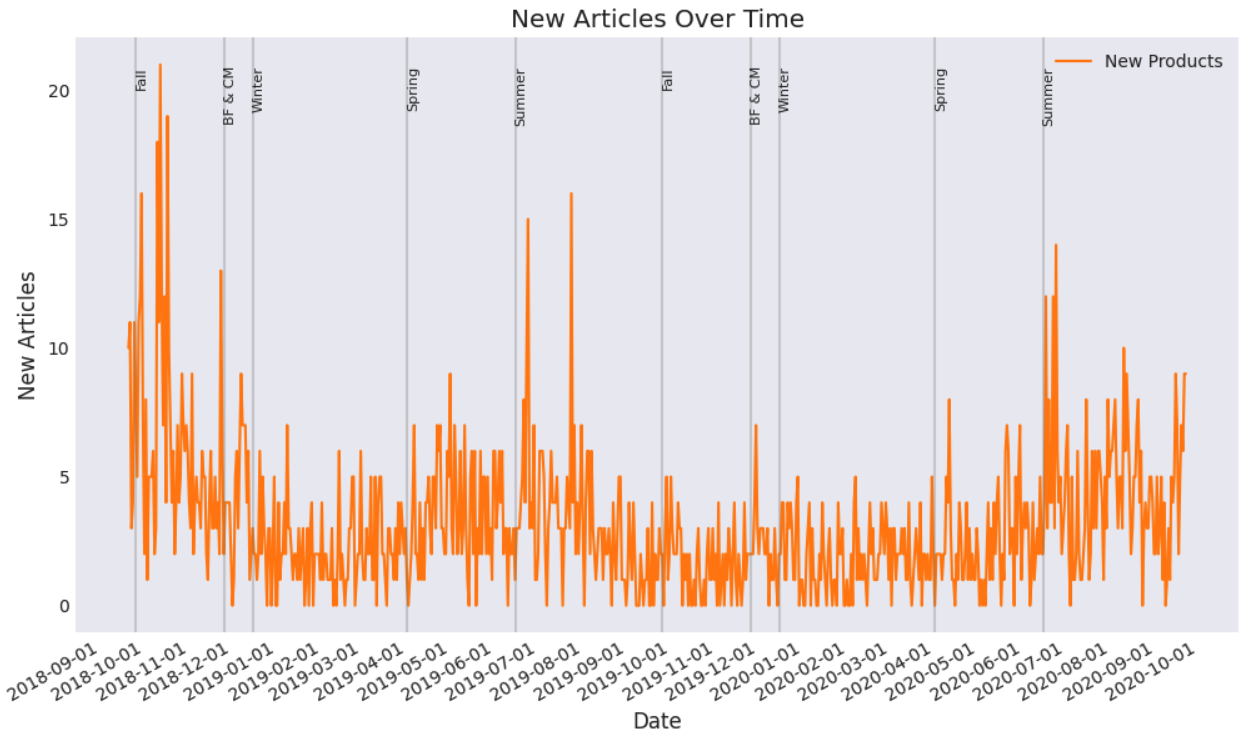
Figure 12: No. of Articles Observed For The First Time Over Time

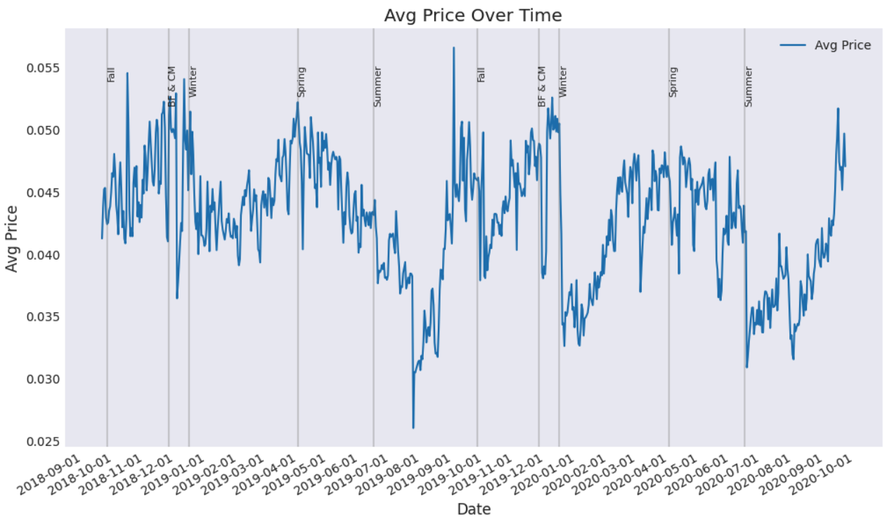
Figure 13: Avg Prices over Time

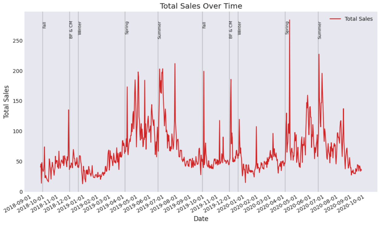
Figure 14: Total Sales Over Time

Figure 15: Total Spend Volumes over Time