Convexification for a Coefficient Inverse Problem for a System of Two Coupled Nonlinear Parabolic Equations

Abstract

A system of two coupled nonlinear parabolic partial differential equations with two opposite directions of time is considered. In fact, this is the so-called “Mean Field Games System” (MFGS), which is derived in the mean field games (MFG) theory. This theory has numerous applications in social sciences. The topic of Coefficient Inverse Problems (CIPs) in the MFG theory is in its infant age, both in theory and computations. A numerical method for this CIP is developed. Convergence analysis ensures the global convergence of this method. Numerical experiments are presented.

Key Words: a nonlinear parabolic system, Carleman estimates, convexification numerical method, global convergence analysis, numerical experiments

2020 MSC codes: 35R30, 91A16

1 Introduction

A system of two nonlinear parabolic partial differential equations with two opposite directions of time is considered. This is the so-called “Mean Field Games System” (MFGS), which is derived in the mean field games (MFG) theory [1]. This theory is about the mass behavior of infinitely many agents, who are assumed to be rational. Due to a rapidly growing number of applications of the MFG theory in social sciences, it makes sense to study a variety of mathematical questions for the MFGS. We are interested in a Coefficient Inverse Problem (CIP) for this system. Our unknown coefficient $k\left(x\right)$ characterizes a reaction of a controlled agent to an action applied at the point $x\in\Omega,$ where $\Omega\subset\mathbb{R}^{n}$ is a bounded domain of interest, where the agents are located [24, page 632]. A significant complicating factor of our CIP is that the unknown coefficient is involved in the MFGS along with its first derivatives. Nevertheless, we still use the input data resulting from only a single measurement event. Hölder stability estimates and uniqueness for our CIP were obtained in [25]. In this paper, we develop a version of the so-called convexification numerical method for this problem. First, we construct this method. Next, we carry out convergence analysis. This analysis ensures the global convergence property of our technique. We end up with numerical experiments.

In simple terms, the notion of the global convergence means that the requirement of the availability of a good first guess about the solution is not imposed. To be more precise, we introduce the following Definition:

Definition. We call a numerical method for a CIP globally convergent if there is a theorem, which guarantees that, as long as the noise in the data tends to zero, iterates of this method converge to the true solution of that CIP without any advanced knowledge of a sufficiently small neighborhood of this solution.

Since its initial introduction in 2006 in seminal publications of Lasry and Lions [30, 31] and Huang, Caines, and Malhamé [16, 17], the MFG theory has found a number of applications in descriptions of complex social phenomena. Among those applications, we mention, e.g. finance [1, 41], sociology [6], election dynamics [10], interactions of electrical vehicles [11], combating corruption [28] and deep learning [42].

Since this theory is young, then the topic of CIPs for the MFGS is currently in its infant stage. We now list publications on this topic. In the case of data resulting from a single measurement event, such as ones considered here, stability and uniqueness results were obtained in [18, 26, 25], using the method of [9]. In [33, 38] uniqueness results were obtained for the case of the data resulting from multiple measurements. As to the numerical studies of CIPs for the MFGS, we refer to [10, 12]. The methods of [10, 12] are significantly different from the one of the current paper. A numerical method, which is close to the one of this paper, was developed by this research team in [27]. In [27] a version of the convexification method is developed for the case when the coefficient $b\left(x\right)$ is unknown in the so-called global interaction term

(1) $$\int\limits_{\Omega}K\left(x,y\right)m\left(y,t\right)dy=b\left(x\right)\int\limits_{\Omega}\overline{K}\left(x,y\right)m\left(y,t\right)dy,$$

where the part $\overline{K}\left(x,y\right)$ of the kernel $K\left(x,y\right)$ is known, see section 2 for explanations of notations. However, unlike the current paper, derivatives of the unknown coefficient $b\left(x\right)$ are not involved in the MFGS. This means that the CIP of [27] is significantly simpler than the one considered here.

The development of the convexification method is caused by the desire to avoid the appearance of local minima of conventional least squares cost functionals for CIPs, see, e.g. [7, 8, 13, 15, 35] for such functionals. Local minima cause the local convergence of gradient-like minimization methods for those functionals. In other words, the convergence of such a method to the true solution of a CIP can be rigorously guaranteed only if the starting point of iterations is located in a sufficiently small neighborhood of that solution. Unlike this, the convexification is a globally convergent method in terms of the above Definition. The theory of the convexification method was first published in [20]. More recently a number of works about the convexification, combining the theory with numerical studies, has been published, see, e.g. [2, 4, 5, 3, 22, 23, 27] and references cited therein.

The convexification can be considered as a numerical development of the idea of the paper [9], which was originally concerned only with the question of uniqueness theorems for multidimensional CIPs with single measurement data. The method of [9] is based on Carleman estimates, see, e.g. [14, 19, 21, 23, 32, 34, 37] and references cited therein for some follow up publications. These estimates also play an important role in the convexification method. Carleman estimates were first introduced in the MFG theory in [24] at the time when the first version of this paper was posted as a prerpint on www.arxiv.org, arXiv: 2302.10709v1, February 21, 2023, and they were used since then in [18, 26, 25, 27].

All functions considered below are real valued ones. In section 2 we bring in the MFGS and state our CIP then. In particular, we indicate in this section the main challenges in working with the MFGS. In section 3 we describe a certain transformation procedure, which is the first step towards the convexification. In section 4 we construct a weighted cost functional for the transformed problem. This functional is the key to the convexification. The weight is the so-called Carleman Weight Function (CWF), i.e. the function, which is used as the weight in Carleman estimates for the parabolic Partial Differential Operators involved in the transformed problem. Then the focus is on the minimization of that functional. In section 5 we formulate theorems of our convergence analysis. In section 6 we prove the central theorem formulated in section 5. In section 7 we confirm our theory by numerical experiments.

2 Statement of the Coefficient Inverse Problem

2.1 Statement of the CIP

Below $x=\left(x_{1},x_{2},...,x_{n}\right)\in\mathbb{R}^{n}$, $\overline{x}=(x_{2}$,$...,x_{n})$. To simplify the presentation, we assume that our domain of interest $\Omega\subset\mathbb{R}^{n}$ is a rectangular prism. Consider some numbers $a,b,A_{i},\gamma,T>0,i=1,...,n$, where $a<b$ and $\gamma\in\left(0,1\right).$ Denote

(2) $$\left.\begin{array}[]{c}\Omega=\left\{x:a<x_{1}<b,-A_{i}<x_{i}<A_{i},i=2,...,n\right\},\text{ }\\ \Omega_{1}=\left\{y:-A_{i}<x_{i}<A_{i},i=2,...,n\right\},\\ Q_{T}=\Omega\times\left(0,T\right),\text{ }S_{T}=\partial\Omega\times\left(0,T\right),\\ Q_{\gamma,T}=\Omega\times\left(\left(1-\gamma\right)T/2,\left(1+\gamma\right)T/2\right),\\ \Psi_{1}^{+}=\left\{x\in\partial\Omega:x_{1}=b\right\},\text{ }\Psi_{1}^{-}=\left\{x\in\partial\Omega:x_{1}=a\right\},\\ \Psi_{1,T}^{+}=\Psi_{1}^{+}\times\left(0,T\right),\text{ }\Psi_{1,T}^{-}=\Psi_{1}^{-}\times\left(0,T\right),\Psi_{1,T}^{\pm}=\Psi_{1,T}^{+}\cup\Psi_{1,T}^{-},\\ \Psi_{i}^{\pm}=\left\{x\in\partial\Omega:x_{i}=\pm A_{i}\right\},\text{ }\Psi_{iT}^{\pm}=\Psi_{i}^{\pm}\times\left(0,T\right),\text{ }i=2,...,n.\end{array}\right.$$

Based on (2), denote

$$\left.\begin{array}[]{c}H^{2,1}\left(Q_{\gamma,T}\right)=\left\{u:\left\|u\right\|_{H^{2,1}\left(Q_{\gamma,T}\right)}^{2}=\sum\limits_{\left|\alpha\right|+2m\leq 2}\left\|D_{x}^{\alpha}\partial_{t}^{m}u\right\|_{L_{2}\left(Q_{\gamma,T}\right)}^{2}<\infty\right\},\\ H^{2,1}\left(\Psi_{iT}^{\pm}\right)=\left\{\begin{array}[]{c}u:\left\|u\right\|_{H^{2,1}\left(\Psi_{iT}^{\pm}\right)}^{2}=\sum\limits_{j=1,j\neq i}^{n}\left\|u_{x_{j}}\right\|_{L_{2}\left(\Psi_{iT}^{\pm}\right)}^{2}+\\ +\sum\limits_{j,s=1,\left(j,s\right)\neq\left(i,i\right)}^{n}\left\|u_{x_{j}x_{s}}\right\|_{L_{2}\left(\Psi_{iT}^{\pm}\right)}^{2}+\sum\limits_{j=0}^{1}\left\|\partial_{t}^{j}u\right\|_{L_{2}\left(\Psi_{iT}^{\pm}\right)}^{2}<\infty\end{array}\right\},\\ H^{2,1}\left(S_{T}\right)=\left\{u:\left\|u\right\|_{H^{2,1}\left(S_{T}\right)}^{2}=\sum\limits_{i=1}^{n}\left\|u\right\|_{H^{2,1}\left(\Psi_{iT}^{\pm}\right)}^{2}<\infty\right\},\\ H^{1,0}\left(S_{T}\right)=\left\{\begin{array}[]{c}u:\left\|u\right\|_{H^{1,0}\left(S_{T}\right)}^{2}=\\ =\sum\limits_{i=1}^{n}\left(\sum\limits_{j=1,j\neq i}^{n}\left\|u_{x_{j}}\right\|_{L_{2}\left(\Psi_{iT}^{\pm}\right)}^{2}+\left\|u\right\|_{L_{2}\left(\Psi_{iT}^{\pm}\right)}^{2}\right)<\infty\end{array}\right\}.\end{array}\right.$$

The Mean Field Games System (MFGS) is [1]:

(3) $$\left.\begin{array}[]{c}u_{t}(x,t)+\Delta u(x,t){-k(x)(\nabla u(x,t))^{2}/2}+\\ +\int\limits_{\Omega}K\left(x,y\right)m\left(y,t\right)dy+f\left(x,t\right)m\left(x,t\right)=0,\text{ }\left(x,t\right)\in Q_{T},\\ m_{t}(x,t)-\Delta m(x,t){-\text{div}(k(x)m(x,t)\nabla u(x,t))}=0,\text{ }\left(x,t\right)\in Q_{T}.\end{array}\right.$$

Here $u(x,t)$ is the value function, and $m(x,t)$ is the density of agents/players at the point $x$ and at the moment of time $t$. The meaning of the coefficient ${k(x)}$ was described in Introduction. The integral term in (3) is the so-called “global interaction” term. This term expresses the action on an agent occupying the point $x$ by the rest of agents [24, page 634]. The first and second equations (3) are Hamilton-Jacobi-Bellman (HJB) and Fokker-Planck (FP) equations respectively.

When working with a forward problem for system (3), one usually imposes some boundary conditions, initial condition $m\left(x,0\right)$ and terminal condition $u\left(x,T\right)$ [1, 31]. However, since we are interested in an inverse problem, we do not discuss the forward problem here. Rather we formulate now the CIP, which we study in this paper. Let $t_{0}\in\left(0,T\right)$ be a number. For brevity of further developments, we set $t_{0}=T/2.$

Coefficient Inverse Problem (CIP). Assume that functions $u,m\in C^{4}\left(\overline{Q}_{T}\right)$ satisfy equations (3). Let

(4) $$\left.\begin{array}[]{c}u\left(x,T/2\right)=u_{0}\left(x\right),\text{ }m\left(x,T/2\right)=m_{0}\left(x\right),\text{ }x\in\Omega,\\ u\mid_{S_{T}}=g_{0}\left(x,t\right),\text{ }u_{x_{1}}\mid_{\Psi_{1T}^{+}}=g_{1}\left(x,t\right),\\ m\mid_{S_{T}}=p_{0}\left(x,t\right),\text{ }m_{x_{1}}\mid_{\Psi_{1,T}^{+}}=p_{1}\left(x,t\right),\end{array}\right.$$

Determine the coefficient $k\left(x\right)\in C^{1}\left(\overline{\Omega}\right),$ assuming that functions $g_{0},g_{1},p_{0},p_{1}$ in (4) are known.

Remarks 2.1:

1.  As to the required smoothness $u,m\in C^{4}\left(\overline{Q}_{T}\right),$ we note that the minimal smoothness conditions are traditionally a minor concern in the theory of CIPs, see, e.g. [36, 39].

2. Note that while the Dirichlet data $g_{0}$ and $p_{0}$ in (4) are given on the entire lateral boundary $S_{T},$ the Neumann data are given only on the part $\Psi_{1,T}^{+}$ of this boundary. In other words, we work with partially incomplete data.

2.2 Discussion

CIP (4), (4) is the CIP with the single measurement data. In an applied case, the input data (4) can be obtained by conducting polls of game players. In the case of the boundary data, polls are usually conducted not just at the boundary but rather in a small neighborhood of the boundary. This way the normal derivatives $u_{x}$ and $m_{x}$ at the part of the boundary $\Psi_{1,T}^{+}$ are approximately computed. To find functions $u\left(x,T/2\right)$ and $m\left(x,T/2\right)$ in (4), one needs to have polling inside of the domain $\Omega$ at the moment of time $t=T/2$ ($t=t_{0}$ actually: recall that we set $t_{0}=T/2$ for brevity). These are not excessive requirements for the volume of the input data. To compare, we mention that it is assumed in [12] that the solution of the MFGS is known for all $\left(x,t\right)\in Q_{T}.$ Our method provides error estimates of the solution with respect to the noise in the data. In addition, Hölder stability estimate for this CIP was obtained in [25, Theorem 3.3], and they imply uniqueness of this problem.

The main challenges of working with the MFGS (3) are:

1. The presence of the integral operator in the HJB equation. Similar terms are not present in any past publications for CIPs for a single parabolic equation.

2. The presence of the term $\Delta u$ in the FP equation. This significantly complicates the analysis of system (3) since $\Delta u$ is involved in the principal part $u_{t}+\Delta u$ of the PDE operator of the HJB equation.

3. The nonlinearity of both PDEs (3).

4. The fact that times are running in two opposite directions in these equations, which means that the classical theory of parabolic equations [29] is inapplicable here.

The apparatus of Carleman estimates allows us to handle these challenges.

2.3 The form of the kernel $K\left(x,y\right)$

We will work with the same two forms of the kernel $K\left(x,y\right)$ as the ones in [25]. It was proposed in [12, formula (2.7)] to choose $K\left(x,y\right)$ as the product of Gaussians. Since the $\delta-$ function is the limiting case of the Gaussian, then the first form of $K\left(x,y\right),$ which we use in this paper is:

(5) $$\left.\begin{array}[]{c}K_{1}\left(x,y\right)=\delta\left(x_{1}-y_{1}\right)Y_{1}\left(x,\overline{y}\right),\\ Y_{1}\left(x,\overline{y}\right)\in L_{\infty}\left(\Omega\times\Omega_{1}\right),\mbox{ }\left\|Y_{1}\right\|_{L_{\infty}\left(\Omega\times\Omega_{1}\right)}\leq M,\end{array}\right.$$

where $M>0$ is a number. Let $H\left(s\right)$, $s\in\mathbb{R}$ be the Heaviside function,

$$H\left(s\right)=\left\{\begin{array}[]{c}1,\text{ }s>0,\\ 0,\text{ }s<0.\end{array}\right.$$

The second form of $K\left(x,y\right)$ used here is:

(6) $$\left.\begin{array}[]{c}K_{2}\left(x,y\right)=H\left(y_{1}-x_{1}\right)Y_{2}\left(x,y\right),\text{ }\left(x,y\right)\in\Omega\times\Omega,\\ \text{ }Y_{2}\in L_{\infty}\left(\Omega\times\Omega_{1}\right),\text{ }\left\|\text{ }Y_{2}\right\|_{L_{\infty}\left(\Omega\times\Omega_{1}\right)}\leq M.\end{array}\right.$$

Using (2), we obtain that in the case (5)

(7) $$\int\limits_{\Omega}K_{1}\left(x,y\right)m\left(y,t\right)dy=\int\limits_{\Omega_{1}}Y_{1}\left(x,\overline{y}\right)m\left(x_{1},\overline{y},t\right)d\overline{y}dt,\text{ }\left(x,t\right)\in Q_{T}.$$

Similarly, in the case (6)

(8) $$\left.\begin{array}[]{c}\int\limits_{\Omega}K_{2}\left(x,y\right)m\left(y,t\right)dy=\\ =\int\limits_{\Omega_{1}}\left(\int\limits_{x_{1}}^{b}Y_{2}\left(x_{1},\overline{x},y_{1},\overline{y}\right)m\left(y_{1},\overline{y},t\right)dy_{1}\right)d\overline{y},\text{ }\left(x,t\right)\in Q_{T}.\end{array}\right.$$

3 The Transformation Procedure

This procedure transforms CIP (3), (4) to a BVP for a system of four integral differential equations, which does not contain the unknown coefficient $k\left(x\right).$ On the other hand, the transformed system contains Volterra integrals with respect to $t$.

Recall that the function $u_{0}\left(x\right)=u\left(x,T/2\right)$ is given (4) as a representative of the given data in (4). We assume that

(9) $$\left|\nabla u_{0}\left(x\right)\right|^{2}\geq c>0,\text{ in }\overline{\Omega},$$

where $c$ is a number. Set in the first equation (3) $t=T/2.$ Using (4), we obtain

$$k\left(x\right)=\frac{2\left[u_{t}\left(x,T/2\right)+\Delta u_{0}\left(x\right)+\int\limits_{\Omega}K\left(x,y\right)m_{0}\left(y\right)dy+f\left(x,T/2\right)m_{0}\left(x\right)\right]}{\left|\nabla u_{0}\left(x\right)\right|^{2}}.$$

This is equivalent with

(10) $$k\left(x\right) =\frac{2}{\left|\nabla u_{0}\left(x\right)\right|^{2}}\left[u_{t}\left(x,T/2\right)+F\left(x\right)\right],$$

(11) $$F\left(x\right) =\Delta u_{0}\left(x\right)+\int\limits_{\Omega}K\left(x,y\right)m_{0}\left(y\right)dy+f\left(x,T/2\right)m_{0}\left(x\right).$$

Substituting (10) and (11) in (3), we obtain two equations in which the unknown coefficient $k\left(x\right)$ is not involved. The first equation is:

(12) $$\left.\begin{array}[]{c}u_{t}(x,t)+\Delta u(x,t){-(\nabla u(x,t))^{2}}\left[u_{t}\left(x,T/2\right)+F\left(x\right)\right]\left|\nabla u_{0}\left(x\right)\right|^{-2}+\\ +\int\limits_{\Omega}K\left(x,y\right)m\left(y,t\right)dy+f\left(x,t\right)m\left(x,t\right)=0,\text{ }\left(x,t\right)\in Q_{T}.\end{array}\right.$$

The second equation is:

(13) $$\left.\begin{array}[]{c}m_{t}(x,t)-\Delta m(x,t){-}\\ -{2\text{div}}\left\{\left[u_{t}\left(x,T/2\right)+F\left(x\right)\right]\left|\nabla u_{0}\left(x\right)\right|^{-2}{m(x,t)\nabla u(x,t)}\right\}=0,\text{ }\left(x,t\right)\in Q_{T}.\end{array}\right.$$

Even though equations (12) and (13) do not contain the unknown coefficient $k\left(x\right)$, still the presence of the function $u_{t}\left(x,T/2\right)$ in them makes these equations non-local ones. Thus, we proceed further. Differentiate both parts of these equations with respect to $t$ and denote:

(14) $$v\left(x,t\right) =u_{t}\left(x,t\right),\text{ }p\left(x,t\right)=m_{t}\left(x,t\right),\text{ }\left(x,t\right)\in Q_{T},$$

(15) $$w\left(x,t\right) =v_{t}\left(x,t\right),\text{ }q\left(x,t\right)=p_{t}\left(x,t\right),\text{ }\left(x,t\right)\in Q_{T}.$$

By (4) and (14)

(16) $$\left.\begin{array}[]{c}u\left(x,t\right)=\int\limits_{T/2}^{t}v\left(x,\tau\right)d\tau+u_{0}\left(x\right),\text{ }\\ m\left(x,t\right)=\int\limits_{T/2}^{t}p\left(x,\tau\right)d\tau+m_{0}\left(x\right),\text{ }\left(x,t\right)\in Q_{T}.\end{array}\right.$$

Next, by (14) and (15)

(17) $$u_{t}\left(x,T/2\right)=v\left(x,T/2\right)=v\left(x,t\right)-\int\limits_{T/2}^{t}w\left(x,\tau\right)d\tau.$$

Hence, using (12)-(17), we obtain two integral differential equations. The first equation is:

(18) $$\left.\begin{array}[]{c}L_{1}\left(v,w,p,q\right)=\\ =v_{t}(x,t)+\Delta v(x,t){-2\nabla v(x,t)\cdot}\left(\int\limits_{T/2}^{t}\nabla v\left(x,\tau\right)d\tau+\nabla u_{0}\left(x\right)\right)\times\\ \times\left[\left(v\left(x,t\right)-\int\limits_{T/2}^{t}w\left(x,\tau\right)d\tau\right)+F\left(x\right)\right]\left|\nabla u_{0}\left(x\right)\right|^{-2}+\\ +\int\limits_{\Omega}K\left(x,y\right)p\left(y,t\right)dy+f\left(x,t\right)p\left(x,t\right)+\\ +f_{t}\left(x,t\right)\left(\int\limits_{T/2}^{t}p\left(x,\tau\right)d\tau+m_{0}\left(x\right)\right)=0,\text{ }\left(x,t\right)\in Q_{T}.\end{array}\right.$$

The second equation is:

(19) $$\left.\begin{array}[]{c}L_{2}\left(v,w,p,q\right)=\\ =p_{t}(x,t)-\Delta p(x,t){-}\\ -{2\text{div}}\left\{\begin{array}[]{c}\left[v\left(x,t\right)-\int\limits_{T/2}^{t}w\left(x,\tau\right)d\tau+F\left(x\right)\right]\left|\nabla u_{0}\left(x\right)\right|^{-2}\times\\ \times p{(x,t)}\left(\int\limits_{T/2}^{t}\nabla v\left(x,\tau\right)d\tau+\nabla u_{0}\left(x\right)\right)\end{array}\right\}-\\ -2\text{div}\left\{\begin{array}[]{c}\left[v\left(x,t\right)-\int\limits_{T/2}^{t}w\left(x,\tau\right)d\tau+F\left(x\right)\right]\left|\nabla u_{0}\left(x\right)\right|^{-2}\times\\ \times{\nabla v(x,t)}\left(\int\limits_{T/2}^{t}p\left(x,\tau\right)d\tau+m_{0}\left(x\right)\right)\end{array}\right\}=0,\text{ }\\ \left(x,t\right)\in Q_{T}.\end{array}\right.$$

An inconvenient point of equation (19), which does not allow to apply a Carleman estimate, is the presence of the terms with the mixed $x,t$ derivatives of the function $v$,

$$\int\limits_{T/2}^{t}\partial_{x_{i}}w\left(x,\tau\right)d\tau=\int\limits_{T/2}^{t}\partial_{x_{i}}v_{t}\left(x,\tau\right)d\tau$$

Hence, we differentiate both equations (18) and (19) with respect to $t$ and use (14) and (15). Then we obtain from (18):

(20) $$\left.\begin{array}[]{c}L_{3}\left(v,w,p,q\right)=\\ =w_{t}(x,t)+\Delta w(x,t){-}\\ -2\left[{\nabla w(x,t)\cdot}\left(\int\limits_{T/2}^{t}\nabla v\left(x,\tau\right)d\tau+\nabla u_{0}\left(x\right)\right)+\left(\nabla v\right)^{2}{(x,t)}\right]\times\\ \times\left[\left(v\left(x,t\right)-\int\limits_{T/2}^{t}w\left(x,\tau\right)d\tau\right)+F\left(x\right)\right]\left|\nabla u_{0}\left(x\right)\right|^{-2}+\\ +\int\limits_{\Omega}K\left(x,y\right)q\left(y,t\right)dy+f\left(x,t\right)q\left(x,t\right)+2f_{t}\left(x,t\right)p\left(x,t\right)+\\ +f_{tt}\left(x,t\right)\left(\int\limits_{T/2}^{t}p\left(x,\tau\right)d\tau+m_{0}\left(x\right)\right)=0,\text{ }\left(x,t\right)\in Q_{T}.\end{array}\right.$$

And we obtain from (19):

(21) $$\left.\begin{array}[]{c}L_{4}\left(v,w,p,q\right)=\\ =q_{t}(x,t)-\Delta q(x,t){-}\\ -{2\text{div}}\left\{\begin{array}[]{c}\left[v\left(x,t\right)-\int\limits_{T/2}^{t}w\left(x,\tau\right)d\tau+F\left(x\right)\right]\left|\nabla u_{0}\left(x\right)\right|^{-2}\times\\ \times q{(x,t)}\left(\int\limits_{T/2}^{t}\nabla v\left(x,\tau\right)d\tau+\nabla u_{0}\left(x\right)\right)+p{(x,t)\nabla v}\end{array}\right\}-\\ -2\text{div}\left\{\begin{array}[]{c}\left[v\left(x,t\right)-\int\limits_{T/2}^{t}w\left(x,\tau\right)d\tau+F\left(x\right)\right]\left|\nabla u_{0}\left(x\right)\right|^{-2}\times\\ \times\left[\begin{array}[]{c}{\nabla w(x,t)}\left(\int\limits_{T/2}^{t}p\left(x,\tau\right)d\tau+m_{0}\left(x\right)\right)\\ +{\nabla v(x,t)p(x,t)}\end{array}\right]\end{array}\right\}=\text{ }\\ =0,\text{ }\left(x,t\right)\in Q_{T}.\end{array}\right.$$

Boundary conditions for the vector function $\left(v,w,p,q\right)$ are derived from (4), (14) and (15),

(22) $$\left.\begin{array}[]{c}v\mid_{S_{T}}=\partial_{t}g_{0}\left(x,t\right),\text{ }v_{x_{1}}\mid_{\Psi_{1T}^{+}}=\partial_{t}g_{1}\left(x,t\right),\\ w\mid_{S_{T}}=\partial_{t}^{2}g_{0}\left(x,t\right),\text{ }w_{x_{1}}\mid_{\Psi_{1T}^{+}}=\partial_{t}^{2}g_{1}\left(x,t\right),\\ p\mid_{S_{T}}=\partial_{t}p_{0}\left(x,t\right),\text{ }p_{x_{1}}\mid_{\Psi_{1T}^{+}}=\partial_{t}p_{1}\left(x,t\right),\\ q\mid_{S_{T}}=\partial_{t}^{2}p_{0}\left(x,t\right),\text{ }q_{x_{1}}\mid_{\Psi_{1T}^{+}}=\partial_{t}^{2}p_{1}\left(x,t\right).\end{array}\right.$$

This concludes the transformation procedure. Thus, we need to solve below BVP (18)-(22). If this problem is solved, then the unknown coefficient $k\left(x\right)$ should be computed by a slightly modified formula (10), where $F\left(x\right)$ is given in (11)

(23) $$k\left(x\right)=\frac{2}{\left|\nabla u_{0}\left(x\right)\right|^{2}}\left[v\left(x,T/2\right)+F\left(x\right)\right].$$

4 Convexification

4.1 The Carleman Weight Function (CWF) and some estimates

First, we introduce our CWF. Since the variable $x_{1}$ is singled out in (5)-(8), then our CWF depends only on one spatial variable, which is $x_{1}.$ Our CWF is:

(24) $$\varphi_{\lambda}\left(x,t\right)=\varphi_{\lambda}\left(x_{1},t\right)=\exp\left[2\lambda\left(x_{1}^{2}-\left(t-T/2\right)^{2}\right)\right],$$

where $\lambda\geq 1$ is a large parameter. We will choose $\lambda$ later. By (2) and (24)

(25) $$\left.\begin{array}[]{c}\max_{\overline{Q}_{T}}\varphi_{\lambda}\left(x_{1},t\right)=e^{2\lambda b^{2}},\text{ }\\ \max_{x_{1}\in\left[a,b\right]}\varphi_{\lambda}\left(x_{1},T\right)=\max_{x_{1}\in\left[a,b\right]}\varphi_{\lambda}\left(x_{1},0\right)=e^{2\lambda b^{2}}e^{-\lambda T^{2}/2},\\ \min_{\overline{Q}_{\gamma,T}}\varphi_{\lambda}\left(x_{1},t\right)=\exp\left[2\lambda\left(a^{2}-\left(\gamma T\right)^{2}/4\right)\right]\geq\exp\left(-\lambda\left(\gamma T\right)^{2}/2\right).\end{array}\right.$$

Lemma 4.1 [25]. The following estimates of integrals (7) and (8) are valid:

$$\left.\begin{array}[]{c}\int\limits_{Q_{T}}\left(\int\limits_{\Omega_{1}}Y_{1}\left(x,\overline{y}\right)s\left(x_{1},\overline{y},t\right)d\overline{y}\right)^{2}\varphi_{\lambda}\left(x_{1},t\right)dxdt\leq\\ \leq C_{1}\int\limits_{Q_{T}}s^{2}\varphi_{\lambda}dxdt,\text{ }\forall s\in L_{2}\left(Q_{T}\right),\text{ }\forall\lambda>0.\end{array}\right.$$

And also

$$\left.\begin{array}[]{c}\int\limits_{Q_{T}}\left[\int\limits_{\Omega_{1}}\left(\int\limits_{x_{1}}^{b}Y_{2}\left(x_{1},\overline{x},y_{1},\overline{y}\right)s\left(y_{1},\overline{y},t\right)dy_{1}\right)d\overline{y}\right]^{2}\varphi_{\lambda}\left(x_{1},t\right)dxdt\leq\\ \leq C_{1}\int\limits_{Q_{T}}s^{2}\varphi_{\lambda}dxdt,\text{ }\forall s\in L_{2}\left(Q_{T}\right),\text{ }\forall\lambda>0,\end{array}\right.$$

where the number $C_{1}=C_{1}\left(\Omega,M\right)>0$ depends only on $\Omega$ and $M.$

Lemma 4.2 [21],  [23, Lemma 3.1.1]. The following estimate is valid:

$$\int\limits_{Q_{T}}\left(\int\limits_{T/2}^{t}s\left(x,\tau\right)d\tau\right)^{2}\varphi_{\lambda}dxdt\leq\frac{C_{2}}{\lambda}\int\limits_{Q_{T}}\left(s^{2}\varphi_{\lambda}\right)\left(x,t\right)dxdt,\text{ }\forall\lambda>0,\text{ }\forall s\in L_{2}\left(Q_{T}\right),$$

  where the number $C_{2}>0$ is independent from $\lambda,s.$

Lemma 4.3 (Two Carleman estimates [25]) Let the domain $\Omega$ be as in (2) and $\varphi_{\lambda}\left(x,t\right)$ be the function defined in (24). Then there exists a sufficiently large number $\overline{\lambda}_{0}=\overline{\lambda}_{0}\left(\Omega,T\right)\geq 1$ and a number $C_{3}=C_{3}\left(\Omega,T\right)>0,$ both numbers depend only on $\Omega$ and $T$, such that the following two Carleman estimates are valid:

(26) $$\left.\begin{array}[]{c}\int\limits_{Q_{T}}\left(u_{t}\pm\Delta u\right)^{2}\varphi_{\lambda}dxdt\geq\left(C_{3}/\lambda\right)\int\limits_{Q_{T}}\left(u_{t}^{2}+\sum\limits_{i,j=1}^{n}u_{x_{i}x_{j}}^{2}\right)\varphi_{\lambda}dxdt+\\ +C_{3}\lambda\int\limits_{Q_{T}}\left(\left(\nabla u\right)^{2}+\lambda^{2}u^{2}\right)\varphi_{\lambda}dxdt-\\ -C_{3}\left(\left\|u\left(x,T\right)\right\|_{H^{1}\left(\Omega\right)}^{2}+\left\|u\left(x,0\right)\right\|_{H^{1}\left(\Omega\right)}^{2}\right)\exp\left(-\lambda T^{2}/2+2\lambda b^{2}\right),\text{ }\\ \forall\lambda\geq\overline{\lambda},\text{ }\forall u\in H^{2,1}\left(Q_{T}\right)\cap\left\{u:u\mid_{S_{T}}=u_{x_{1}}\mid_{\Psi_{1,T}^{+}{}}=0\right\}.\end{array}\right.$$

4.2 The functional

To solve BVP (18)-(22), we now construct the convexified cost functional. First, we introduce the number $k_{n},$

(27) $$k_{n}=\left[\frac{n+1}{2}\right]+2,$$

where $\left[\left(n+1\right)/2\right]$ is the maximal integer, which does not exceed $\left(n+1\right)/2.$ By embedding theorem, $H^{k_{n}}\left(Q_{T}\right)\subset C^{1}\left(\overline{Q}_{T}\right)$ as a set and

(28) $$\left\|z\right\|_{C^{1}\left(\overline{Q}_{T}\right)}\leq C\left\|z\right\|_{H^{k_{n}}\left(Q_{T}\right)},\text{ }\forall z\in H^{k_{n}}\left(Q_{T}\right),$$

where the number $C=C\left(Q_{T}\right)$ depends only on the domain $Q_{T},$ also, see the first item of Remarks 2.1. Introduce two Hilbert spaces:

(29) $$\left.\begin{array}[]{c}H=\left(H^{k_{n}}\left(Q_{T}\right)\right)^{4}=\\ =\left\{U=\left(u_{1},u_{2},u_{3},u_{4}\right):\left\|U\right\|_{H}^{2}=\sum\limits_{i=1}^{4}\left\|u_{i}\right\|_{H^{k_{n}}\left(Q_{T}\right)}^{2}<\infty\right\},\\ H_{0}=\left\{\begin{array}[]{c}U=\left(u_{1},u_{2},u_{3},u_{4}\right)\in H:\\ u_{i}\mid_{S_{T}}=\partial_{x_{1}}u_{i}\mid_{\Psi_{1,T}^{+}}=0,i=1,...,4\end{array}\right\}.\end{array}\right.$$

Below $\left[,\right]$ is the scalar product in $H$.

Let $R>0$ be an arbitrary number. Denote $U=\left(v,w,p,q\right).$ Define the set $B\left(R\right),$

(30) $$\left.B\left(R\right)=\left\{\begin{array}[]{c}U=\left(v,w,p,q\right)\in H:\left\|U\right\|_{H}<R,\\ \text{functions }v,w,p,q\text{ satisfy boundary conditions (\ref{3.14})}\end{array}\right\}.\right.$$

We solve problem (18)-(22) via the solution of the following problem:

Minimization Problem: Minimize the functional $J_{\lambda,\beta}\left(U\right)$ on the set $\overline{B\left(R\right)},$ where

(31) $$\left.\begin{array}[]{c}J_{\lambda,\beta}\left(U\right)=\\ =e^{-2\lambda b^{2}}\int\limits_{Q_{T}}\lambda^{3/2}\left[\left(L_{1}\left(U\right)\right)^{2}+\left(L_{3}\left(U\right)\right)^{2}\right]\varphi_{\lambda}\left(x,t\right)dxdt+\\ +e^{-2\lambda b^{2}}\int\limits_{Q_{T}}\left[\left(L_{2}\left(U\right)\right)^{2}+\left(L_{4}\left(U\right)\right)^{2}\right]\varphi_{\lambda}\left(x,t\right)dxdt+\beta\left\|U\right\|_{H}^{2}.\end{array}\right.$$

 

In (31), $\beta\in\left(0,1\right)$ is the regularization parameter and $e^{-2\lambda b^{2}}$ is the balancing factor between integral terms and the regularization term. Indeed, by (25) $e^{-2\lambda b^{2}}\varphi_{\lambda}\left(x,t\right)\leq 1$ in $\overline{Q}_{T},$ which balances the integral terms with $\beta\in\left(0,1\right).$

5 Convergence Analysis

5.1 The central theorem

Theorem 5.1 (the central result). Assume that in (4) functions $u_{0},m_{0}\in H^{2}\left(\Omega\right)$,

(32) $$\emph{\ \ }\left\|u_{0}\right\|_{H^{2}\left(\Omega\right)},\mbox{ }\left\|m_{0}\right\|_{H^{2}\left(\Omega\right)}<R$$

and condition (9) holds. In addition, let either of two conditions (5) or (6) holds. Let $B\left(R\right)$ be the set defined in (30). Then:

1. The functional $J_{\lambda,\beta}\left(U\right)$ has Fréchet derivative $J_{\lambda,\beta}^{\prime}\left(U\right)\in H_{0}$ at every point $U\in\overline{B\left(R\right)},$ and this derivative is Lipschitz continuous on $\overline{B\left(R\right)}$, i.e. there exists a number $D=D\left(\Omega,T,M,c,R,\lambda\right)>0$ depending only on listed parameters such that

(33) $$\left\|J_{\lambda,\beta}^{\prime}\left(U_{2}\right)-J_{\lambda,\beta}^{\prime}\left(U_{1}\right)\right\|_{H}\leq D\left\|U_{2}-U_{1}\right\|_{H},\text{ }\forall U_{1},U_{2}\in\overline{B\left(R\right)}.$$

2. Let $\overline{\lambda}_{0}=\overline{\lambda}_{0}\left(\Omega,T\right)\geq 1$ be the number of Lemma 4.3. There exist a sufficiently large number $\overline{\lambda}_{1}=\overline{\lambda}_{1}\left(\Omega,T,M,c,R\right)\geq\overline{\lambda}_{0}$ and a number $C_{4}=C_{4}\left(\Omega,T,M,c,R\right)>0,$ both numbers depend only on listed parameters, such that if $\lambda\geq\overline{\lambda}_{1}$ and $\beta\in\left[2\exp\left(-\lambda T^{2}/4\right),1\right),$ then the functional $J_{\lambda,\beta}$ is strongly convex on $\overline{B\left(R\right)},$ i.e. the following inequality holds:

(34) $$\left.\begin{array}[]{c}J_{\lambda,\beta}\left(U_{2}\right)-J_{\lambda,\beta}\left(U_{1}\right)-\left[J_{\lambda,\beta}^{\prime}\left(U_{1}\right),U_{2}-U_{1}\right]\geq\\ \geq C_{4}\exp\left[-\lambda\left(\gamma T\right)^{2}/2\right]\left\|U_{2}-U_{1}\right\|_{\left(H^{2,1}\left(Q_{\gamma T}\right)\right)^{4}}^{2}+\left(\beta/2\right)\left\|U_{2}-U_{1}\right\|_{H}^{2},\\ U_{1},U_{2}\in\overline{B\left(R\right)},\forall\geq\overline{\lambda}_{1},\forall\gamma\in\left(0,1\right).\end{array}\right.$$

3. For $\lambda$ and $\beta$ as in item 2, the functional $J_{\lambda,\beta}$ has unique minimizer $U_{\min,\lambda,\beta}\in$ $\overline{B\left(R\right)}$ on this set, and the following inequality holds$:$

(35) $$\left[J_{\lambda,\beta}^{\prime}\left(U_{\min,\lambda,\beta}\right),\left(U_{\min,\lambda,\beta}-U\right)\right]\leq 0,\mbox{ }\forall U\in\overline{B\left(R\right)}.$$

Remarks 5.1:

1. Below $C_{4}>0$ denotes different numbers depending only on parameters indicated above.

2. Theorem 5.1 works only for sufficiently large values of the parameter $\lambda$. However, it was established in our past works on the convexification that it actually works well for $\lambda\in\left[1,5\right]$ [2, 22, 23, 27]. In particular, in the current paper $\lambda=3$ provides accurate solutions, see Test 1 in section 7 for the choice of an optimal value of $\lambda$. Basically the same thing takes place in any asymptotic theory. Indeed, such a theory usually states that if a certain parameter $X$ is sufficiently large, then a formula $Y$ provides a good accuracy. However, in computations only a numerical experience can establish reasonable values of $X.$

5.2 Accuracy estimate and global convergence of the gradient descent method

The next two natural questions after Theorem 5.1 are about an estimate of the accuracy of the minimizer of the functional $J_{\lambda,\beta}$ on the set $\overline{B\left(R\right)}$, which was found in that theorem, and also about the global convergence of the gradient descent method of the minimization of $J_{\lambda,\beta}.$ We address these two questions in this subsection. This is done quite similarly with [27]. Hence, we omit proofs of Theorems 5.2 and 5.3 since they are very similar with the proofs of Theorems 4.4 and 4.5 of [27] respectively.

5.2.1 Accuracy estimate

Suppose that our boundary data (22) are given with a noise of the level $\delta\in\left(0,1\right)$. By one of principles of the theory of Ill-Posed Problems [40], we assume that there exists an exact solution

(36) $$\left(k^{\ast},v^{\ast},w^{\ast},p^{\ast},q^{\ast}\right)=\left(k^{\ast},U^{\ast}\right)\in C^{1}\left(\overline{\Omega}\right)\times B^{\ast}\left(R-\delta\right)$$

of our CIP (3), (4) with the exact, i.e. noiseless data. Uniqueness of this solution follows from the uniqueness theorem for our CIP [25]. The exact data are equipped below by the superscript “^∗”. So, the set $B^{\ast}\left(R\right)$ is defined similarly with the set $B\left(R\right)$ in (30)

(37) $$\left.B^{\ast}\left(R\right)=\left\{\begin{array}[]{c}U=\left(v,w,p,q\right)\in H:\left\|U\right\|_{H}<R,\\ \text{functions }v,w,p,q\text{ satisfy boundary conditions (\ref{3.14}) }\\ \text{with the exact data }\partial^{k}g_{0}^{\ast},\partial^{k}g_{1}^{\ast},\partial^{k}p_{0}^{\ast},\partial^{k}p_{1}^{\ast},k=1,2.\end{array}\right\}.\right.$$

Assume that there exists two vector functions $S$ and $S^{\ast}$ such that

(38) $$\left.\begin{array}[]{c}S\in B\left(R\right),\text{ }S^{\ast}\in B^{\ast}\left(R-\delta\right),\\ \left\|S-S^{\ast}\right\|_{H}<\delta.\end{array}\right.$$

As to the functions $u_{0}\left(x\right)$ and $m_{0}\left(x\right),$ we assume (32) and also that

(39) $$\left\|u_{0}-u_{0}^{\ast}\right\|_{H^{2}\left(\Omega\right)},\text{ }\left\|m_{0}-m_{0}^{\ast}\right\|_{H^{2}\left(\Omega\right)}<\delta.$$

Also, similarly with (11) and (23)

(40) $$k^{\ast}\left(x\right)=\frac{2}{\left|\nabla u_{0}^{\ast}\left(x\right)\right|^{2}}\left[v^{\ast}\left(x,T/2\right)+F^{\ast}\left(x\right)\right].$$

For any $U\in B\left(R\right)$ and for $U^{\ast}$ denote

(41) $$\widetilde{U}=U-S,\text{ }\widetilde{U}^{\ast}=U^{\ast}-S^{\ast}.$$

Since $U\in B\left(R\right)$ and $U^{\ast}\in B^{\ast}\left(R-\delta\right),$ then it follows from (30) and (37) and (38) that

(42) $$\widetilde{U},\widetilde{U}^{\ast}\in\overline{B_{0}\left(2R\right)}.$$

Introduce a new functional $I_{\lambda,\beta},$

$$I_{\lambda,\beta}:\overline{B_{0}\left(2R\right)}\rightarrow\mathbb{R},\mbox{ }I_{\lambda,\beta}\left(V\right)=J_{\lambda,\beta}\left(V+S\right),\text{ }\forall V\in\overline{B_{0}\left(2R\right)}$$

Using triangle inequality and (38), we obtain

(43) $$V+S\in\overline{B\left(3R\right)},\mbox{ }\forall V\in\overline{B_{0}\left(2R\right)}.$$

Theorem 5.2 (the accuracy of the minimizer and uniqueness of the CIP).  Suppose that conditions of Theorem 5.1 as well as conditions ( 38)-( 42) hold. In addition, let inequality (9) be valid as well as $\left|\nabla u_{0}^{\ast}\left(x\right)\right|^{2}\geq c>0$ in $\overline{\Omega}.$ Then:

1. The functional $I_{\lambda,\beta}$ has the Fréchet derivative $I_{\lambda,\beta}^{\prime}\left(V\right)\in H_{0}$ at any point $V\in\overline{B_{0}\left(2R\right)}$ and the analog of (33) holds.

2. Let $\overline{\lambda}_{1}=\overline{\lambda}_{1}\left(\Omega,T,M,c,R\right)\geq 1$ be the number of Theorem 4.3. Consider the number $\overline{\lambda}_{2}=\overline{\lambda}_{1}\left(\Omega,T,M,c,3R\right)\geq\overline{\lambda}_{1}$. Then for any $\lambda\geq\overline{\lambda}_{2}$ and for any choice of the regularization parameter $\beta\in\left[2\exp\left(-\lambda T^{2}/4\right),1\right)$ the functional $I_{\lambda,\beta}$ is strongly convex on the set $\overline{B_{0}\left(2R\right)}$, has unique minimizer $V_{\min,\lambda,\beta}\in\overline{B_{0}\left(2R\right)}$ on this set, and the analog of (35) holds.

3. Let $\sigma\in\left(0,1\right)$ be an arbitrary number. Choose the number $\gamma=\gamma\left(\rho\right)$ as

$$\gamma=\gamma\left(\sigma\right)=\left(\frac{\sigma}{3-\sigma}\right)^{1/2}\in\left(0,\frac{1}{\sqrt{2}}\right).$$

Choose the number $\delta_{0}=\delta_{0}\left(\Omega,T,M,c,R,\sigma\right)\in\left(0,1\right)$ so small that

$$\ln\left\{\delta_{0}^{-8\left(T\left(1+\gamma\left(\sigma\right)\right)\right)^{-2}}\right\}\geq\emph{\ }\overline{\lambda}_{2}\geq 1.$$

For any $\delta\in\left(0,\delta_{0}\right)$ choose in the functional $I_{\lambda,\beta}$ parameters $\lambda=\lambda\left(\delta,T,\sigma\right)\geq\overline{\lambda}_{2}$ and $\beta=\beta\left(\delta,T,\sigma\right)$ as

$$\lambda\left(\delta,T,\rho\right)=\ln\left\{\delta^{-8\left(T\left(1+\gamma\left(\rho\right)\right)\right)^{-2}}\right\},\text{ }\beta=2\exp\left(-\lambda T^{2}/4\right).$$

Denote

(44) $$\overline{U}_{\min,\lambda,\beta}=U_{\min,\lambda,\beta}+S\in\overline{B\left(3R\right)},$$

 see (43). Then the following accuracy estimates hold:

(45) $$\left\|\overline{U}_{\min,\lambda,\beta}-U^{\ast}\right\|_{\left(H^{2,1}\left(Q_{\gamma T}\right)\right)^{4}}\leq C_{5}\delta^{1-\sigma},\mbox{ }\forall\delta\in\left(0,\delta_{0}\right),$$

(46) $$\left\|k_{\min,\lambda,\beta}-k^{\ast}\right\|_{L_{2}\left(\Omega\right)}\leq C_{5}\delta^{1-\sigma},\mbox{ }\forall\delta\in\left(0,\delta_{0}\right),$$

where the number $C_{5}=C_{5}\left(\Omega,T,M,c,R,\sigma\right)>0$ depends only on listed parameters. In (46), the function $k^{\ast}\left(x\right)$ is computed via (40), and the function $k_{\min,\lambda,\beta}\left(x\right)$ is computed via (11) and (23).

4. Next, (36), (38), (41), (44) and (45) imply that it is reasonable to assume that

(47) $$\overline{U}_{\min,\lambda,\beta}\in\overline{B\left(R\right)}.$$

In the case of (47) the vector function $\overline{U}_{\min,\lambda,\beta}$ is the unique minimizer $\overline{U}_{\min,\lambda,\beta}$ of the functional $J_{\lambda,\beta}$ on the set $\overline{B\left(R\right)},$ which is found in Theorem 5.1, i.e.

(48) $$\overline{U}_{\min,\lambda,\beta}=U_{\min,\lambda,\beta},$$

 and, therefore, estimate (45) remains valid for $U_{\min,\lambda,\beta}.$

5.2.2 The gradient descent method

Below in this sub-subsection all parameters are the same as the ones chosen in Theorem 5.2. Assume now that

(49) $$U^{\ast}\in B^{\ast}\left(R/3-\delta\right),\mbox{ }R/3-\delta>0,$$

(50) $$\overline{U}_{\min,\lambda,\beta}=U_{\min,\lambda,\beta}\in B\left(R/3\right).$$

As to (50), also see (47) and (48). We construct now the gradient descent method of the minimization of the functional $J_{\lambda,\beta}.$ Consider an arbitrary vector function

(51) $$U_{0}\in B\left(R/3\right).$$

Let $\xi>0$ be the step size of the gradient descent method. We construct the following sequence of this method:

(52) $$U_{n}=U_{n-1}-\xi J_{\lambda,\beta}^{\prime}\left(U_{n-1}\right),\mbox{ }n=1,2,...$$

Note that since $J_{\lambda,\beta}^{\prime}\in H_{0}$ by Theorem 5.1, then all vector functions $U_{n}$ have the same boundary conditions (22), see (29).

Theorem 5.3. Assume that conditions (49)-(52) hold. Let all parameters of the functional $J_{\lambda,\beta}$ be the same as in Theorem 5.2. Then there exists a number $\xi_{0}\in\left(0,1\right)$ such that for any $\xi\in\left(0,\xi_{0}\right)$ there exists a number $\theta=\theta\left(\xi\right)\in\left(0,1\right)$ such that for all $n\geq 1$ 

(53) $$\left.\begin{array}[]{c}U_{n}\in B\left(R\right),\mbox{ }\\ \left\|U_{n}-U^{\ast}\right\|_{H}+\left\|k_{n}-k^{\ast}\right\|_{L_{2}\left(\Omega\right)}\leq\\ \leq C_{5}\delta^{1-\sigma}+C_{5}\theta^{n}\left\|U_{\min,\lambda,\beta}-U_{0}\right\|_{H},\end{array}\right.$$

where functions $k_{n}\left(x\right)$ are computed via the direct analogs of (23), and the number $C_{5}>0$ depends on the same parameters as ones in Theorem 5.2.

Since $R>0$ is an arbitrary number and in (51) $U_{0}$ is an arbitrary point of the set $B\left(R/3\right),$ then Theorem 5.3 implies the global convergence of the gradient descent method (52), see Definition in Introduction. Formula (53) provides an explicit convergence rate.

6 Proof of Theorem 5.1

Let

(54) $$U_{1}=\left(v_{1},w_{1},p_{1},q_{1}\right)\in\overline{B\left(R\right)}\text{ and }U_{2}=\left(v_{2},w_{2},p_{2},q_{2}\right)\in\overline{B\left(R\right)}$$

be two arbitrary points of the set $\overline{B\left(R\right)}$ defined in (30). Consider their difference

(55) $$U_{2}-U_{1}=h=\left(h_{1},h_{2},h_{3},h_{4}\right)\in\overline{B_{0}\left(2R\right)},$$

(56) $$B_{0}\left(2R\right)=\left\{h\in H_{0}:\left\|h\right\|_{H}<2R\right\}.$$

It follows from (30), (31), (34) and (54)-(56) that we need to evaluate the differences

(57) $$\left.\begin{array}[]{c}P_{i}=\left[L_{i}\left(v_{1}+h_{1},w_{1}+h_{2},p_{1}+h_{3},q_{1}+h_{4}\right)\right]^{2}-\\ -\left[L_{i}\left(v_{1},w_{1},p_{1},q_{1}\right)\right]^{2},\text{ }i=1,2,3,4.\end{array}\right.$$

First, consider the expression $L_{1}\left(v_{1}+h_{1},w_{1}+h_{2},p_{1}+h_{3},q_{1}+h_{4}\right).$ By (18)

(58) $$\left.\begin{array}[]{c}L_{1}\left(v_{1}+h_{1},w_{1}+h_{2},p_{1}+h_{3},q_{1}+h_{4}\right)=\\ =\left(\partial_{t}+\Delta\right)\left(v_{1}+h_{1}\right)-\\ -2\nabla\left(v_{1}+h_{1}\right)\left(\int\limits_{T/2}^{t}\nabla\left(v_{1}+h_{1}\right)\left(x,\tau\right)d\tau+\nabla u_{0}\left(x\right)\right)\times\\ \times\left[\left(\left(v_{1}+h_{1}\right)\left(x,t\right)-\int\limits_{T/2}^{t}\left(w_{1}+h_{2}\right)\left(x,\tau\right)d\tau\right)+F\left(x\right)\right]\left|\nabla u_{0}\left(x\right)\right|^{-2}+\\ +\int\limits_{\Omega}K\left(x,y\right)\left(p_{1}+h_{3}\right)\left(y,t\right)dy+f\left(x,t\right)\left(p_{1}+h_{3}\right)\left(x,t\right)+\\ +f_{t}\left(x,t\right)\left(\int\limits_{T/2}^{t}\left(p_{1}+h_{3}\right)\left(x,\tau\right)d\tau+m_{0}\left(x\right)\right),\text{ }\left(x,t\right)\in Q_{T}.\end{array}\right.$$

Hence,

(59) $$\left.\begin{array}[]{c}L_{1}\left(v_{1}+h_{1},w_{1}+h_{2},p_{1}+h_{3},q_{1}+h_{4}\right)=\\ =L_{1}\left(v_{1},w_{1},p_{1},q_{1}\right)+L_{1,\text{lin}}\left(h\right)+L_{1,\text{nonlin}}\left(h\right),\end{array}\right.$$

where $L_{1,\text{lin}}$ and $L_{1,\text{nonlin}}$ are linear and nonlinear operators respectively with respect to the vector function $h$ defined in (55). Using (55), we obtain:

(60) $$L_{1,\text{lin}}\left(h\right)=\partial_{t}h_{1}+\Delta h_{1}+\widehat{L}_{1,\text{lin}}\left(h,\nabla h,\int\limits_{T/2}^{t}\nabla h\left(x,\tau\right)d\tau,\int\limits_{T/2}^{t}h\left(x,\tau\right)d\tau,x,t\right),$$

where $\widehat{L}_{1,\text{lin}}$ depends linearly on each of its first four arguments. Next, using Cauchy-Schwarz inequality, Lemma 4.1, (27), (28), (30), (32), (56) and (58), we obtain two estimates. The first estimate is:

(61) $$\left.\begin{array}[]{c}e^{-2\lambda b^{2}}\int\limits_{Q_{T}}2\lambda^{3/2}\left[L_{1,\text{lin}}\left(h\right)+L_{1}\left(v_{1},w_{1},p_{1},q_{1}\right)\right]L_{1,\text{nonlin}}\left(h\right)\varphi_{\lambda}\left(x,t\right)dxdt+\\ +e^{-2\lambda b^{2}}\int\limits_{Q_{T}}\lambda^{3/2}\left(L_{1,\text{nonlin}}\left(h\right)\right)^{2}\varphi_{\lambda}\left(x,t\right)dxdt\leq K_{1}\left\|h\right\|_{H}^{2},\end{array}\right.$$

where the number $K_{1}=K_{1}\left(\Omega,T,M,c,R,\lambda\right)>0$ depends only from listed parameters. The second estimate is the estimate from the below:

$$\left.\begin{array}[]{c}e^{-2\lambda b^{2}}\int\limits_{Q_{T}}2\lambda^{3/2}\left[L_{1,\text{lin}}\left(h\right)+L_{1}\left(v_{1},w_{1},p_{1},q_{1}\right)\right]L_{1,\text{nonlin}}\left(h\right)\varphi_{\lambda}\left(x,t\right)dxdt+\\ +e^{-2\lambda b^{2}}\int\limits_{Q_{T}}\lambda^{3/2}\left(L_{1,\text{nonlin}}\left(h\right)\right)^{2}\varphi_{\lambda}\left(x,t\right)dxdt\geq\\ \geq\left(1/2\right)e^{-2\lambda b^{2}}\int\limits_{Q_{T}}\lambda^{3/2}\left(\partial_{t}h_{1}+\Delta h_{1}\right)^{2}\varphi_{\lambda}\left(x,t\right)dxdt-\\ -C_{4}e^{-2\lambda b^{2}}\int\limits_{Q_{T}}\lambda^{3/2}\left[\left(\nabla h_{1}\right)^{2}+h_{1}^{2}+h_{3}^{2}+\left(\int\limits_{T/2}^{t}\nabla h_{1}\left(x,\tau\right)d\tau\right)^{2}\right]\varphi_{\lambda}\left(x,t\right)dxdt-\\ -C_{4}e^{-2\lambda b^{2}}\int\limits_{Q_{T}}\lambda^{3/2}\left[\left(\int\limits_{T/2}^{t}h_{2}\left(x,\tau\right)d\tau\right)^{2}+\left(\int\limits_{T/2}^{t}h_{3}\left(x,\tau\right)d\tau\right)^{2}\right]\varphi_{\lambda}\left(x,t\right)dxdt\end{array}\right.$$

Combining this with Lemma 4.2, we obtain the estimate, in which Volterra integrals are not present:

(62) $$\left.\begin{array}[]{c}e^{-2\lambda b^{2}}\int\limits_{Q_{T}}\left(L_{1,\text{lin}}\left(h\right)\right)^{2}\varphi_{\lambda}\left(x,t\right)dxdt+\\ e^{-2\lambda b^{2}}\int\limits_{Q_{T}}2\lambda^{3/2}\left[L_{1,\text{lin}}\left(h\right)+L_{1}\left(v_{1},w_{1},p_{1},q_{1}\right)\right]L_{1,\text{nonlin}}\left(h\right)\varphi_{\lambda}\left(x,t\right)dxdt+\\ +e^{-2\lambda b^{2}}\int\limits_{Q_{T}}\lambda^{3/2}\left(L_{1,\text{nonlin}}\left(h\right)\right)^{2}\varphi_{\lambda}\left(x,t\right)dxdt\geq\\ \geq\left(1/2\right)e^{-2\lambda b^{2}}\int\limits_{Q_{T}}\lambda^{3/2}\left(\partial_{t}h_{1}+\Delta h_{1}\right)^{2}\varphi_{\lambda}\left(x,t\right)dxdt-\\ -C_{4}e^{-2\lambda b^{2}}\int\limits_{Q_{T}}\lambda^{3/2}\left(\left(\nabla h_{1}\right)^{2}+h_{1}^{2}+h_{3}^{2}\right)\varphi_{\lambda}\left(x,t\right)dxdt.\end{array}\right.$$

It is clear from (19)-(21) that representations similar to the one in (59) are valid for $L_{i},$ $i=2,3,4,$

(63) $$\left.\begin{array}[]{c}L_{i}\left(v_{1}+h_{1},w_{1}+h_{2},p_{1}+h_{3},q_{1}+h_{4}\right)=\\ =L_{i}\left(v_{1},w_{1},p_{1},q_{1}\right)+L_{i,\text{lin}}\left(h\right)+L_{i,\text{nonlin}}\left(h\right),\text{ }i=2,3,4\end{array}\right.$$

and estimates from the above, which are similar with the one in (61) are valid with constants $K_{i}.$ Denote

(64) $$L_{\text{lin}}\left(h\right)=\lambda^{3/2}\left(L_{1,\text{lin}}\left(h\right)+L_{2,\text{lin}}\left(h\right)\right)+L_{2,\text{lin}}\left(h\right)+L_{4,\text{lin}}\left(h\right).$$

Consider the linear functional $\widehat{J}_{\lambda,\beta}\left(h\right):H_{0}\rightarrow\mathbb{R},$

(65) $$\widehat{J}_{\lambda,\beta}\left(h\right)=e^{-2\lambda b^{2}}\int\limits_{Q_{T}}L_{\text{lin}}\left(h\right)\varphi_{\lambda}\left(x,t\right)dxdt+2\beta\left[U_{1},h\right].$$

By Riesz theorem there exists unique vector function $S\in H_{0}$ such that

(66) $$\widehat{J}_{\lambda,\beta}\left(h\right)=\left[S,h\right],$$

where $H_{0}$ is the space defined in (29). Hence, it follows from (31), (57), (61) and (63)-(66) that

(67) $$\lim_{\left\|h\right\|_{H}\rightarrow 0}\frac{J_{\lambda,\beta}\left(U_{1}+h\right)-J_{\lambda,\beta}\left(U_{1}\right)-\left[S,h\right]}{\left\|h\right\|_{H}}=0,\text{ }\forall U_{1},U_{1}+h\in\overline{B\left(R\right)}.$$

Hence,

(68) $$S=J_{\lambda,\beta}^{\prime}\left(U_{1}\right)\in H_{0}$$

is the Fréchet derivative of the functional $J_{\lambda,\beta}\left(v,w,p,q\right)=J_{\lambda,\beta}\left(U\right)$ at the point $U_{1}\in\overline{B\left(R\right)}.$ We omit the proof of estimate (33) since it is similar with the proof of Theorem 3.1 of [2].

We now come back to the estimates from the below, which are similar with the one for $L_{1}$ in (62). Consider $L_{3}$ first. Using (20), we obtain

(69) $$\left.\begin{array}[]{c}e^{-2\lambda b^{2}}\int\limits_{Q_{T}}\lambda^{3/2}\left(L_{3,\text{lin}}\left(h\right)\right)^{2}\varphi_{\lambda}\left(x,t\right)dxdt+\\ +e^{-2\lambda b^{2}}\times\\ \times\int\limits_{Q_{T}}2\lambda^{3/2}\left[L_{3,\text{lin}}\left(h\right)+L_{3}\left(v_{1},w_{1},p_{1},q_{1}\right)\right]L_{3,\text{nonlin}}\left(h\right)\varphi_{\lambda}\left(x,t\right)dxdt+\\ +e^{-2\lambda b^{2}}\int\limits_{Q_{T}}\lambda^{3/2}\left(L_{3,\text{nonlin}}\left(h\right)\right)^{2}\varphi_{\lambda}\left(x,t\right)dxdt\geq\\ \geq\left(1/2\right)e^{-2\lambda b^{2}}\int\limits_{Q_{T}}\lambda^{3/2}\left(\partial_{t}h_{2}+\Delta h_{2}\right)^{2}\varphi_{\lambda}\left(x,t\right)dxdt-\\ -C_{4}e^{-2\lambda b^{2}}\int\limits_{Q_{T}}\lambda^{3/2}\left(\left(\nabla h_{1}\right)^{2}+\left(\nabla h_{2}\right)^{2}+h_{1}^{2}+h_{2}^{2}+h_{3}^{2}+h_{4}^{2}\right)\varphi_{\lambda}\left(x,t\right)dxdt.\end{array}\right.$$

Similarly consider $L_{2},$ using (19),

(70) $$\left.\begin{array}[]{c}e^{-2\lambda b^{2}}\int\limits_{Q_{T}}\left(L_{2,\text{lin}}\left(h\right)\right)^{2}\varphi_{\lambda}\left(x,t\right)dxdt+\\ +e^{-2\lambda b^{2}}\int\limits_{Q_{T}}2\left[L_{2,\text{lin}}\left(h\right)+L_{2}\left(v_{1},w_{1},p_{1},q_{1}\right)\right]L_{2,\text{nonlin}}\left(h\right)\varphi_{\lambda}\left(x,t\right)dxdt+\\ +e^{-2\lambda b^{2}}\int\limits_{Q_{T}}\left(L_{2,\text{nonlin}}\left(h\right)\right)^{2}\varphi_{\lambda}\left(x,t\right)dxdt\geq\\ \geq\left(1/2\right)e^{-2\lambda b^{2}}\int\limits_{Q_{T}}\left(\partial_{t}h_{3}-\Delta h_{3}\right)^{2}\varphi_{\lambda}\left(x,t\right)dxdt-\\ -C_{4}e^{-2\lambda b^{2}}\int\limits_{Q_{T}}\left(\left(\nabla h_{1}\right)^{2}+\left(\nabla h_{2}\right)^{2}+\left(\nabla h_{3}\right)^{2}+\left(\nabla h_{4}\right)^{2}\right)\varphi_{\lambda}\left(x,t\right)dxdt-\\ -C_{4}e^{-2\lambda b^{2}}\int\limits_{Q_{T}}\left(h_{1}^{2}+h_{2}^{2}+h_{3}^{2}+h_{4}^{2}\right)\varphi_{\lambda}\left(x,t\right)dxdt-\\ -C_{4}e^{-2\lambda b^{2}}\int\limits_{Q_{T}}\left(\Delta h_{1}\right)^{2}\varphi_{\lambda}\left(x,t\right)dxdt.\end{array}\right.$$

Similarly, consider $L_{4}.$ Using (21), we obtain

(71) $$\left.\begin{array}[]{c}e^{-2\lambda b^{2}}\int\limits_{Q_{T}}\left(L_{4,\text{lin}}\left(h\right)\right)^{2}\varphi_{\lambda}\left(x,t\right)dxdt+\\ +e^{-2\lambda b^{2}}\int\limits_{Q_{T}}2\left[L_{4,\text{lin}}\left(h\right)+L_{4}\left(v_{1},w_{1},p_{1},q_{1}\right)\right]L_{4,\text{nonlin}}\left(h\right)\varphi_{\lambda}\left(x,t\right)dxdt+\\ +e^{-2\lambda b^{2}}\int\limits_{Q_{T}}\left(L_{4,\text{nonlin}}\left(h\right)\right)^{2}\varphi_{\lambda}\left(x,t\right)dxdt\geq\\ \geq\left(1/2\right)e^{-2\lambda b^{2}}\int\limits_{Q_{T}}\left(\partial_{t}h_{4}-\Delta h_{4}\right)^{2}\varphi_{\lambda}\left(x,t\right)dxdt-\\ -C_{4}e^{-2\lambda b^{2}}\int\limits_{Q_{T}}\left(\left(\nabla h_{1}\right)^{2}+\left(\nabla h_{2}\right)^{2}+\left(\nabla h_{3}\right)^{2}+\left(\nabla h_{4}\right)^{2}\right)\varphi_{\lambda}\left(x,t\right)dxdt-\\ -C_{4}e^{-2\lambda b^{2}}\int\limits_{Q_{T}}\left(h_{1}^{2}+h_{2}^{2}+h_{3}^{2}+h_{4}^{2}\right)\varphi_{\lambda}\left(x,t\right)dxdt-\\ -C_{4}e^{-2\lambda b^{2}}\int\limits_{Q_{T}}\left(\Delta h_{1}\right)^{2}\varphi_{\lambda}\left(x,t\right)dxdt-C_{4}e^{-2\lambda b^{2}}\int\limits_{Q_{T}}\left(\Delta h_{2}\right)^{2}\varphi_{\lambda}\left(x,t\right)dxdt.\end{array}\right.$$

A significant difficulty for the further analysis is due to the presence of the terms with $\left(\Delta h_{1}\right)^{2}$ and $\left(\Delta h_{2}\right)^{2}$ in (70) and (71). This is exactly a reflection of the second difficulty of working with the MFGS, which was mentioned in subsection 2.2. It is because of the presence of these two terms why the multiplier $\lambda^{3/2}$ in (62) and (69).

Recall that we need to prove the strong convexity estimate (34). Thus, using (67)-(71), we obtain

(72) $$\left.\begin{array}[]{c}J_{\lambda,\beta}\left(U_{1}+h\right)-J_{\lambda,\beta}\left(U_{1}\right)-\left[J_{\lambda,\beta}^{\prime}\left(U_{1}\right),h\right]\geq\\ \geq\left(1/2\right)e^{-2\lambda b^{2}}\int\limits_{Q_{T}}\lambda^{3/2}\left(\partial_{t}h_{1}+\Delta h_{1}\right)^{2}\varphi_{\lambda}\left(x,t\right)dxdt+\\ +\left(1/2\right)e^{-2\lambda b^{2}}\int\limits_{Q_{T}}\lambda^{3/2}\left(\partial_{t}h_{2}+\Delta h_{2}\right)^{2}\varphi_{\lambda}\left(x,t\right)dxdt+\\ +\left(1/2\right)e^{-2\lambda b^{2}}\int\limits_{Q_{T}}\left(\partial_{t}h_{3}-\Delta h_{3}\right)^{2}\varphi_{\lambda}\left(x,t\right)dxdt+\\ +\left(1/2\right)e^{-2\lambda b^{2}}\int\limits_{Q_{T}}\left(\partial_{t}h_{4}-\Delta h_{4}\right)^{2}\varphi_{\lambda}\left(x,t\right)dxdt-\\ -C_{4}e^{-2\lambda b^{2}}\int\limits_{Q_{T}}\lambda^{3/2}\left(\left(\nabla h_{1}\right)^{2}+\left(\nabla h_{2}\right)^{2}\right)\varphi_{\lambda}\left(x,t\right)dxdt-\\ -C_{4}e^{-2\lambda b^{2}}\int\limits_{Q_{T}}\lambda^{3/2}\left(h_{1}^{2}+h_{2}^{2}+h_{3}^{2}+h_{4}^{2}\right)\varphi_{\lambda}\left(x,t\right)dxdt-\\ -C_{4}e^{-2\lambda b^{2}}\int\limits_{Q_{T}}\left(\left(\nabla h_{3}\right)^{2}+\left(\nabla h_{4}\right)^{2}\right)\varphi_{\lambda}\left(x,t\right)dxdt-\\ -C_{4}e^{-2\lambda b^{2}}\int\limits_{Q_{T}}\left(\left(\Delta h_{1}\right)^{2}+\left(\Delta h_{2}\right)^{2}\right)\varphi_{\lambda}\left(x,t\right)dxdt,\text{ }\forall\lambda\geq\overline{\lambda}_{1},\end{array}\right.$$

where $\overline{\lambda}_{1}\geq\overline{\lambda}_{0}$ is a sufficiently large number depending only on parameters listed in the formulation of this theorem, and $\overline{\lambda}_{0}\geq 1$ is the number of Lemma 4.3. We will specify more $\overline{\lambda}_{1}$ later.

Apply now the Carleman estimate of Lemma 4.3 to lines 2 and 3 of (72). To estimate terms with $\left\|h_{k}\left(x,T\right)\right\|_{H^{1}\left(\Omega\right)}^{2},\left\|h_{k}\left(x,0\right)\right\|_{H^{1}\left(\Omega\right)}^{2},$ we use trace theorem. In addition, we use the second line of (25). We obtain

(73) $$\left.\begin{array}[]{c}\left(1/2\right)e^{-2\lambda b^{2}}\int\limits_{Q_{T}}\lambda^{3/2}\left(\partial_{t}h_{1}+\Delta h_{1}\right)^{2}\varphi_{\lambda}\left(x,t\right)dxdt+\\ +\left(1/2\right)e^{-2\lambda b^{2}}\int\limits_{Q_{T}}\lambda^{3/2}\left(\partial_{t}h_{2}+\Delta h_{2}\right)^{2}\varphi_{\lambda}\left(x,t\right)dxdt\geq\\ \geq C_{3}e^{-2\lambda b^{2}}\sum\limits_{k=1}^{2}\sqrt{\lambda}\int\limits_{Q_{T}}\left(\left(\partial_{t}h_{k}\right)^{2}+\sum\limits_{i,j=1}^{n}\left(\partial_{x_{i}}\partial_{x_{j}}h_{k}\right)^{2}\right)\varphi_{\lambda}\left(x,t\right)dxdt+\\ +C_{3}e^{-2\lambda b^{2}}\sum\limits_{k=1}^{2}\lambda^{5/2}\int\limits_{Q_{T}}\left(\left(\nabla h_{k}\right)^{2}+\lambda^{2}h_{k}^{2}\right)\varphi_{\lambda}\left(x,t\right)dxdt-\\ -C_{4}\lambda^{3/2}e^{-\lambda T^{2}/2}\sum\limits_{k=1}^{2}\left\|h_{k}\right\|_{H^{k_{n}}\left(Q_{T}\right)}^{2},\text{ }\forall\lambda\geq\overline{\lambda}_{1}.\end{array}\right.$$

Choose $\overline{\lambda}_{1}\geq 1$ so large that $C_{3}\sqrt{\overline{\lambda}_{1}}>2C_{4}.$ Then sum up (73) with lines number 6-9 of (72). We obtain

(74) $$\left.\begin{array}[]{c}J_{\lambda,\beta}\left(U_{1}+h\right)-J_{\lambda,\beta}\left(U_{1}\right)-\left[J_{\lambda,\beta}^{\prime}\left(U_{1}\right),h\right]\geq\\ \geq C_{4}e^{-2\lambda b^{2}}\sum\limits_{k=1}^{2}\sqrt{\lambda}\int\limits_{Q_{T}}\left(\left(\partial_{t}h_{k}\right)^{2}+\sum\limits_{i,j=1}^{n}\left(\partial_{x_{i}}\partial_{x_{j}}h_{k}\right)^{2}\right)\varphi_{\lambda}\left(x,t\right)dxdt+\\ +C_{4}e^{-2\lambda b^{2}}\sum\limits_{k=1}^{2}\lambda^{5/2}\int\limits_{Q_{T}}\left(\left(\nabla h_{k}\right)^{2}+\lambda^{2}h_{k}^{2}\right)\varphi_{\lambda}\left(x,t\right)dxdt+\\ +\left(1/2\right)e^{-2\lambda b^{2}}\int\limits_{Q_{T}}\left(\partial_{t}h_{3}-\Delta h_{3}\right)^{2}\varphi_{\lambda}\left(x,t\right)dxdt+\\ +\left(1/2\right)e^{-2\lambda b^{2}}\int\limits_{Q_{T}}\left(\partial_{t}h_{4}-\Delta h_{4}\right)^{2}\varphi_{\lambda}\left(x,t\right)dxdt-\\ -C_{4}e^{-2\lambda b^{2}}\int\limits_{Q_{T}}\left(\left(\nabla h_{3}\right)^{2}+\left(\nabla h_{4}\right)^{2}+\lambda^{3/2}h_{3}^{2}+\lambda^{3/2}h_{4}^{2}\right)\varphi_{\lambda}\left(x,t\right)dxdt-\\ -C_{4}\lambda^{3/2}e^{-\lambda T^{2}/2}\sum\limits_{k=1}^{2}\left\|h_{k}\right\|_{H^{k_{n}}\left(Q_{T}\right)}^{2}+\beta\left\|h\right\|_{\left(H^{k_{n}}\left(Q_{T}\right)\right)^{4}}^{2},\text{ }\forall\lambda\geq\overline{\lambda}_{1}.\end{array}\right.$$

To absorb the negative integral in the sixth line of (74), we apply the Carleman estimate of Lemma 4.3 to the fourth and fifth lines of (74). Increasing, if necessary $\overline{\lambda}_{1}$ and taking into account (25), we obtain

(75) $$\left.\begin{array}[]{c}J_{\lambda,\beta}\left(U_{1}+h\right)-J_{\lambda,\beta}\left(U_{1}\right)-\left[J_{\lambda,\beta}^{\prime}\left(U_{1}\right),h\right]\geq\\ \geq C_{4}\exp\left[-\lambda\left(\gamma T\right)^{2}/2\right]\left\|h\right\|_{\left(H^{2,1}\left(Q_{\gamma,T}\right)\right)^{4}}^{2}+\\ +\left(\beta-C_{4}\lambda^{3/2}\exp\left(-\lambda T^{2}/2\right)\right)\left\|h\right\|_{H}^{2},\text{ }\forall\lambda\geq\overline{\lambda}_{1},\text{ }\forall\gamma\in\left(0,1\right].\end{array}\right.$$

Since the regularization parameter $\beta\in\left[2\exp\left(-\lambda T^{2}/4\right),1\right),$ then (75) implies the target estimate (34) of this theorem. As soon as (34) is established, existence and uniqueness of the minimizer $U_{\min,\lambda,\beta}$ of the functional $J_{\lambda,\beta}\left(U\right)$ on the set $\overline{B\left(R\right)}$ as well as inequality (34) follow from a combination of Lemma 2.1 with Theorem 2.1 of [2]. $\square$

7 Numerical Studies

In this section we describe our numerical studies of the Minimization Problem formulated in section 4.2. First, we need to figure out how to generate the input data (4) for our CIP, and then we need to carry out numerical tests for this inverse problem. Our data generation procedure is the same as the one in [27]. For the convenience of the reader, this procedure is described in subsection 7.1. Numerical tests are described in subsection 7.2.

7.1 Numerical generation of input data (4)

First, we choose the coefficient $\widehat{k}\left(x\right)$, which we want to reconstruct. Next, we choose a sufficiently smooth function $\widehat{u}(x,t)$ such that condition (9) is satisfied. Next we solve the following initial boundary value problem for the FP equation in (3):

(76) $$\left.\begin{array}[]{c}\widehat{m}_{t}(x,t)-\Delta\widehat{m}(x,t)-\text{div}(\widehat{k}(x)\widehat{m}(x,t)\nabla\widehat{u}(x,t))=0,\quad\left(x,t\right)\in Q_{T},\\ \widehat{m}(x,0)=1,\quad x\in\Omega,\\ \widehat{m}\mid_{S_{T}}=\widehat{h}_{m}\left(x,t\right),\text{ }\left(x,t\right)\in S_{T},\end{array}\right.$$

where $\widehat{h}_{m}\left(x,t\right)$ is the function of our choice with $\widehat{h}_{m}\left(x,t\right)=1$. We solve the initial boundary value problem (76) via the Finite Difference Method.

Given functions $\widehat{k}\left(x\right),\widehat{u}(x,t),\widehat{m}(x,t),$ we now need to ensure that the function $\widehat{u}(x,t)$ satisfies the HJB equation in MFGS (3). To do this, we define the function $f(x,t)$ in (3) in a special way. Assume that

(77) $$\widehat{m}(x,t)\neq 0\text{ in }\overline{Q}_{T}.$$

It follows from the maximum principle for parabolic equations that (77) can always be achieved by a proper choice of the function $\widehat{h}_{m}\left(x,t\right)$ in (76). Using the HJB equation in (3), we define the function $f\left(x,t\right)$ as:

(78) $$\begin{split}&f(x,t)=-\frac{\widehat{u}_{t}(x,t)+\Delta\widehat{u}(x,t){-\widehat{k}(}x{)(\nabla\widehat{u}(x,t))^{2}/2}+\int\limits_{\Omega}K\left(x,y\right)\widehat{m}(y,t)dy}{\widehat{m}(x,t)},\\ &\hskip 56.9055pt\left(x,t\right)\in Q_{T}.\end{split}$$

Hence, it follows from (76) and (78) that the so chosen pair of functions $\left(\widehat{u},\widehat{m}\right)(x,t)$ satisfies MFGS (3).

This is our numerical method for the generation of a solution $\left(\widehat{u},\widehat{m}\right)(x,t)$ of MFGS (3). Next, the values of functions $\widehat{u}\left(x,t\right)$ and $\widehat{m}\left(x,t\right)$ at $t=T/2$, on $S_{T}$ as well as the values of derivatives $\widehat{u}_{x_{1}}\left(x,t\right)$ and $\widehat{m}_{x_{1}}\left(x,t\right)$ on $\Psi_{1T}^{+}$ generate the target data (4) for our CIP.

7.2 Numerical arrangements

Below $x=\left(x_{1},x_{2}\right).$ We have conducted numerical studies in the 2D case with the domain:

(79) $$\Omega=\left(1,2\right)\times\left(1,2\right),\quad T=1.$$

To generate the input data (4), we set:

(80) $$\widehat{u}(x,t)=x_{1}^{2}x_{2}^{2}(1+t),\quad\widehat{h}_{m}\left(x,t\right)=1+x_{1}x_{2}t.$$

As to the kernel $K\left(x,y\right)$ in the global interaction term with $x=(x_{1},x_{2}),y=(y_{1},y_{2})$, we have taken it as in (5),

(81) $$K\left(x,y\right)=K\left(x_{1},x_{2},y_{1},y_{2}\right)=\delta\left(x_{1}-y_{1}\right)\exp\left(-\frac{\left(x_{2}-y_{2}\right)^{2}}{\sigma^{2}}\right),\quad\sigma=0.2.$$

It was noted in the beginning of subsection 2.3 that the form (81) is close to the one proposed in [12, formula (2.7)].

In all numerical tests below the target coefficient $k(x)$ in (3), to be reconstructed, is taken as

(82) $$k(x)=\left\{\begin{array}[]{cc}c_{a}=const.>1,&\text{inside the tested inclusion,}\\ 1,&\text{outside the tested inclusion.}\end{array}\right.$$

Naturally, to avoid singularities of the solutions of forward problems (76) in the above data generation procedure, we slightly smooth out $k(x)$ near boundaries of our tested inclusions. So that the resulting function $k(x)\in C^{1}\left(\overline{\Omega}\right).$Then we set:

(83) correct inclusion/background contrast $$=\frac{c_{a}}{1},$$

(84) computed inclusion/background contrast $$=\frac{\max_{\text{inclusion}}\left(k_{\text{comp}}(x)\right)}{1}.$$

In the numerical tests below, we take $c_{a}=2,4,8$, and the inclusions with the shapes of the letters ‘$A$’, ‘$\Omega$’ and ‘$SZ$’. As soon as choices (79)-(82) are in place, we proceed with the numerical generation of the input data (4), as described in subsection 7.1.

Remark 7.1. We choose shapes of letters for our tested inclusions to demonstrate robustness of our numerical method. Indeed, these are complex non-convex shapes with voids. On the other hand, since our CIP is a quite challenging one in its own right, we are not concerned with accurate reconstructions of edges of inclusions: it is sufficient for us, as long as reconstructed shapes are “generally” rather accurate ones, and also as long as correct contrasts in (83) are close to the computed ones in (84).

The regularization parameter $\beta$ in functional (31) and the parameter $\lambda$ in the Carleman Weight Function $\varphi_{\lambda}$ of this functional were:

(85) $$\beta=0.001,\quad\lambda=3,$$

see (24) for the formula for the function $\varphi_{\lambda}.$ The choice of $\lambda$ is a delicate one, and it is described in Test 1 below.

To solve the forward problem for data generation, we have used the spatial mesh sizes $1/160\times 1/160$ and the temporal mesh step size $1/320$. In the computations of the Minimization Problem, the spatial mesh sizes were $1/20\times 1/20$ and the temporal mesh step size was $1/10$. We have solved problem (76) by the classic implicit scheme. To solve the Minimization Problem, we have written both differential operators and the norm $\left\|\cdot\right\|_{H^{k_{n}}\left(Q_{T}\right)}$ in (31) in the discrete forms of finite differences and then minimized the functional $J_{\lambda,\beta}\left(v,w,p,q\right)$ with respect to the values of functions $v,w,p,q$ at those grid points. As soon as its minimizer $\left(v_{\min},w_{\min},p_{\min},q_{\min}\right)$ is found, the computed target coefficient $k_{\mbox{comp}}\left(x\right)$ is found via an obvious analog of (23). Now, even though by (27) we should have norms $\left\|\cdot\right\|_{H^{k_{n}}\left(Q_{T}\right)}=\left\|\cdot\right\|_{H^{3}\left(Q_{T}\right)}$ in (31), we have still used $H^{2}\left(Q_{T}\right)-$norms in (31) since $H^{3}\left(Q_{T}\right)-$norms are harder to work on computationally. We conjecture that $H^{2}\left(Q_{T}\right)-$norms work well computationally in our tests since all norms in any finite dimensional space are equivalent, and we have relatively small number of grid points, which effectively means a relatively low dimensions of our spaces of discrete functions.

To guarantee that the solution of the problem of the minimization of the functional $J_{\lambda,\beta}\left(v,w,p,q\right)$ in (31) satisfies the boundary conditions (22), we adopt the Matlab’s built-in optimization toolbox fmincon to minimize the discretized form of this functional. The iterations of fmincon stop when the condition

(86) $$|\nabla J_{\lambda,\beta}\left(v,w,p,q\right)|<10^{-2}$$

is met. This stopping criterion is justified in Test 1 below.

It is easy to deal with the Dirichlet boundary conditions in (22) for $v,w,p,q$ by just using the equations in the first column of (22) on the discrete grid points on boundary $S_{T}$ in all iterations of fmincon. To exhibit the process for dealing with the Neumann boundary conditions in (22) in the iterations of fmincon, we denote the discrete points along the $x_{1}$-direction as

(87) $$x_{1,i}=1+ih_{x_{1}},\quad i=0,1,\cdots,N_{x_{1}},\quad N_{x_{1}}=1/h_{x},\quad h_{x_{1}}=1/20.$$

The finite difference method is adopted to numerically approximate the $x_{1}$-derivations in the second column of (22) on the part $\Psi_{1T}^{+}$ of the lateral boundary $S_{T}$. Then, keeping in mind those Neumann boundary conditions (22), the discrete functions $v,w,p,q$ in all iterations of fmincon should satisfy

(88) $$\left.\begin{array}[]{c}-4v(x_{N_{x_{1}}-1},x_{2},t)+v(x_{N_{x_{1}}-2},x_{2},t)=2h_{x_{1}}\partial_{t}g_{1}(2,x_{2},t)-3\partial_{t}g_{0}(2,x_{2},t),\\ -4w(x_{N_{x}-1},x_{2},t)+w(x_{N_{x}-2},x_{2},t)=2h_{x_{1}}\partial_{t}^{2}g_{1}(2,x_{2},t)-3\partial_{t}^{2}g_{0}(2,x_{2},t),\\ -4p(x_{N_{x}-1},x_{2},t)+p(x_{N_{x}-2},x_{2},t)=2h_{x_{1}}\partial_{t}p_{1}(2,x_{2},t)-3\partial_{t}p_{0}(2,x_{2},t),\\ -4q(x_{N_{x}-1},x_{2},t)+q(x_{N_{x}-2},x_{2},t)=2h_{x_{1}}\partial_{t}^{2}p_{1}(2,x_{2},t)-3\partial_{t}^{2}p_{0}(2,x_{2},t).\end{array}\right.$$

We note that the right part of formula (88) also contains the Dirichlet boundary conditions in (22) on the boundary $\Psi_{1T}^{+}\subset S_{T}$ with $x_{1}=2$ as

(89) $$\begin{split}v(x_{N_{x_{1}}},x_{2},t)&\mid_{\Psi_{1T}^{+}}=\partial_{t}g_{0}(2,x_{2},t),\quad w(x_{N_{x_{1}}},x_{2},t)\mid_{\Psi_{1T}^{+}}=\partial_{t}^{2}g_{0}(2,x_{2},t),\\ \quad p(x_{N_{x_{1}}},x_{2},t)&\mid_{\Psi_{1T}^{+}}=\partial_{t}p_{0}(2,x_{2},t),\quad q(x_{N_{x_{1}}},x_{2},t)\mid_{\Psi_{1T}^{+}}=\partial_{t}^{2}p_{0}(2,x_{2},t).\end{split}$$

The starting point $\left(v^{\left(0\right)},w^{\left(0\right)},p^{\left(0\right)},q^{\left(0\right)}\right)\left(x,t\right)$ of iterations of fmincon was chosen as:

(90) $$v^{(0)}(x,t)=w^{(0)}(x,t)=p^{(0)}(x,t)=q^{(0)}(x,t)=0.$$

Although it follows from (90) that the starting point $\left(v^{\left(0\right)},w^{\left(0\right)},p^{\left(0\right)},q^{\left(0\right)}\right)$ does not satisfy the boundary conditions in (22), still (88) implies that boundary conditions (22) are satisfied on all other iterations of fmincon. In the procedure of fmincon, the Dirichlet boundary conditions are ensured by making the values of functions $v,w,p,q$ on the discrete grid points on boundary $S_{T}$ to satisfy the first column of (22), and the Neumann boundary conditions are ensured by (88). Then the the discrete functions $v,w,p,q$ on the discrete grid points satisfy both Dirichlet and Neumann boundary conditions (22).

We introduce the random noise in the time dependent boundary input data in (10) as follows:

(91) $$\begin{split}g_{0}^{\xi}\left(x,t\right)=g_{0}\left(x,t\right)\left(1+\delta\xi_{g_{0}}\left(t\right)\right),&\quad p_{0}^{\xi}\left(x,t\right)=p_{0}\left(x,t\right)\left(1+\delta\xi_{p_{0}}\left(t\right)\right),\\ g_{1}^{\xi}\left(x,t\right)=g_{1}\left(x,t\right)\left(1+\delta\xi_{g_{1}}\left(t\right)\right),&\quad p_{1}^{\xi}\left(x,t\right)=p_{1}\left(x,t\right)\left(1+\delta\xi_{p_{1}}\left(t\right)\right),\end{split}$$

where $\xi_{g_{0}},\xi_{p_{0}},\xi_{g_{1}},\xi_{p_{1}}$ are the uniformly distributed random variables in the interval $[-1,1]$ depending on the point $t\in[0,T]$. In (91) $\delta=0.03,0.05$, which correspond to the $3\%$ and $5\%$ noise levels respectively. The reconstruction from the noisy data is denoted as $k^{\xi}(x)$ given by the following analog of (10):

(92) $$\left.\begin{array}[]{c}k^{\xi}\left(x\right)=\frac{2}{\left|\nabla u_{0}\left(x\right)\right|^{2}}\left[v_{\min}^{\xi}\left(x,T/2\right)+F\left(x\right)\right],\\ F\left(x\right)=\Delta u_{0}\left(x\right)+\int\nolimits_{\Omega}K\left(x,y\right)m_{0}\left(y\right)dy+f\left(x,T/2\right)m_{0}\left(x\right),\end{array}\right.$$

where the subscript $\xi$ means that these functions correspond to the noisy data. Since we deal with first and second $t-$derivatives of noisy functions $g_{0}^{\xi}\left(x,t\right)$, $p_{0}^{\xi}\left(x,t\right)$, $g_{1}^{\xi}\left(x,t\right)$, $p_{1}^{\xi}\left(x,t\right)$, we have to design a numerical method to differentiate the noisy data. First, we use the natural cubic splines to approximate the noisy input data (91). Next, we use the derivatives of those splines to approximate the derivatives of corresponding noisy observation data. We generate the corresponding cubic splines in the temporal space with the temporal mesh grid size of $1/10$, and then calculate the derivatives to approximate the first and second derivatives with respect to $t$.

7.3 Numerical tests

Test 1. We test the case when the inclusion in (82) has the shape of the letter ‘$A$’ with $c_{a}=2$. We use this test as a reference one to figure out an optimal value of the parameter $\lambda$. The result is displayed in Figure 1. We observe that the images have a low quality for $\lambda=0,1$. Then the quality is improved with $\lambda=2,3,5$, and the reconstruction quality deteriorates at $\lambda=10$. On the other hand, the image is accurate at $\lambda=3,$ including the accurate reconstruction of the inclusion/background contrast (84).

Conclusion: Hence, we choose $\lambda=3$ as the optimal value and we use this value in other tests, see (85).

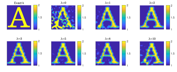
Figure 1: Test 1. The reconstructed coefficient $k(x)$, where the function $k(x)$ is given in (82) with $c_{a}=2$ inside of the letter ‘A’. We test different values of $\lambda$.

With $\lambda=3$, we display now in Figure 2 the convergence behavior of $|\nabla J_{\lambda,\beta}$ $(v$,$w$,$p$,$q)|$ with respect to the iterations of fmincon. We see that $|\nabla J_{\lambda,\beta}(v,w,p,q)|$ $\approx 0.01$ after 20 iterations. Then this value decreases very slowly with iterations. These justify the stopping criterion (86). We see on Figure 1 that with $\lambda=3$ the reconstructions of both the shape of the inclusion and the value of the contrast (84) are accurate ones.

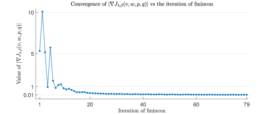
Figure 2: Test 1. The convergence of $|\nabla J_{\lambda,\beta}\left(v,w,p,q\right)|$ in the iteration of fmincon with $\lambda=3$ and the function $k(x)$ is given in (82) with $c_{a}=2$ inside of the letter ‘A’.

Test 2. We test the case when the inclusion in (82) has the shape of the letter ‘$A$’ for different values of the parameter $c_{a}=4,8$ inside of the letter ‘$A$’. Hence, by (83) the inclusion/background contrasts now are respectively $4:1$ and $8:1$. Computational results are displayed on Figure 3. One can observe that shapes of inclusions are imaged accurately. In addition, the computed inclusion/background contrasts (84) are accurate.

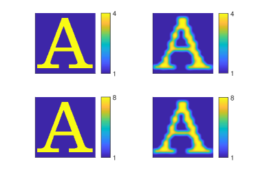
Figure 3: Test 2. Exact (left) and reconstructed (right) coefficient $k(x)$ with $c_{a}=4$ (first row) and $c_{a}=8$ (second row) inside of the letter ‘A’ as in (82). The inclusion/background contrasts in (83) are respectively $4:1$ and $8:1$. The reconstructions of both shapes of inclusions and the inclusion/background contrasts (84) are accurate.

Test 3. We test the case when the coefficient $k(x)$ in (82) has the shape of the letter ‘$\Omega$’ with $c_{a}=2$ inside of it. Results are presented on Figure 4. We again observe an accurate reconstruction.

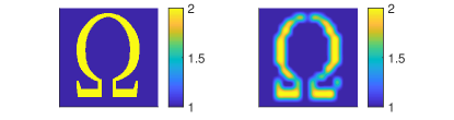
Figure 4: Test 3. Exact (left) and reconstructed (right) coefficient $k(x)$, where the function $k(x)$ is given in (82) with $c_{a}=2$ inside of the letter ‘$\Omega$’. The reconstructions of both the shape of the inclusions and the inclusion/background contrast (84) are accurate.

Test 4. We test the reconstruction for the case when the inclusion in (82) has the shape of two letters ‘SZ’ with $c_{a}=2$ in each of them. S and Z are two letters in the name of the city (Shenzhen) were the second author resides. The results are exhibited on Figure 5. Reconstructions of shapes of both letters as well as of the computed inclusions/background contrasts (84) in both letters are accurate ones.

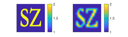
Figure 5: Test 4. Exact (left) and reconstructed (right) coefficient $k(x)$, where the function $k(x)$ is given in (82) with $c_{a}=2$ inside of two letters ‘SZ’. The reconstruction is worse than the one for the case of the single letter ‘$\Omega$’ in Figure 4. Nevertheless, the reconstructions of shapes of both letters are still accurate. In addition, the computed inclusion/background contrasts in (84) are accurately reconstructed in both letters.

Test 5. We consider the case when the random noisy is present in the data in (91) with $\delta=0.03$ and $\delta=0.05$, i.e. with 3% and 5% noise level. We test the reconstruction for the cases when the inclusion in (82) has the shape of either the letter ‘$A$’ or the letter ‘$\Omega$’ with $c_{a}=2$. The results are displayed on Figure 6. One can observe accurate reconstructions in all four cases. In particular, the inclusion/background contrasts in (84) are reconstructed accurately.

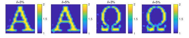
Figure 6: Test 5. Reconstructed coefficient $k(x)$ with the shape of letters ‘A’ or the letter ‘$\Omega$’ with $c_{a}=2$ from noisy data (91) with $\delta=0.03$ and $\delta=0.05$, i.e. with 3% and 5% noise level. In all these four cases, reconstructions of both shapes of inclusions and inclusion/background contrasts in (84) are accurate.

References

• [1] Y. Achdou, P. Cardaliaguet, F. Delarue, A. Porretta, and F. Santambrogio, Mean Field Games, vol. 2281 of Lecture Notes in Mathematics, C.I.M.E. Foundation Subseries, Springer Nature, Cetraro, Italy, 2019.
• [2] A. B. Bakushinskii, M. V. Klibanov, and N. A. Koshev, Carleman weight functions for a globally convergent numerical method for ill-posed Cauchy problems for some quasilinear PDEs, Nonlinear Analysis: Real World Applications, 34 (2017), pp. 201–224.
• [3] L. Baudouin, M. de Buhan, E. Crépeau, and J. Valein,  Carleman-based reconstruction algorithm on a wave network, available online, hal-04361363, (2023).
• [4] L. Baudouin, M. de Buhan, and S. Ervedoza, Convergent algorithm based on Carleman estimates for the recovery of a potential in the wave equation, SIAM J. Numer. Anal., 55 (2017), pp. 1578–1613.
• [5] L. Baudouin, M. de Buhan, S. Ervedoza, and A. Osses, Carleman-based reconstruction algorithm for the waves, SIAM J. Numer. Anal., 59 (2021), pp. 998–1039.
• [6] D. Bauso, H. Tembine, and T. Basar, Opinion dynamics in social networks through mean-field games, SIAM J. Control Optim, 54 (2016), pp. 3225–3257.
• [7] L. Beilina, Domain decomposition finite element/finite difference method for the conductivity reconstruction in a hyperbolic equation, Communications in Nonlinear Science and Numerical Simulation, 37 (2016), pp. 222–237.
• [8] L. Beilina and E. Lindström, An adaptive finite element/finite difference domain decomposition method for applications in microwave imaging, Electronics, 11 (2022), p. 1359.
• [9] A. L. Bukhgeim and M. V. Klibanov, Uniqueness in the large of a class of multidimensional inverse problems, Soviet Math. Doklady, 17 (1981), pp. 244–247.
• [10] Y. T. Chow, S. W. Fung, S. Liu, L. Nurbekyan, and S. Osher, A numerical algorithm for inverse problem from partial boundary measurement arising from mean field game problem, Inverse Problems, 39 (2022), p. 014001, https://doi.org/10.1088/1361-6420/aca5b0, https://doi.org/10.1088/1361-6420/aca5b0.
• [11] R. Couillet, S. M. Perlaza, H. Tembine, and M. Debbah, Electrical vehicles in the smart grid: A mean field game analysis, IEEE J. Sel. Areas Commun., 30 (2012), pp. 1086–1096.
• [12] L. Ding, W. Li, S. Osher, and W. Yin, A mean field game inverse problem, Journal of Scientific Computing, 92 (2022).
• [13] G. Giorgi, M. Brignone, R. Aramini, and M. Piana, Application of the inhomogeneous Lippmann–Schwinger equation to inverse scattering problems, SIAM J. Appl. Math., 73 (2013), pp. 212–231.
• [14] F. Gölgeleyen and M. Yamamoto, Stability for some inverse problems for transport equations, SIAM J. Math. Anal., 48 (2016), pp. 2319–2344.
• [15] A. V. Goncharsky, S. Y. Romanov, and S. Y. Seryozhnikov, On mathematical problems of two-coefficient inverse problems of ultrasonic tomography, Inverse Probl., 40 (2024), p. 045026.
• [16] M. Huang, P. E. Caines, and R. P. Malhamé, Large-population cost-coupled LQG problems with nonuniform agents: individual-mass behavior and decentralized Nash equilibria, IEEE Trans. Automat. Control, 52 (2007), pp. 1560–1571.
• [17] M. Huang, R. P. Malhamé, and P. E. Caines, Large population stochastic dynamic games: closed-loop McKean-Vlasov systems and the Nash certainty equivalence principle, Commun. Inf. Syst., 6 (2006), pp. 221–251.
• [18] O. Y. Imanuvilov, H. Liu, and M. Yamamoto, Lipschitz stability for determination of states and inverse source problem for the mean field game equations, Inverse Problems and Imaging, published online, (2024), https://doi.org/10.3934/ipi.2023057.
• [19] V. Isakov, Inverse Problems for Partial Differential Equations, Springer, New York, 2006.
• [20] M. V. Klibanov, Global convexity in a three-dimensional inverse acoustic problem, SIAM J. Math. Anal., 28 (1997), pp. 1371–1388.
• [21] M. V. Klibanov, Carleman estimates for global uniqueness, stability and numerical methods for coefficient inverse problems, J. Inverse Ill-Posed Probl., 21 (2013), pp. 477–510.
• [22] M. V. Klibanov, J. Li, and W. Zhang, Convexification for an inverse parabolic problem, Inverse Probl., 36 (2020), p. 085008.
• [23] M. V. Klibanov and J. Li, Inverse Problems and Carleman Estimates: Global Uniqueness, Global Convergence and Experimental Data, De Gruyter, Berlin, 2021.
• [24] M. V. Klibanov and Y. Averboukh, Lipschitz stability estimate and uniqueness in the retrospective analysis for the mean field games system via two Carleman estimates, SIAM J. Mathematical Analysis, 56 (2024), pp. 616–636.
• [25] M. V. Klibanov, A coefficient inverse problem for the mean field games system, Applied Mathematics and Optimization, 88 (2023), p. 54.
• [26] M. V. Klibanov, J. Li, and H. Liu, Hölder stability and uniqueness for the mean field games system via Carleman estimates, Studies in Applied Mathematics, 151 (2023), pp. 1447–1470.
• [27] M. V. Klibanov, J. Li, and Z. Yang, Convexification for a coefficient inverse problem for the mean field games system, arXiv: 2310.08878, (2023).
• [28] V. N. Kolokoltsov and O. A. Malafeyev, Many Agent Games in Socio-economic Systems: Corruption, Inspection, Coalition Building, Network Growth, Security, Springer Nature Switzerland AG, 2019.
• [29] O. A. Ladyzhenskaya, V. A. Solonnikov, and N. N. Uralceva, Linear and Quasilinear Equations of Parabolic Type, vol. 23, AMS, Providence, R.I., 1968.
• [30] J.-M. Lasry and P.-L. Lions, Jeux à champ moyen. i. le cas stationnaire., C. R. Math. Acad. Sci. Paris, 343 (2006), pp. 619–625.
• [31] J.-M. Lasry and P.-L. Lions, Mean field games, Japanese Journal of Mathematics, 2 (2007), pp. 229–260.
• [32] R. Y. Lay and Q. Li, Parameter reconstruction for general transport equation, SIAM J. Math. Anal., 52 (2020), pp. 2734–2758.
• [33] H. Liu, C. Mou, and S. Zhang, Inverse problems for mean field games, Inverse Probl., 39 (2023), p. 085003.
• [34] S. Ma and M. Salo, Fixed angle inverse scattering in the presence of a Riemannian metric, J. Inverse and Ill-Posed Problems, 30 (2022), pp. 495–520.
• [35] J. B. Malmberg and L. Beilina, An adaptive finite element method in quantitative reconstruction of small inclusions from limited observations, Appl. Math. Inf. Sci., 12 (2018), pp. 1–19.
• [36] R. G. Novikov, The $\bar{\partial}-$approach to approximate inverse scattering at fixed energy in three dimensions, International Math. Research Peports, 6 (2005), pp. 287–349.
• [37] Rakesh and M. Salo, The fixed angle scattering problem and wave equation inverse problems with two measurements, Inverse Problems, 36 (2020), p. 03500.
• [38] K. Ren, N. Soedjak, and K. Wang, Unique determination of cost functions in a multipopulation mean field game model, arXiv: 2312.01622, (2024).
• [39] V. G. Romanov, Inverse Problems of Mathematical Physics, VNU Press, Utrecht, The Netherlands, 1987.
• [40] A. N. Tikhonov, A. V. Goncharsky, V. V. Stepanov, and A. G. Yagola,  Numerical methods for the solution of Ill-posed problems, Kluwer, London, 1995.
• [41] N. V. Trusov, Numerical study of the stock market crises based on mean field games approach, J. Inverse Ill-Posed Probl., 29 (2021), pp. 849–865.
• [42] E. Weinan, H. Jiequn, and L. Qianxiao, A mean-field optimal control formulation of deep learning, Res. Math. Sci, 6 (2019), pp. 1–41.