Positional encoding is not the same as context: A study on positional encoding for Sequential recommendation

Abstract

The expansion of streaming media and e-commerce has led to a boom in recommendation systems, including Sequential recommendation systems, which consider the user’s previous interactions with items. In recent years, research has focused on architectural improvements such as transformer blocks and feature extraction that can augment model information. Among these features are context and attributes. Of particular importance is the temporal footprint, which is often considered part of the context and seen in previous publications as interchangeable with positional information. Other publications use positional encodings with little attention to them. In this paper, we analyse positional encodings, showing that they provide relative information between items that are not inferable from the temporal footprint. Furthermore, we evaluate different encodings and how they affect metrics and stability using Amazon datasets. We added some new encodings to help with these problems along the way. We found that we can reach new state-of-the-art results by finding the correct positional encoding, but more importantly, certain encodings stabilise the training.

1 Introduction

Sequential recommendation systems (SRS) have been booming within referral systems in the last few years since most of these systems are based on previous user behaviour and are present in almost all e-commerce, social media, and streaming platforms. Their effectiveness has led to various definitions of sequential recommendations and to their division into branches.

In general, sequential recommendation systems Fang et al. (2020), refer to recommendation systems (RS) where the interaction between the user and items is recorded sequentially. SRS are also related to session-based or session-aware recommendations. The latter two terms can be viewed as the sub-types of sequential recommendation when the interactions log is restricted to those made in the current session.

In this work, we adhere to the notation used in Fang et al. (2020) and use the term object to summarise the interactions. "Behavior object" means what the user interacts with, identified by an ID or a group of items. It may include text, images, and time. We will use "item(s)" for convenience. The interaction between items and users can use many different types of features. A typical split of those is attributes and context, where the attributes are features provided by the item, like a text description or an image, and the context refers to those features related to the interaction itself, like the time that a user tends to buy or search some streaming content.

A division based on the target task exists between the next-item recommendation and the next-basket recommendation Fang et al. (2020). In the next-item recommendation, a behaviour contains only one object (i.e., item), which could be a product, a song, a movie, or a location. In contrast, a behavior contains more than one object in next-basket recommendation.

When dealing with sequential systems, it is essential to consider the sequential nature of the data. Therefore, initial deep learning techniques utilised Convolutional Neural Networks (CNN) and Recurrent Neural Networks (RNN) to address this issue. However, attentional models have become increasingly popular due to their effectiveness, leading to multiple approaches utilising this technique Wang et al. (2021). Currently, most state-of-the-art models use attentional networks.

To summarise, our contribution is fourfold:

1. We analyse existing work and highlight that more than the standard usage of $5$ runs is needed to ensure the reliability of the results.

2. We propose new encodings. Based on our first experiments with existing encodings, we propose new encodings to improve metrics and stability.

3. We perform a detailed analysis of the types of encodings, their features (in-head, affected heads, etc.) and their ablations to see which factors improve the stability and the metrics.

4. We found correlations between the sparsity of the dataset and the encodings to get the best results. This precise data dependence, together with our study, provides a road map for the usage of encodings for SRS with transformer architectures.

2 Related Work

From an architectural perspective, SRS has evolved over the last two decades. Traditional methods in the field applied classic ML techniques, such as KNN for item-based systems (Davidson et al. (2010), Linden et al. (2003)), or applications of Markov Chains for different orders (He et al. (2017), He et al. (2016b), He and McAuley (2016a)). A common approach due to the sparsity of the interactions in RS is those based on matrix factorisation like DeepFM Guo et al. (2017) or CFM Xin et al. (2019). Among the different DL architectures, RNNs can capture sequence information and represent items based on their position in the list. One of the earliest and best known was Cho et al. (2014). The first approach from DL came using RNN, the most common architecture then. We can find models such as GRU4Rec Hidasi et al. (2016) or DREAM Yu et al. (2016). Another of the first approaches via DL was based on CNN models that can capture local features and consider time information in the input layer (Tang and Wang (2018), Tuan and Phuong (2017)). Among these were Caesar Li et al. (2021) and NextItNet Yuan et al. (2018). One of the first approaches using attention models was NARM Li et al. (2017), an encoder-decoder framework that uses attention at the bottleneck. The introduction of transformers and self-attention in sequential models came from AttRec Zhang et al. (2018).

Over time, different types of information have been identified to predict what a user might buy next. There are three main types of models for this: attribute-aware Rashed et al. (2022), context-aware Zhou et al. (2020), and time-aware Li et al. (2020). Attribute-aware models focus on the information provided by the items themselves. Context-aware models take into account the characteristics of the user’s interaction. Time-aware models are a subgroup of context-aware models that use the timing of the user’s interactions.

Using transformers in architecture has led to the introduction of positional embeddings. By default, the attention heads work like bags of tokens, and the positional information needs to be added to understand the sequential order of the tokens. Some approaches use time-aware information to replace the position, like in the case of CARCA Rashed et al. (2022). While this approach achieved excellent results, it faces some limitations. Replacing the positional embeddings with time stamps assumes that the order of the items will be implicitly deduced from this stamp. This can be more challenging to the model than simply an explicit representation. Furthermore, recent research in NLP Chen et al. (2021) has shown that introducing positional information within the attention, instead of the first head input, produces better results, which can not be done through the time stamps.

One of the first models considering the sequential information was GRU4Rec Hidasi et al. (2016), which concentrates on extracting information from the sequence of items instead of the user being an anonymous user model. A successful model from the context-aware point of view was DeepFM Guo et al. (2017), which extracted through the combination of factorisation models and deep learning extracts information from the context. Like GRU4Rec, using a self-attention layer to balance short-term intent and long-term preference can be found in SASRec Kang and McAuley (2018a). The extraction through a sequence of transformer encoders produces an output, which is compared with the target items through dot-product. This dot-product approach combines information from past behaviour and target representation, which was improved by an encoder-decoder architecture, where the encoder extracts past information, and the decoder combines the embedding representation for the target. This produced one of the SOTA models, CARCA Rashed et al. (2022). Another path of improvement from SASRec came from training the bidirectional transformer to infer the item-item relationship from the user’s historical interactions using the Cloze task in BERT4Rec Sun et al. (2019). Another one was TiSASRec Li et al. (2020), which further improves SASRec by considering time intervals between items.

We will focus on the position encoding applied to the most common datasets among these papers. For a deeper review of the different encoding techniques, one can see Zhao et al. (2024). Since there is no systematic study, each work addresses the encoding differently. In AttRec Zhang et al. (2018), they "furnish the query and key with time information by positional embeddings" using absolute embeddings. SASRec used absolute learnable position embeddings in the input sequence. They also tried the fixed position embedding as used in Vaswani et al. (2017) but found that this led to worse performance. In CARCA, which will be our base model, they tried using absolute encodings again, giving even worse results than no positional encoding. This disparity of results merits a more detailed analysis as in the present work.

3 Positional encodings

Encoding	Learnable	Type	Range	Layers	Concatenation	Integration
Abs	No	APE	Fix.	Vector Encoding	No	Add
Abs + Con	Yes	APE	Fix.	Vector Encoding	Yes	Joint
Rotatory	No	APE	Unl.	Vector Encoding	No	Multi.
Rotatory + Con.	Yes	APE	Unl.	Vector Encoding	Yes	Joint
RMHA-4	No	RPE	4	All	No	Multi.
Rope	No	APE	Unl.	All	No	Multi.
RopeOne	No	APE	Unl.	First	No	Multi.
Learnt	Yes	APE	Fix.	Vector Encoding	No	Add
Learnt + Con	Yes	APE	Fix.	Vector Encoding	Yes	Joint
None	No	N/A	N/A	0	N/A	N/A

Table 1: Encoding types: ’Type’ refers to absolute and relative. ’Learnable’ indicates whether the encoding parameters are learned during training. We also consider learnable to have a concatenation since there are learnable parameters. ’Range’ specifies the positions the encoding covers: ’Fix.’ fixed by the given length, ’Unl.’ means unlimited, while $4$ refers to the relative range. ’Layers’ represents the number of layers the encoding uses: "Vector Encoding" means they are added at the start by vectors (left in Fig: 1), All means in all the transformer blocks and First, at the first encoding block. ’Concatenation’ indicates whether there is a concatenation. ’Integration’ describes how the encoding is integrated with the model architecture: ’Add’ indicates a vector sum, ’Joint’ the concatenation, and ’Multi.’ for multiplication of matrices for those in the heads or element-wise for the others. Finally, None refers to no encoding.

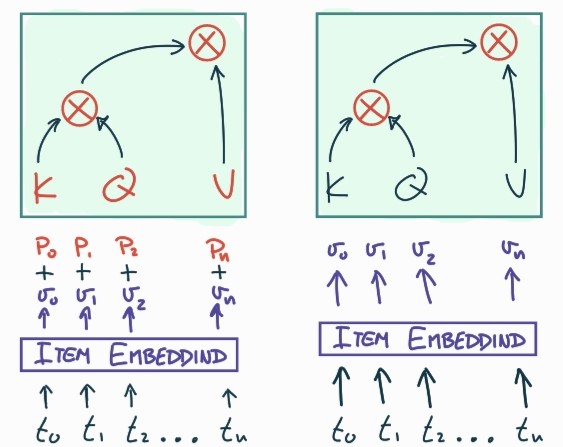
Figure 1: APE vs RPE : While APE encodings introduce the positional information as vectors before the $V$, $Q$ and $K$, projections, RPE add this information at the coefficient level in $K$ and $Q$. Parts affected by the position information appear in red.

3.1 Positional encodings

This section introduces the different types of encoding techniques used in this work. For a deeper review of the various encoding methods, check Zhao et al. (2024). Following Zhao et al. (2024), there are two prominent families of encoding methods. First, we have absolute positional encoding (APE ). These encodings are added before the first Transformer block, and the positional information provided is absolute, from the initial token to the last one. Second, there are the relative encoding methods (RPE ), which provide information about those items around the target item. These encodings are implemented inside the transformer’s head, more precisely in the Queries and Keys. In contrast to the common usage of encoding in Transformers for NLP tasks in RS, the encoding is reversed; the first item in the encoding order is the last one, and padding is applied on the left side Kang and McAuley (2018a). We chose this approach because the most relevant items are usually the ones that were recently visited or clicked. Due to the sinusoidal functions used in APE , the most pertinent items might be at the start because the assigned frequency becomes less distinguishable the later an item appears. We did some preliminary experiments to check if this is also right for another encoding, and the reversed encoding always produced better results, so in what follows, all the encoding will be considered as reversed.

Self-attention

enables models to weigh different parts of input sequences differently, allowing them to focus on relevant information during processing. The self-attention mechanism was introduced in Vaswani et al. (2017), which laid the foundation for the transformer architecture.

In self-attention, the input sequence is typically represented as a set of vectors, where each vector corresponds to a position in the sequence. This allows each position to attend to all other positions and captures dependencies and relationships within the sequence. For a given dimensionality $d$ of the item representation and a hidden dimension $H<d$, the attention weight assigned to each position is computed based on the similarity (dot product) between the query $Q\in\mathbb{R}^{d\times H}$, key $K\in\mathbb{R}^{d\times H}$, and value $V\in\mathbb{R}^{d\times H}$ matrices associated with the positions. These learnable matrices are derived from linear transformations of the original input $X\in\mathbb{R}^{n\times d}$ by multiplication, where $n$ is the number of items in the sequence.

The attention weight ($\alpha_{ij}$) assigned to position $i$ for attending to position $j$ is computed using the following formula:

$$\alpha_{ij}=\frac{{\exp((X_{i}\,Q)\cdot(X_{j}\,K)^{T}/\sqrt{d})}}{{\sum_{t=1}^{n}\exp((X_{i}\,Q)\cdot(X_{t}\,K)^{T}/\sqrt{d})}}$$ (1)

Here, $Q_{i}$ and $K_{j}$ represent the query and key matrices associated with positions $i$ and $j$, respectively. The dot product is scaled by $\sqrt{d}$ to prevent vanishing gradient problems. The resulting attention weights are then used to compute a weighted sum of the value matrices ($V_{j}$) associated with all positions:

$$\text{Attention}(Q,K,V)=\sum_{j=1}^{N}\alpha_{ij}X\cdot V_{j}$$ (2)

This weighted sum, representing the attended information, is then used as the output of the self-attention mechanism. The process is repeated for all positions in the sequence.

Absolute Positional Encoding (APE )

Absolute positional encoding adds fixed values to the embeddings of items based on their absolute position in the sequence. This means all the items have the same initial token as a reference. The most common approach is based on trigonometry, like in BERT Devlin et al. (2019), the so-called sinusoidal encoding. Absolute encoding is added at the input layer as part of the item encoding, 1. The most common practice is to add a vector encoding the position.

The absolute positional encoding for a token at position $i$ in a sequence of length $N$ can be calculated using trigonometric functions such as sine and cosine. A common formula is:

$$PE_{(pos,2i)}=\sin\left(\frac{{pos}}{{10000^{(2i/d)}}}\right)$$ (3)

$$PE_{(pos,2i+1)}=\cos\left(\frac{{pos}}{{10000^{(2i/d)}}}\right)$$ (4)

where $pos$ is the position of the item, $i$ is the dimension, and $d$ is the dimension of the embedding. This encoding is usually added to the original embedding, and we will refer to it along the text as absolute encoding (AE). For a given item embedding $x$ at position $pos$, we replace it as follows:

$$x=x+PE_{(pos,*)}$$ (5)

Another way of making the positional information more explicit and separated from the rest of the context and attributes is by concatenation, where we divide the dimension of the embedding into the context and attribute information and the positional encoding information:

$$x=Concat\,(x,PE_{(pos,*)})$$ (6)

We apply a Linear layer right after to recover the original dimension and do not change the number of parameters in the model. We will refer to them as concat absolute encoding (CAE). We added the position information orthogonally to make the model gradually rely on the position, producing more stable results, Section 5.

Learnable Encoding

Learnable position embeddings take a different approach by treating the positional information as parameters that can be updated during training. Instead of relying on predefined patterns, the model learns the optimal representation of positions based on the data context. We will denote these embeddings as learnable encoding (LE). In this case, we add a positional encoding, which is merely a learnable vector. We also apply a concatenation approach denoting as concatenated learnable encoding (CLE). In this case, their results will be generally worse than the classic residual connection.

Relative Positional Encoding (RPE )

A disadvantage of using APE is that it requires a fixed length of the input sequence and does not directly capture the relative positions of one item to another, whether the other is further ahead or backward. Relative position encoding (RPE ) was proposed to solve these issues, 1. Shaw et al. (2018) uses relative position encoding (RPE ) instead of APE and adds the position embeddings to the key and optional value projections instead of the input. A simplified version deleting the position embeddings in value projections in TranformersXL Dai et al. (2019) showed better performance on language modelling tasks. The length of the user’s session or action log varies significantly from user to user, suggesting that these encoding techniques may be of value to SRS.

The relative positional encoding can be computed using trainable parameters. The specific formula may depend on the implementation; in our case, we follow the one in Shaw et al. (2018), where the position is given inside the attention. The relation between two inputs $X_{i}$ and $X_{j}$ is given by $a_{ij}^{V},a_{ij}^{K}\in\mathbb{R}^{d_{a}}$, for values and keys. This information can be shared among heads, but we consider the case in which information is not shared.

For the relative case, the attention weight ($\alpha_{ij}$) can be written as:

$$\frac{{\exp((X_{i}\,Q)\cdot(X_{j}\,K+a_{ij}^{K})^{T}/\sqrt{d})}}{{\sum_{t=1}^{n}\exp((X_{i}\,Q)\cdot(X_{j}\,K+a_{ij}^{K})^{T}/\sqrt{d})}}$$ (7)

We also introduce the position at the value product as follows:

$$\text{Attention}(Q,K,V)=\sum_{j=1}^{N}\alpha_{ij}(X\cdot V_{j}+a_{ij}^{V})$$ (8)

Relative positional encoding can be especially useful when dealing with long sequences, as it allows the model to generalise better to different distances between items and in cases where the local position information is more critical. As a drawback, since it has to be applied to each attention head, it tends to be slower Shaw et al. (2018). We will denote these embeddings as RMHA-4 , where we bound the relative indexes to a distance of $4$. We do not apply a concatenated version in this case.

Rotary Encoding (Rope and Rotatory )

Unlike absolute or relative positional encoding, which focuses on representing positions in a fixed coordinate system or relative to other items in a sequence, rotary encoding leverages rotational transformations to encode position information. "Rotary Positional Encoding" typically refers to a specific technique used in positional encoding, Su et al. (2024). We will use the notation Rope to refer to them.

The motivation behind Rope is that the orientation or rotation of positional embeddings can provide valuable information about the relationship between items in a sequence. This approach is particularly relevant in scenarios where the inherent order or arrangement of items is not straightforward and can benefit from a more flexible representation, like a user searching for more than one item in the same session. These embeddings capture both linear order and rotational relationships within the sequence. Rotary position encodings apply a rotation to the Query and Key matrices, which preserves the dot product among the vectors.

In the two dimensional case for a given input vector $x$ the encoding function $f$ for given angle $\theta$ is defined as follows:

$$f_{\theta}(\mathbf{x})=\mathbf{R}(\theta)\cdot\mathbf{W}\cdot\mathbf{x}$$ (9)

Here, $\mathbf{R}(\theta)$ represents the rotation matrix parameterized by an angle $\theta$, expressed using sines and cosines, and $\mathbf{W}$ is either $K$ or $Q$. More explicit, for the $K$ case we have:

$$\begin{bmatrix}\cos(\theta)&-\sin(\theta)\\ \sin(\theta)&\cos(\theta)\end{bmatrix}\cdot\begin{bmatrix}K_{11}&K_{12}\\ K_{21}&K_{22}\end{bmatrix}\cdot\begin{bmatrix}x_{1}\\ x_{2}\end{bmatrix}$$ (10)

The straightforward generalisation of this to higher dimensionality divides the vector dimension into two-dimensional chunks and applies the rotation to each of them. Since this implementation is costly, the actual implementation expresses this rotation as two vector multiplications and one vector addition, as RoFormer Su et al. (2024).

Since we want to analyse the effect of the rotational position for sinusoidal, we propose here a new encoding, Rotatory , which is concatenated version Rotatory + Con. . Instead of directly applying sinusoidal functions, rotary encodings introduce an additional rotation mechanism by separating the angles into sine and cosine components and then alternating them across the embedding dimension. By alternating sine and cosine embeddings, the model can capture different phases of positional information, effectively introducing a rotational component to the encoding.

This rotation helps mitigate potential issues, such as vanishing gradients that can arise with traditional positional encoding, which is especially important for stability. So, while the term "rotary" might not directly imply physical rotation, it refers to the rotational mechanism introduced in the encoding process to enhance the representation of positional information in Transformer models. The implementation is similar to that from Rope , but applying the rotation matrices to the vector encodings added to the input items.

Dataset	Act	encoding	nmax	mean_hit	dev_hit	mean_ndcg	dev_ndcg
Beauty	silu	Rotatory-Longer	0.0001	61.87	1.04	42.60	0.98
Beauty	silu	Rotatory	0.0001	61.72	1.14	42.54	1.52
Beauty	silu	Rotatory + Con.	0.0001	61.68	1.04	42.31	0.97
Beauty	leaky	Rotatory + Con.	0.0001	61.16	0.77	42.83	0.48
Men	silu	RMHA-4-Longer	0.0001	70.13	0.42	46.41	4.18
Men	silu	RMHA-4	0.0001	69.70	0.64	43.75	1.44
Men	leaky	None	0.1000	69.69	1.28	57.94	1.69
Men	leaky	RMHA-4-Longer	0.0001	68.72	1.47	43.46	0.79
Fashion	silu	RMHA-4	0.0001	77.26	0.24	49.75	2.33
Fashion	silu	RMHA-4-Longer	0.0001	77.00	0.48	49.40	0.54
Fashion	leaky	RMHA-4	0.0001	76.46	0.25	49.49	2.18
Fashion	leaky	RMHA-4-Longer	0.0001	76.20	0.51	49.85	3.92
Games	leaky	Rotatory + Con.	NaN	80.62	0.55	56.07	0.79
Games	silu	Rotatory + Con.-Longer	NaN	80.29	0.47	55.18	0.55
Games	leaky	Rotatory + Con.-Longer	NaN	80.21	1.51	55.06	1.93
Games	silu	Learnt	NaN	79.82	1.88	54.30	2.95

Table 2: The table displays the top $4$ results for each dataset on cases with a standard deviation for $HIT$ below $3$.

Dataset	Act	encoding	nmax	mean_hit	dev_hit	mean_ndcg	dev_ndcg
Beauty	leaky	Abs + Con	0.0001	67.93	4.17	48.71	3.59
Beauty	silu	Learnt	0.0001	67.62	6.95	46.33	7.08
Beauty	silu	Abs	0.0001	67.27	10.59	45.34	10.75
Beauty	silu	Abs + Con	0.0001	65.87	5.23	45.61	5.12
Men	leaky	Learnt + Con	0.1000	73.86	7.18	58.89	8.15
Men	leaky	Learnt	0.0001	72.08	4.44	56.55	9.98
Men	leaky	Learnt + Con	0.0001	71.34	7.13	57.92	13.07
Men	leaky	Rotatory + Con.	0.1000	70.92	3.92	59.84	4.88
Fashion	silu	RMHA-4	0.0001	77.26	0.24	49.75	2.33
Fashion	silu	RMHA-4-Longer	0.0001	77.00	0.48	49.40	0.54
Fashion	leaky	RMHA-4	0.0001	76.46	0.25	49.49	2.18
Fashion	leaky	RMHA-4-Longer	0.0001	76.20	0.51	49.85	3.92
Games	leaky	Rotatory + Con.	NaN	80.62	0.55	56.07	0.79
Games	silu	Rotatory + Con.-Longer	NaN	80.29	0.47	55.18	0.55
Games	leaky	Rotatory + Con.-Longer	NaN	80.21	1.51	55.06	1.93
Games	silu	Learnt	NaN	79.82	1.88	54.30	2.95

Table 3: he table displays the top $4$ results for each dataset on cases with a standard deviation for HIT below $12$.

4 Experimental Setup

4.1 Datasets

We selected the Amazon dataset to assess the proficiency of various encoding types. For this purpose, we utilised four different real-world datasets extracted from product reviews on Amazon.com. These datasets have been diverse and widely used for SRS under the leave-one-out protocol (He and McAuley (2016b), Kang and McAuley (2018b), Hou et al. (2019), Wu et al. (2020), Steck (2019) and Zhou et al. (2020)). Since multiple versions of these datasets exist, we opted for the preprocessed versions from Rashed et al. (2022).

These datasets encompass various product categories, providing a diverse and comprehensive source for training and evaluating recommendation models. They provide essential features for each interaction, such as user IDs, item IDs, timestamps, and additional vector contextual information. As we can see in Tables 5, and 4, they provide diversity in the sparsity, which is going to be a key point in our analysis, but also on the discreteness of the features.

Dataset	Users	Items	Interactions	Attributes
Men	34,244	110,636	254,870	2,048
Fashion	45,184	166,270	358,003	2,048
Games	31,013	23,715	287,107	506
Beauty	52,204	57,289	394,908	6,507

Table 4: Dataset Statistics.

1.Beauty

(Wu et al. (2020), Zhou et al. (2020) and Kang and McAuley (2018b)) The dataset includes discrete and categorical attributes for all beauty products, including fine-grained categories and brands. Mainly categorical and discrete features.

2.Video Games

(Wu et al. (2020) and Kang and McAuley (2018b)) The Video Games sub-dataset includes user interactions, reviews, and product details specific to the video game category as price, brand and categorical features. Most of the attributes here are discrete and categorical.

3.Men

(He and McAuley (2016b)) The men’s dataset encompasses a comprehensive collection of items falling under men’s clothing. The attributes are dense vectors from image-based features extracted from the last layer of a ResNet50 Deng et al. (2009) on the ImageNet dataset He et al. (2016a).

3.Fashion

(He and McAuley (2016b) and Hou et al. (2019)) It contains 6 categories for men’s and women’s clothing. The features were extracted as dense using the same ResNet50 approach.

4.2 Models and Training

To implement CARCA, we converted TensorFlow code from the original model into Pytorch. We extracted the implementation in Papso (2023) for the part of the loss. The original version in TensorFlow was written on top of previous models written in TensorFlow. We found that these implementations check the metrics every $20$ epoch, assuming that the overfitting starts later. This is probably because some models need more than $1000$ epochs, and the cost of measurement becomes significant. We measure the metrics in a logarithmic manner, giving rise to slightly better results in some cases. Our implementation can be found here .

As in previous works (Rashed et al. (2022), Kang and McAuley (2018a), etc.), we use an ADAM optimiser to minimise the binary cross-entropy loss of the CARCA model while masking the padded items to prevent them from contributing to the loss function. For a given sequence of items interactions for a user $u$ as $\{i^{u}_{1},\ldots,i^{u}_{N}\}$, we create an input list as $I^{u+}=\{i^{u}_{1},\ldots,i^{u}_{N-1}\}$ by deleting the last item of the list, a positive target list as $T^{u+}=\{i^{u}_{2},\ldots,i^{u}_{N}\}$ by shifting one the input list, and a negative target list as $T^{u-}=\{i^{rand_{1}},\ldots,i^{rand_{N}-1}\}$ generated by random negative items. Then the loss is given by:

$$-\sum_{u\in U}\sum_{r\in T^{u+}\cup T^{u-}}\left[Y_{r}\log(\hat{Y}_{r})+(1-Y_{r})\log(1-\hat{Y}_{r})\right]$$

Here, $U$ represents the set of users, $T^{u+}\cup T^{u-}$ denotes the union of positive and negative items for user $u$, $Y_{r}$ is the observed interaction label for item $r$, and $\hat{Y}_{r}$ is the predicted probability of interaction with item $r$.

4.3 Metrics

We use two commonly used metrics for Next-Item Recommendations/SRS. Hit Rate measures the proportion of recommended items that overlap with the user’s actual interactions. Hit@10 counts the fraction of times the ground truth next item is among the top 10 items.

The second metric is Normalized Discounted Cumulative Gain (NDCG). NDCG considers the relevance of items and their positions in the recommended list.

$$NDCG=\frac{DCG}{IDCG}$$ (11)

Where $DCG$ (Discounted Cumulative Gain) is calculated as the sum of the relevance scores of items at each position in the ranked list, discounted by their position, and $IDCG$ (Ideal Discounted Cumulative Gain) represents the maximum possible $DCG$ for a perfect ranking.

$$DCG=\sum_{i=1}^{n}\frac{2^{rel_{i}}-1}{\log_{2}(i+1)}$$ (12)

$$IDCG=\sum_{i=1}^{n}\frac{2^{max(rel_{i},0)}-1}{\log_{2}(i+1)}$$ (13)

Here, $rel_{i}$ is the item’s relevance at position $i$ in the ranking.

5 Results

We present all the results for all the datasets and encodings in Appendix A.1. Due to space limitations, sub-tables were extracted from them.

Together with position encoding, we wanted to analyse other factors that could affect stability. In CARCA Rashed et al. (2022), they found $0.0001$ as the best upper bound ($nmax$ in our Tables) for the encoding vectors in all the datasets except for Games. We try different maximum values for all the encoding vectors ($0.1$ and $0.0001$) to see if their choice depends on the encoding. Except for some exceptions, the upper bound $0.0001$ produces better results. We also tried the activation function $silu$ instead of the $leakyrelu$. The results are slightly better regarding stability but without a strong correlation.

5.1 Stability

A common practice among the papers is to present an average of $5$. Our first experiments showed a significant difference between each one of the runs. We decided to analyse the deviation for the different trainings. The deviation and mean can be found in all the training tables. We also decided to compute the $95\%$ significance confidence interval and present it with the confidence interval in the complete tables results in Appendix A.1.

Inter-Dataset Deviation:

The stability varies from one dataset to another, being the Beauty dataset the most stable with an average Hit deviation of $0.9$ and NDCG deviation of $0.87$. Meanwhile, the maximum deviations are obtained by fashion. We can see that those datasets with a lower sparsity tend to be more stable, as do the Beauty and Games datasets, while those with a higher sparsity are less stable, as are the Men and Fashion datasets.

Inter-Encoding Deviation:

In Table 6 and Table 12 in the Appendix, we see that some encodings produce more stable results than others. More precisely, the concatenated version for Abs , Learnt and Rotatory + Con. generally present more stable results. Furthermore, for the more stable case of $0.0001$ upper bound, in Table 6, Abs and Learnt are still significantly stable. At the same time, our Rotatory encoding produces similar results to the concatenated version. This could be because the average deviation is similar to no encoding, None . The most notable case is RMHA-4 , which, combined with the upper bound $0.0001$, gives the most stable results, around $0.51$, compared with the no-encoding case, $2.36$. This pattern is preserved to the general upper bound, suggesting that this encoding provides excellent stability. As we will see below, this encoding is worth trying in cases of high sparsity.

Encoding Ablation:

We can appreciate that Learnt and the sinusoidal Abs tend to have a similar deviation, higher than not using any encoding. To know if the stability is provided by the fact that RMHA-4 introduce positional information in each transformer or being a RPE head, we trained Rope . The results show that it is a mid between RMHA-4 on the one hand and Learnt and Abs on the other hand. It does not add or reduce stability for None . We wanted to know if being Rope in a middle point is due to being in all the transformer blocks while not being a APE encoding. To this goal, we added RopeOne , an ablation which applies Rope but only in the first block. The results are not far away from each other. We can see in Table 12 that RopeOne is even slightly better, while in Table 6, they are almost the same, in this case, slightly worse. Then, we decided to create a new encoding, Rotatory , which uses the rotatory properties but is not in the attention heads but a vector encoding. The results show the same stability as Rope and its ablation.

The stability of the RMHA-4 encoding can also be appreciated in the losses. In Appendix A.5.

Dataset	Hit Dev.	NDCG Dev.	CI-length	Density/Sparsity-1
Men	3.9143	8.2742	5.6686	$6.727\times 10^{-}5$
Fashion	4.87	9.7814	9.2257	$4.765\times 10^{-}5$
Games	1.124	0.952	1.616	$3.904\times 10^{-}4$
Beauty	0.935	0.87	1.22	$1.320\times 10^{-}4$

Table 5: Deviations among the different datasets without Encoding. This pattern is generally preserved along the different encodings.

encoding	dev HIT	dev NDCG	runs	CI-length
Abs	5.43	8.25	9.38	6.71
Abs + Con	3.52	5.56	7.12	5.35
Learnt	4.79	7.64	7.88	7.05
Learnt + Con	3.17	6.36	6.62	4.42
None	2.35	5.26	8.00	3.29
RMHA-4	0.51	1.08	6.00	0.88
Rope	2.38	5.45	5.00	4.04
Rotatory	2.46	5.01	8.38	3.48
Rotatory + Con.	2.48	5.18	6.75	3.49
RopeOne	2.82	6.54	4.29	5.46
Rope-Longer	3.33	8.15	5.25	5.99
Rotatory-Longer	1.05	1.04	4.67	2.08
Rotatory + Con.-Longer	0.99	1.24	6.00	1.59
RMHA-4-Longer	0.71	4.00	6.00	1.14

Table 6: Deviations among the different encodings. Relative encoding in all the heads, RMHA-4 , presents more stability.

5.2 Best Results

Which is the best encoding?

It depends on the spacing and the definition that one manages to get a good result. If we look at the table 7, we see that this dataset has excellent stability, but in cases like Learnt with $0.1$, with leakyrelu, the model gets over $74$ in HIT, but the $95\%$ confidence interval is ($60.74$, $88.24$). In other words, applying this approach cements the results of what was studied here Picard (2021); in some cases, it is better to get a good set of seeds than a suitable method.

Maximum deviation of $12$:

If we consider a maximum of $12$ as deviation, we get Table 3. In CARCA, they did an ablation study on the Men Dataset, showing that using Abs moves towards worse results. They produced similar results for Men, but both had a deviation of around $6$, so the results from the ablation were more a matter of initialisation. In this case, Men and Beauty get their best results with Learnt -like and Abs -like encodings, respectively. But they are unstable. In contrast, Fashion and Games get their top values with RMHA-4 and Rotatory , respectively, which are stable.

Maximum deviation of $3$:

If we reduce the maximum deviation to $3$, we get some results that we consider the right results. As we can see in Table 2, the best encodings are RMHA-4 and Rotatory (or its concatenated version), and they correlate with the sparsity. Those with a high sparsity benefit more from the extra stability provided by RMHA-4 , while those with a lower sparsity, Beauty and Games, get their best through a purely rotatory approach Rotatory . We can see that even considering only those which are stable, the results obtained in all the datasets are new SOTA.

Encoding "Ablation":

We created some ablations from existing encoding techniques to analyse where the stability came from. So far, our experiments used almost the same hyperparameters as the original CARCA. Looking again at the losses, we found that some of the top results did not converge, i.e., the loss and the metrics were improving. Thus, we decided to extend some trainings with more epochs to see if this produced better results. We added $400$ epochs to the default values (11). The improvements were not significant in this regard.

6 Conclusion

Our main conclusion is that encodings should not be considered minor in this model family. On the contrary, they are a powerful tool, and depending on the data set, a couple of possible better choices can be pre-selected. We have shown that the higher the sparsity, the better the results, as they stabilise the training until the best results are achieved. On the other hand, when the set density is sufficient, our rotatory encodings are a good choice or a learnable encoding. Also, at publication time, we have achieved SOTA results using only the encodings. And these results are, in most cases, more reliable than previous SOTA results.

7 Future work

During the encoding analysis, we found some correlation between the bound used for the encoding and the stability. Previous works have experimented with very low bounds, usually below $0.001$. We would like to go deep in this direction and analyse the behaviour of the metric used for encoding and its bounds.

8 Limitations

Despite the details of this study, it was carried out using a transformer architecture. Today, the latest models in the field are based on this architecture or GCNs. Using other architectures may affect this study and the conclusions on using encodings. The fact that the choice depends on the dataset can give a first idea of the possible encodings in case of using different architectures.

Appendix A Appendix

A.1 Experiments

In this section, we present all our results for the four datasets, thereby completing the missing experiments from the sub-tables in the main corpus. In tables 7, 8, and 9, we can find Rope-Longer , which is not presented in Table 1. These are just a few cases in which we extend the number of epochs since we found that for Rope , it takes longer to reach its maximum.

Act	encoding	nmax	mean_hit	dev_hit	mean_ndcg	dev_ndcg	runs	CI	CI-length
leaky	None	0.0001	56.00	0.96	37.93	0.65	9	(55.37, 56.63)	1.26
silu	None	0.0001	57.03	0.83	38.42	0.68	9	(56.49, 57.57)	1.08
leaky	None	0.1000	49.02	1.18	30.73	1.21	9	(48.25, 49.79)	1.54
silu	None	0.1000	49.69	0.77	31.35	0.94	9	(49.19, 50.19)	1.00
leaky	Learnt + Con	0.0001	56.36	0.65	37.94	1.54	3	(55.62, 57.1)	1.48
silu	Learnt + Con	0.0001	56.69	0.51	37.82	0.65	3	(56.11, 57.27)	1.16
leaky	Learnt + Con	0.1000	49.29	0.71	30.98	0.99	3	(48.49, 50.09)	1.60
silu	Learnt + Con	0.1000	49.85	1.18	31.42	1.48	3	(48.51, 51.19)	2.68
leaky	Abs + Con	0.0001	67.93	4.17	48.71	3.59	5	(64.27, 71.59)	7.32
silu	Abs + Con	0.0001	65.87	5.23	45.61	5.12	5	(61.29, 70.45)	9.16
leaky	Abs + Con	0.1000	51.42	1.41	32.10	0.46	3	(49.82, 53.02)	3.20
silu	Abs + Con	0.1000	54.54	3.33	35.43	3.34	5	(51.62, 57.46)	5.84
leaky	Rotatory + Con.	0.0001	61.16	0.77	42.83	0.48	3	(60.29, 62.03)	1.74
silu	Rotatory + Con.	0.0001	61.68	1.04	42.31	0.97	3	(60.5, 62.86)	2.36
leaky	Rotatory + Con.	0.1000	50.51	1.59	32.25	1.76	3	(48.71, 52.31)	3.60
silu	Rotatory + Con.	0.1000	50.88	1.00	32.70	0.87	3	(49.75, 52.01)	2.26
leaky	Learnt	0.0001	59.83	3.71	39.85	3.11	3	(55.63, 64.03)	8.40
silu	Learnt	0.0001	67.62	6.95	46.33	7.08	5	(61.53, 73.71)	12.18
leaky	Learnt	0.1000	74.49	17.19	51.36	22.65	6	(60.74, 88.24)	27.50
silu	Learnt	0.1000	61.75	7.84	40.02	7.34	10	(56.89, 66.61)	9.72
silu	Rotatory-Longer	0.0001	61.87	1.04	42.60	0.98	2	(60.43, 63.31)	2.88
silu	Rotatory-Longer	0.1000	49.33	2.08	30.89	2.28	2	(46.45, 52.21)	5.76
leaky	Abs	0.0001	63.65	8.36	43.68	8.36	13	(59.11, 68.19)	9.08
silu	Abs	0.0001	67.27	10.59	45.34	10.75	15	(61.91, 72.63)	10.72
leaky	Abs	0.1000	57.25	10.84	37.65	10.73	12	(51.12, 63.38)	12.26
silu	Abs	0.1000	61.23	15.24	39.14	11.78	16	(53.76, 68.7)	14.94
leaky	RMHA-4	0.0001	56.29	0.81	37.66	1.14	3	(55.37, 57.21)	1.84
silu	RMHA-4	0.0001	57.00	0.35	37.22	0.32	3	(56.6, 57.4)	0.80
leaky	RMHA-4	0.1000	51.30	0.32	33.38	0.15	3	(50.94, 51.66)	0.72
silu	RMHA-4	0.1000	51.35	0.42	33.04	0.12	3	(50.87, 51.83)	0.96
leaky	RopeOne	0.0001	55.33	1.22	37.89	1.24	3	(53.95, 56.71)	2.76
silu	RopeOne	0.0001	57.25	1.16	38.76	1.01	3	(55.94, 58.56)	2.62
leaky	RopeOne	0.0001	55.95	0.21	38.41	0.65	3	(55.71, 56.19)	0.48
silu	RopeOne	0.0001	56.23	0.63	37.69	0.55	3	(55.52, 56.94)	1.42
leaky	Rope	0.0001	56.30	0.92	38.60	0.82	3	(55.26, 57.34)	2.08
silu	Rope	0.0001	56.59	0.72	37.21	0.98	3	(55.78, 57.4)	1.62
leaky	Rope	0.1000	50.04	0.80	31.91	0.89	3	(49.13, 50.95)	1.82
silu	Rope	0.1000	49.15	0.71	31.31	1.01	3	(48.35, 49.95)	1.60
leaky	Rotatory	0.0001	58.69	1.31	40.83	0.71	5	(57.54, 59.84)	2.30
silu	Rotatory	0.0001	61.72	1.14	42.54	1.52	5	(60.72, 62.72)	2.00
leaky	Rotatory	0.1000	49.11	1.17	30.57	1.28	5	(48.08, 50.14)	2.06
silu	Rotatory	0.1000	49.40	0.96	31.14	1.04	5	(48.56, 50.24)	1.68

Table 7: Beauty results with different positional encodings. Original results from Rashed et al. (2022) at the end.

Act	encoding	nmax	mean_hit	dev_hit	mean_ndcg	dev_ndcg	runs	CI	CI-length
leaky	None	0.0001	65.44	3.54	46.46	9.99	9	(63.13, 67.75)	4.62
silu	None	0.0001	70.38	1.82	53.34	7.00	6	(68.92, 71.84)	2.92
leaky	None	0.1000	54.04	7.99	38.82	9.53	3	(45.0, 63.08)	18.08
silu	None	0.1000	61.53	11.84	48.13	14.97	3	(48.13, 74.93)	26.80
leaky	Learnt + Con	0.0001	69.31	7.74	50.73	12.02	14	(65.26, 73.36)	8.10
silu	Learnt + Con	0.0001	69.81	2.03	49.49	7.59	7	(68.31, 71.31)	3.00
leaky	Learnt + Con	0.1000	65.29	7.61	52.91	9.70	10	(60.57, 70.01)	9.44
silu	Learnt + Con	0.1000	66.15	7.47	50.59	9.46	14	(62.24, 70.06)	7.82
leaky	Abs + Con	0.0001	67.30	4.48	52.26	9.94	10	(64.52, 70.08)	5.56
silu	Abs + Con	0.0001	70.83	1.64	59.93	1.95	6	(69.52, 72.14)	2.62
leaky	Abs + Con	0.1000	64.93	10.58	52.21	13.11	16	(59.75, 70.11)	10.36
silu	Abs + Con	0.1000	65.14	8.20	51.71	11.06	13	(60.68, 69.6)	8.92
leaky	Rotatory + Con.	0.0001	69.13	2.80	55.33	7.69	9	(67.3, 70.96)	3.66
silu	Rotatory + Con.	0.0001	71.16	1.38	48.61	8.62	7	(70.14, 72.18)	2.04
leaky	Rotatory + Con.	0.1000	68.61	2.76	57.08	3.72	7	(66.57, 70.65)	4.08
silu	Rotatory + Con.	0.1000	65.23	7.76	52.99	9.31	11	(60.64, 69.82)	9.18
leaky	Learnt	0.0001	68.37	5.75	51.41	12.43	13	(65.24, 71.5)	6.26
silu	Learnt	0.0001	67.63	5.75	46.36	11.95	13	(64.5, 70.76)	6.26
leaky	Learnt	0.1000	64.99	9.00	47.66	14.48	16	(60.58, 69.4)	8.82
silu	Learnt	0.1000	63.94	9.49	46.44	10.58	16	(59.29, 68.59)	9.30
leaky	RMHA-4-Longer	0.0001	76.20	0.51	49.85	3.92	6	(75.79, 76.61)	0.82
silu	RMHA-4-Longer	0.0001	77.00	0.48	49.40	0.54	6	(76.62, 77.38)	0.76
leaky	Rope-Longer	0.0001	68.63	3.97	51.05	11.71	5	(65.15, 72.11)	6.96
silu	Rope-Longer	0.0001	71.50	1.22	49.69	6.41	7	(70.6, 72.4)	1.80
leaky	Abs	0.0001	66.39	4.61	51.99	9.51	10	(63.53, 69.25)	5.72
silu	Abs	0.0001	69.52	4.76	49.72	10.39	10	(66.57, 72.47)	5.90
leaky	Abs	0.1000	59.75	9.74	44.73	12.86	15	(54.82, 64.68)	9.86
silu	Abs	0.1000	58.39	8.48	41.86	11.31	15	(54.1, 62.68)	8.58
leaky	RMHA-4	0.0001	76.46	0.25	49.49	2.18	6	(76.26, 76.66)	0.40
silu	RMHA-4	0.0001	77.26	0.24	49.75	2.33	6	(77.07, 77.45)	0.38
leaky	RMHA-4	0.1000	60.63	5.14	40.75	8.06	11	(57.59, 63.67)	6.08
silu	RMHA-4	0.1000	63.61	4.41	39.48	7.97	11	(61.0, 66.22)	5.22
leaky	RopeOne	0.0001	73.03	6.52	62.96	8.59	3	(65.65, 80.41)	14.76
silu	RopeOne	0.0001	71.70	1.82	51.07	11.17	3	(69.64, 73.76)	4.12
leaky	RopeOne	0.0001	69.27	5.02	54.24	11.80	6	(65.25, 73.29)	8.04
silu	RopeOne	0.0001	70.49	1.66	49.17	10.70	6	(69.16, 71.82)	2.66
leaky	Rope	0.0001	66.73	4.81	47.49	12.62	5	(62.51, 70.95)	8.44
silu	Rope	0.0001	71.40	1.75	52.83	8.88	5	(69.87, 72.93)	3.06
leaky	Rope	0.1000	61.24	8.78	48.13	10.86	6	(54.21, 68.27)	14.06
silu	Rope	0.1000	62.79	8.79	49.27	10.69	8	(56.7, 68.88)	12.18
leaky	Rotatory	0.0001	68.95	2.90	53.66	9.58	15	(67.48, 70.42)	2.94
silu	Rotatory	0.0001	70.87	1.22	48.23	7.43	15	(70.25, 71.49)	1.24
leaky	Rotatory	0.1000	62.02	10.97	48.79	13.69	18	(56.95, 67.09)	10.14
silu	Rotatory	0.1000	62.68	8.53	49.41	10.86	15	(58.36, 67.0)	8.64
leaky	None	0.0001	59.1	–	38.1	–	5	–	–

Table 8: Fashion Dataset results with different positional encodings. Original results from Rashed et al. (2022) at the end.

Act	encoding	nmax	mean_hit	dev_hit	mean_ndcg	dev_ndcg	runs	CI	CI-length
leaky	None	0.0001	65.19	6.37	48.99	11.96	9	(61.03, 69.35)	8.32
silu	None	0.0001	64.90	3.06	47.51	9.84	6	(62.45, 67.35)	4.90
leaky	None	0.1000	69.69	1.28	57.94	1.69	3	(68.24, 71.14)	2.90
silu	None	0.1000	65.66	0.89	53.12	0.67	3	(64.65, 66.67)	2.02
leaky	Learnt + Con	0.0001	71.34	7.13	57.92	13.07	7	(66.06, 76.62)	10.56
silu	Learnt + Con	0.0001	66.64	4.49	48.38	12.61	7	(63.31, 69.97)	6.66
leaky	Learnt + Con	0.1000	73.86	7.18	58.89	8.15	7	(68.54, 79.18)	10.64
silu	Learnt + Con	0.1000	62.18	7.83	47.82	10.83	7	(56.38, 67.98)	11.60
leaky	Abs + Con	0.0001	70.84	5.13	57.63	9.89	9	(67.49, 74.19)	6.70
silu	Abs + Con	0.0001	65.55	4.59	49.37	10.61	6	(61.88, 69.22)	7.34
leaky	Abs + Con	0.1000	67.31	6.18	54.49	9.17	9	(63.27, 71.35)	8.08
silu	Abs + Con	0.1000	63.33	7.50	48.62	10.54	9	(58.43, 68.23)	9.80
leaky	Rotatory + Con.	0.0001	70.64	5.29	59.30	6.98	10	(67.36, 73.92)	6.56
silu	Rotatory + Con.	0.0001	67.18	5.82	50.27	13.21	10	(63.57, 70.79)	7.22
leaky	Rotatory + Con.	0.1000	70.92	3.92	59.84	4.88	6	(67.78, 74.06)	6.28
silu	Rotatory + Con.	0.1000	63.88	7.42	50.69	9.75	10	(59.28, 68.48)	9.20
leaky	Learnt	0.0001	72.08	4.44	56.55	9.98	7	(68.79, 75.37)	6.58
silu	Learnt	0.0001	66.18	7.81	46.61	11.21	8	(60.77, 71.59)	10.82
leaky	Learnt	0.1000	67.71	9.94	49.97	9.10	8	(60.82, 74.6)	13.78
silu	Learnt	0.1000	67.15	12.19	51.53	14.44	8	(58.7, 75.6)	16.90
leaky	RMHA-4-Longer	0.0001	68.72	1.47	43.46	0.79	3	(67.06, 70.38)	3.32
silu	RMHA-4-Longer	0.0001	70.13	0.42	46.41	4.18	6	(69.79, 70.47)	0.68
leaky	Rope-Longer	0.0001	68.74	4.59	56.80	5.87	4	(64.24, 73.24)	9.00
silu	Rope-Longer	0.0001	67.31	3.54	51.40	8.62	5	(64.21, 70.41)	6.20
leaky	Abs	0.0001	65.46	6.64	50.75	11.48	9	(61.12, 69.8)	8.68
silu	Abs	0.0001	64.15	2.94	42.68	8.87	6	(61.8, 66.5)	4.70
leaky	Abs	0.1000	69.20	4.78	54.43	8.87	6	(65.38, 73.02)	7.64
silu	Abs	0.1000	65.30	8.34	52.33	10.38	9	(59.85, 70.75)	10.90
leaky	RMHA-4	0.0001	68.65	0.48	43.24	0.35	6	(68.27, 69.03)	0.76
silu	RMHA-4	0.0001	69.70	0.64	43.75	1.44	6	(69.19, 70.21)	1.02
leaky	RMHA-4	0.1000	58.72	3.28	41.22	6.16	6	(56.1, 61.34)	5.24
silu	RMHA-4	0.1000	60.77	1.59	40.89	5.90	6	(59.5, 62.04)	2.54
leaky	RopeOne	0.0001	69.77	7.86	54.24	17.65	3	(60.88, 78.66)	17.78
silu	RopeOne	0.0001	62.14	0.74	37.49	3.31	3	(61.3, 62.98)	1.68
leaky	RopeOne	0.0001	67.82	6.59	54.10	12.14	6	(62.55, 73.09)	10.54
silu	RopeOne	0.0001	66.24	4.18	49.30	11.44	6	(62.9, 69.58)	6.68
leaky	Rope	0.0001	65.29	6.06	49.86	11.15	7	(60.8, 69.78)	8.98
silu	Rope	0.0001	63.93	3.25	46.10	7.61	5	(61.08, 66.78)	5.70
leaky	Rope	0.1000	62.76	9.47	49.77	12.13	6	(55.18, 70.34)	15.16
silu	Rope	0.1000	61.24	8.88	46.52	12.55	6	(54.13, 68.35)	14.22
leaky	Rotatory	0.0001	67.71	5.57	52.99	11.95	9	(64.07, 71.35)	7.28
silu	Rotatory	0.0001	67.07	3.63	54.88	4.54	6	(64.17, 69.97)	5.80
leaky	Rotatory	0.1000	68.07	4.68	56.31	6.21	6	(64.33, 71.81)	7.48
silu	Rotatory	0.1000	63.07	8.92	49.38	12.30	10	(57.54, 68.6)	11.06
leaky	None	0.0001	55.0	–	34.9	–	5	–	–

Table 9: Men Dataset results with different positional encodings. Original results from Rashed et al. (2022) at the end.

Act	encoding	nmax	mean_hit	dev_hit	mean_ndcg	dev_ndcg	runs	CI	CI-length
leaky	None	NaN	78.95	1.25	53.37	1.21	6	(77.95, 79.95)	2.00
silu	None	NaN	78.49	0.98	52.83	0.74	10	(77.88, 79.1)	1.22
leaky	Learnt + Con	NaN	78.34	1.28	54.14	1.39	6	(77.32, 79.36)	2.04
silu	Learnt + Con	NaN	79.32	1.50	53.68	1.97	6	(78.12, 80.52)	2.40
leaky	Rotatory + Con.	NaN	80.62	0.55	56.07	0.79	6	(80.18, 81.06)	0.88
silu	Rotatory + Con.	NaN	79.61	2.17	54.80	2.71	6	(77.87, 81.35)	3.48
leaky	Abs + Con	NaN	79.71	1.28	54.93	1.50	6	(78.69, 80.73)	2.04
silu	Abs + Con	NaN	79.34	1.67	54.23	1.84	10	(78.3, 80.38)	2.08
leaky	Learnt	NaN	78.64	2.05	54.30	2.41	6	(77.0, 80.28)	3.28
silu	Learnt	NaN	79.82	1.88	54.30	2.95	8	(78.52, 81.12)	2.60
leaky	Rotatory + Con.-Longer	NaN	80.21	1.51	55.06	1.93	6	(79.0, 81.42)	2.42
silu	Rotatory + Con.-Longer	NaN	80.29	0.47	55.18	0.55	6	(79.91, 80.67)	0.76
leaky	Rotatory-Longer	NaN	78.00	1.10	52.30	1.05	6	(77.12, 78.88)	1.76
silu	Rotatory-Longer	NaN	76.41	1.00	51.48	1.10	6	(75.61, 77.21)	1.60
leaky	Abs	NaN	75.27	2.30	49.61	2.90	6	(73.43, 77.11)	3.68
silu	Abs	NaN	73.27	3.25	47.22	3.75	6	(70.67, 75.87)	5.20
leaky	RMHA-4	NaN	78.85	0.51	53.32	0.44	12	(78.56, 79.14)	0.58
silu	RMHA-4	NaN	76.59	0.78	51.54	0.43	6	(75.97, 77.21)	1.24
leaky	RopeOne	NaN	78.82	0.62	53.45	0.42	6	(78.32, 79.32)	1.00
silu	RopeOne	NaN	78.27	1.19	52.85	0.88	6	(77.32, 79.22)	1.90
leaky	Rope	NaN	78.97	0.33	53.64	0.27	6	(78.71, 79.23)	0.52
silu	Rope	NaN	77.56	1.17	52.04	1.25	6	(76.62, 78.5)	1.88
leaky	Rotatory	NaN	76.56	2.17	51.09	2.29	6	(74.82, 78.3)	3.48
silu	Rotatory	NaN	76.21	1.77	51.06	2.04	6	(74.79, 77.63)	2.84
leaky	None	0.0001	78.2	–	57.3	–	5	–	–

Table 10: Games Dataset results with different positional encodings. Original results from Rashed et al. (2022) at the end.

A.2 Resources

Due to the instability of these models, we had to run many seeds to get some confident results. We started by running each one of the model configurations three times. After that, we decided to run more seeds based on the confidence of each one of the cases. We tried to keep at least a confidence range of ten points. We used $V100$ GPUs of 32GBs. For $men$ and $fashion$, based on the encoding, the training times go from $4$ to $6$ hours. For $Beauty$, they went from $22$ to $26$ hours. Based on the team’s resource ability, these experiments were carried out over $6$ months, lasting between $1$ and $8$.

We used the following seeds: $42$, $43$, $44$, $45$, $46$, $1809$, $1810$, $1811$, $1812$, $1741$, $1742$, $1743$, $1744$, $1745$, $123$, $234$, $345$, $456$, $567$, $678$, $789$, $890,102$, $203$, $304$, $405$, $506$, $607$, $708$, $808$, $901$, $1001$, $987$, $8765$, $7654$, and $6543$.

A.3 Hyperparameters

In this section, we present the hyperparameters used for training. As mentioned above, we use the same hyperparameters as CARCA Rashed et al. (2022). In some cases, we experimented with the upper bound from the norm in the encoding and the training length.

Hyperparameter	Men	Fashion	Games	Beauty
Learning Rate	0.000006	0.00001	0.0001	0.0001
Max Seq. Length	35	35	50	75
Number of attention blocks	3	3	3	3
Number of attention heads	3	3	3	1
Dropout Rate	0.3	0.3	0.5	0.5
L2 reg. weight	0.0001	0.0001	0	0.0001
Embedding Dimension d	390	390	90	90
Embedding Dimension g	1950	1950	450	450
Residual connection in the cross-attention block	No	No	Yes	Yes

Table 11: Hyperparameters with corresponding options were used in the original CARCA model. This parameter were written in tensor flow. In "L2 reg. weight", the value $0$ corresponds to no bound, which in Pytorch is $Nan$, and we denote it as None .

A.4 Deviations over all the trainings

Here, we present the table with all the deviation values from the training. In the table in the main text, we considered those training where we use the default values for the upper bound, i.e., $0.0001$, and $None$ for the Games dataset. We can see that the trends pointed out in Section 5.1 are still valid in this table. The encodings with concatenation are more stable, and RMHA-4 is the most stable one. We can see that with longer trainings Rotatory encodings become more stable than Rope

encoding	HIT dev	NDCG dev	runs	CI-length
Abs	7.20	9.42	10.57	8.42
Abs + Con	4.67	6.58	8.00	6.36
Learnt	7.43	9.98	9.07	10.17
Learnt + Con	4.09	6.53	6.93	5.66
None	3.05	5.08	6.71	5.62
RMHA-4	1.37	2.64	6.29	1.98
Rope	4.03	6.55	5.14	6.52
Rotatory	3.92	6.10	9.00	4.92
Rotatory + Con.	3.16	5.12	6.71	4.47
RopeOne	2.82	6.54	4.29	5.46
Rope-Longer	3.33	8.15	5.25	5.99
Rotatory-Longer	1.31	1.35	4.00	3.00
Rotatory + Con.-Longer	0.99	1.24	6.00	1.59
RMHA-4-Longer	0.71	4.00	6.00	1.14

Table 12: Deviations among the different encodings. Those per head, like RMHA-4 or Rope , are more stable than others.

A.5 Losses

This section shows some loss cases from our trainings showing the stability of RMHA-4 . The first image shows four test losses for $0.0001$ as upper bound, with silu activation. The first row corresponds to the None encoding, while the second row is the RMHA-4 encoding. Each row contains the losses of four different seeds. The seeds are not paired vertically but randomly selected.

The second image shows the validation Losses for the analogous case in the Men Dataset.

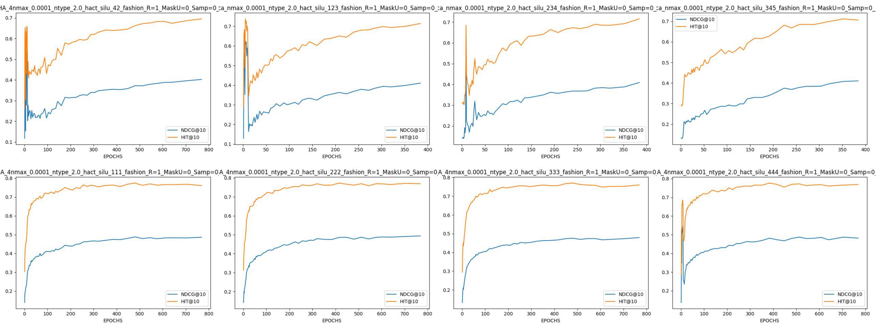
Figure 2: Losses randomly selected from None , first row, and RMHA-4 , second row, for the test set with $0.0001$ ad silu. Dataset: Fashion

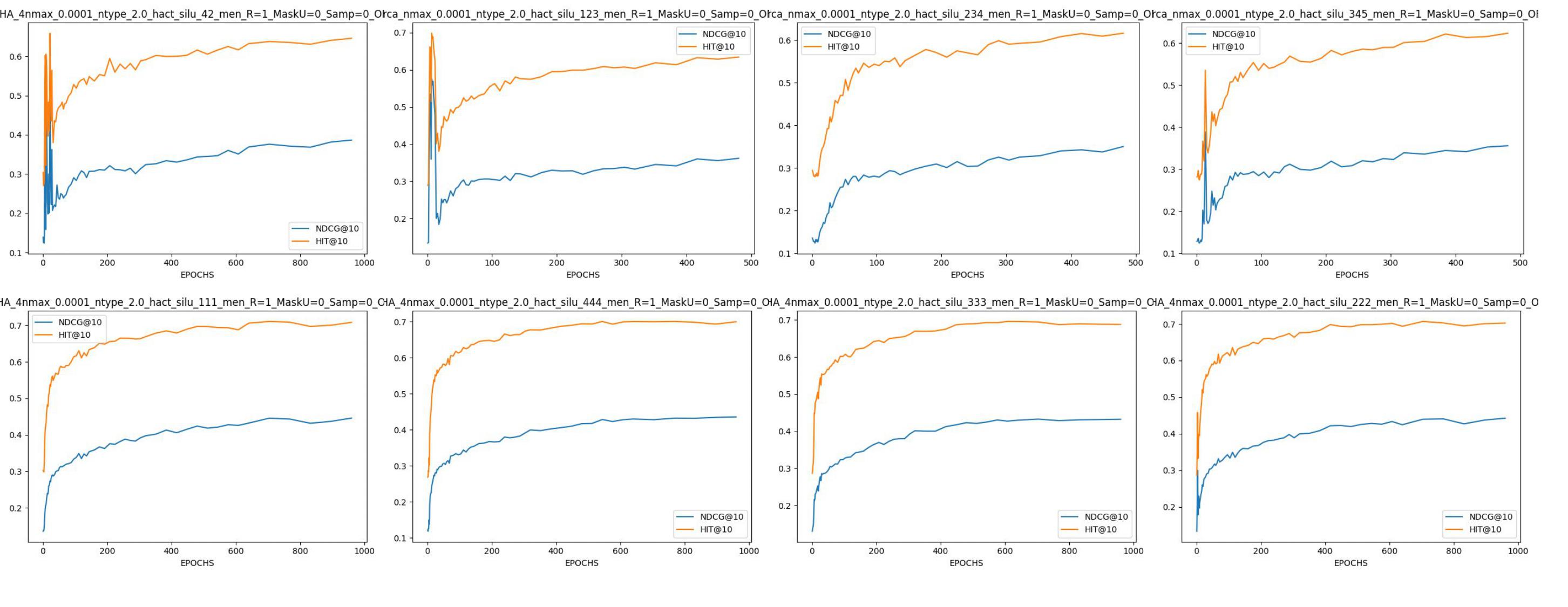
Figure 3: Losses randomly selected from None , first row, and RMHA-4 , second row, for the test set with $0.0001$ ad silu. Dataset: Men

References

- Chen et al. (2021) Pu-Chin Chen, Henry Tsai, Srinadh Bhojanapalli, Hyung Won Chung, Yin-Wen Chang, and Chun-Sung Ferng. 2021. A simple and effective positional encoding for transformers. In Proceedings of the 2021 Conference on Empirical Methods in Natural Language Processing, pages 2974–2988, Online and Punta Cana, Dominican Republic. Association for Computational Linguistics.
- Cho et al. (2014) Kyunghyun Cho, Bart van Merrienboer, Dzmitry Bahdanau, and Yoshua Bengio. 2014. On the properties of neural machine translation: Encoder-decoder approaches.
- Dai et al. (2019) Zihang Dai, Zhilin Yang, Yiming Yang, Jaime Carbonell, Quoc Le, and Ruslan Salakhutdinov. 2019. Transformer-XL: Attentive language models beyond a fixed-length context. In Proceedings of the 57th Annual Meeting of the Association for Computational Linguistics, pages 2978–2988, Florence, Italy. Association for Computational Linguistics.
- Davidson et al. (2010) James Davidson, Benjamin Liebald, Junning Liu, Palash Nandy, Taylor Van Vleet, Ullas Gargi, Sujoy Gupta, Yu He, Mike Lambert, Blake Livingston, and Dasarathi Sampath. 2010. The youtube video recommendation system. In Proceedings of the Fourth ACM Conference on Recommender Systems, RecSys ’10, page 293–296, New York, NY, USA. Association for Computing Machinery.
- Deng et al. (2009) Jia Deng, Wei Dong, Richard Socher, Li-Jia Li, Kai Li, and Li Fei-Fei. 2009. Imagenet: A large-scale hierarchical image database. In 2009 IEEE Conference on Computer Vision and Pattern Recognition, pages 248–255.
- Devlin et al. (2019) Jacob Devlin, Ming-Wei Chang, Kenton Lee, and Kristina Toutanova. 2019. BERT: Pre-training of deep bidirectional transformers for language understanding. In Proceedings of the 2019 Conference of the North American Chapter of the Association for Computational Linguistics: Human Language Technologies, Volume 1 (Long and Short Papers), pages 4171–4186, Minneapolis, Minnesota. Association for Computational Linguistics.
- Fang et al. (2020) Hui Fang, Danning Zhang, Yiheng Shu, and Guibing Guo. 2020. Deep learning for sequential recommendation: Algorithms, influential factors, and evaluations. ACM Trans. Inf. Syst., 39(1).
- Guo et al. (2017) Huifeng Guo, Ruiming Tang, Yunming Ye, Zhenguo Li, and Xiuqiang He. 2017. Deepfm: A factorization-machine based neural network for ctr prediction. In Proceedings of the 26th International Joint Conference on Artificial Intelligence, IJCAI’17, page 1725–1731. AAAI Press.
- He et al. (2016a) Kaiming He, Xiangyu Zhang, Shaoqing Ren, and Jian Sun. 2016a. Deep residual learning for image recognition. In 2016 IEEE Conference on Computer Vision and Pattern Recognition (CVPR), pages 770–778.
- He et al. (2016b) Ruining He, Chen Fang, Zhaowen Wang, and Julian McAuley. 2016b. Vista: A visually, socially, and temporally-aware model for artistic recommendation. In Proceedings of the 10th ACM Conference on Recommender Systems, RecSys ’16. ACM.
- He et al. (2017) Ruining He, Wang-Cheng Kang, and Julian McAuley. 2017. Translation-based recommendation. In Proceedings of the Eleventh ACM Conference on Recommender Systems, RecSys ’17, page 161–169, New York, NY, USA. Association for Computing Machinery.
- He and McAuley (2016a) Ruining He and Julian McAuley. 2016a. Fusing similarity models with markov chains for sparse sequential recommendation. In 2016 IEEE 16th International Conference on Data Mining (ICDM), pages 191–200.
- He and McAuley (2016b) Ruining He and Julian McAuley. 2016b. Vbpr: visual bayesian personalized ranking from implicit feedback. In Proceedings of the Thirtieth AAAI Conference on Artificial Intelligence, AAAI’16, page 144–150. AAAI Press.
- Hidasi et al. (2016) Balázs Hidasi, Alexandros Karatzoglou, Linas Baltrunas, and Domonkos Tikk. 2016. Session-based recommendations with recurrent neural networks.
- Hou et al. (2019) Min Hou, Le Wu, Enhong Chen, Zhi Li, Vincent W. Zheng, and Qi Liu. 2019. Explainable fashion recommendation: A semantic attribute region guided approach. In Proceedings of the Twenty-Eighth International Joint Conference on Artificial Intelligence, IJCAI-19, pages 4681–4688. International Joint Conferences on Artificial Intelligence Organization.
- Kang and McAuley (2018a) Wang-Cheng Kang and Julian McAuley. 2018a. Self-attentive sequential recommendation. In 2018 IEEE International Conference on Data Mining (ICDM), pages 197–206.
- Kang and McAuley (2018b) Wang-Cheng Kang and Julian McAuley. 2018b. Self-attentive sequential recommendation.
- Li et al. (2020) Jiacheng Li, Yujie Wang, and Julian McAuley. 2020. Time interval aware self-attention for sequential recommendation. In Proceedings of the 13th International Conference on Web Search and Data Mining, WSDM ’20, page 322–330, New York, NY, USA. Association for Computing Machinery.
- Li et al. (2017) Jing Li, Pengjie Ren, Zhumin Chen, Zhaochun Ren, Tao Lian, and Jun Ma. 2017. Neural attentive session-based recommendation. In Proceedings of the 2017 ACM on Conference on Information and Knowledge Management, CIKM ’17, page 1419–1428, New York, NY, USA. Association for Computing Machinery.
- Li et al. (2021) Lei Li, Li Chen, and Ruihai Dong. 2021. Caesar: context-aware explanation based on supervised attention for service recommendations. Journal of Intelligent Information Systems, 57(1):147–170. Publisher Copyright: © 2020, Springer Science+Business Media, LLC, part of Springer Nature. Copyright: Copyright 2020 Elsevier B.V., All rights reserved.
- Linden et al. (2003) G. Linden, B. Smith, and J. York. 2003. Amazon.com recommendations: item-to-item collaborative filtering. IEEE Internet Computing, 7(1):76–80.
- Papso (2023) Rastislav Papso. 2023. Complementary product recommendation for long-tail products. In Proceedings of the 17th ACM Conference on Recommender Systems, RecSys ’23, page 1305–1311, New York, NY, USA. Association for Computing Machinery.
- Picard (2021) David Picard. 2021. Torch.manual_seed(3407) is all you need: On the influence of random seeds in deep learning architectures for computer vision.
- Rashed et al. (2022) Ahmed Rashed, Shereen Elsayed, and Lars Schmidt-Thieme. 2022. Context and attribute-aware sequential recommendation via cross-attention. In Proceedings of the 16th ACM Conference on Recommender Systems, RecSys ’22, page 71–80, New York, NY, USA. Association for Computing Machinery.
- Shaw et al. (2018) Peter Shaw, Jakob Uszkoreit, and Ashish Vaswani. 2018. Self-attention with relative position representations. In Proceedings of the 2018 Conference of the North American Chapter of the Association for Computational Linguistics: Human Language Technologies, Volume 2 (Short Papers), pages 464–468, New Orleans, Louisiana. Association for Computational Linguistics.
- Steck (2019) Harald Steck. 2019. Embarrassingly shallow autoencoders for sparse data. CoRR, abs/1905.03375.
- Su et al. (2024) Jianlin Su, Murtadha Ahmed, Yu Lu, Shengfeng Pan, Wen Bo, and Yunfeng Liu. 2024. Roformer: Enhanced transformer with rotary position embedding. Neurocomputing, 568:127063.
- Sun et al. (2019) Fei Sun, Jun Liu, Jian Wu, Changhua Pei, Xiao Lin, Wenwu Ou, and Peng Jiang. 2019. Bert4rec: Sequential recommendation with bidirectional encoder representations from transformer. In Proceedings of the 28th ACM International Conference on Information and Knowledge Management, CIKM ’19, page 1441–1450, New York, NY, USA. Association for Computing Machinery.
- Tang and Wang (2018) Jiaxi Tang and Ke Wang. 2018. Personalized top-n sequential recommendation via convolutional sequence embedding. CoRR, abs/1809.07426.
- Tuan and Phuong (2017) Trinh Xuan Tuan and Tu Minh Phuong. 2017. 3d convolutional networks for session-based recommendation with content features. In Proceedings of the Eleventh ACM Conference on Recommender Systems, RecSys ’17, page 138–146, New York, NY, USA. Association for Computing Machinery.
- Vaswani et al. (2017) Ashish Vaswani, Noam Shazeer, Niki Parmar, Jakob Uszkoreit, Llion Jones, Aidan N. Gomez, Łukasz Kaiser, and Illia Polosukhin. 2017. Attention is all you need. In Proceedings of the 31st International Conference on Neural Information Processing Systems, NIPS’17, page 6000–6010, Red Hook, NY, USA. Curran Associates Inc.
- Wang et al. (2021) Shoujin Wang, Yan Wang, Quan Sheng, Mehmet Orgun, Longbing Cao, and Defu Lian. 2021. A survey on session-based recommender systems. ACM Computing Surveys, 2021:39.
- Wu et al. (2020) Liwei Wu, Shuqing Li, Cho-Jui Hsieh, and James Sharpnack. 2020. Sse-pt: Sequential recommendation via personalized transformer. In Proceedings of the 14th ACM Conference on Recommender Systems, RecSys ’20, page 328–337, New York, NY, USA. Association for Computing Machinery.
- Xin et al. (2019) Xin Xin, Bo Chen, Xiangnan He, Dong Wang, Yue Ding, and Joemon Jose. 2019. Cfm: Convolutional factorization machines for context-aware recommendation. In Proceedings of the Twenty-Eighth International Joint Conference on Artificial Intelligence, IJCAI-19, pages 3926–3932. International Joint Conferences on Artificial Intelligence Organization.
- Yu et al. (2016) Feng Yu, Qiang Liu, Shu Wu, Liang Wang, and Tieniu Tan. 2016. A dynamic recurrent model for next basket recommendation. In Proceedings of the 39th International ACM SIGIR Conference on Research and Development in Information Retrieval, SIGIR ’16, page 729–732, New York, NY, USA. Association for Computing Machinery.
- Yuan et al. (2018) Fajie Yuan, Alexandros Karatzoglou, Ioannis Arapakis, Joemon M. Jose, and Xiangnan He. 2018. A simple convolutional generative network for next item recommendation. Proceedings of the Twelfth ACM International Conference on Web Search and Data Mining.
- Zhang et al. (2018) Shuai Zhang, Yi Tay, Lina Yao, Aixin Sun, and Jake An. 2018. Next item recommendation with self-attentive metric learning.
- Zhao et al. (2024) Liang Zhao, Xiaocheng Feng, Xiachong Feng, Dongliang Xu, Qing Yang, Hongtao Liu, Bing Qin, and Ting Liu. 2024. Length extrapolation of transformers: A survey from the perspective of positional encoding.
- Zhou et al. (2020) Kun Zhou, Hui Wang, Wayne Xin Zhao, Yutao Zhu, Sirui Wang, Fuzheng Zhang, Zhongyuan Wang, and Ji-Rong Wen. 2020. S3-rec: Self-supervised learning for sequential recommendation with mutual information maximization. In Proceedings of the 29th ACM International Conference on Information & Knowledge Management, CIKM ’20, page 1893–1902, New York, NY, USA. Association for Computing Machinery.