Describing heat dissipation in the resistive state of three-dimensional superconductors

Abstract

In this work we study the role of the heat diffusion equation in simulating the resistive state of superconducting films. By analyzing the current-voltage and current-resistance characteristic curves for temperatures close to $T_{c}$ and various heat removal scenarios, we demonstrate that heat diffusion notably influences the behavior of the resistive state, specially near the transition to the normal state, where heat significantly changes the critical current and the calculated resistance. Furthermore, we show how the efficiency of the substrate has important effects in the dynamics of the system, particularly for lower temperatures. Finally, we investigate the hysteresis loops, the role of the film thickness and of the Ginzburg-Landau parameter, the findings reassuring the significance of accounting for heat diffusion in accurately modeling the resistive state of superconducting films and provide valuable insights into its complex dynamics. To accomplish these findings, we have used the $3D$ generalized Ginzburg-Landau equation coupled with the heat diffusion equation.

[inst1]organization=Departamento de Física, Faculdade de Ciências, Universidade Estadual Paulista (UNESP),addressline=Av. Eng. Edmundo Carrijo Coube, 14-01, city=Bauru, postcode=17033-360, state=São Paulo, country=Brazil

Four sequential frames depicting the evolution of a vortex-antivortex pair in a superconductor, from nucleation at the borders to annihilation at the center. The pair traverses the $yz$ plane, intersecting both the lower and upper $xy$ planes. The left and right columns display the color maps for the order parameter and temperature, respectively. It can be observed that as the vortex-antivortex penetrates deeper into the superconductor, the temperature correspondingly increases.

It is introduced a numerical method that enables the study of heat diffusion in three-dimensional superconductors.

It is investigated how heat removal efficiency affects the critical properties of the resistive state of three-dimensional superconductors.

It is shown how parameters such as the film thickness and the Ginzburg-Landau parameter affects the heat diffusion process.

1 Introduction

Throughout the years, superconductivity has remained a highly significant and influential subject within the field of condensed matter physics. The study of superconducting phenomena continues to yield insights and practical applications. One intriguing aspect of superconductivity pertains to the resistive state that emerges under certain conditions. Specifically, the self-field of the transport current in superconductors can lead to a resistive state [1, 2, 3, 4, 5]. In type-II superconductors, the circularly shaped magnetic self-field induced by a current gives rise to Abrikosov vortices with ring-like shapes, commonly referred to as closed vortices [6].

In recent decades, the advancement of superconducting devices has been facilitated by the evolution in experimental techniques. These devices are frequently operated by applying currents, a practice that has prompted an intensified analysis of superconducting samples under such conditions [1, 2, 4, 7, 8]. Among the pivotal considerations in this domain, the interplay of heat diffusion and the superconducting properties of these systems stands out. As the devices progressively shrink in size, their susceptibility to thermal effects also amplifies. The current flow through these superconducting structures has the potential to induce resistive heating due to the intrinsic electrical resistance of materials, even when they are in the superconducting state. This resistive heating can give rise to the generation of heat within the device. Thus, the heat diffusion properties inherent in these nanoscale superconducting systems take an undeniable importance to the very functioning of the device itself [9, 10, 11].

In Ref. [9], for instance, the authors explore the Joule heating produced by the motion of vortices through conformal-mapped nanoholes. The asymmetric distribution of nanoholes causes a vortex motion dependent on the polarity of the current. The disparity in the dissipated heat between the two current directions gives rise to a superconducting diode. It is thus clear that a correct description of heat dispersion becomes indispensable for the modeling and perfection of such devices.

In Ref. [10] the authors applied a theoretical analysis employing a numerical solution that encompassed the coupled time-dependent Ginzburg-Landau and heat dissipation equations. This analysis showed a relationship between critical currents and the applied magnetic field within a mesoscopic square structure outfitted with attached contacts. In line with experimental findings, the study elucidated the presence of hysteresis phenomena. These hysteresis effects were ascribed to the substantial heat dissipation occurring within the sample, particularly at current levels that approached the depairing Ginzburg-Landau threshold or were influenced by the dynamic behavior of the superconducting condensate.

In a previous work of Ref. [6] the authors investigated the resitive state of a long superconducting film. We describe a crossover phenomenon where straight vortex-antivortex (v-av) pairs transition to curved (closed) v-av pairs as the thickness of the superconducting film increases. We establish a criteria for this transition based on the aspect ratio of the vortex and show that it correlates with changes in the IV curve. An indirect method for detecting closed vortices experimentally has been proposed. This method involves measuring the time-averaged magnetic flux at the lateral sides of the film. In this paper we will extend this work, now investigating how the three-dimensional dynamics of the closed v-av pairs affects the heat diffusion of the superconducting system.

Therefore, the main objective of this study is to investigate the impact of the heat diffusion properties on the resistive state of mesoscopic superconductors with finite thickness, within a fully three-dimensional model. In particular, we aim to explore how the behavior of superconducting samples, with varying thicknesses and applied currents, is influenced by different substrate properties. To achieve this, we consider the effect of temperature fluctuations on the resistive state, thus providing a view of how substrate properties and temperature interplay in the behavior of mesoscopic superconductors.

Moreover, in the above above cited works, the heat diffusion process was studied within a two-dimensional framework, which it is the common practice in the literature. While the $2D$ model is capable of capturing the qualitative features of the vortex dynamics, we show here that critical parameters, such as the critical currents to the onset of the resistive and normal states, obtained by the $2D$ model significantly differs fro the ones obtained within the fully $3D$ model developed in this work. These findings are relevant to future simulations aiming the proposal of novel superconducting devices, where the precise knowledge of the critical parameters of the system are of great importance.

The outline of this paper is as follows. In Section 2 we present a comprehensive overview of the theoretical model, encompassing the generalized Ginzburg-Landau equation coupled with Ampere’s law and heat diffusion equation which are essential to describe the resistive state of superconductors. In Section 3, we detail the methodology, covering the employed parameters and the numerical techniques utilized to solve these equations. The remaining of this Section is devoted to presenting both the results and discussion. In Section 4 we present our concluding remarks.

2 The Theoretical Model

To investigate the evolution of superconductivity in a dirty superconductor, we use the framework of the generalized time-dependent Ginzburg-Landau (GTDGL) equation, [12, 13] coupled with the Ampère’s law. The equations are written as:

$$\frac{u}{\sqrt{1+\gamma^{2}|\psi|^{2}}}\left[\frac{\partial}{\partial t}+\mbox{i}\varphi+\frac{1}{2}\gamma^{2}\frac{\partial|\psi|^{2}}{\partial t}\right]\psi=$$

$$=-\left(-\mbox{\mbox{i}\boldmath$\nabla$}-\textbf{A}\right)^{2}\psi+\psi(1-T-|\psi|^{2}),$$ (1)

$$\sigma\left(\frac{\partial\textbf{A}}{\partial t}+\mbox{\boldmath$\nabla$}\varphi\right)=\textbf{J}_{s}-\kappa^{2}\mbox{\boldmath$\nabla$}\times\textbf{h},$$ (2)

where

$$\textbf{J}_{s}={\rm Re}\left[\bar{\psi}{(-\mbox{\mbox{i}\boldmath$\nabla$}-\textbf{A})}\psi\right]$$ (3)

is the superconducting current density.

To obtain the scalar potential in each time instant, we use the equation for the continuity of electric charge:

$$\frac{\partial\rho}{\partial t}+\mbox{\boldmath$\nabla$}\cdot\textbf{J}=0$$ (4)

where $\rho$ is the electric charge density and the total current J can be decomposed as the sum of the superconducting current $\textbf{J}_{s}$ and the normal current $\textbf{J}_{n}=\sigma\textbf{E}$, with the electric field being written as:

$$\textbf{E}=-\frac{\partial\textbf{A}}{\partial t}-\mbox{\boldmath$\nabla$}\varphi.$$ (5)

Replacing Eq. (5) into Eq. (4) and assuming there is no charge accumulation, that is $\partial\rho/\partial t=0$, we obtain:

$$\nabla^{2}\varphi=\frac{1}{\sigma}\mbox{\boldmath$\nabla$}\cdot\textbf{J}_{s},$$ (6)

where we have also adopted the Coulomb gauge $\mbox{\boldmath$\nabla$}\cdot\textbf{A}=0$.

Here, Eqs. (1-6) are written in dimensionless units, where the temperature $T$ is in units of the critical temperature $T_{c}$; the order parameter $\psi$ is in units of $\psi_{\infty}(0)=\sqrt{\alpha(0)/\beta}$, where $\alpha$ and $\beta$ are two phenomenological constants; the distances are measured in units of the coherence length at zero temperature $\xi(0)$; the vector potential A is in units of $H_{c2}(0)\xi(0)$, where $H_{c2}(0)$ is the upper critical field at zero temperature; the local magnetic field $\textbf{h}=\mbox{\boldmath$\nabla$}\times\textbf{A}$ is in units of $H_{c2}(0)$; the current density is in units of $J_{GL}=\sigma\hbar/2e\xi(0)t_{GL}$ and we use $I_{GL}=J_{GL}\xi^{2}(0)$ as units of total current; time is in units of the Ginzburg-Landau characteristic time $t_{GL}=\xi^{2}(0)/D$, where $D$ is the diffusion coefficient; the scalar potential is units of $\varphi_{GL}=H_{c2}(0)D/c$; the material dependent parameter $\gamma=2\tau_{E}\Delta_{0}/\hbar$, where $\tau_{E}$ is the inelastic electron-collision time, and $\Delta_{0}$ is the gap in the Meissner state; $\kappa=\lambda(0)/\xi(0)$ is the Ginzburg-Landau parameter, where $\lambda(0)$ is the London penetration depth at zero temperature; the normal state electrical conductivity $\sigma$ is in units of $c^{2}/4\pi D\kappa^{2}$; and finally, the constant $u$ is equal to 5.79, which is derived from first principles [12].

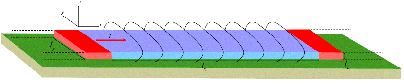
Figure 1: (Color online) Schematic view of a superconductor film (blue) with dimensions specified in the figure. The red region symbolizes a metallic film carrying a certain current that is injected (ejected) into the superconductor through two contacts, similar to a NSN junction. All these elements are on the top of a substrate (green).

Additionally, to take into account the effects of the heat produced in the process of creation and annihilation of vortices, we couple the GTDGL equation with the heat diffusion equation [10] given by:

$$\mathcal{C}\frac{\partial T}{\partial t}=\zeta\nabla^{2}T+W$$ (7)

where $\mathcal{C}$ is the effective heat capacity, $\zeta$ is the effective heat conductivity coefficient. In this work, we have used $\mathcal{C}=0.03$ and $\zeta=0.06$. The term $W$ represents the power dissipated by the system. For gap superconductor it is given by [14, 15, 16]:

$$\leavevmode\resizebox{325.215pt}{}{$W=\sigma\textbf{E}^{2}+\frac{u}{\sqrt{1+\gamma^{2}|\psi|^{2}}}\left[\left|\frac{\partial\psi}{\partial t}\right|^{2}+\frac{\gamma^{2}}{4}\left(\frac{\partial|\psi|^{2}}{\partial t}\right)^{2}\right]$},$$ (8)

which is the generalization of the expression first determined for gapless superconductor in Ref. [17]. Eqs. 1, 2, 6, and 7 must solved to obtain the order parameter, the scalar and vector potentials and the local temperature.

Fig. 1 illustrates the system under investigation, which consists of a long film with a central cutout representing a superconductor with dimensions ($l_{x},l_{y},l_{z}$) (blue region). On both the right and left sides, two long metallic films (red regions) are present, where a fixed current density, denoted by $J_{a}$, is applied. The total current injected (or ejected) at the metallic contacts is expressed by $I=l_{y}l_{z}J_{a}$. Essentially, we have a NSN junction (normal metal - superconductor - normal metal), on top of a substrate (green region). To study solely the effects of temperature, we alter the system size according to the bath temperature $T_{0}$, the confinement being the same for all cases. For all temperatures, the dimensions are the same in units of $\xi(T)$, the values being $l_{x}=12\xi(T)$, $l_{y}=8\xi(T)$ and $l_{z}=1.2\xi(T)$, where $\xi(T)=\xi(0)/\sqrt{1-T/T_{c}}$. For example, for $T_{0}=0.75T_{c}$, we have $l_{x}=24\xi(0)$, $l_{y}=16\xi(0)$ and $l_{z}=2.4\xi(0)$.

The external current is introduced in the system through the boundary conditions for the scalar potential. At the superconductor/normal contact interfaces the scalar potential obeys $\hat{\textbf{n}}\cdot\mbox{\boldmath$\nabla$}\varphi=-J_{a}$, where $\hat{\textbf{n}}$ is the unit vector perpendicular to the interface and $J_{a}$ is the applied current density. At the remaining interfaces, we have $\hat{\textbf{n}}\cdot\mbox{\boldmath$\nabla$}\varphi=0$.

To guarantee the superconducting current does not leave the stripe, the following condition must be imposed to the order parameter at the boundaries of the system:

$$\hat{\textbf{n}}\cdot(-\mbox{i}\mbox{\boldmath$\nabla$}-\bm{A})\psi=\frac{\mbox{i}}{b}\psi\,,$$ (9)

where $b$ is the de Gennes extrapolation length; here $b$ is set to be equal to $20$ at the superconductor/normal contact interfaces and goes to infinity at the other interfaces.

At all interfaces of the $3D$ system, the local magnetic field h is equal to the magnetic field H produced by an uniform current density flowing in the superconducting film. This field is given by:

$$\kappa^{2}\mbox{\boldmath$\nabla$}\times\textbf{H}=J_{a}\hat{\textbf{x}}\,.$$ (10)

The solution of this equation can be found in the supplementary material of Ref. [5]. Here, we must emphasize that, by using the solution of Eq. 10 as our boundary conditions for the local field, we are disregarding demagnetization effects at the boundaries of the system. This approximation is a necessity driven by the considerable computational demands associated with solving the Ampère’s law in the surrounding regions of the superconducting system to obtain the stray fields. Although this is fully justified only for large values of $\kappa$, the qualitative features remain unchanged even for $\kappa\approx 1$.

Finally, we must specify the boundary conditions for the local temperature. At the interface superconductor/normal contact we set $T$ equals to the thermal bath temperature $T_{0}$. At the remaining interfaces, the boundary conditions are given by:

$$T_{Out}=T_{In}-h_{\alpha}(T_{In}-T_{0})$$ (11)

which unifies both Dirichlet and Robin boundary conditions. Here, $T_{Out}$ is the temperature immediately outside the superconductor and $T_{In}$ is the temperature immediately inside the superconductor. For the lateral interfaces at $y=\pm l_{y}/2$ and the top surface at $z=l_{z}/2$ we have $h_{\alpha}=h_{f}$ whereas for the superconductor/substrate interface at $z=-l_{z}/2$, $h_{\alpha}=h_{s}$. The parameters $h_{f}$ and $h_{s}$ determine the strength of the heat removal through the surfaces, with $0$ meaning an insulator interface and $1$ an strong heat removal scenario. A graphical representation of how the values of $h_{f}$ and $h_{s}$ affects the local temperature distribution in the superconducting film is shown in the Supplementary Material. In what follows, we numerically solve Eqs. 1, 2, and 7 for the evolution of the order parameter, vector potential and local temperature, respectively. At each instant of time, Eq. 6 is solved to obtain the scalar potential.

3 Results and discussion

The equations presented in Section 2 are discretized using the standard link-variable method, a technique detailed in Ref. [18] (for further details see Ref. [19]). Next, this algorithm is implemented using the Fortran 90 programming language and executed on a GPU (Graphics Processing Unit) with acceleration, employing a forward-time-central-space scheme. The grid spacing used is $\Delta x=\Delta y=\Delta z=0.4\xi(0)$, for $T_{0}=0.75T_{c}$, and $\Delta x=\Delta y=\Delta z=0.5\xi(0)$, for $T_{0}=0.84T_{c}$. Finally, the range $10\leq\gamma\leq 20$ proved suitable for most metals, such as Nb [1, 12, 13]; we adopted $\gamma=10$.

Before going further to the analysis of the results, let us elucidate how we derived the characteristic curves. The initial step is to compute the voltage, which we do as follows. Assuming that we measure the voltage between electrodes situated at $x=\pm l_{x}/2$ covering the width of the film, we determine the voltage along the $x$ direction through the following expression:

$$U(t)=-\frac{1}{n_{y}-1}\sum_{j=2}^{n_{y}}\sum_{i=2}^{n_{x}}\,E_{x,i,j,n_{z}/2+1}\Delta x,$$ (12)

where $n_{x}=l_{x}/\Delta x$, $n_{y}=l_{y}/\Delta y$, and $n_{z}=l_{z}/\Delta z$ are the number of unit cells of the $3D$ meshgrid in the $(x,y,z)$ directions, respectively. Then, we calculate the characteristic current-voltage by taking a time average of $U(t)$, expressed as:

$$V=\frac{1}{\cal T}\,\int_{0}^{\cal T}\,U(t)\,dt,$$ (13)

where ${\cal T}$ corresponds to the time required for an appropriate number of oscillations of $U(t)$.

Another quantity which is useful in the analysis of the results is the rate of heat transfer to the thermal bath. For this, we use the Fourier law:

$$\frac{dq}{dt}=-h_{\alpha}\oint\mbox{\boldmath$\nabla$}T\cdot d\textbf{a}\,.$$ (14)

Analogous to the voltage, this quantity oscillates throughout the resistive state. Then, we evaluate the time average of $\dot{q}$ as:

$$\dot{Q}=\frac{1}{\cal T}\,\int_{0}^{\cal T}\,\dot{q}(t)\,dt,\,.$$ (15)

We employ four distinct system dimensions according to the temperature as follows: (a) for $T_{0}=0.75T_{c}$, we set $l_{x}=24\xi(0)$ and $l_{y}=16\xi(0)$, exploring two different thicknesses, namely $l_{z}=2.4\xi(0)$ and $l_{z}=4.8\xi(0)$; (b) at $T_{0}=0.84T_{c}$, we adjust the dimensions to $l_{x}=30\xi(0)$ and $l_{y}=20\xi(0)$, again considering two distinct thicknesses, specifically $l_{z}=3\xi(0)$ and $l_{z}=6\xi(0)$.

3.1 Importance of the Heat Diffusion Equation in the Study of the Resistive State

We begin the discussion of the results by highlighting the significance of incorporating the heat diffusion equation into the simulation of the resistive state in superconducting films.

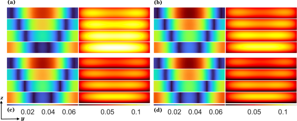
Figure 2: (Color online) Each panel exhibits colormaps of the intensity of order parameter $\psi$ (left column), and the increase of temperature $\Delta=T-T_{0}$ (right) in the $x=0$ plane ($yz$ plane): (a) $h_{f}=0.25,\,h_{s}=0.25$; (b) $h_{f}=0.25,\,h_{s}=0.50$; (a) $h_{f}=0.25,\,h_{s}=0.75$; (a) $h_{f}=0.25,\,h_{s}=1.00$; for all panels $J_{a}=0.049J_{GL}$, $T_{0}=0.75T_{c}$, $l_{x}=24\xi(0)$, $l_{y}=16\xi(0)$, $l_{z}=2.4\xi(0)$. For the order parameter, deep blue indicates regions where the order parameter is significantly degraded, implying a substantial suppression of superconductivity. This phenomenon occurs due to the presence of vortex-antivortex pairs penetrating the superconductor, as indicated by the vertical blue stripes. On the other hand, deep red represents areas where superconductivity is less suppressed, suggesting lesser degradation of the order parameter. For the temperature, red corresponds to regions of lower temperature in the superconductor, where as white denotes areas where the temperature is higher, usually associated with the movement of v-av pairs from their nucleation to their annihilation at the center of the superconductor.

In Fig. 2 we present the intensity of the order parameter and the temperature for $h_{f}=0.25$ and four values of the substrate $h_{s}$. Each panel shows that as the strength of the substrate increases (from panel (a) to (d)), there is a tendency for the temperature of the superconductor to decrease. This demonstrates the effectiveness of a robust substrate in dissipating the heat generated by the movement of v-av pairs. The movement of these pairs is a significant source of heat due to the resistance they offer to the electrical current.

The results from the simulations indicate that the choice and implementation of an efficient substrate are key for thermal control in superconductors, particularly under high DC current conditions.

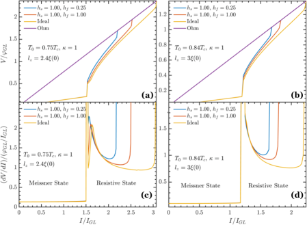
Figure 3: (Color online) IV and IR characteristic curves for $T_{0}=0.75T_{c}$ (panels (a) and (c), respectively) and $T_{0}=0.84T_{c}$ (panels (b) and (d), respectively). Yellow curve represents the results for the simulation which does not solve the heat diffusion equation, while red and blue curves represent results for simulations in which the heat equation is solved with parameters $h_{s}=1.00$, $h_{f}=1.00$ and $h_{s}=1.00$, $h_{f}=0.25$, respectively. The purple curve is the Ohm curve for the voltage at the normal state.

In Fig. 3, we present the characteristic curves for current-voltage (IV) (panels (a) and (b)) and current-resistance (IR) (panels (c) and (d)). These curves correspond to two distinct temperature values: $T_{0}=0.75T_{c}$ (panels (a) and (c)) and $T_{0}=0.84T_{c}$ (panels (b) and (d)). The assigned values for $l_{z}$ are given by $2.4\xi(0)$ and $3\xi(0)$ for $T_{0}=0.75T_{c}$ and $T_{0}=0.84T_{c}$, respectively.

In this figure, the yellow curves illustrate the results when the heat diffusion equation remains unsolved, that is, the temperature is considered homogeneous throughout the superconductor. Hereafter, we refer to this case as the ideal one. In contrast, the remaining two curves incorporate heat dissipation in the simulations. The red curve stands for $h_{s}=1.00$ and $h_{f}=1.00$, which from now on we will denominate by strong heat removal scenario, while the blue curve represents a scenario with a less efficient thermal bath, where $h_{s}=1.00$ and $h_{f}=0.25$.

In all cases, the behavior of the system unfolds as follows. The superconductor initiates from the Meissner state, characterized by the applied current flowing through the stripe in the form of a dissipationless supercurrent. The finite voltage observed in Fig. 3 emerges due to the presence of the normal contacts. Upon reaching a critical current denoted as $I_{c1}$, the superconductor undergoes a transition to the resistive state. In this state, periodic nucleation of v-av pairs occurs at the sample boundaries, followed by their annihilation at the center. As described in Ref. [6], due to the finite thickness of the film, a v-av pair is composed by curved vortex and antivortex which form a closed vortex before annihilating themselves. This dynamics was described in Ref. [6] with an animation presented in the Supplement Material of this reference. As the applied current reaches another critical value, $I_{c2}$, superconductivity is entirely suppressed, leading the superconductor to the normal state.

As can be seen, the transition from the Meissner to the resistive state is unaffected by heat diffusion. The absence of vortices in the Meissner state implies a lack of substantial heat dispersion sources within the system during this phase, thus $I_{c1}$ is the same for all scenarios. In opposition, the value of $I_{c2}$ experiences significant modulation due to the involvement of the heat diffusion equation. Notably, its magnitude is significantly greater when heat considerations are omitted from the simulations. With the inclusion of heat generated by the v-av pairs, the dynamics of the resistive state undergo a clear change. This modification manifests as a reduction in the duration of the resistive state, since the rise in local temperature becomes a contributing factor to the suppression of the superconducting state at lower currents, specially for lower values of $T_{0}$.

The impacts of heat diffusion also manifest in the resistance of the system. Just after $I_{c1}$, the resistance remains nearly unchanged regardless of whether the heat diffusion equation is taken into account or not. However, a distinct shift occurs when currents approach the vicinity of $I_{c2}$, where scenarios involving heat dissipation exhibit higher resistance values. The heat dissipation originating from v-av pairs annihilation rises proportionally with the applied current, rendering the heat diffusion equation progressively more significant within these regions. Consequently, as heat depletes the superconducting state near the critical current $I_{c2}$, the overall medium becomes less conductive to the smooth flow of superconducting current. This accounts for the observed increase in resistance in these situations.

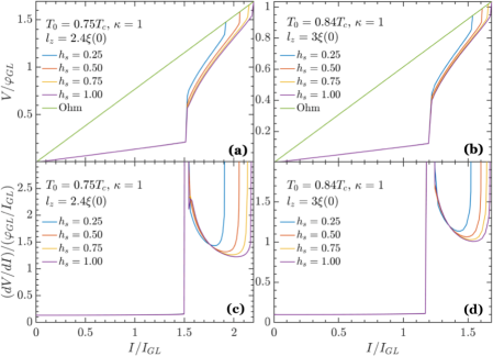
Figure 4: (Color online) IV and IR curves for $T_{0}=0.75T_{c}$ (panels (a) and (c), respectively) and $T_{0}=0.84T_{c}$ (panels (b) and (d), respectively). Each curve represents the results for a different value of $h_{s}$, as specified in the legends. Green curve is the Ohm curve for the voltage at the normal state.

3.2 Efficiency of the Substrate

Having established the importance of accounting for heat diffusion to accurately describe the resistive state, we now examine how the heat removal process influences the behavior of the system. For this purpose, we varied the parameter $h_{s}$, maintaining $h_{f}=0.25$ fixed. In other words, we change the efficiency of heat removal from the superconductor from weak to strong.

In Fig. 4, we present the IV and IR curves for two distinct temperatures ($T_{0}=0.75T_{c}$ and $T_{0}=0.84T_{c}$) and for four different values of $h_{s}$. As described in the preceding Section, the heat produced by the v-av pairs plays a significant role in the reduction of superconductivity, and thus increasing the resistance. This phenomenon is illustrated in panels $(c)$ and $(d)$ of Fig. 4, where the resistance becomes lower near the critical current $I_{c2}$ as the efficiency of heat removal from the sample improves.

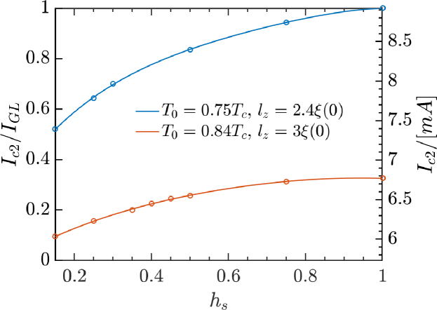
Figure 5: (Color online) Critical current $I_{c2}$ as a function of $h_{s}$ for $T_{0}=0.75T_{c}$ (blue curve) and $T_{0}=0.84T_{c}$ (red curve). Left $y$ axis shows the critical current in dimensionless units, while the right $y$ axis shows the current in real units, using Nb parameters $\xi(0)=39nm$ and $\lambda(0)=50nm$ as a reference.

As anticipated, the efficiency of heat removal also directly impacts the critical current for the transition to the normal state. To facilitate the visualization of the dependence of $I_{c2}$ on the heat removal, Fig. 5 shows $I_{c2}$ as a function of $h_{s}$ for both temperature values. As can be seen, the critical current exhibits a monotonic rise with increasing $h_{s}$, although this variation is not linear. Instead, the change in $I_{c2}$ becomes particularly pronounced for smaller values of $h_{s}$, whereas the critical current presents a gradual increase as we approach a scenario characterized by strong heat removal conditions. To give an idea of what this critical current variation means in a real system, the right $y$ axis presents $I_{c2}$ in real units, with Nb parameters $\xi(0)=39$ nm and $\lambda(0)=50$ nm serving as a reference [20]. The value of $\kappa$ for this material is close to the one used in our simulations. However, we note that, since the parameters used in the heat diffusion equation are general and may not representative of a Nb film. As such values should be considered solely as an estimate of how $I_{c2}$ depends on the substrate efficiency.

By comparing the two curves, a clear distinction emerges, that is, the change in $I_{c2}$ is more pronounced for $T_{0}=0.75T_{c}$. This difference can be attributed to the greater heat dissipation originating from the v-av pairs in this particular scenario. Consequently, the efficiency of the heat removal process becomes more important for the evolution of the superconducting state.

To show that the dissipated heat indeed increases with decreasing system temperature, Fig.6 provides a depiction of the heat transfer rate for all cases illustrated in Fig.4. As it can be seen, at $T_{0}=0.75T_{c}$, the heat extracted from the superconductor surpasses that at $T_{0}=0.84T_{c}$ by a factor of more than two. This difference can be attributed to the nature of the superconducting medium, which becomes increasingly resistant to the passage of a vortex as the superconductivity grows more robust at $T_{0}=0.75T_{c}$, thus leading to a larger dissipated heat. Furthermore, Fig. 6 shows that the heat transfer increases with $h_{s}$, as expected from the previous analysis.

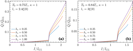
Figure 6: (Color online) Rate of heat transfer as a function of the applied current for $T_{0}=0.75T_{c}$ (panel (a)) and $T_{0}=0.84T_{c}$ (panel (b)). Each curve represents the results for a different value of $h_{s}$, as specified in the legends.

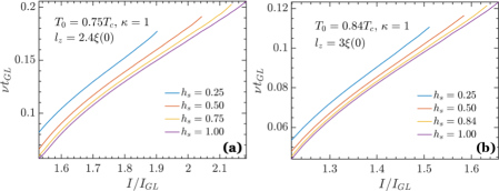
Figure 7: (Color online) Average frequency of the process of creation and annihilation of v-av pairs as a function of the applied current. Panel $(a)$ shows the result for $T_{0}=0.75T_{c}$ and panel $(b)$ for $T_{0}=0.84T_{c}$. Each curve represents a different $h_{s}$, as described in the legends.

To explore the influence of heat removal efficiency on the process of v-av pair creation and annihilation, Fig. 7 presents the frequency of this phenomenon as a function of the applied current. This is demonstrated for different values of $h_{s}$ and two distinct temperatures, namely, $T_{0}=0.75T_{c}$ and $T_{0}=0.84T_{c}$. It becomes clear that, for a given temperature, the frequency of the vortex pair dynamics rises as heat removal from the superconductor becomes less effective. This can be attributed to the decreased viscosity of suppressed superconductivity regions in regard to the motion of vortices. For lower $h_{s}$, a significant proportion of the dissipated heat remains within the superconductor. This heat accumulation increases the local temperature, amplifying the velocity of the v-av pairs. In addition, the authors of Ref. [21] argue that the relaxation time of the order parameter depends on the temperature as $\tau_{|\psi|}=1/(T_{c}-T_{0})$. Indeed, as depicted in Fig. 7, the frequency of v-av pair collisions rises with decreasing $T_{0}$. Consequently, resistance is expected to be greater at lower temperatures. This tendency is clearly observed in panels $(c)$ and $(d)$ of Fig.  3, even in the ideal scenario. This suggests that the observed effect cannot be solely attributed to heat diffusion.

3.3 Effect of the Film Thickness

We now investigate how the thickness of the film influences the characteristics of the resistive state. While keeping the previously defined $l_{x}$ and $l_{y}$ values, we adjust $l_{z}$ to be $4.8\xi(0)$ for $T_{0}=0.75T_{c}$ and $6\xi(0)$ for $T_{0}=0.84T_{c}$. This is depicted in Figs. 8, 9, and 10, which respectively show the IV and IR curves, the heat transfer rate, and the frequency of the creation and annihilation process of v-av pairs as functions of the applied current.

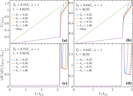
Figure 8: (Color online) IV and IR curves for $T_{0}=0.75T_{c}$, $l_{z}=4.8\xi(0)$ (panels (a) and (c), respectively) and $T_{0}=0.84T_{c}$, $l_{z}=6.0\xi(0)$ (panels (b) and (d), respectively). Each curve represents the results for a different value of $h_{s}$, as specified in the legends. Green curve is the Ohm curve for the voltage at the normal state.

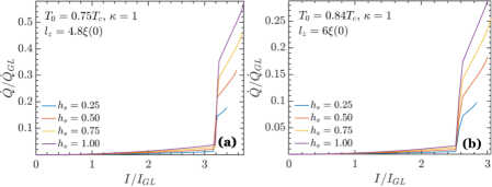
Figure 9: (Color online) Rate of heat transfer as a function of the applied current for $T_{0}=0.75T_{c}$, $l_{z}=4.8\xi(0)$ (panel (a)) and $T_{0}=0.84T_{c}$, $l_{z}=6.0\xi(0)$ (panel (b)). Each curve represents the results for a different value of $h_{s}$, as specified in the legends.

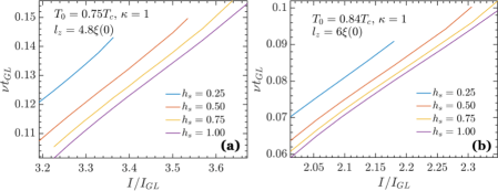
Figure 10: (Color online) Average frequency of the process of creation and annihilation of v-av pairs as a function of the applied current. Panel $(a)$ shows the result for $T_{0}=0.75T_{c}$, $l_{z}=4.8\xi(0)$ and panel $(b)$ for $T_{0}=0.84T_{c}$, $l_{z}=6.0\xi(0)$. Each curve represents a different $h_{s}$, as described in the legends.

These figures show that the system characteristics described in the preceding Section remain unchanged, despite doubling the thickness of the superconductor. However, the figures reveal a new feature, namely that the parameter $h_{s}$ is more important for the quantitative properties of the system. This observation is particularly pronounced for smaller values of $h_{s}$, where heat is less effective and the dissipated heat becomes more important to the evolution of the superconducting state.

This effect stems from two factors. Firstly, by comparing Figs. 6 and 9, we can see that the heat dissipated by the vortex motion is larger for thicker films. Once the superconducting medium is viscous to the vortex flux flow, a larger thickness yields a larger rate of heat transfer. Secondly, a larger thickness means it is more difficult for the heat to be removed from the superconductor by the top and bottom surfaces, thus increasing the importance of the value of $h_{s}$. In addition, the extension of the resistive state, relatively to the Meissner state, is much less than for the thinner superconducting films.

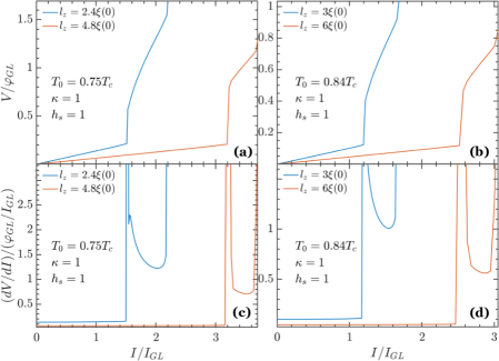
Figure 11: (Color online) IV and IR curves for $T_{0}=0.75T_{c}$ with $l_{z}=2.4\xi(0)$ and $4.8\xi(0)$ (panels (a) and (c), respectively) and $T_{0}=0.84T_{c}$ with $l_{z}=3.0\xi(0)$ and $6.0\xi(0)$ (panels (b) and (d), respectively). In all cases, we have set $h_{s}=1.00$.

To facilitate a detailed comparison between the different thicknesses, Fig. 11 presents the IV and IR curves for $h_{s}=1.00$ of the two simulated thickness values for each temperature. The disparity between $I_{c1}$ and $I_{c2}$ for different thicknesses occurs because the transitions to the resistive and to the normal state are governed by the applied current density $J_{a}$, and their critical values are approximately the same for both films. The second feature that comes apparent in this figure is the difference in the resistance between the thicknesses, with the thicker films displaying a smaller resistance. Although thicker films dissipate more heat, they also carry a larger amount of current, which gives origin to a smaller resistance.

3.4 Hysteresis Loops

After investigating the behavior of the resistive state for various heat removal scenarios and different superconductor thicknesses under increasing applied currents, we now turn our attention to its response as the current is gradually reduced.

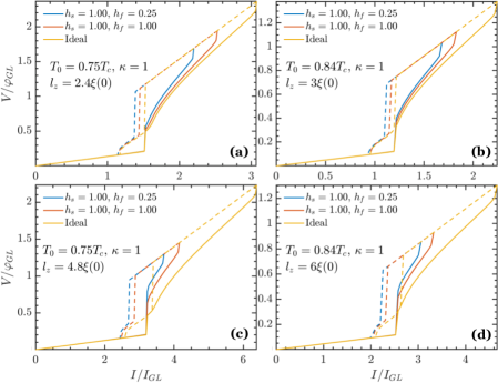
Figure 12: (Color online) IV curves for the upward (solid lines) and downward (dashed lines) sweep directions of the applied current. Panel $(a)$ corresponds to $T_{0}=0.75T_{c}$, $l_{z}=2.4\xi(0)$; panel $(b)$ to $T_{0}=0.84T_{c}$, $l_{z}=3.0\xi(0)$; panel $(c)$ to $T_{0}=0.75T_{c}$, $l_{z}=4.8\xi(0)$; panel $(d)$ to $T_{0}=0.84T_{c}$, $l_{z}=6.0\xi(0)$. Each panel shows the IV curve for the case where the heat diffusion equation is not solved (yellow line), for an strong heat removal scenario with $h_{s}=1.00$, $h_{f}=1.00$ (red line) and for $h_{s}=1.00$ and $h_{f}=0.25.$ (blue line).

In Fig. 12, the IV curves for three distinct systems are displayed. For each system, computed voltage values are presented for both directions of current sweep, encompassing three distinct heat removal scenarios. The first scenario involves the absence of numerical solution for the heat diffusion equation (yellow curve), while the subsequent two scenarios incorporate heat considerations. These include the strong scenario with $h_{f}=1.00$ and $h_{s}=1.00$ (red curve), as well as the scenario with $h_{f}=0.25$ and $h_{s}=1.00$ (blue curve).

Panels $(a)$ and $(b)$ of Fig. 12 illustrate the hysteresis loops for two distinct temperatures: $T_{0}=0.75T_{c}$, with $l_{z}=2.4\xi(0)$, and $T_{0}=0.84T_{c}$, with $l_{z}=3\xi(0)$. Notably, as observed from the yellow curves, in the absence of the heat diffusion equation, the system goes from the normal state back to the resistive state at a critical current $I_{c2}^{*}$ that closely aligns with $I_{c1}$. Below this critical current, the system remains in the resistive state until it reaches $I_{c1}^{*}$, marking the point where it reverts to the Meissner state.

In contrast, for the red and blue curves where the heat diffusion equation is resolved, we can see that the value of $I_{c2}^{*}$ is lower. This discrepancy arises due to the interaction between the recovering superconducting state and the heat generated by the moving vortices. This heat avoids the stabilization of the superconducting state, consequently leading to a reduction in the critical current necessary for the onset of the resistive state.

Furthermore, it is worth noting that the distinction in $I_{c2}^{*}$ between the two cases considering heat and the case where the heat diffusion equation is neglected increases with the thickness of the superconductor. The difference between $I_{c2}^{*}$ of the two cases where heat is taken into account and of the case where the heat diffusion equation is not solved increases with the thickness of the superconductor (compare panels $(a)$ and $(b)$ with panels $(c)$ and $(d)$, respectively). As discussed in the last Section these results reinforce the fact that the diffusion equation becomes more important for thicker films, once the dissipated heat is larger while heat removal also becomes less efficient.

On the other hand, it is noticeable that $I_{c1}^{*}$ is also diminished for the two systems where the heat diffusion equation is accounted for. In these scenarios, the heat generated by the vortices serves to reduce the energy barrier that the v-av pairs must overcome to penetrate the superconductor. This implies the presence of the resistive state at lower current values. Similarly, the system characterized by $h_{f}=0.25$ exhibits a smaller $I_{c1}^{*}$ compared to the system with $h_{f}=1.00$, as the latter benefits from a more efficient heat removal mechanism.

3.5 Effect of the Ginzburg-Landau Parameter

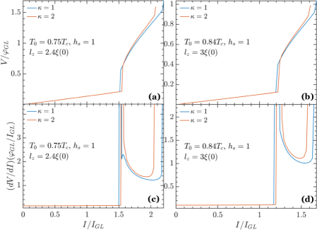
Figure 13: (Color online) IV and IR curves for $\kappa=1.0$ and $2.0$. Panels $(a)$ and $(c)$ corresponds to $T_{0}=0.75T_{c}$ and $l_{z}=2.4\xi(0)$, while panels $(b)$ and $(d)$ corresponds to $T_{0}=0.84T_{c}$ and $l_{z}=3.0\xi(0)$. In all cases, we have set $h_{s}=1.00$.

In Fig. 13, a comparison between the IV and IR curves is presented for two different values of the Ginzburg-Landau parameter, $\kappa=1$ and $\kappa=2$. Despite the similarity in the critical current $I_{c1}$ that marks the beginning of the resistive state for both $\kappa$ values, we can see that $I_{c2}$ decreases and the resistance increases as we increase $\kappa$.

As depicted in Fig.14, a larger $\kappa$ value corresponds to an increased frequency in the process of creating and annihilating v-av pairs. Once a higher frequency also means a larger amount of dissipated heat, we can see that this feature is the responsible for the larger resistance and smaller $I_{c2}$ displayed in Fig.13. The relationship between these quantities is further confirmed by noticing that when the frequency for the two values of $\kappa$ are approximately the same for applied currents near $I_{c1}$, the calculated voltage is also almost equal for both cases. On the other hand, as the applied current approaches $I_{c2}$, the frequency for $\kappa=2$ increases at a larger rate than its counterpart for $\kappa=1$, which is followed by a larger voltage for the former case.

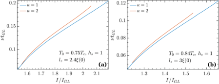
Figure 14: (Color online) Average frequency of the process of creation and annihilation of v-av pairs as a function of the applied current. Panel $(a)$ shows the result for $T_{0}=0.75T_{c}$, $l_{z}=2.4\xi(0)$ and panel $(b)$ for $T_{0}=0.84T_{c}$, $l_{z}=3.0\xi(0)$. In each panel, the blue and the red curves represent $\kappa=1.0$ and $\kappa=2.0$, respectively.

3.6 Comparison with the $2D$ model

Finally, let us investigate the importance of the three-dimensional nature of the method developed here. In other words, we will study how the predictions of our model differ from the ones obtained by the conventional two-dimensional model, very often applied in the literature. In the $2D$ case, Eqs. 1, 2 and 6 are solved in their two-dimensional form, while Eq. 7 is replaced by [10]:

$$\mathcal{C}\frac{\partial T}{\partial t}=\zeta\nabla^{2}T-\eta(T-T_{0})+W,$$ (16)

here, the second term, absent in our $3D$ model, mimics the heat removal from the superconductor by the substrate. As boundary conditions, the temperature is set to be equal to the bath temperature $T_{0}$ in all edges. As defined in Ref. [10], we set $\eta=0.002$, which corresponds to a strong heat removal.

In Fig. 15, we show the IV curves for the $2D$ (blue curve) and $3D$ (red curve) models. The thickness of the superconducting film is $l_{z}=1.0\xi(0)$ and the bath temperature $T=0.84T_{c}$. As one can see, the quantitative difference between the results given by each method is clear. Both critical currents are significantly altered, as the resistive state begins at a much smaller current in the $2D$ case and $J_{c2}$ varies even more, giving rise to a small resistive state range of currents.

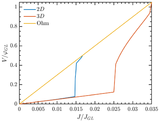
Figure 15: (Color online) Comparison of the IV characteristics obtained with the $2D$ (blue curve) and $3D$ (red curve) models. In the $3D$ model, we have $T=0.84T_{c}$, $l_{z}=1.0\xi(0)$ and $h_{s}=h_{f}=1.00$, while in the $2D$ model, we have $\eta=0.002$.

It is important to note the thickness of the $3D$ film is smaller than the coherence length of the system at the bath temperature, which is usually the condition used to justify the use of $2D$ equations. As shown in Fig. 15, though, while the $2D$ model remains valid to investigate the qualitative behavior of the vortex dynamics in the resistive state of superconducting films, its quantitative predictions fall short when compared to our more complete $3D$ model. This has important consequences to the design of novel superconducting devices, where the precise knowledge of the critical properties of the system under investigation is needed, thus making it necessary the utilization of the $3D$ model.

4 Concluding Remarks

In conclusion, this study highlights the importance of considering the effects of heat diffusion, heat removal efficiency, film thickness, and the Ginzburg-Landau parameter when analyzing the resistive state in superconducting films. These findings contribute to a better understanding of the behavior of superconducting materials under a variety of conditions and offer insights that could have practical implications for the design and applications of superconducting devices, especially regarding the critical parameters. As we have shown, the three-dimensional model used here is of great importance to the precise determination of such quantities, once critical currents obtained within a two-dimensional framework are underestimated.

Acknowledgements

LRC, LVT, and ES thank the Brazilian Agency FAPESP for financial support, grant numbers 20/03947-2, 19/24618-0, 20/10058-0, respectively.

References

- [1] G. Berdiyorov, M. Milošević, F. Peeters, Kinematic vortex-antivortex lines in strongly driven superconducting stripes, Physical Review B 79 (18) (2009) 184506.
- [2] G. Berdiyorov, K. Harrabi, F. Oktasendra, K. Gasmi, A. Mansour, J. Maneval, F. Peeters, Dynamics of current-driven phase-slip centers in superconducting strips, Physical Review B 90 (5) (2014) 054506.
- [3] A. Andronov, I. Gordion, V. Kurin, I. Nefedov, I. Shereshevsky, Kinematic vortices and phase slip lines in the dynamics of the resistive state of narrow superconductive thin film channels, Physica C-superconductivity and Its Applications 213 (1993) 193–199.
-
[4]
A. G. Sivakov, A. M. Glukhov, A. N. Omelyanchouk, Y. Koval, P. Müller, A. V. Ustinov, Josephson behavior of phase-slip lines in wide superconducting strips, Phys. Rev. Lett. 91 (2003) 267001.
doi:10.1103/PhysRevLett.91.267001.
URL https://link.aps.org/doi/10.1103/PhysRevLett.91.267001 - [5] L. R. Cadorim, A. de Oliveira Junior, E. Sardella, Ultra-fast kinematic vortices in mesoscopic superconductors: the effect of the self-field, Scientific Reports 10 (1) (2020) 1–8.
-
[6]
L. R. Cadorim, L. V. de Toledo, W. A. Ortiz, J. Berger, E. Sardella, Closed vortex state in three-dimensional mesoscopic superconducting films under an applied transport current, Phys. Rev. B 107 (2023) 094515.
doi:10.1103/PhysRevB.107.094515.
URL https://link.aps.org/doi/10.1103/PhysRevB.107.094515 - [7] D. Y. Vodolazov, F. Peeters, Rearrangement of the vortex lattice due to instabilities of vortex flow, Physical Review B 76 (1) (2007) 014521.
- [8] A. Presotto, E. Sardella, A. L. Malvezzi, R. Zadorosny, Dynamical regimes of kinematic vortices in the resistive state of a mesoscopic superconducting bridge, Journal of Physics: Condensed Matter 32 (43) (2020) 435702.
- [9] Y.-Y. Lyu, J. Jiang, Y.-L. Wang, Z.-L. Xiao, S. Dong, Q.-H. Chen, M. V. Milošević, H. Wang, R. Divan, J. E. Pearson, et al., Superconducting diode effect via conformal-mapped nanoholes, Nature communications 12 (1) (2021) 2703.
-
[10]
D. Y. Vodolazov, F. M. Peeters, M. Morelle, V. V. Moshchalkov, Masking effect of heat dissipation on the current-voltage characteristics of a mesoscopic superconducting sample with leads, Phys. Rev. B 71 (2005) 184502.
doi:10.1103/PhysRevB.71.184502.
URL https://link.aps.org/doi/10.1103/PhysRevB.71.184502 - [11] C. Aguirre, T. Nunez, J. Barba-Ortega, Vortex matter in heterothermal superconducting loops, Journal of Superconductivity and Novel Magnetism 34 (4) (2021) 1091–1099.
- [12] L. Kramer, R. Watts-Tobin, Theory of dissipative current-carrying states in superconducting filaments, Physical Review Letters 40 (15) (1978) 1041.
- [13] R. Watts-Tobin, Y. Krähenbühl, L. Kramer, Nonequilibrium theory of dirty, current-carrying superconductors: Phase-slip oscillators in narrow filaments near , Journal of Low Temperature Physics 42 (5) (1981) 459–501.
- [14] E. Duarte, E. Sardella, W. Ortiz, R. Zadorosny, Dynamics and heat diffusion of abrikosov’s vortex-antivortex pairs during an annihilation process, Journal of Physics: Condensed Matter 29 (40) (2017) 405605.
- [15] E. Duarte, E. Sardella, T. Saraiva, A. Vasenko, R. Zadorosny, Comparing energy dissipation mechanisms within the vortex dynamics of gap and gapless nano-sized superconductors, Materials Science and Engineering: B 296 (2023) 116656.
- [16] Z. Jing, H. Yong, Y. Zhou, Thermal coupling effect on the vortex dynamics of superconducting thin films: time-dependent ginzburg–landau simulations, Superconductor Science and Technology 31 (5) (2018) 055007.
- [17] A. Schmid, A time dependent ginzburg-landau equation and its application to the problem of resistivity in the mixed state, Physik der kondensierten Materie 5 (4) (1966) 302–317.
- [18] W. D. Gropp, H. G. Kaper, G. K. Leaf, D. M. Levine, M. Palumbo, V. M. Vinokur, Numerical simulation of vortex dynamics in type-II superconductors, Journal of Computational Physics 123 (2) (1996) 254–266.
- [19] L. R. Cadorim, T. de Oliveira Calsolari, R. Zadorosny, E. Sardella, Crossover from type i to type ii regime of mesoscopic superconductors of the first group, Journal of Physics: Condensed Matter 32 (9) (2019) 095304.
- [20] C. P. Poole, H. A. Farach, R. J. Creswick, R. Prozorov, Superconductivity, Elsevier, 2014.
-
[21]
D. Y. Vodolazov, F. M. Peeters, Rearrangement of the vortex lattice due to instabilities of vortex flow, Phys. Rev. B 76 (2007) 014521.
doi:10.1103/PhysRevB.76.014521.
URL https://link.aps.org/doi/10.1103/PhysRevB.76.014521