Nikhef-2024-008

SI-HEP-2024-10

P3H-24-027

Targeting (Pseudo)-Scalar CP Violation with $B_{s}\to\mu^{+}\mu^{-}$

Robert Fleischer ^a,b, Eleftheria Malami ^a,c, Anders Rehult ^a,b, and K. Keri Vos ^a,d

^aNikhef, Science Park 105, NL-1098 XG Amsterdam, Netherlands

^bDepartment of Physics and Astronomy, Vrije Universiteit Amsterdam,
NL-1081 HV Amsterdam, Netherlands

^cCenter for Particle Physics Siegen (CPPS), Theoretische Physik 1,
Universität Siegen, D-57068 Siegen, Germany

^dGravitational Waves and Fundamental Physics (GWFP),
Maastricht University, Duboisdomein 30,
NL-6229 GT Maastricht, the Netherlands

The leptonic decay $B_{s}\to\mu^{+}\mu^{-}$ is both rare and theoretically clean, making it an excellent probe for New Physics searches. Due to its helicity suppression in the Standard Model, this decay is particularly sensitive to new (pseudo)-scalar contributions. We present a new strategy for detecting CP-violating New Physics contributions of this kind, exploiting two observables: $\mathcal{A}_{\Delta\Gamma_{s}}^{\mu\mu}$, which is accessible due to the sizeable decay width difference of the $B_{s}$ system, and the mixing-induced CP asymmetry $\mathcal{S}_{\mu\mu}$. We also utilize information from semileptonic $b\to s\mu^{+}\mu^{-}$ decays. Using the currently available experimental information, we find remarkably constrained regions in the $\mathcal{A}_{\Delta\Gamma_{s}}^{\mu\mu}$–$\mathcal{S}_{\mu\mu}$ plane that serve as promising targets for future measurements.

May 2024

1 Introduction

The leptonic decay $B_{s}\to\mu^{+}\mu^{-}$ is exceptionally rare – out of every billion $B_{s}$ mesons produced, only about three decay into the $\mu^{+}\mu^{-}$ final state [1]. This rarity has made the decay an elusive target. First constraints on its branching ratio were obtained at the Tevatron by the CDF [2] and DØ [3] collaborations, followed by an observation at the LHC, in a joint effort by LHCb and CMS [4]. Recent measurements by LHCb [5], CMS [6], and ATLAS [7] have pushed the experimental precision on the branching ratio to the ten-percent level, a precision set to improve even further in the coming decade [8]. Pioneering analyses have also been performed by LHCb [5], CMS [9], and ATLAS [10] on the $B^{0}_{s}\to\mu^{+}\mu^{-}$ effective lifetime $\tau_{s}^{\mu\mu}$, measurable due to the sizeable decay width difference $\Delta\Gamma_{s}$ of the $B_{s}$ system [11]. The effective lifetime can be converted into the observable $\mathcal{A}_{\Delta\Gamma_{s}}^{\mu\mu}$.

In the Standard Model (SM), the decay is a flavor-changing neutral current process and is helicity suppressed: its branching ratio is proportional to the muon mass squared. Possible new axial-vector, scalar and pseudo-scalar leptonic currents would affect this decay, where the (pseudo)-scalar interactions would lift the helicity suppression. The rarity of the $B_{s}\to\mu^{+}\mu^{-}$ decay thus makes it an excellent choice for indirect New Physics (NP) searches.

In these explorations, both the branching ratio and $\mathcal{A}_{\Delta\Gamma_{s}}^{\mu\mu}$ are important observables, and further data on them are highly valuable. However, $B_{s}\to\mu^{+}\mu^{-}$ has even more information to offer. Theoretical work has identified the mixing-induced CP asymmetry $\mathcal{S}_{\mu\mu}$ as a promising target of study [12, 13]. This observable, accessible through a time-dependent, flavour-tagged analysis, is generated through interference between $\bar{B}^{0}_{s}\to\mu^{+}\mu^{-}$ and $B^{0}_{s}\to\mu^{+}\mu^{-}$ decay processes that originates from $B^{0}_{s}$–$\bar{B}^{0}_{s}$ mixing.

In this paper, we explore new ways to probe possible (pseudo)-scalar contributions by fully exploiting the rare $B_{s}\to\mu^{+}\mu^{-}$ decay. To accomplish this, we need input on possible NP axial-vector interactions. If present, such contributions as well as new (pseudo)-scalar terms would also enter semileptonic rare $b\to s$ transitions. We demonstrate that (pseudo)-scalar interactions are very suppressed in the semileptonic rare $B$-meson decays, thereby allowing us to use these decays to determine the axial-vector NP contributions. This information can then be used to focus the analysis of $B_{s}\to\mu^{+}\mu^{-}$ on (pseudo)-scalar effects.

To achieve this, we present a new strategy to determine whether such possible (pseudo)-scalar NP terms violate CP symmetry. This method exploits the complementary dependence of $\mathcal{A}_{\Delta\Gamma_{s}}^{\mu\mu}$ and $\mathcal{S}_{\mu\mu}$ on such NP effects. In the case of CP-conserving (pseudo)-scalar NP, these observables are strongly correlated: we identify remarkably constrained regions in the $\mathcal{A}_{\Delta\Gamma_{s}}^{\mu\mu}$–$\mathcal{S}_{\mu\mu}$ plane that serve as interesting target regions for future measurements. Any future measurement of these observables outside this target region would indicate CP-violating phases in the (pseudo)-scalar interactions.

This paper is structured as follows: In Sec. 2, we introduce our theoretical framework for $B_{s}\to\mu^{+}\mu^{-}$, construct the relevant observables, and provide SM predictions. We focus in particular on CKM uncertainties. In Sec. 3, we demonstrate how rare semileptonic $B_{(s)}$ decays can be used to determine the axial-vector NP contribution. In Sec. 4, we consider (pseudo)-scalar NP coefficients and show how we obtain our target regions for the $\mathcal{A}_{\Delta\Gamma_{s}}^{\mu\mu}$ and $\mathcal{S}_{\mu\mu}$ observables. We conclude and give a brief outlook in Sec. 5.

2 Theoretical Framework for the $\bar{B}^{0}_{s}\to\mu^{+}\mu^{-}$ Decay

2.1 Effective Hamiltonian

In order to describe the $\bar{B}^{0}_{s}\to\mu^{+}\mu^{-}$ decay, we apply effective quantum field theory, in where heavy SM and NP degrees of freedom are “integrated out”, leading to a low-energy effective Hamiltonian of the following form [14, 11, 15, 12]:

$$\mathcal{H}_{\rm eff}=-\frac{G_{\rm F}}{\sqrt{2}\pi}V_{ts}^{*}V_{tb}\alpha_{\rm em}\left[C_{10}O_{10}+C_{S}O_{S}+C_{P}O_{P}+C_{10}^{\prime}O_{10}^{\prime}+C_{S}^{\prime}O_{S}^{\prime}+C_{P}^{\prime}O_{P}^{\prime}\right]\ .$$ (1)

Here, $G_{\rm F}$ is the Fermi constant, $V_{tb}$ and $V_{ts}^{*}$ are elements of the Cabibbo–Kobayashi–Maskawa (CKM) matrix, and $\alpha_{\rm em}$ is the QED fine structure constant. The four-fermion operators are given as follows:

$$O_{10} =(\bar{s}\gamma_{\mu}P_{L}b)(\bar{\mu}\gamma^{\mu}\gamma_{5}\mu)\ , O_{10}^{\prime} =(\bar{s}\gamma_{\mu}P_{R}b)(\bar{\mu}\gamma^{\mu}\gamma_{5}\mu)\ ,$$ (2)

$$O_{S} =m_{b}(\bar{s}P_{R}b)(\bar{\mu}\mu)\ , O_{S}^{\prime} =m_{b}(\bar{s}P_{L}b)(\bar{\mu}\mu)\ ,$$

$$O_{P} =m_{b}(\bar{s}P_{R}b)(\bar{\mu}\gamma_{5}\mu)\ , O_{P}^{\prime} =m_{b}(\bar{s}P_{L}b)(\bar{\mu}\gamma_{5}\mu)\ ,$$

where $m_{b}$ is the bottom-quark mass, and $P_{R(L)}=\frac{1}{2}(1\pm\gamma_{5})$. In general, the Wilson coefficients depend on the flavour of the final-state leptons [13]. In this paper, we consider only decays into two muons and the corresponding coefficients. In the effective Hamiltonian describing the CP-conjugate processes, all CP-violating phases associated with the Wilson coefficients change their signs.

For convenience, we define the combinations

$$\mathcal{C}_{i}^{\pm} \equiv C_{i}\pm C_{i}^{\prime}\ ,\quad i\in\{10,S,P\}\ ,$$ (3)

for the axial-vector, scalar and psuedo-scalar $\mu\bar{\mu}$ currents. In the SM, only the axial-vector operator $O_{10}$ arises, and we introduce

$$C_{10}\equiv C_{10}^{\rm SM}+C_{10}^{\rm NP}\ .$$ (4)

2.2 Observables and Inputs

Let us discuss the observables of $\bar{B}^{0}_{s}\to\mu^{+}\mu^{-}$ in this subsection. We use (1) to calculate the decay amplitude through evaluating the hadronic matrix element between an initial $B^{0}_{s}$ meson and the final $\mu^{+}\mu^{-}$ state. The decay constant $f_{B_{s}}$ encodes all the hadronic physics and is known with impressive precision from Lattice QCD (LQCD) computations. The HFLAG average [17] utilising the results of [18, 19, 20, 21] yields

$$f_{B_{s}}=(230.3\pm 1.3)\;$\mathrm{MeV}$\ .$$ (5)

The branching ratio of this decay channel in the SM can be written as follows [22]:

$${\mathcal{B}}(B_{s}\to\mu^{+}\mu^{-}) =\frac{G_{F}^{2}\absolutevalue{V_{ts}V_{tb}}^{2}\alpha_{\rm em}^{2}m_{B_{s}}f_{B_{s}}^{2}\tau_{B_{s}}}{64\pi^{3}}\sqrt{1-\frac{4m_{\mu}^{2}}{m_{B_{s}}^{2}}}4m_{\mu}^{2}|C_{10}^{\rm SM}|^{2}\bigg{[}\absolutevalue{P}^{2}+\absolutevalue{S}^{2}\bigg{]}\ ,$$ (6)

which is a CP-averaged quantity. Alternatively, we may replace $\alpha_{\rm em}$ by

$$\alpha_{\rm em}=\frac{2G_{\rm F}^{2}m_{W}^{4}\sin^{4}\theta_{\rm W}}{\pi^{2}}\ ,$$ (7)

where $\theta_{\rm W}$ is the Weinberg angle. Numerically, we use $\alpha_{\rm em}=1/132$, and for the Wilson coefficient we use

$$C_{10}^{\rm SM}=-4.194\ ,$$ (8)

obtained in flavio [23] at the scale $\mu=m_{b}$.

The expression in (6), which holds in the presence of interactions from beyond the SM, introduces the quantities [11]

$$P\equiv\frac{C_{10}-C_{10}^{\prime}}{C_{10}^{\rm SM}}+\frac{M_{B_{s}}^{2}}{2m_{\mu}}\left(\frac{m_{b}}{m_{b}+m_{s}}\right)\left(\frac{C_{P}-C_{P}^{\prime}}{C_{10}^{\rm SM}}\right)\equiv\absolutevalue{P}e^{i\varphi_{P}}\ ,$$ (9)

$$S\equiv\sqrt{1-\frac{4m_{\mu}^{2}}{M_{B_{s}}^{2}}}\frac{M_{B_{s}}^{2}}{2m_{\mu}}\left(\frac{m_{b}}{m_{b}+m_{s}}\right)\left(\frac{C_{S}-C_{S}^{\prime}}{C_{10}^{\rm SM}}\right)\equiv\absolutevalue{S}e^{i\varphi_{S}}\ ,$$ (10)

where $\varphi_{P}$ and $\varphi_{S}$ are CP-violating phases, and $m_{s}=0.093$ MeV denotes the mass of the strange quark. In the SM, we have by definition the following values:

$$P_{\rm SM}=1\ ,\quad\quad S_{\rm SM}=0\ .$$ (11)

The branching ratio ${\mathcal{B}}(B_{s}\to\mu^{+}\mu^{-})$ in (6) exhibits helicity suppression, which is reflected by the $m_{\mu}^{2}$ factor. Looking at (9) and (10), we observe that the helicity suppression can be lifted by the $\mathcal{C}_{P}^{(^{\prime})}$ and $\mathcal{C}_{S}^{(^{\prime})}$coefficients, entering with a factor $1/m_{\mu}$.

The expression of (6) defines the “theoretical” branching ratio at $t=0$. However, after this point the meson starts to oscillate into its antiparticle. What is then measured is the time-integrated branching ratio $\overline{\mathcal{B}}(B_{s}\to\mu^{+}\mu^{-})$, which is related to the theoretical one through [11]

$$\mathcal{B}(B_{s}\to\mu^{+}\mu^{-})_{\rm theo}=\left[\frac{1-y_{s}^{2}}{1+\mathcal{A}_{\Delta\Gamma_{s}}y_{s}}\right]\overline{\mathcal{B}}(B_{s}\to\mu^{+}\mu^{-})\ ,$$ (12)

where

$$\mathcal{B}(B_{s}\to\mu^{+}\mu^{-})_{\rm theo}=\frac{1}{2}\bigg{[}\mathcal{B}(\bar{B}^{0}_{s}\to\mu^{+}\mu^{-})+\mathcal{B}(B^{0}_{s}\to\mu^{+}\mu^{-})\bigg{]}$$ (13)

is the CP-averaged (“untagged”) theoretical branching ratio. The parameter [24]

$$y_{s}\equiv\frac{\Gamma_{\rm L}^{(s)}-\Gamma_{\rm H}^{(s)}}{\Gamma_{\rm L}^{(s)}+\Gamma_{\rm H}^{(s)}}=\frac{\Delta\Gamma_{s}}{2\Gamma_{s}}=0.062\pm 0.004$$ (14)

depends on the decay width difference $\Delta\Gamma_{s}$ between the $B_{s}$ mass eigenstates and on the $B_{s}$ lifetime ${\tau_{B_{s}}}=1/\Gamma_{s}$. Due to $\Delta\Gamma_{s}$, we gain access to

$$\mathcal{A}_{\Delta\Gamma_{s}}=\frac{\absolutevalue{P}^{2}\cos(2\varphi_{P}-\phi_{s}^{\rm NP})-\absolutevalue{S}^{2}\cos(2\varphi_{S}-\phi_{s}^{\rm NP})}{\absolutevalue{P}^{2}+\absolutevalue{S}^{2}}\ .$$ (15)

This observable is given by $+1$ in the SM but can generally take any value between $-1$ and $+1$. The phase $\phi_{s}^{\rm NP}$ is related to CP-violating contributions from beyond the SM to $B^{0}_{s}$–$\bar{B}^{0}_{s}$ mixing:

$$\phi_{s}^{\rm NP}=\phi_{s}-\phi_{s}^{\rm SM}\ .$$ (16)

Following [25, 26], we combine the value of $\phi_{s}$ with the SM prediction $\phi_{s}^{\rm SM}$. The $\phi_{s}$ comes from decays of the kind $B^{0}_{s}\to J/\psi\phi$, where contributions from penguin topologies have been taken into account [27]:

$$\phi_{s}=(-4.2\pm 1.4)^{\circ}\ .$$ (17)

The SM value arises from an analysis of the Unitarity Triangle (UT) utilising only information from the angle $\gamma$ and the side $R_{b}$ [27]:

$$\phi_{s}^{\rm SM}=(-2.01\pm 0.12)^{\circ}\ .$$ (18)

Finally, using (19), the NP phase is determined as [27]

$$\phi_{s}^{\rm NP}=(2.2\pm 1.4)^{\circ}\ ,$$ (19)

which is the value we use in order to include NP contributions to $B^{0}_{s}$–$\bar{B}^{0}_{s}$ mixing.

We note that $\mathcal{A}_{\Delta\Gamma_{s}}^{\mu\mu}$ can be obtained from measurements of the $B_{s}\to\mu^{+}\mu^{-}$ effective lifetime, defined as follows (see also [11, 12]):

$$\tau_{\mu\mu}^{s}\equiv\frac{\int_{0}^{\infty}t\langle\Gamma(B_{s}(t)\to\mu^{+}\mu^{-})\rangle dt}{\int\int_{0}^{\infty}\langle\Gamma(B_{s}(t)\to\mu^{+}\mu^{-})\rangle dt}\ .$$ (20)

Measuring this quantity requires time information for untagged data samples. ATLAS [10], CMS [6] and the LHCb Collaboration [5] have all recently reported measurements of the effective lifetime $\tau_{\mu\mu}^{s}$:

$$\tau_{\mu\mu}^{s}|_{\rm LHCb\;2021} =(2.07\pm 0.29)\;$\mathrm{p}\mathrm{s}$\ ,$$ (21)

$$\tau_{\mu\mu}^{s}|_{\rm CMS\;2022} =(1.83\pm 0.23)\;$\mathrm{p}\mathrm{s}$\ ,$$

$$\tau_{\mu\mu}^{s}|_{\rm ATLAS\;2023} =(0.99\pm 0.45)\;$\mathrm{p}\mathrm{s}$\ .$$

Using the following relation [11]:

$$\mathcal{A}_{\Delta\Gamma_{s}}^{\mu\mu}=\frac{1}{y_{s}}\left[\frac{(1-y_{s}^{2})\tau_{\mu\mu}^{s}-(1+y_{s}^{2})\tau_{B_{s}}}{2\tau_{B_{s}}-(1-y_{s}^{2})\tau_{\mu\mu}^{s}}\right]\ ,$$ (22)

the above results can be translated into bounds on $\mathcal{A}_{\Delta\Gamma_{s}}^{\mu\mu}$, yielding:

$$\mathcal{A}_{\Delta\Gamma_{s}}^{\mu\mu}|_{\rm LHCb\;2021} =8.44\pm 7.11\ ,$$ (23)

$$\mathcal{A}_{\Delta\Gamma_{s}}^{\mu\mu}|_{\rm CMS\;2022} =3.75\pm 3.68\ ,$$

$$\mathcal{A}_{\Delta\Gamma_{s}}^{\mu\mu}|_{\rm ATLAS\;2023} =-4.08\pm 2.52\ .$$

Unfortunately, the uncertainties are still too large to constrain the observable within its model-independent range of $-1\leq\mathcal{A}_{\Delta\Gamma_{s}}^{\mu\mu}\leq 1$.

Finally, we can also consider the full time-dependent rate of the $B_{s}$ mesons decaying into two muons with helicity $\lambda=L,R$. Even though the expression in (6) corresponds to a summation over helicities, it is now useful to work on the case for specific helicities. A flavour-tagged analysis would then give access to the CP-violating decay rate asymmetry [11, 22]:

$$\frac{\Gamma(B^{0}_{s}(t)\to\mu_{\lambda}^{+}\mu_{\lambda}^{-})-\Gamma(\bar{B}^{0}_{s}(t)\to\mu_{\lambda}^{+}\mu_{\lambda}^{-})}{\Gamma(B^{0}_{s}(t)\to\mu_{\lambda}^{+}\mu_{\lambda}^{-})+\Gamma(\bar{B}^{0}_{s}(t)\to\mu_{\lambda}^{+}\mu_{\lambda}^{-})}=\frac{\mathcal{C}_{\mu\mu}^{\lambda}\cos(\Delta M_{s}t)+\mathcal{S}_{\mu\mu}\sin(\Delta M_{s}t)}{\cosh(y_{s}t/\tau_{B_{s}})+\mathcal{A}_{\Delta\Gamma_{s}}^{\mu\mu}\sinh(y_{s}t/\tau_{B_{s}})}\ ,$$ (24)

with the CP asymmetries

$$\mathcal{C}_{\mu\mu}^{\lambda}=-\eta_{\lambda}\left[\frac{2\absolutevalue{PS}\cos(\varphi_{P}-\varphi_{S})}{\absolutevalue{P}^{2}+\absolutevalue{S}^{2}}\right]\equiv-\eta_{\lambda}\mathcal{C}_{\mu\mu}\ ,$$ (25)

$$\mathcal{S}_{\mu\mu}=\frac{\absolutevalue{P}^{2}\sin(2\varphi_{P}-\phi_{s}^{\rm NP})-\absolutevalue{S}^{2}\sin(2\varphi_{S}-\phi_{s}^{\rm NP})}{\absolutevalue{P}^{2}+\absolutevalue{S}^{2}}\ ,$$ (26)

both of which are zero in the SM. The observable $\mathcal{C}_{\mu\mu}^{\lambda}$ depends on the helicity of the lepton pair ($\eta_{L}=+1$ and $\eta_{R}=-1$), making it difficult to measure. However, we stress that even knowing its sign would already be useful to resolve discrete ambiguities that arise when determining (pseudo)-scalar Wilson coefficients [12]. We note that no data are yet available for $\mathcal{S}_{\mu\mu}$ and $\mathcal{C}_{\mu\mu}$.

Keeping the time dependence but summing over the muon helicities, (24) becomes

$$\frac{\Gamma(B^{0}_{s}(t)\to\mu^{+}\mu^{-})-\Gamma(\bar{B}^{0}_{s}(t)\to\mu^{+}\mu^{-})}{\Gamma(B^{0}_{s}(t)\to\mu^{+}\mu^{-})+\Gamma(\bar{B}^{0}_{s}(t)\to\mu^{+}\mu^{-})}=\frac{\mathcal{S}_{\mu\mu}\sin(\Delta M_{s}t)}{\cosh(y_{s}t/\tau_{B_{s}})+\mathcal{A}_{\Delta\Gamma_{s}}^{\mu\mu}\sinh(y_{s}t/\tau_{B_{s}})}\ .$$ (27)

The three observables $\mathcal{A}_{\Delta\Gamma_{s}}^{\mu\mu}$, $\mathcal{S}_{\mu\mu}$, and $\mathcal{C}_{\mu\mu}$ are theoretically clean since the decay constant $f_{B_{s}}$ cancels in all of them. They satisfy the relation

$$(\mathcal{A}_{\Delta\Gamma_{s}}^{\mu\mu})^{2}+(\mathcal{S}_{\mu\mu})^{2}+(\mathcal{C}_{\mu\mu})^{2}=1\ ,$$ (28)

and are therefore not independent of one another.

2.3 Information from Branching Ratios

The SM prediction for the branching ratio in (6) depends on the CKM matrix elements entering $|V_{ts}V_{tb}|$. Using the Wolfenstein parametrization, we obtain

$$|V_{ts}V_{tb}|=\phantom{\lambda}|V_{cb}|\left[1-\frac{\lambda^{2}}{2}\left(1-2R_{b}\cos\gamma\right)\right]+\mathcal{O}\left(\lambda^{6}\right)\>,$$ (29)

where $\lambda\equiv|V_{us}|$, the parameter

$$R_{b}\equiv\left|\frac{V_{ud}V_{ub}^{*}}{V_{cd}V_{cb}^{*}}\right|=\left(1-\frac{\lambda^{2}}{2}\right)\frac{1}{\lambda}\left|\frac{V_{ub}}{V_{cb}}\right|\ ,$$ (30)

is the usual side of the UT from the origin to the apex, and $\gamma$ is the corresponding angle. Expression (29) is governed by $|V_{cb}|$ up to $\mathcal{O}({\lambda^{2}})$ corrections, which involve $R_{b}$ and $\gamma$.

To determine $|V_{ts}V_{tb}|$, we thus require values for $|V_{ub}|$ and $|V_{cb}|$. This poses a problem, as these CKM factors carry a substantial, hidden theoretical uncertainty. There are two methods to determine $|V_{ub}|$ and $|V_{cb}|$. One uses exclusive decay processes and the other inclusive measurements. Ideally, both determinations should agree with each other, but in practice, tensions arise. These long-standing tensions constitute the key uncertainty for the branching ratio, and special care is needed. Therefore, we study separately the inclusive and exclusive case, as discussed in [26]. In addition to these two determinations, a hybrid approach combining the exclusive $|V_{ub}|$ with the inclusive $|V_{cb}|$ values was also studied [26].

In the inclusive and hybrid scenarios, the results for $|V_{ts}V_{tb}|$ are the same. Using input from inclusive $b\to c\ell\nu_{\ell}$ decays [28], we obtain:

$$|V_{ts}V_{tb}|_{\rm incl/hybrid}=(41.4\pm 0.5)\times 10^{-3}\ .$$ (31)

Taking the exclusive $|V_{cb}|$ from the HFLAV collaboration [29], we find

$$|V_{ts}V_{tb}|_{\rm excl}=(38.4\pm 0.5)\times 10^{-3},$$ (32)

which differs from (31) at the $4\sigma$ level due to the different $|V_{cb}|$ values. Finally, we find the following predictions for the SM values of the branching ratios:

$$\overline{\mathcal{B}}(B_{s}\to\mu^{+}\mu^{-})_{\rm SM}^{\rm incl/hybrid} =(3.71\pm 0.04|_{f_{B_{s}}}\pm 0.09|_{\rm CKM}\pm 0.02|_{\rm source})\cdot 10^{-9}$$

$$=(3.71\pm 0.10)\cdot 10^{-9}\ ,$$ (33)

$$\overline{\mathcal{B}}(B_{s}\to\mu^{+}\mu^{-})_{\rm SM}^{\rm excl} =(3.19\pm 0.04|_{f_{B_{s}}}\pm 0.08|_{\rm CKM}\pm 0.02|_{\rm source})\cdot 10^{-9}$$

$$=(3.19\pm 0.09)\cdot 10^{-9}\ .$$ (34)

It becomes clear that there is a significant variation depending on the CKM parametrization. Thus, special attention is needed for the CKM uncertainties. The results in (33) and (34) are in the ballpark of other theoretical predictions [30], and we note that the spread between inclusive and exclusive results is much wider than the quoted uncertainties.

The current experimental world average stands at [31]

$$\overline{\mathcal{B}}(B_{s}\to\mu^{+}\mu^{-})=(3.45\pm 0.29)\times 10^{-9}\ ,$$ (35)

relying mainly on recent measurements by LHCb [5], CMS [6], and ATLAS [7]. This experimental average is smaller than the inclusive SM prediction in (33) but larger than the exclusive SM prediction in (34).

Moving now towards studies of NP, we introduce the ratio between the experimental and SM branching ratios:

$$\overline{R}=\frac{\overline{\mathcal{B}}(B_{s}\to\mu^{+}\mu^{-})}{\overline{\mathcal{B}}(B_{s}\to\mu^{+}\mu^{-})_{\rm SM}}\ .$$ (36)

In the SM, by definition $\overline{R}=1$. Combining the current experimental results in (35) with the inclusive/hybrid and exclusive values for the SM predictions in (33) and (34), we obtain

$$\overline{R}_{\rm incl/hybrid} =0.93\pm 0.082\ ,$$ (37)

$$\overline{R}_{\rm excl} =1.08\pm 0.096\ ,$$ (38)

where we see again that the experimental result can be either larger or smaller than the SM prediction, depending on the choice of the CKM parameterization.

Taking into account the difference between the time-integrated and theoretical branching ratios, $\overline{R}$ can be written as follows [22]:

$$\overline{R} =\bigg{[}\frac{1+\mathcal{A}_{\Delta\Gamma_{s}}^{\mu\mu}y_{s}}{1+y_{s}}\bigg{]}(|P|^{2}+|S|^{2})$$

$$=\left[\frac{1+y_{s}\cos(2\varphi_{P}-\phi_{s}^{\rm NP})}{1+y_{s}}\right]|P|^{2}+\left[\frac{1-y_{s}\cos(2\varphi_{S}-\phi_{s}^{\rm NP})}{1+y_{s}}\right]|S|^{2}\ ,$$ (39)

where $S$ and $P$ are given in (10) and (9), respectively. Using the value of $\phi_{s}^{\rm NP}$ in (19) and assuming real (pseudo)-scalar couplings, i.e. $\varphi_{P}=\varphi_{S}=0$, this ratio constrains a circle in the $|P|$–$|S|$ plane. In Fig. 1, we show the circles that result from using the inclusive/hybrid and exclusive values of $\overline{R}$. We note that within their respective uncertainties these circles overlap. The SM point, with $P_{\rm SM}=1$ and $S_{\rm SM}=0$, is also indicated and lies between both predictions. Allowing for physics beyond the SM, entering through $\mathcal{C}^{-}_{10}$ and/or through new (pseudo)-scalar couplings in $\mathcal{C}^{-}_{S,P}$, the branching ratio thus constrains a combination of these possible new couplings. In the following, we discuss how to disentangle these possible NP effects. For our analysis, we will use the incl/hybrid value for the CKM elements.

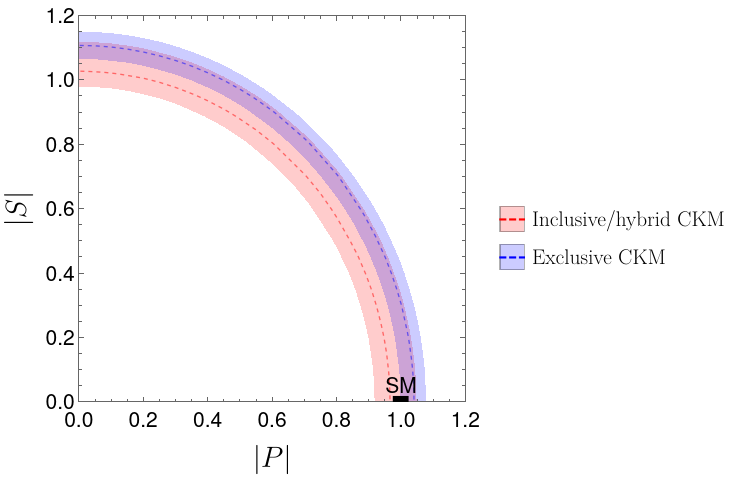
Figure 1: Constraints in the $|P|$–$|S|$ plane from the current world average experimental measurement of $\mathcal{B}(B_{s}\to\mu^{+}\mu^{-})$ for the inclusive/hybrid and exclusive CKM parameterizations.

3 Extracting $\mathcal{C}^{-}_{10}$ from Semileptonic Rare $B_{(s)}$ Decays

The leptonic $B_{s}\to\mu^{+}\mu^{-}$ decay is governed by combinations of the scalar and pseudo-scalar Wilson coefficients. As seen in (9) and (10), $\mathcal{C}^{-}_{P}$ and $\mathcal{C}^{-}_{S}$ enter in $P$ and $S$, respectively. In addition, $P$ contains the coefficient $\mathcal{C}^{-}_{10}$. The quantities $P$ and $S$ can be determined through observables of the $B_{s}\to\mu^{+}\mu^{-}$ channel, as discussed in [13]. However, in order to constrain the corresponding Wilson coefficients, we have to disentangle the $\mathcal{C}^{-}_{10}$ and $\mathcal{C}^{-}_{P}$ contributions which both enter $P$. Fortunately, we can do this by extracting $\mathcal{C}^{-}_{10}$ from semileptonic decays of the kind $B\to K^{(*)}\mu^{+}\mu^{-}$ and $B_{s}\to\phi\mu^{+}\mu^{-}$. Let us now have a closer look at how we can accomplish this task.

3.1 Theoretical Framework

Decay	Wilson Coefficients
$B_{s}\to\phi\mu^{+}\mu^{-}$	$\mathcal{C}^{+}_{9},\mathcal{C}^{-}_{9},\mathcal{C}^{+}_{10},\mathcal{C}^{-}_{10},(\mathcal{C}^{-}_{P},\mathcal{C}^{-}_{S})$
$B\to K^{*}\mu^{+}\mu^{-}$	$\mathcal{C}^{+}_{9},\mathcal{C}^{-}_{9},\mathcal{C}^{+}_{10},\mathcal{C}^{-}_{10},(\mathcal{C}^{-}_{P},\mathcal{C}^{-}_{S})$
$B\to K\mu^{+}\mu^{-}$	$\mathcal{C}^{+}_{9},\mathcal{C}^{+}_{10},(\mathcal{C}^{+}_{P},\mathcal{C}^{+}_{S})$
$B_{s}\to\mu^{+}\mu^{-}$	$\mathcal{C}^{-}_{10},\mathcal{C}^{-}_{P},\mathcal{C}^{-}_{S}$

Table 1: Rare $B$ decays and their dependence on the Wilson coefficients. Parentheses indicate negligible dependencies.

The semileptonic $B_{(s)}\to K^{\ast}(\phi)\mu^{+}\mu^{-}$ and $B\to K\mu^{+}\mu^{-}$ modes are described by the weak Hamiltonian

$$\mathcal{H}_{\rm eff}=-\frac{G_{F}}{\sqrt{2}\pi}V_{ts}^{*}V_{tb}\alpha_{\rm em}\sum\limits_{i\in I}C_{i}\mathcal{O}_{i}\ ,$$ (40)

where we have neglected doubly Cabibbo-suppressed terms. The sum runs over the index $I=\{1c,2c,3,4,5,6,8,7^{(\prime)},9^{(\prime)}\mu,10^{(\prime)}\mu,S^{(\prime)}\mu,P^{(\prime)}\mu,T^{(\prime)}\mu\}$ and includes all operators that can contribute to the modes. In particular, in contrast with $B_{s}\to\mu^{+}\mu^{-}$, now also the following operators enter:

$$\mathcal{O}_{9^{(\prime)}\mu}=[\bar{s}\gamma^{\mu}P_{L(R)}b](\bar{\mu}\gamma_{\mu}\mu)\ ,\quad\mathcal{O}_{7^{(\prime)}}=\frac{1}{e}m_{b}[\bar{s}\sigma^{\mu\nu}P_{R(L)}b]F_{\mu\nu}\ ,$$ (41)

with $\sigma_{\mu\nu}=\frac{i}{2}[\gamma_{\mu},\gamma_{\nu}]$. In the SM, we have [23]

$$C_{9}^{\rm SM}=4.114\ ,\quad\quad C_{7}^{\rm SM}=-0.296\ .$$ (42)

Expressions for the differential rate of the $B_{(s)}\to K^{*}(\phi)\mu^{+}\mu^{-}$ modes are given in e.g., [16], while those for $B\to K\mu^{+}\mu^{-}$ can be found in e.g., [32]. In the following, we neglect NP contributions to $C_{7}$ and the tensor coefficient $C_{T}$. The branching ratios then depend on specific combinations of $C_{9,10,S,P}$, given in Table 1, where we have defined

$$\mathcal{C}_{9}^{\pm}\equiv C_{9}\pm C_{9}^{\prime}$$ (43)

in analogy with (3).

In the $B_{(s)}\to K^{*}(\phi)$ modes, there are several additional observables besides the branching ratio (see, e.g., [16] for an overview). It is important to note that, unlike the $B_{s}\to\mu^{+}\mu^{-}$ channel, the semileptonic modes are not helicity suppressed. As a result, they are much less sensitive than the $B_{s}\to\mu^{+}\mu^{-}$ decay to $C_{P}$ and $C_{S}$.

Recent predictions for the branching ratio of $B\to K\mu^{+}\mu^{-}$ can be found in [32]. For the $B_{s}\to\phi$ and $B\to K^{*}$ modes, we present the SM predictions using the inputs above, the LQCD and Light-cone sum rule (LCSR) form factors from [33] and perturbative long-distance effects from [16]. We find the following SM predictions in the $1.1<~{}q^{2}<~{}6.0\;$\mathrm{G}\mathrm{eV}^{2}$$ range:

$$\overline{\mathcal{B}}(B_{s}\to\phi\mu^{+}\mu^{-})|_{\rm incl/hybrid}{} =(5.63\pm 0.58)\cdot 10^{-8}\ ,$$ (44)

$$\overline{\mathcal{B}}(B_{s}\to\phi\mu^{+}\mu^{-})|_{\rm excl}{} =(4.85\pm 0.49)\cdot 10^{-8}\ .$$ (45)

Analogous to the discussion in Sec. 2.2, we converted the theoretical rate to the experimental branching ratio corresponding to time-integrated untagged data samples following [16]. Again we note the significant difference in the SM predictions depending on the CKM matrix element determinations, which was also noted, e.g., in [32]. For the $K^{*}$ modes, we find

$$\mathcal{B}(B\to K^{*\pm}\mu^{+}\mu^{-})|_{\rm incl/hybrid}{} =(5.35\pm 0.72)\cdot 10^{-8}\ ,$$

$$\mathcal{B}(B\to K^{(*\pm)}\mu^{+}\mu^{-})|_{\rm excl}{} =(4.61\pm 0.61)\cdot 10^{-8}\ ,$$ (46)

and

$$\overline{\mathcal{B}}(B\to K^{*0}\mu^{+}\mu^{-})|_{\rm incl/hybrid}{} =(5.00\pm 0.64)\cdot 10^{-8}\ ,$$

$$\overline{\mathcal{B}}(B\to K^{*0}\mu^{+}\mu^{-})|_{\rm excl}{} =(4.31\pm 0.55)\cdot 10^{-8}\ .$$ (47)

These results agree within uncertainties with [34, 33, 23]. The experimental values measured by the LHCb Collaboration [35, 36] are given as follows:

$$\overline{\mathcal{B}}(B_{s}\to\phi\mu^{+}\mu^{-})|_{\rm exp}=(2.88\pm 0.21)\cdot 10^{-8}\ ,$$ (48)

and

$$\overline{\mathcal{B}}(B^{\pm}\to K^{(*\pm)}\mu^{+}\mu^{-})|_{\rm exp}=(3.66\pm 0.87)\cdot 10^{-8}\ .$$ (49)

We find that the experimental branching ratios are smaller than the SM predictions, a trend that is also reflected in the semileptonic $B\to K\mu^{+}\mu^{-}$ channel (see e.g., [32]). These anomalies are well known and have been the focus of many global fits, see e.g., [37, 38, 39, 40, 41, 34, 42, 43, 44], where usually the coefficient $C_{9}^{(\prime)}$ shows the largest statistical pull away from its SM value. However, NP may well also enter through $C_{10}^{(\prime)}$.

3.2 Extracting $\mathcal{C}^{-}_{10}$

The first step of our analysis is to determine $\mathcal{C}^{-}_{10}$ from the rare semileptonic decays and then $\mathcal{C}^{-}_{P,S}$ from $B_{s}\to\mu^{+}\mu^{-}$. However, $\mathcal{C}^{-}_{P}$ and $\mathcal{C}^{-}_{S}$ also enter the semileptonic modes. We will show that the impact of $\mathcal{C}^{-}_{P,S}$ on the semileptonic decays is actually small, and consequently we can determine $\mathcal{C}^{-}_{10}$ through these decays even though they in principle also depend on $\mathcal{C}^{-}_{P,S}$.

We simplify the analysis by only allowing for real NP coefficients and assuming that no NP enters in $C_{9}^{(\prime)}$. We illustrate in Fig. 2 the current constraint from the branching ratio of $B_{s}\to\mu^{+}\mu^{-}$ in the $\mathcal{C}^{-}_{P}$–$\mathcal{C}^{-}_{S}$ plane. In addition, we show the branching ratio of $B_{s}\to\phi\mu^{+}\mu^{-}$ as a function of $\mathcal{C}^{-}_{P}$ and $\mathcal{C}^{-}_{S}$. The three ellipses represent the SM value in (44) and allowing for a range the SM value $\pm$ 0.5 %, specifically $[5.60,5.66]\times 10^{-8}$. For Fig. 2, we assume $\mathcal{C}_{10}^{-\rm NP}=0$, but we find similar results when $\mathcal{C}_{10}^{-\rm NP}\neq 0$. We observe that the current $B_{s}\to\mu^{+}\mu^{-}$ measurement already constrains $\absolutevalue{\mathcal{C}^{-}_{P,S}}\leq 0.06\;$\mathrm{G}\mathrm{eV}^{-1}$$. On the other hand, we find that a NP contribution of that size affects the semileptonic branching ratio only at the percent level. This demonstrates that the leptonic decay is indeed significantly more sensitive than the semileptonic one to (pseudo)-scalar NP and that $\mathcal{C}^{-}_{P,S}$ can only affect the branching ratio of $B_{s}\to\phi\mu^{+}\mu^{-}$ at the level of less than one percent. We obtain similar results for the $B^{\pm}\to K^{\pm\ast}\mu^{+}\mu^{-}$ and $B^{\pm}\to K^{\pm}\mu^{+}\mu^{-}$ decays.

The small sensitivity of the semileptonic decays with respect to new (pseudo)-scalar contributions can also be seen by looking at the observables $R_{S}$ and $R_{W}$, defined in (66) and (68) of [45]. These are constructed to be sensitive to scalar NP contributions, and $R_{W}$ vanishes for $m_{\ell}=0$ and $\mathcal{C}^{-}_{S}=\mathcal{C}^{-}_{T}=0$. However, as was also noted in [45], $R_{S}$ only changes minimally when allowing for new scalar contributions. In addition, $R_{W}$ does get affected by new scalar couplings, but its value remains of $\mathcal{O}(10^{-2})$. Therefore, only very precise experimental information on these observables, which are currently not measured, might help in constraining $\mathcal{C}^{-}_{P,S}$.

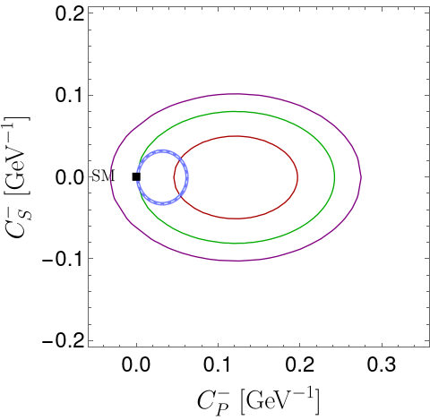
(a)

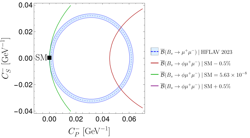
(b)

Figure 2: Correlation between $\mathcal{C}^{-}_{P}$ and $\mathcal{C}^{-}_{S}$ for $\mathcal{C}_{10}^{-\rm NP}=0$. The blue circular band is the $1\sigma$ constraint from $\overline{\mathcal{B}}(B_{s}\to\mu^{+}\mu^{-}$) in (35), and the ellipses indicate values of $\overline{\mathcal{B}}(B_{s}\to\phi\mu^{+}\mu^{-})$ in the $q^{2}\in[1.1,6.0]\;$\mathrm{G}\mathrm{eV}^{2}$$ bin.

We have demonstrated that semileptonic rare $B$ decays are much less sensitive to (pseudo)-scalar NP than the leptonic $B_{s}\to\mu^{+}\mu^{-}$ channel. For this reason, we may neglect $\mathcal{C}^{-}_{P}$ and $\mathcal{C}^{-}_{S}$ and extract $\mathcal{C}^{-}_{10}$ from the rare semileptonic $b\to s$ decays. In Fig. 3 we illustrate the results of such an extraction as contours in the $C_{10}^{\rm NP}$–$C_{10}^{\prime\rm NP}$ plane, assuming (a) $C_{9}^{(\prime)\rm NP}=0$ and (b) $C_{9}^{(\prime)\rm NP}=-C_{10}^{(\prime)\rm NP}$. Here we show constraints from the branching ratios of $B_{s}\to\phi\mu^{+}\mu^{-}$ (blue), $B\to K^{*}\mu^{+}\mu^{-}$ (orange), and $B\to K\mu^{+}\mu^{-}$ (green). The contour following from $B\to K\mu^{+}\mu^{-}$ is a pair of straight diagonal lines because this decay depends only on $\mathcal{C}^{+}_{10}$. The contours from the vector modes, on the other hand, are ellipses, since those decays depend on both $\mathcal{C}^{+}_{10}$ and $\mathcal{C}^{-}_{10}$. By using data on the three branching ratios together, we can determine $C_{10}$ and $C_{10}^{\prime}$ up to a fourfold ambiguity. We mark the resulting four points by card suits and give the corresponding values of $\mathcal{C}^{-}_{10}$ and $\mathcal{C}^{+}_{10}$ in Tab. 2. We note that especially the interplay between $B^{\pm}\to K^{\pm}\mu^{+}\mu^{-}$ and $B_{s}\to\phi\mu^{+}\mu^{-}$ strongly constrains the allowed region for $C_{10}^{(^{\prime})}$, i.e. at the $1\sigma$ level, the size of the symbols basically corresponds to the allowed regions. In the case of CP-violating NP in $\mathcal{C}^{-}_{10}$, the rare semileptonic $B$ decays can also be used to constraint its complex coefficients using CP-asymmetries [32] and possible angular observables for the vector modes.

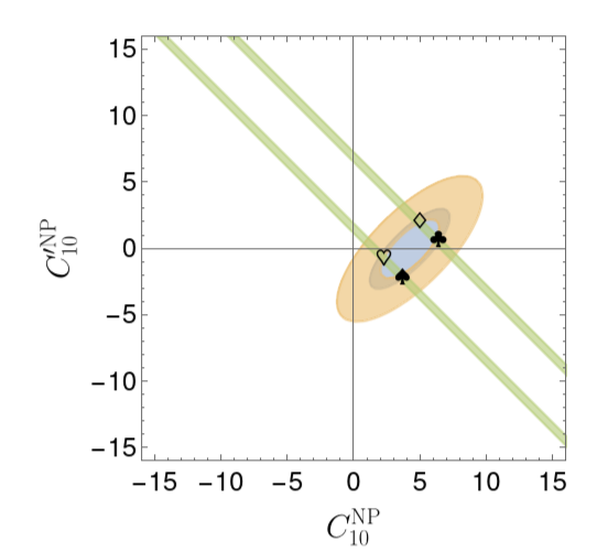
(a)

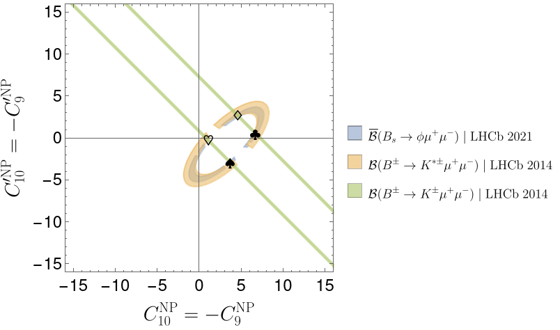
(b)

Figure 3: Bounds on $C_{10}^{\rm NP}$ and $C_{10}^{\prime\rm NP}$ from semileptonic $b\to s\mu^{+}\mu^{-}$ decays, assuming real Wilson coefficients. The four points mark the overlapping region and are given in Table 2.

Symbol	$C_{10}^{\rm NP}$	$C_{10}^{\prime\rm NP}$
$\heartsuit$	$2.3$	$-0.7$
$\spadesuit$	$3.7$	$-2.1$
$\diamondsuit$	$5.0$	$2.1$
$\clubsuit$	$6.4$	$0.7$

Symbol	$C_{10}^{\rm NP}$	$C_{10}^{\prime\rm NP}$
$\heartsuit$	$1.1$	$-0.3$
$\spadesuit$	$3.7$	$-3.0$
$\diamondsuit$	$4.6$	$2.7$
$\clubsuit$	$6.7$	$0.4$

Table 2: Values of $C_{10}^{\rm NP}$ and $C_{10}^{\prime\rm NP}$ at the four marked points in Fig. 3. Left: $C_{9}^{(\prime)\rm NP}=0$. Right: $C_{9}^{(\prime)\rm NP}=-C_{10}^{(\prime)\rm NP}$.

We can compare these constraints with those obtained $B_{s}\to\mu^{+}\mu^{-}$. Assuming no (pseudo)-scalar NP contributions, the experimental data on $\overline{\mathcal{B}}(B_{s}\to\mu^{+}\mu^{-})$ imposes two diagonal lines in the $C_{10}^{\rm NP}$–$C_{10}^{\prime\rm NP}$ plane as shown in Fig. 4, where we have used as our experimental input (35). Due to the precision of the experimental results, there is no overlap at the $1\sigma$-level with the points determined from the semileptonic decays. This suggests that NP contributions only to $C_{10}$ and $C_{10}^{\prime}$, or to $C_{10}^{(\prime)}=-C_{9}^{(\prime)}$, cannot simultaneously accommodate the current data on both semileptonic and leptonic decays. In the following, we therefore discuss the possibility of at least one additional NP contribution. Assuming that NP enters the semileptonic decays only through $C_{10}^{(\prime)}$ or through $C_{10}^{(\prime)\rm NP}=-C_{9}^{(\prime)\rm NP}$ additional NP contribution must then enter the leptonic decay $B_{s}\to\mu^{+}\mu^{-}$ through $\mathcal{C}^{-}_{P}$ and/or $\mathcal{C}^{-}_{S}$.

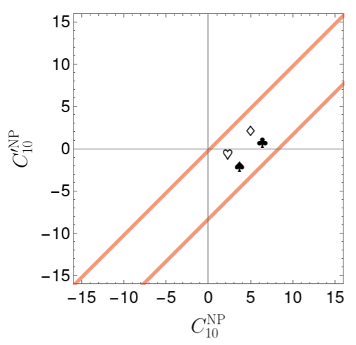
(a)

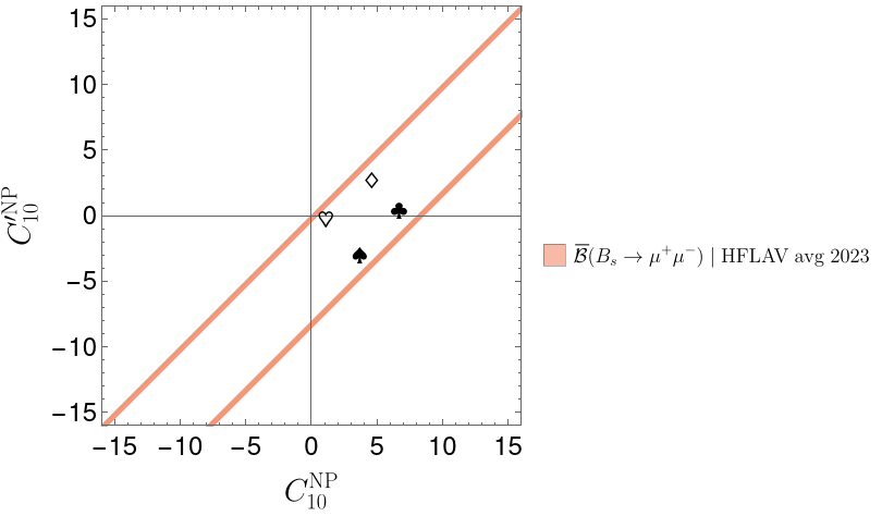
(b)

Figure 4: Constraints from the $B_{s}\to\mu^{+}\mu^{-}$ branching ratio on $C^{(\prime)\rm NP}_{10}$, assuming real coefficients and no (pseudo)-scalar NP. The inputs are specified in Sec. 2.2, and we use the hybrid/incl. CKM parameters in (31). The four points are the same as in Fig. 3.

4 Target Regions for New CP Violation in the (Pseudo)-Scalar Sector

4.1 Utilizing the Branching Ratio and $\mathcal{A}_{\Delta\Gamma_{s}}^{\mu\mu}$

Having obtained $\mathcal{C}^{-}_{10}$ through the semileptonic rare $B_{(s)}$ decays, we can now use the branching ratio and $\mathcal{A}_{\Delta\Gamma_{s}}^{\mu\mu}$ of the $B_{s}~{}\to~{}\mu^{+}\mu^{-}$ mode to determine $\mathcal{C}^{-}_{P}$ and $\mathcal{C}^{-}_{S}$, assuming both are real. As shown in Fig. 1, the branching ratio fixes a circular relation between $S$ and $P$. By using $\mathcal{C}^{-}_{10}$ as input, we obtain a relation between $\mathcal{C}^{-}_{P}$ and $\mathcal{C}^{-}_{S}$, illustrated in Fig. 5 for the four benchmark points in Table 2. Here we used the hybrid/incl. scenario for the CKM factors in (31) and the input parameters in Sec. 2.2. Since $B_{s}\to\mu^{+}\mu^{-}$ depends only on $\mathcal{C}^{-}_{10}$, points in the $C_{10}$–$C_{10}^{\prime}$ plane that lie on the same ascending diagonal will give the same circle. Thus, the four points only give two circles.

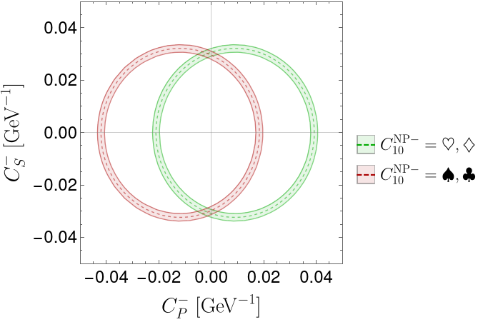
Figure 5: Allowed values of $\mathcal{C}^{-}_{P}$ and $\mathcal{C}^{-}_{S}$ following from the $B_{s}\to\mu^{+}\mu^{-}$ branching ratio using the hybrid/incl. CKM values in (31) The two circles correspond to different values of $\mathcal{C}_{10}^{-\rm NP}$, taken from Fig. 3(a), and represent the different intersections between contours coming from semileptonic rare $B$ decays.

Utilizing this relationship between $\mathcal{C}^{-}_{P}$ and $\mathcal{C}^{-}_{S}$, we can employ $\mathcal{A}_{\Delta\Gamma_{s}}^{\mu\mu}$ to determine their values. When $\mathcal{C}^{-}_{10}$ is real, $\mathcal{A}_{\Delta\Gamma_{s}}^{\mu\mu}$ fixes straight lines in the $\mathcal{C}^{-}_{P}$–$\mathcal{C}^{-}_{S}$ plane, as shown in [13] and illustrated in Fig. 66(a). Here we only show one value for $\mathcal{C}^{-}_{10}$, corresponding to the point marked by a heart in Fig. 3. We conclude that a measurement of $\mathcal{A}_{\Delta\Gamma_{s}}^{\mu\mu}$ can determine $\mathcal{C}^{-}_{P}$ and $\mathcal{C}^{-}_{S}$ up to a fourfold ambiguity. At the moment, we cannot constrain these contributions any further, although pioneering measurements of $\mathcal{A}_{\Delta\Gamma_{s}}^{\mu\mu}$ are already available through the $B_{s}\to\mu^{+}\mu^{-}$ effective lifetime (23). It will be interesting to see how future measurements of this observable will develop.

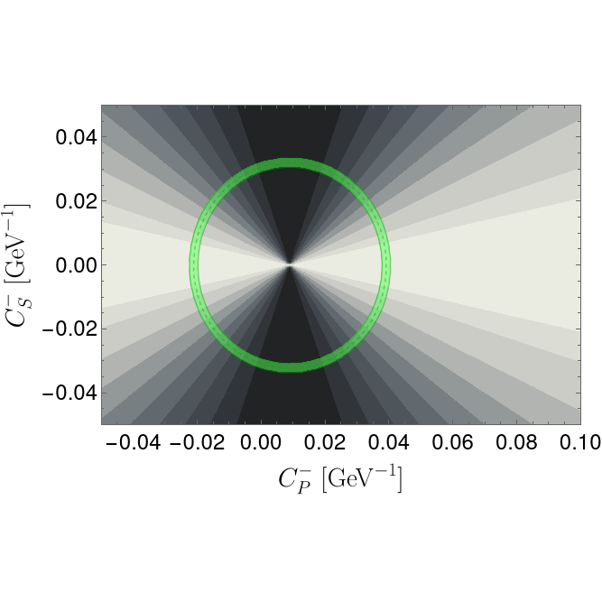
(a)

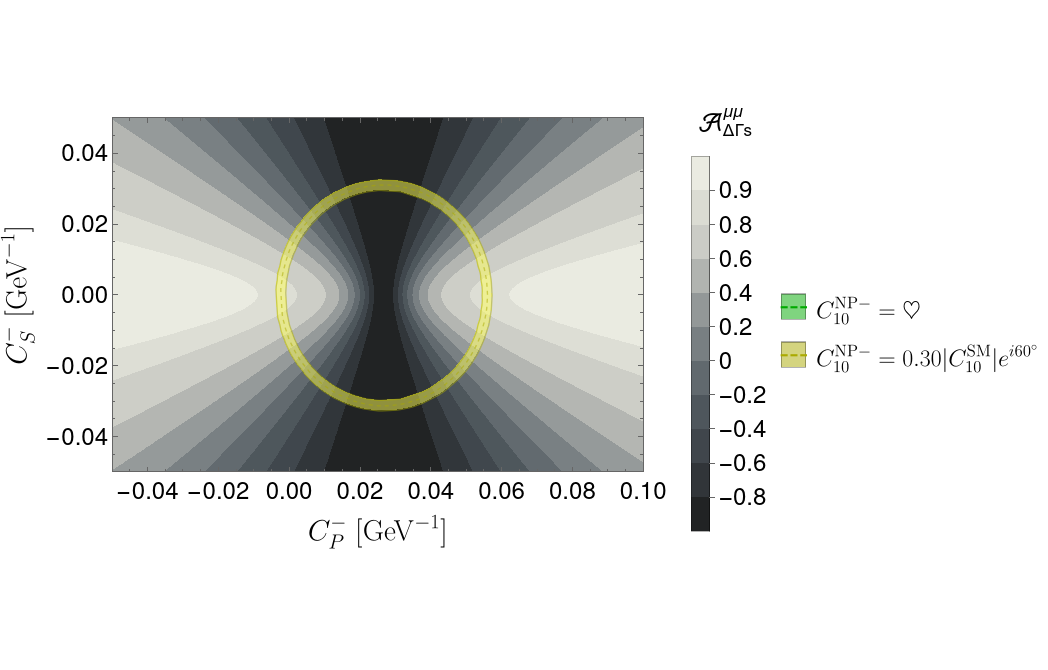
(b)

Figure 6: Values of $\mathcal{A}_{\Delta\Gamma_{s}}^{\mu\mu}$ in the $\mathcal{C}^{-}_{P}$–$\mathcal{C}^{-}_{S}$ plane for a real (a) and complex (b) $\mathcal{C}^{-}_{10}$. The circular bands show the $1\sigma$ regions consistent with the measurement of $\overline{\mathcal{B}}(B_{s}\to\mu^{+}\mu^{-})$ using the hybrid/incl. CKM values in (31).

If $\mathcal{C}^{-}_{10}$ is complex, the picture changes as we have illustrated in Fig. 66(b). Here, we assume the following benchmark scenario for $\mathcal{C}^{-}_{10}$:

$$\mathcal{C}_{10}^{-\rm NP} =0.30\absolutevalue{C_{10}^{\rm SM}}e^{i\>60^{\circ}}\ .$$ (50)

The circle indicates again the contour from the branching ratio, where in this case the point $\mathcal{C}^{-}_{S,P}=0$ is allowed because our benchmark point for $\mathcal{C}^{-}_{10}$ accommodates the current experimental branching ratio of $B_{s}\to\mu^{+}\mu^{-}$. Adding $\mathcal{A}_{\Delta\Gamma_{s}}^{\mu\mu}$ gives curved contours in the $\mathcal{C}^{-}_{P}$–$\mathcal{C}^{-}_{S}$ plane. We note that the value $\mathcal{A}_{\Delta\Gamma_{s}}^{\mu\mu}=1$ is excluded due to the complex value fixed for $\mathcal{C}^{-}_{10}$. The fact that now certain values of $\mathcal{A}_{\Delta\Gamma_{s}}^{\mu\mu}$ are excluded is an interesting new feature. Turning things around, with only real (pseudo)-scalar couplings, we can thus obtain a bound on $\mathcal{A}_{\Delta\Gamma_{s}}^{\mu\mu}$ from $\overline{\mathcal{B}}(B_{s}\to\mu^{+}\mu^{-})$ using (15). In this case, assuming $\varphi_{S}=0$ and using (9) we see that $\mathcal{C}^{-}_{10}$ will generate a non-trivial phase $\varphi_{P}\neq 0$. For the example in Fig. 66(b), we find $|\mathcal{A}_{\Delta\Gamma_{s}}^{\mu\mu}|<0.87$ within the branching ratio bound. We note that also in this case a measurement of $\mathcal{A}_{\Delta\Gamma_{s}}^{\mu\mu}$ can still be used to determine the Wilson coefficients $\mathcal{C}^{-}_{P}$ and $\mathcal{C}^{-}_{S}$.

4.2 Utilizing Mixing-Induced CP Violation

Additional information on possible new sources of CP violation comes from the mixing-induced CP asymmetry $\mathcal{S}_{\mu\mu}$ in (26). No measurements of $\mathcal{S}_{\mu\mu}$ are currently available; extracting it would require a time-dependent, flavour-tagged analysis as can be seen in (27).

We first consider real $\mathcal{C}^{-}_{10},\;\mathcal{C}^{-}_{P}$ and $\mathcal{C}^{-}_{S}$. In that case, we can only have a non-zero $\mathcal{S}_{\mu\mu}$ due to $\phi_{s}^{\rm NP}$ entering in (10). We then have

$$\mathcal{S}_{\mu\mu}=-\sin\phi_{s}^{\rm NP}\left(\frac{\absolutevalue{P}^{2}-\absolutevalue{S}^{2}}{\absolutevalue{P}^{2}+\absolutevalue{S}^{2}}\right)\ =[-0.062,0.062]\ ,$$ (51)

where we take $\phi_{s}^{\rm NP}$ from (19). The range indicates the extreme values reached for either $|S|=0$ or $|P|=0$. A measurement outside this range would clearly indicate additional sources of CP violation which could enter as complex phases in $\mathcal{C}^{-}_{10},\;\mathcal{C}^{-}_{P}$ and $\mathcal{C}^{-}_{S}$. By the time such a measurement is available, we will have a much sharper picture of $\phi_{s}^{\rm NP}$ from $B_{s}\to J/\psi\phi$ [26]. In addition, the semileptonic rare $B$ decays will allow a determination of $\mathcal{C}^{-}_{10}$. If this coupling is then found to be real, a measurement of $\mathcal{S}_{\mu\mu}$ would be crucial to find possible CP-violating (pseudo)-scalar interactions. In this case, a measurement outside the (updated) range in (51) would unambiguously indicate additional sources of new (pseudo)-scalar interactions.

However, measurements in the rare semileptonic $B$ decays could also result in a complex $\mathcal{C}^{-}_{10}$ (see e.g., [32]). This would be a more exciting situation, as then a new source of CP violation would already have been established. In this case, it would be important to explore whether also new (pseudo)-scalar interactions are present. In order to address this question, an analysis of $\mathcal{S}_{\mu\mu}$ and $\mathcal{A}_{\Delta\Gamma_{s}}^{\mu\mu}$ in $B_{s}\to\mu^{+}\mu^{-}$ will be crucial. As discussed in the previous subsection, in this case $\overline{\mathcal{B}}(B_{s}\to\mu^{+}\mu^{-})$ constrains a circle in the $\mathcal{C}^{-}_{P}$–$\mathcal{C}^{-}_{S}$ plane. Figure 77(a) shows this circle for our complex benchmark value of $\mathcal{C}_{10}^{-\rm NP}$ in (50). This constraint can be translated into the $\mathcal{A}_{\Delta\Gamma_{s}}^{\mu\mu}$–$\mathcal{S}_{\mu\mu}$ plane, yielding the red and blue C-shaped region in Fig. 77(b). The region shows which values of $\mathcal{A}_{\Delta\Gamma_{s}}^{\mu\mu}$ and $\mathcal{S}_{\mu\mu}$ are consistent with data on $\overline{\mathcal{B}}(B_{s}\to\mu^{+}\mu^{-})$ when $\mathcal{C}^{-}_{P}$ and $\mathcal{C}^{-}_{S}$ are real but $\mathcal{C}^{-}_{10}$ is complex. The resulting strong correlation between $\mathcal{A}_{\Delta\Gamma_{s}}^{\mu\mu}$ and $\mathcal{S}_{\mu\mu}$ provides a narrow target region for the search for new CP-violating sources that enter through the (pseudo)-scalar Wilson coefficients.

Moreover, if $\mathcal{C}^{-}_{P}$ and/or $\mathcal{C}^{-}_{S}$ have complex phases, $\mathcal{A}_{\Delta\Gamma_{s}}^{\mu\mu}$ and $\mathcal{S}_{\mu\mu}$ are no longer restricted to this region but can take any values within the unit disk. If future measurements were to fall outside the target region, we would have evidence for a complex phase in $\mathcal{C}^{-}_{P}$ and/or $\mathcal{C}^{-}_{S}$. In order to illustrate this exciting feature, we have marked four coloured points in Fig. 77(b) for several complex coefficients $\mathcal{C}^{-}_{P}$ and/or $\mathcal{C}^{-}_{S}$.

We conclude that through the surprisingly strong correlation between $\mathcal{A}_{\Delta\Gamma_{s}}^{\mu\mu}$ and $\mathcal{S}_{\mu\mu}$, we may reveal possible CP-violating effects in the (pseudo)-scalar sector.

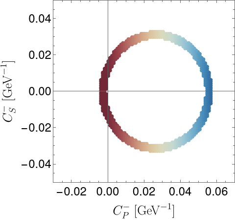
(a)

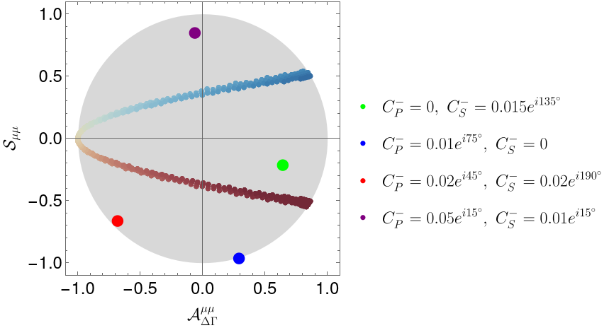
(b)

Figure 7: Correlations for the complex $\mathcal{C}^{-}_{10}$ benchmark scenario (50). (a) Constraints on real $\mathcal{C}^{-}_{P}$ and $\mathcal{C}^{-}_{S}$ from $\overline{\mathcal{B}}(B_{s}\to\mu^{+}\mu^{-})$, and (b) the corresponding correlation between $\mathcal{A}_{\Delta\Gamma_{s}}^{\mu\mu}$ and $\mathcal{S}_{\mu\mu}$ indicated with the same colour coding. The coloured points in (b) show the correlation for complex $\mathcal{C}^{-}_{P}$ and/or $\mathcal{C}^{-}_{S}$ which spans the whole unit disk as discussed in the text.

The method is robust with respect to the value of $\mathcal{C}^{-}_{10}$ extracted from the semileptonic $B$ decays. In Fig. 8, we show the target regions that result from three different values of $\mathcal{C}_{10}^{-\rm NP}$. This shows the power of this approach: after fixing $\mathcal{C}^{-}_{10}$, the branching ratio $\overline{\mathcal{B}}(B_{s}\to\mu^{+}\mu^{-})$ constrains a very specific region in the $\mathcal{A}_{\Delta\Gamma_{s}}^{\mu\mu}$–$\mathcal{S}_{\mu\mu}$ plane. Without fixing $\mathcal{C}^{-}_{10}$, the whole unit disk is allowed.

For completeness, we also consider the correlations with $\mathcal{C}_{\mu\mu}$, defined in (25). This observable, which is very challenging to measure, is only non-zero if scalar couplings are present. In Fig. 9, we show the unit spheres in the $\mathcal{A}_{\Delta\Gamma_{s}}^{\mu\mu}$–$\mathcal{S}_{\mu\mu}$–$\mathcal{C}_{\mu\mu}$ space for three different values of $\mathcal{C}^{-}_{10}$ given by (28). Again, the coloured contours are those allowed for real (pseudo)-scalar couplings coefficients. The projection along the $\mathcal{C}_{\mu\mu}$ axes corresponds to the 2D plots presented above.

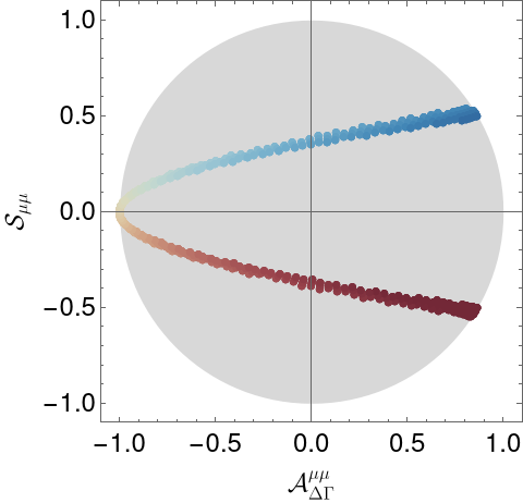
(a)

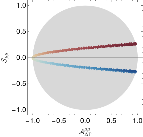
(b)

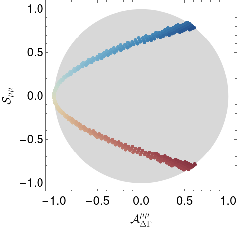
(c)

Figure 8: Correlations between $\mathcal{A}_{\Delta\Gamma_{s}}^{\mu\mu}$ and $\mathcal{S}_{\mu\mu}$ for different values of $\mathcal{C}^{-}_{10}$.

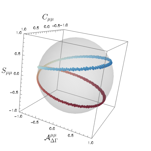
(a)

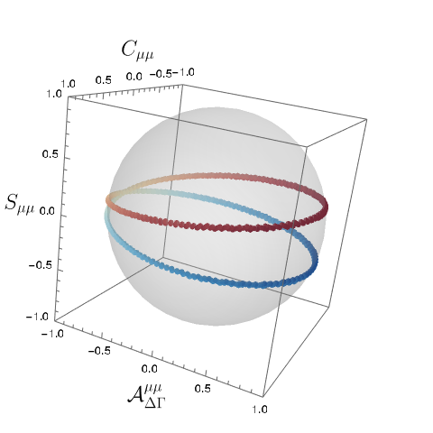
(b)

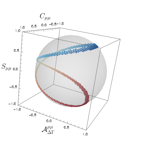
(c)

Figure 9: Illustration of the 3D correlations between $\mathcal{A}_{\Delta\Gamma_{s}}^{\mu\mu}$, $\mathcal{S}_{\mu\mu}$, and $\mathcal{C}_{\mu\mu}$ for different values of $\mathcal{C}^{-}_{10}$.

In summary, the strong correlation between $\mathcal{A}_{\Delta\Gamma_{s}}^{\mu\mu}$ and $\mathcal{S}_{\mu\mu}$, in combination with the branching ratio $\mathcal{B}(B_{s}\to\mu^{+}\mu^{-}$), allows us to detect the presence of possible CP-violating phases in $\mathcal{C}^{-}_{P}$ and/or $\mathcal{C}^{-}_{S}$. We illustrate the procedure in the flowchart of Fig. 10. Starting from the rare semileptonic decays, we can extract $\mathcal{C}^{-}_{10}$. This allows us to constrain a region in the $\mathcal{A}_{\Delta\Gamma_{s}}^{\mu\mu}$–$\mathcal{S}_{\mu\mu}$ plane. Once future data is available, as a final step, we can compare our target region with data to determine if there are new CP-violating contributions in the $\mathcal{C}^{-}_{S}$ and/or $\mathcal{C}^{-}_{P}$ coefficients.

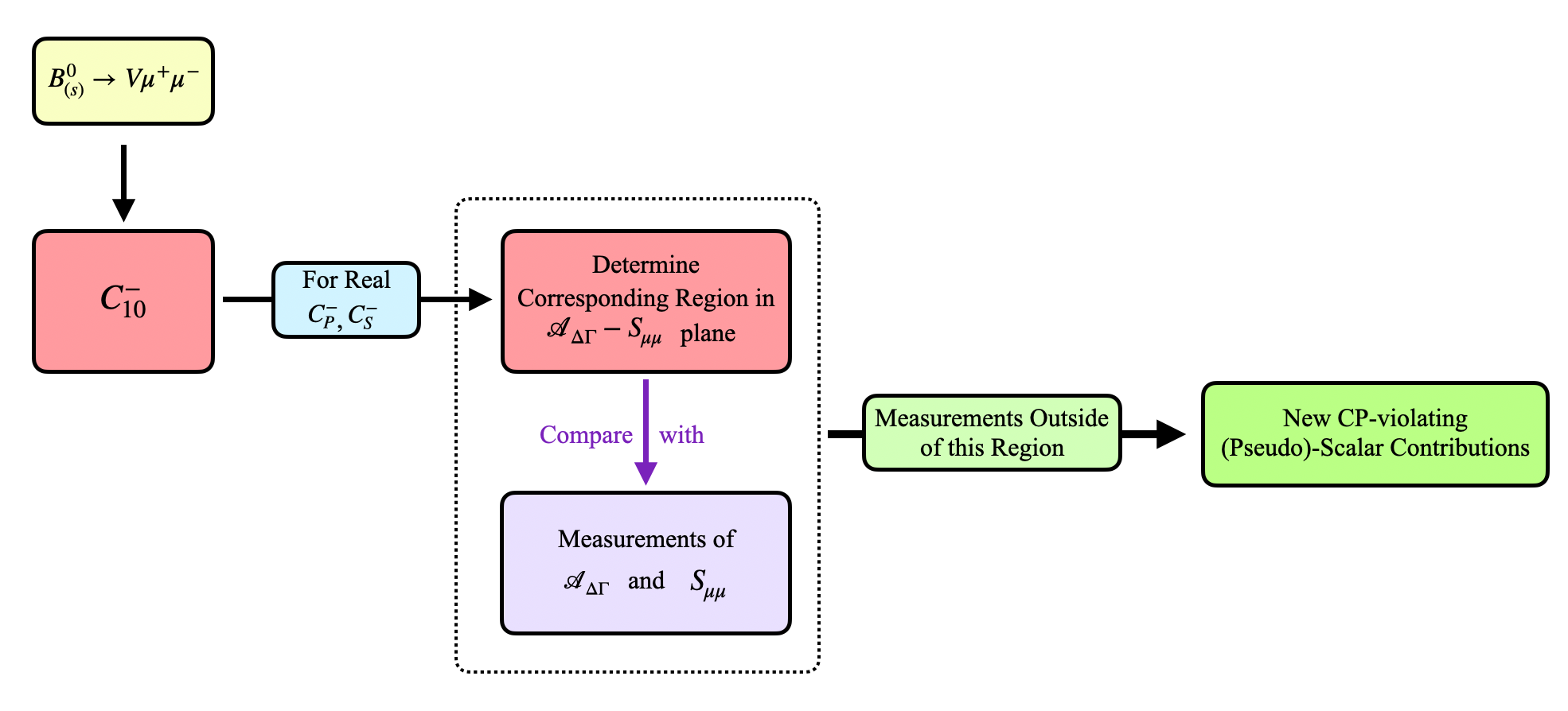
Figure 10: Illustration of our strategy to detect the presence of CP-violating phases in $\mathcal{C}^{-}_{P}$ and/or $\mathcal{C}^{-}_{S}$.

5 Conclusions and Outlook

We have presented a new strategy to determine whether there are new CP-violating (pseudo)-scalar interactions by fully exploiting the rare $B_{s}\to\mu^{+}\mu^{-}$ decay. We find that especially future measurements of the $\mathcal{A}_{\Delta\Gamma_{s}}^{\mu\mu}$ and $\mathcal{S}_{\mu\mu}$ observables have great potential in revealing New Physics.

In our method, we use $\mathcal{C}^{-}_{10}$ as an external input. We have demonstrated that the rare semileptonic $B_{(s)}\to K\mu^{+}\mu^{-}$ and $B\to K^{*}(\phi)\mu^{+}\mu^{-}$ decays are insensitive to new (pseudo)-scalar coefficients, which allows the extraction of $\mathcal{C}^{-}_{10}$. We then find surprisingly constrained target regions in the $\mathcal{A}_{\Delta\Gamma_{s}}^{\mu\mu}$–$\mathcal{S}_{\mu\mu}$ plane assuming NP entering in $\mathcal{C}^{-}_{P}$ and $\mathcal{C}^{-}_{S}$ to be CP-conserving. Moreover, any measurement outside these regions would indicate new CP-violating phases in the (pseudo)-scalar coefficients. This method provides an efficient way to identify possible new sources of CP violation in the (pseudo)-scalar sector.

Given the potential of CP-violating observables in $B_{s}\to\mu^{+}\mu^{-}$ to reveal NP, we strongly encourage the experimental community to perform the corresponding measurements. Pioneering, untagged time-dependent analyses of the effective lifetime by LHCb, ATLAS, and CMS are already available, leading to first determinations of $\mathcal{A}_{\Delta\Gamma_{s}}^{\mu\mu}$. As a next step, it would be crucial to perform also tagged time-dependent analyses, allowing the extraction of the observable $\mathcal{S}_{\mu\mu}$.

By the time these challenging measurements are available, we will have a clearer picture of possible NP effects. In particular, $\phi_{s}^{\rm NP}$ will have been constrained with much higher precision, which may even establish a non-zero value of that phase. Moreover, measurements in the semileptonic rare $B$ decays may already have brought us into the exciting scenario where NP effects are revealed in the coefficient $\mathcal{C}^{-}_{10}$. Either way, the observables in $B_{s}\to\mu^{+}\mu^{-}$ will play a key role in probing new CP-violating effects in (pseudo)-scalar interactions and determining the full dynamics of this rare decay.

References

- [1] Particle Data Group collaboration, R. L. Workman et al., Review of Particle Physics, PTEP 2022 (2022) 083C01.
- [2] CDF collaboration, T. Aaltonen et al., Search for and Decays with the Full CDF Run II Data Set, Phys. Rev. D 87 (2013) 072003, [1301.7048]. [Erratum: Phys.Rev.D 97, 099901 (2018)].
- [3] D0 collaboration, V. M. Abazov et al., Search for the Rare Decay , Phys. Rev. D 87 (2013) 072006, [1301.4507].
- [4] CMS, LHCb collaboration, V. Khachatryan et al., Observation of the rare decay from the combined analysis of CMS and LHCb data, Nature 522 (2015) 68–72, [1411.4413].
- [5] LHCb collaboration, R. Aaij et al., Measurement of the decay properties and search for the and decays, Phys. Rev. D 105 (2022) 012010, [2108.09283].
- [6] CMS collaboration, A. Tumasyan et al., Measurement of the B decay properties and search for the B0 decay in proton-proton collisions at = 13 TeV, Phys. Lett. B 842 (2023) 137955, [2212.10311].
- [7] ATLAS collaboration, M. Aaboud et al., Study of the rare decays of and mesons into muon pairs using data collected during 2015 and 2016 with the ATLAS detector, JHEP 04 (2019) 098, [1812.03017].
- [8] LHCb collaboration, R. Aaij et al., Physics case for an LHCb Upgrade II - Opportunities in flavour physics, and beyond, in the HL-LHC era, 1808.08865.
- [9] CMS collaboration, Measurement of decay properties and search for the decay in proton-proton collisions at , .
- [10] ATLAS collaboration, G. Aad et al., Measurement of the → effective lifetime with the ATLAS detector, JHEP 09 (2023) 199, [2308.01171].
- [11] K. De Bruyn, R. Fleischer, R. Knegjens, P. Koppenburg, M. Merk, A. Pellegrino et al., Probing New Physics via the Effective Lifetime, Phys. Rev. Lett. 109 (2012) 041801, [1204.1737].
- [12] R. Fleischer, D. G. Espinosa, R. Jaarsma and G. Tetlalmatzi-Xolocotzi, CP Violation in Leptonic Rare Decays as a Probe of New Physics, Eur. Phys. J. C 78 (2018) 1, [1709.04735].
- [13] R. Fleischer, R. Jaarsma and G. Tetlalmatzi-Xolocotzi, In Pursuit of New Physics with , JHEP 05 (2017) 156, [1703.10160].
- [14] C. Bobeth, M. Gorbahn, T. Hermann, M. Misiak, E. Stamou and M. Steinhauser, in the Standard Model with Reduced Theoretical Uncertainty, Phys. Rev. Lett. 112 (2014) 101801, [1311.0903].
- [15] W. Altmannshofer, C. Niehoff and D. M. Straub, as current and future probe of new physics, JHEP 05 (2017) 076, [1702.05498].
- [16] S. Descotes-Genon and J. Virto, Time dependence in decays, JHEP 04 (2015) 045, [1502.05509]. [Erratum: JHEP 07, 049 (2015)].
- [17] Flavour Lattice Averaging Group (FLAG) collaboration, Y. Aoki et al., FLAG Review 2021, Eur. Phys. J. C 82 (2022) 869, [2111.09849].
- [18] HPQCD collaboration, R. J. Dowdall, C. T. H. Davies, R. R. Horgan, C. J. Monahan and J. Shigemitsu, B-Meson Decay Constants from Improved Lattice Nonrelativistic QCD with Physical u, d, s, and c Quarks, Phys. Rev. Lett. 110 (2013) 222003, [1302.2644].
- [19] ETM collaboration, A. Bussone et al., Mass of the b quark and B -meson decay constants from Nf=2+1+1 twisted-mass lattice QCD, Phys. Rev. D 93 (2016) 114505, [1603.04306].
- [20] C. Hughes, C. T. H. Davies and C. J. Monahan, New methods for B meson decay constants and form factors from lattice NRQCD, Phys. Rev. D 97 (2018) 054509, [1711.09981].
- [21] A. Bazavov et al., - and -meson leptonic decay constants from four-flavor lattice QCD, Phys. Rev. D 98 (2018) 074512, [1712.09262].
- [22] A. J. Buras, R. Fleischer, J. Girrbach and R. Knegjens, Probing New Physics with the Time-Dependent Rate, JHEP 07 (2013) 077, [1303.3820].
- [23] D. M. Straub, flavio: a Python package for flavour and precision phenomenology in the Standard Model and beyond, 1810.08132.
- [24] HFLAV collaboration, Y. S. Amhis et al., Averages of -hadron, -hadron, and -lepton properties as of 2018, Eur. Phys. J. C81 (2021) 226, [1909.12524]. updated results and plots available at https://hflav.web.cern.ch/.
- [25] M. Z. Barel, K. De Bruyn, R. Fleischer and E. Malami, In pursuit of new physics with and decays at the high-precision Frontier, J. Phys. G 48 (2021) 065002, [2010.14423].
- [26] K. De Bruyn, R. Fleischer, E. Malami and P. van Vliet, New Physics in Mixing: Present Challenges, Prospects, and Implications for , J. Phys. G: Nucl. Part. Phys. (8, 2022) , [2208.14910].
- [27] M. Z. Barel, K. De Bruyn, R. Fleischer and E. Malami, Penguin Effects in and , in 11th International Workshop on the CKM Unitarity Triangle, 3, 2022. 2203.14652.
- [28] M. Bordone, B. Capdevila and P. Gambino, Three loop calculations and inclusive Vcb, Phys. Lett. B 822 (2021) 136679, [2107.00604].
- [29] HFLAV collaboration, Y. S. Amhis et al., Averages of b-hadron, c-hadron, and -lepton properties as of 2018, Eur. Phys. J. C 81 (2021) 226, [1909.12524].
- [30] M. Beneke, C. Bobeth and R. Szafron, Power-enhanced leading-logarithmic QED corrections to , JHEP 10 (2019) 232, [1908.07011]. [Erratum: JHEP 11, 099 (2022)].
- [31] Y. Amhis et al., Averages of -hadron, -hadron, and -lepton properties as of 2021, Phys. Rev. D 107 (2023) 052008, [2206.07501]. Online update at https://hflav.web.cern.ch/.
- [32] R. Fleischer, E. Malami, A. Rehult and K. K. Vos, Fingerprinting CP-violating New Physics with B → K+-, JHEP 03 (2023) 113, [2212.09575].
- [33] A. Bharucha, D. M. Straub and R. Zwicky, in the Standard Model from light-cone sum rules, JHEP 08 (2016) 098, [1503.05534].
- [34] N. Gubernari, M. Reboud, D. van Dyk and J. Virto, Improved theory predictions and global analysis of exclusive processes, JHEP 09 (2022) 133, [2206.03797].
- [35] LHCb collaboration, R. Aaij et al., Branching Fraction Measurements of the Rare and - Decays, Phys. Rev. Lett. 127 (2021) 151801, [2105.14007].
- [36] LHCb collaboration, R. Aaij et al., Differential branching fractions and isospin asymmetries of decays, JHEP 06 (2014) 133, [1403.8044].
- [37] C. Bobeth, M. Chrzaszcz, D. van Dyk and J. Virto, Long-distance effects in from analyticity, Eur. Phys. J. C 78 (2018) 451, [1707.07305].
- [38] A. K. Alok, B. Bhattacharya, A. Datta, D. Kumar, J. Kumar and D. London, New Physics in after the Measurement of , Phys. Rev. D 96 (2017) 095009, [1704.07397].
- [39] A. Datta, J. Kumar and D. London, The anomalies and new physics in , Phys. Lett. B 797 (2019) 134858, [1903.10086].
- [40] W. Altmannshofer and P. Stangl, New physics in rare B decays after Moriond 2021, Eur. Phys. J. C 81 (2021) 952, [2103.13370].
- [41] M. Algueró, J. Matias, B. Capdevila and A. Crivellin, Disentangling lepton flavor universal and lepton flavor universality violating effects in transitions, Phys. Rev. D 105 (2022) 113007, [2205.15212].
- [42] A. Carvunis, F. Dettori, S. Gangal, D. Guadagnoli and C. Normand, On the effective lifetime of Bs→ , JHEP 12 (2021) 078, [2102.13390].
- [43] F. Mahmoudi, Theoretical Review of Rare B Decays, in 20th Conference on Flavor Physics and CP Violation , 8, 2022. 2208.05755.
- [44] N. R. Singh Chundawat, violation in : a model independent analysis, 2207.10613.
- [45] S. Descotes-Genon, M. Novoa-Brunet and K. K. Vos, The time-dependent angular analysis of , a new benchmark for new physics, JHEP 02 (2021) 129, [2008.08000].