Fault Tolerance Embedded in a Quantum-Gap-Estimation Algorithm with Trial-State Optimization

Abstract

We construct a hybrid quantum algorithm to estimate gaps in many-body energy spectra and prove that it is inherently fault-tolerant to global multi-qubit depolarizing noise. Using trial-state optimization without active error correction, we show that the spectral peak of an exact target gap can be amplified beyond the noise threshold, thereby reducing gap-estimate error. We numerically verify fault tolerance using the Qiskit Aer simulator with a model of common mid-circuit noise channels. Our results reveal the potential for accurate quantum simulations on near-term noisy quantum computers.

Introduction.—Quantum simulation has been widely advertised as one of the most promising applications of a quantum computer. The exponential scaling of Hilbert space with a system size $N$ makes quantum simulation of many-body models on classical computers intractable beyond extremely limited system sizes. Applying quantum-phase-estimation (QPE) algorithms [1, 2, 3, 4], quantum computers can estimate the quantities of physical interest for many-body models, such as energy eigenvalues and gaps. In this application, quantum computers hold two distinct advantages over classical counterparts. Often promoted are advantages in computational time or circuit depth, however, quantum computers also pose an enormous memory advantage in that they naturally encode exponentially large Hilbert spaces in the hardware structure rather than storing them in classical random-access memory, thus avoiding the memory wall problem [5].

A primary goal of many-body quantum simulation is determining low-energy eigenstates which have widespread practical value in condensed matter physics [6, 7, 8], quantum chemistry [9, 10, 11], and materials science [12] due to the relevance of a ground state in determining material properties, reaction rates, and emergence of exotic phases such as superconductor. In general, preparing the ground state of a many-body model on a quantum computer is an NP-hard problem for classical Hamiltonians [13] and a QMA-hard problem for general quantum Hamiltonians [14, 15, 16]. Furthermore, the choice of initial states can have substantial impact on the performance of quantum simulation algorithms, and should be carefully considered when benchmarking algorithms.

Currently available quantum computers are noisy and limited in both qubit number (or circuit width) and circuit depth which pose significant challenges for conclusive demonstrations of quantum advantage in quantum simulation [17, 18]. The total number of gate operations, thus circuit depth, needed to achieve accurate phase estimation can be reduced by using variational methods [19, 20, 21, 22]. These approaches, however, provide only biased estimates of solutions and are not generally guaranteed to tolerate noise [23]. Alternatively, unbiased (exact) approaches, such as robust phase estimation [24] and quantum complex exponential least squares methods [25, 26], have demonstrated numerical evidence for robustness to some types of error [27, 28, 29]. Importantly, recent work [30] showed that, once a good approximation to a quantum state in the low-energy Hilbert space is found, Hamiltonian simulation stays in the same subspace in spite of noise.

Another promising avenue for improving circuit depth is the use of hybrid quantum algorithms in association with classical postprocessing [31, 32, 33, 34]. In our prior work [35], we proposed a hybrid quantum-gap-estimation (QGE) algorithm that combines time evolution on a quantum processor with classical signal processing to find the exact gaps in many-body energy spectra within a tolerance. In this method, a time series is constructed and filtered to exponentially improve circuit depth at the expense of spectral resolution. The operating range of the filter is determined by mapping out the input qubit orientations.

In this Letter, we construct a trial-state optimization method to maximize the performance of the hybrid QGE algorithm. Importantly, we prove that fault tolerance [36] is inherently embedded in the algorithm, thus yielding exact gaps of many-body models with error thresholds improved by updated trial states. Numerical verification is provided by running the algorithm for a minimal spin model on the Qiskit Aer simulator with a built-in noise model. This work opens the door to a significant boost in system size scaling that can be implemented on noisy intermediate-scale quantum computers [37], and lays the groundwork for demonstration of unbiased quantum simulation that outperforms classical approaches.

Trial-state optimization for QGE.—We present a hybrid QGE algorithm with a loop for trial-state optimization. Figure 1(a) describes the flowchart. In the quantum processor [Fig. 1(b)], each run is iterated over discrete time $t_{n}=n\delta t$, where $n\in[0,L-1]$, for Fourier sampling. For a single run, $N$ qubits are prepared or reset in the quantum registers, ($q_{0}$, $q_{1}$, $\cdots$, $q_{N-1}$), and rotated by the unitary $U_{\rm I}(\vec{\theta})$ to create a trial state with adjustable parameters $\vec{\theta}$ for optimization. Next, the trial state is time-evolved by the Trotterized unitary, e.g., of the first order [38, 39]: $U_{M}(t_{n})=(e^{-iH_{1}t_{n}/M}e^{-iH_{2}t_{n}/M})^{M}$, with Trotter depth $M$, which is a compact implementation of the exact time propagator $e^{-iHt_{n}}$ for a quantum many-body model $H=H_{1}+H_{2}$ with $[H_{1},H_{2}]\neq 0$. Last, the output state is rotated back to compensate $U_{\rm I}(\vec{\theta})$ and measured on the same circuit (without ancilla qubits) to return the diagonal components of the time propagator to the classical register, $c$.

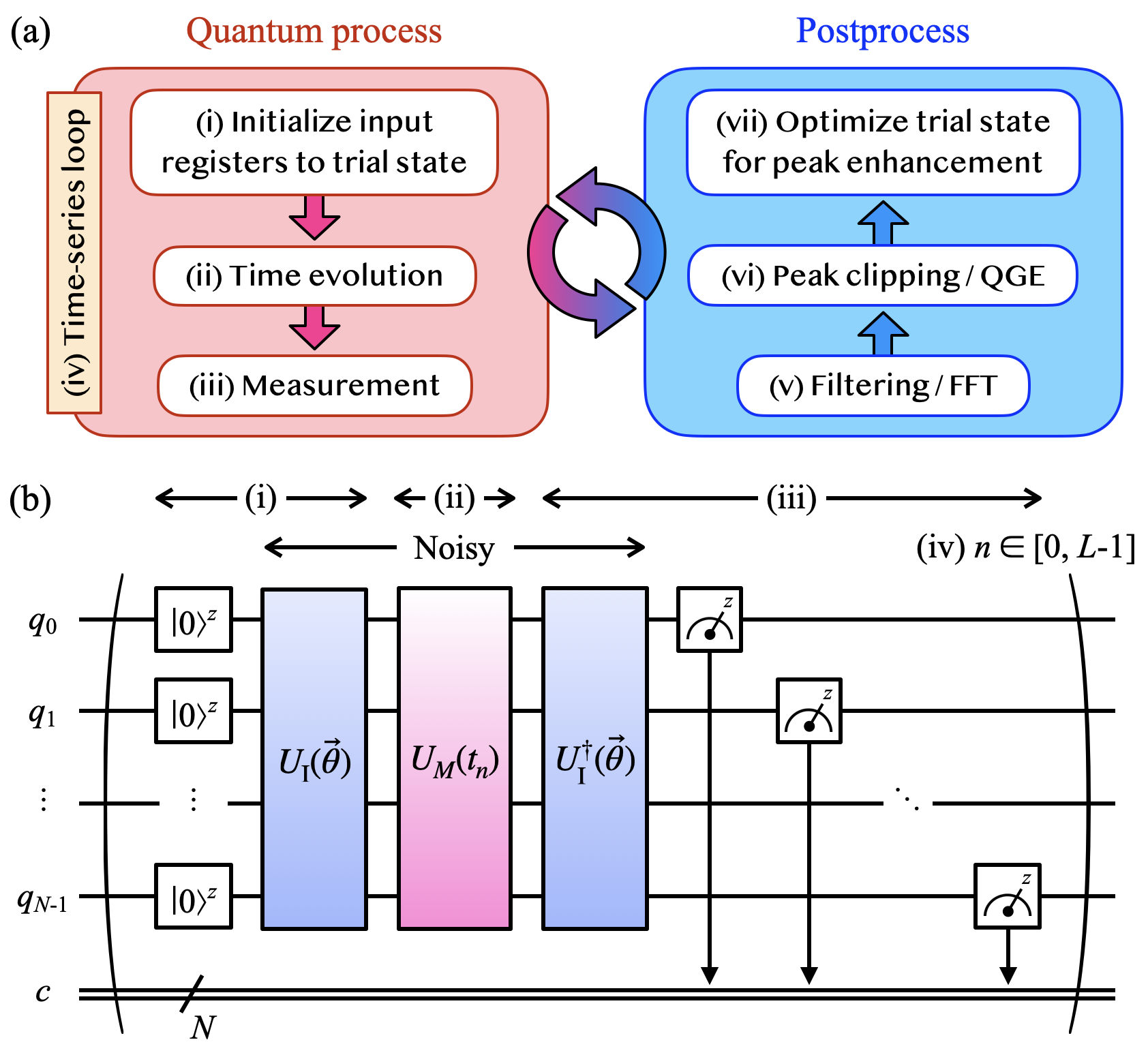
Figure 1: (a) Flowchart for the hybrid QGE algorithm with a loop for trial-state optimization. (b) Quantum circuit for (i) initialization to a trial state, (ii) time evolution, (iii) measurement. Here unitary gates are subject to noise. (iv) A time series of the propagators is constructed from measurement outcomes and (v)-(vii) postprocessed for gap estimation and trial-state optimization.

The output states are postprocessed to construct time-series data, $\{(t_{n},\mathcal{P}_{n})\}_{n=0}^{L-1}$. Here we define $z$-basis measurement outcomes: $\mathcal{P}_{n}={\rm Tr}[\rho_{0}\rho_{M,\vec{\theta}}(t_{n})]$ with the density matrices $\rho_{0}=\prod_{j=0}^{N-1}|0\rangle_{j}^{z}\langle 0|_{j}^{z}$ for the input registers and $\rho_{M,\vec{\theta}}(t_{n})=[U_{\rm I}(\vec{\theta})]^{\dagger}U_{M}(t_{n})U_{\rm I}(\vec{\theta})\rho_{0}[U_{\rm I}(\vec{\theta})]^{\dagger}[U_{M}(t_{n})]^{\dagger}U_{\rm I}(\vec{\theta})$ for the output state. The time series is filtered by $\mathcal{F}_{n}=\mathcal{F}(t_{n})$ satisfying $\mathcal{F}(t_{n}$ $\rightarrow\infty)\rightarrow 0$ to improve the performance of Fourier sampling and Trotterization [35], and fed into the classical subroutine for a fast Fourier transform (FFT) [40], which is promoted from a discrete Fourier transform yielding a spectral function:

$$\mathcal{A}(\omega_{m})=\frac{\delta t}{2\pi}{\rm Re}\sum_{s=\pm}\sum_{n=0}^{L-1}e^{i\omega_{m}t_{sn}}\mathcal{F}_{n}\mathcal{P}_{sn},$$ (1)

where we define discrete frequencies $\omega_{m}=m\delta\omega$, conjugate to $t_{n}$, in units of $\delta t$ and $\delta\omega$ satisfying $\delta\omega\delta t=2\pi/L$, $m,n\in[0,L-1]$, and $s$ counts the contributions from causal/anti-causal processes. Hereafter we drop discrete indices from $t_{n}$, $\omega_{m}$. Eq. (1) yields multiple peaks returning exact gaps from their centers. Once we set a target window to clip a peak from the full line shape for curve fitting, the energy gap is obtained from the peak center. Last, a classical optimizer is adopted to update trial-state parameters by maximizing the peak height. The optimization process continues until it meets convergence criteria within a tolerance.

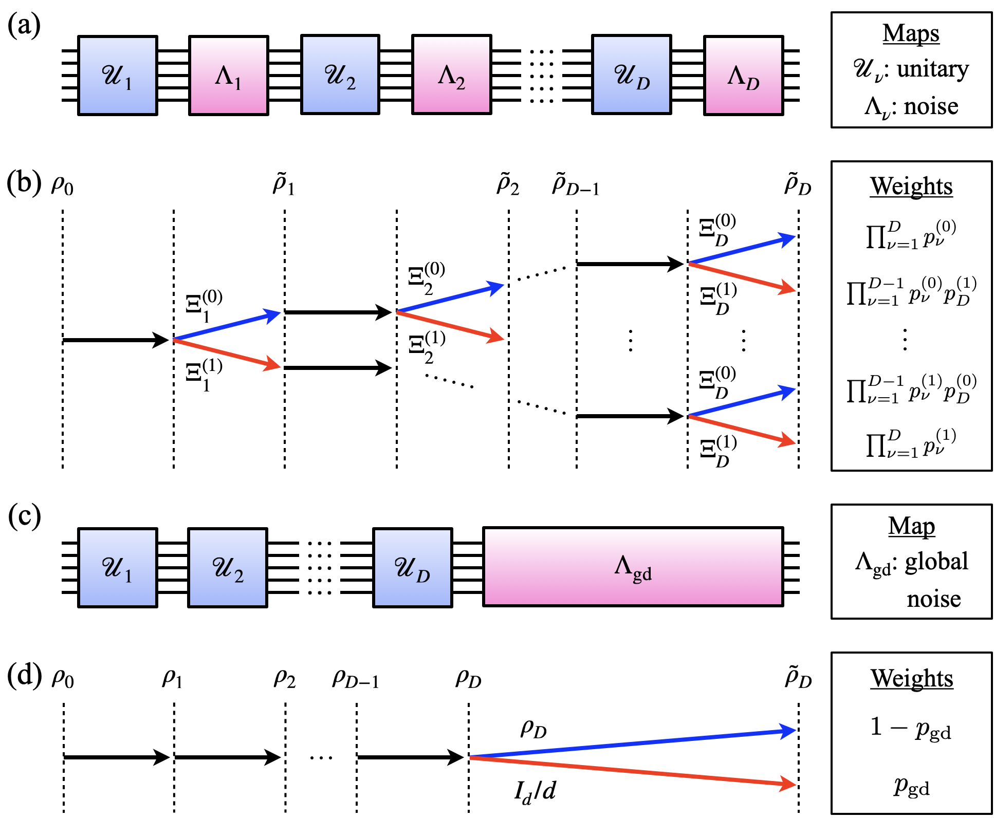
Figure 2: (a) Block diagram of a general noisy Trotterized circuit with the binary sequence of unitary/noise maps, $(\mathcal{U}_{\nu},\Lambda_{\nu})$ for $\nu\in[1,D]$. (b) Branching diagram showing all contributions to the noisy output density matrix $\tilde{\rho}_{D}$ arising from $\Lambda_{\nu}$ for multi-qubit depolarizing channel [Eq. (3)]. In each block, the black arrow indicates unitary evolution, and the blue (or red) arrow describes an idle process (or non-unitary evolution) with the probability $p_{\nu}^{(0)}$ (or $p_{\nu}^{(1)}$). The associated weights for available branches are listed in the right panel. (c) Equivalent block diagram to (a) but with the noise map $\Lambda_{\rm gd}$ for global depolarizing channel [Eq. (4)]. (d) Branching diagram for (c).

Fault tolerance embedded in QGE.—We prove that our hybrid QGE algorithm returns exact energy gaps in the presence of multi-qubit depolarizing noise. The proof relies on the fact that $e^{-iHt}$ applied to an arbitrary initial state oscillates in time at frequencies matching the exact gaps of $H$ [35]. To begin with, we allow arbitrary types of noise to arise at any stage in the quantum processes [Fig. 2(a)]. Ignoring temporal correlation (memory) between the processes at different stages [41], the noisy output state is described by the density matrix:

$$\tilde{\rho}_{D}=(\Lambda_{D}\circ\mathcal{U}_{D}\circ\cdots\circ\Lambda_{2}\circ\mathcal{U}_{2}\circ\Lambda_{1}\circ\mathcal{U}_{1})(\rho_{0}),$$ (2)

where, for $\nu\in[1,D]$, the unitary map $\mathcal{U}_{\nu}$ evolves $\rho$ to $U_{\nu}\rho U_{\nu}^{\dagger}$ with the unitary $U_{\nu}$ for either initialization or time evolution, and the (completely positive trace preserving) noise map $\Lambda_{\nu}$ describes non-unitary evolution of a quantum state by a certain type of noise channel.

For the $N$-qubit depolarizing channel, a compact analytic result can be derived. Since all branches of quantum processes cooperate to form a maximally mixed state, the noise map is significantly simplified into:

$$\Lambda_{\nu}(\rho)=p_{\nu}^{(0)}\Xi_{\nu}^{(0)}(\rho)+p_{\nu}^{(1)}\Xi_{\nu}^{(1)}(\rho),$$ (3)

where we define $\Xi_{\nu}^{(0)}(\rho)=\rho$, $\Xi_{\nu}^{(1)}(\rho)=I_{d}/d$, $I_{d}={\rm diag}(1,$ $1,\cdots,1)$ of size $d=2^{N}$, and $p_{\nu}^{(1)}$ is the depolarizing probability at stage $\nu$, satisfying $p_{\nu}^{(0)}+p_{\nu}^{(1)}=1$. Leveraging the structure of Eq. (3), we can count all contributions to Eq. (2) with the associated weights [Fig. 2(b)]. We then recast Eq. (2) into the equivalent form [Fig. 2(c-d)]:

$$\tilde{\rho}_{D} =(\Lambda_{\rm gd}\circ\mathcal{U}_{D}\circ\cdots\circ\mathcal{U}_{2}\circ\mathcal{U}_{1})(\rho_{0})$$

$$=(1-p_{\rm gd})(\mathcal{U}_{D}\circ\cdots\circ\mathcal{U}_{2}\circ\mathcal{U}_{1})(\rho_{0})+p_{\rm gd}I_{d}/d,$$ (4)

where $\Lambda_{\rm gd}$ defines the noise map for global depolarizing channel with the probability $p_{\rm gd}=1-\prod_{\nu=1}^{D}(1-p_{\nu}^{(1)})$. Plugging Eq. (4) in Eq. (1), we derive the noisy spectral function:

$$\tilde{\mathcal{A}}_{\rm gd}(\omega)=(1-p_{\rm gd})\mathcal{A}(\omega)+p_{\rm gd}\tilde{\mathcal{F}}(\omega)/d.$$ (5)

The noiseless part has the Lehmann representation: $\mathcal{A}(\omega)=\sum_{u,v}|c_{u}|^{2}|c_{v}|^{2}\tilde{\mathcal{F}}(\omega-\Delta_{u,v})$, where $\tilde{\mathcal{F}}(\omega-\Delta_{u,v})=\frac{1}{\pi}\int_{0}^{\infty}dt$ $\cos[(\omega-\Delta_{u,v})t]\mathcal{F}(t)$ and $\Delta_{u,v}=\mathcal{E}_{u}-\mathcal{E}_{v}$. In the derivation, we used $U_{D}\cdots U_{2}U_{1}=[U_{\rm I}(\vec{\theta})]^{\dagger}U_{M}(t)U_{\rm I}(\vec{\theta})$, $U_{M}(t)$ $=e^{-iHt}$ $+\mathcal{O}(t^{2}/M)$, and $|\psi_{\rm I}\rangle=U_{\rm I}(\vec{\theta})\prod_{j=0}^{N-1}|0\rangle_{j}^{z}=\sum_{u}$ $c_{u}|u\rangle$ with $|u\rangle$ satisfying $H|u\rangle=\mathcal{E}_{u}|u\rangle$. Peak heights in $\mathcal{A}$ are exponentially suppressed for increasing $D$, i.e., $1-p_{\rm gd}\approx e^{-Dp_{\rm dp}}$ for $p_{\rm dp}=p_{\nu}^{(1)}\ll 1$. Assuming that $Dp_{\rm dp}$ is bounded, this issue can be addressed by trial-state optimization for peak enhancement (as we discuss below). Noticeably, Eq. (5) tolerates the global depolarizing channel since the second term merely adds a redundant peak at $\omega=0$, which is ruled out in QGE. This is comparable to the robustness of data encodings for quantum classifiers against the same type of noise [42].

For non-depolarizing channels [43], the proof is highly non-trivial because the unitary and noise maps do not commute at every stage, and a more sophisticated approach is needed. We reserve this topic for future work [44]. In the following, we show simulation results for a minimal spin model to numerically confirm the fault tolerance to depolarizing noise and discuss the potential impact of non-depolarizing channels.

Simulation results for a minimal spin model.—For demonstration, we choose the transverse-field Ising model (TFIM) with open boundaries in one dimension:

$$H_{1}=-J\sum_{j=0}^{N-2}\sigma^{z}_{j}\sigma^{z}_{j+1},~{}H_{2}=-h\sum_{j=0}^{N-1}\sigma^{x}_{j},$$ (6)

where $(\sigma^{x},\sigma^{y},\sigma^{z})$ are the Pauli matrices, $N$ counts spins at sites $j\in[0,N-1]$, $J$ is the Ising coupling, and $h$ is the magnetic field. For quantum circuit implementation [Fig. 1(b)], the time-evolution unitary is specified by: $U_{M}(t)=\big{[}\prod_{j=0}^{N-2}$ $R_{j,j+1}^{zz}(-2Jt/M)\prod_{k=0}^{N-1}R_{k}^{x}(-2ht/M)\big{]}^{M}$, where we define one and two-qubit rotations $R_{j}^{\alpha_{j}}(\phi)=\exp(-i\frac{\phi}{2}\sigma_{j}^{\alpha_{j}})$ and $R_{j,j+1}^{\alpha_{j}\alpha_{j+1}}(\phi)=\exp(-i\frac{\phi}{2}\sigma_{j}^{\alpha_{j}}\sigma_{j+1}^{\alpha_{j+1}})$. On the other hand, the trial-state unitary is set to the form: $U_{\rm I}(\vec{\theta})=\prod_{j=0}^{N-1}R_{j}^{y}(\beta)$ $\prod_{k=0}^{N-2}R_{k,k+1}^{zz}(\gamma)$ with optimization parameters $\vec{\theta}=(\beta,\gamma)$. Our choice of $U_{\rm I}(\vec{\theta})$ is simpler (thus more scalable) than typical variational ansatzs [45] since its role is limited to peak enhancement via optimization of $U_{\rm I}(\vec{\theta})$.

Figure 3 shows simulation results for the TFIM of $N=5$, $J/h=0.4$ using the Qiskit Aer simulator (a) without [or (b) with] a noise model [46]. Success in our algorithm is subject to the protocols in classical signal processing. Specifically, a time series is filtered by a minimal model $\mathcal{F}_{\rm L}(t)=e^{-\eta t}$, and plugged in Eq. (1) to yield the spectral function $\mathcal{A}(\omega)$ [or $\tilde{\mathcal{A}}(\omega)$ including $\tilde{\mathcal{A}}_{\rm gd}(\omega)$] composed of multiple Lorentzian peaks with the line shape $\tilde{\mathcal{F}}_{\rm L}(\omega)=\frac{1}{\pi}\frac{\eta}{\omega^{2}+\eta^{2}}$ ($\eta>0$). Here we set $\eta/h=0.3$ to mitigate Trotter truncation error on shallow quantum circuits (here, $M=16$) [35]. The top panels describe the full line shape of $\mathcal{A}(\omega)$ [or $\tilde{\mathcal{A}}(\omega)$] at the first (dashed curve) and last (solid curve) iteration step for trial-state optimization. Here the redundant peak at $\omega=0$ was removed by curve fitting. Although the line shape contains all the information about energy gaps, separate protocols are still needed to correctly extract this information.

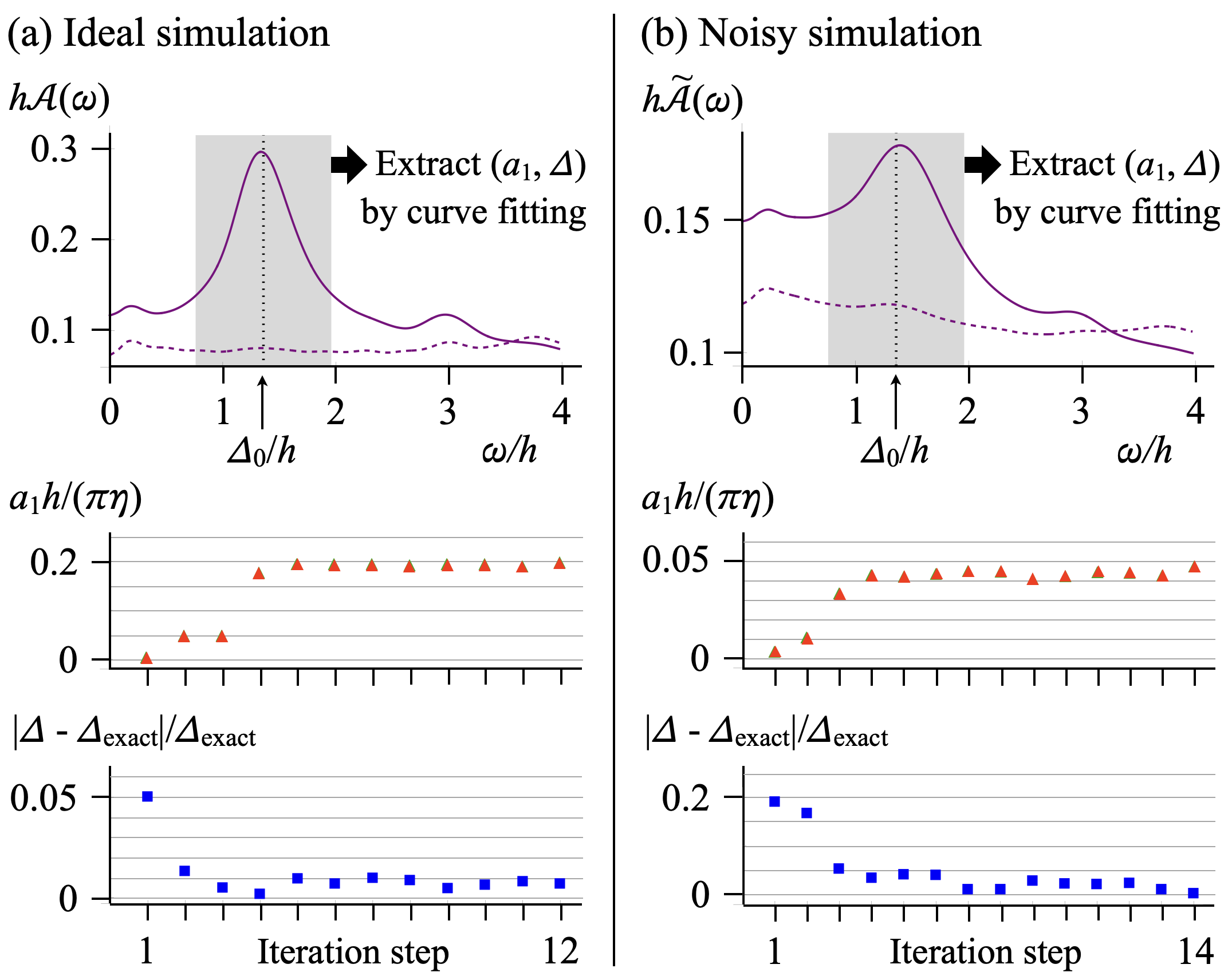
Figure 3: (a) Ideal and (b) noisy simulation results for the TFIM of $N=5$, $J/h=0.4$. Top panels: Spectral function $\mathcal{A}(\omega)$ [or $\tilde{\mathcal{A}}(\omega)$] at the first (dashed curve) and last (solid curve) iteration step for trial-state optimization. In postprocessing, a peak returning the first energy gap $\Delta_{\rm exact}(=\mathcal{E}_{2}-\mathcal{E}_{1})$ is targeted and clipped in the range $\Delta_{0}-\delta\Delta/2\leq\omega\leq\Delta_{0}+\delta\Delta/2$ (gray shading) with initial guess $\Delta_{0}$ (black vertical dotted line) and $\delta\Delta=4\eta$. The clipped peak is numerically fitted by the nonlinear model $a_{0}+a_{1}\tilde{\mathcal{F}}_{\rm L}(\omega-\Delta)$ to extract $(a_{0},a_{1},\Delta)$. In the classical optimizer, the Nelder-Mead method is adopted along with the cost function set to $-a_{1}h/(\pi\eta)$ and the trial-state parameters $(\beta,\gamma)$ initialized by $(0.5\pi,0.1\pi)$. Middle and bottom panels: Progress of $a_{1}h/(\pi\eta)$ and $|\Delta-\Delta_{\rm exact}|/\Delta_{\rm exact}$ as a function of the iteration step. In (a-b), we set parameters to $M=16$, $\eta/h=0.3$, $\delta\omega=\eta/4$, $L=2\lceil 7/\delta\omega\rceil$, $\varepsilon_{\rm op}=10^{-2}$, and measurement shots to $1024$ on the Qiskit Aer simulator. In (b), we set noise model parameters as shown in Table 1.

We demonstrate our gap estimation protocol with focus on the first energy gap $\Delta_{\rm exact}=\mathcal{E}_{2}-\mathcal{E}_{1}$. We start with an initial guess, $\Delta_{0}/h=2[1-(1-1/N)J/h]$, derived by perturbation theory for a quantum paramagnet. We then target and clip a peak in the range $\Delta_{0}-\delta\Delta/2\leq\omega\leq\Delta_{0}+\delta\Delta/2$. The window $\delta\Delta$ progressively increases until we reach a proper setup, here, $\delta\Delta=4\eta$. If $2\eta$ is comparable to peak-to-peak separations, the clipped peak center is potentially shifted from the exact location because the tail from neighbor peaks forms a slanted background around the peak of interest. Such an artifact can be relaxed by curve fitting. Here we use a nonlinear model $a_{0}+a_{1}h\tilde{\mathcal{F}}_{\rm L}(\omega-\Delta)$ with fitting parameters: offset $a_{0}(\geq 0)$, weight $a_{1}(\geq 0)$, and gap estimate $\Delta$. Last, we set the cost function to $-a_{1}h/(\pi\eta)$ (for peak enhancement), and the classical optimizer to the Nelder-Mead method [47], known to be heuristic but useful for nonlinear optimization problems with unknown derivatives. The trial-state parameters $(\beta,\gamma)$, initialized by $(0.5\pi,0.1\pi)$, stay updated by the classical optimizer until they meet convergence criteria within the tolerance $\varepsilon_{\rm op}=10^{-2}$.

The middle and bottom panels in Fig. 3 show the progress of the peak height $a_{1}h/(\pi\eta)$ and the gap-estimate error $|\Delta-\Delta_{\rm exact}|/\Delta_{\rm exact}$ as a function of the iteration step. For ideal simulation [Fig. 3(a)], we achieve an enormous 2516% peak enhancement after only 12 iterations, along with reasonable reduction of the gap-estimate error by 87.3%. As discussed above, $\mathcal{F}_{\rm L}(t)$ improves the Trotter truncation error but works within the operating range, i.e., $\eta$ bounded above from peak-to-peak separations. It turns out that $U_{\rm I}(\vec{\theta})$ impacts this range. Our result confirms that trial-state optimization improves the gap-estimate peak height by searching for the optimal choice of $U_{\rm I}(\vec{\theta})$. Advanced techniques in signal processing will further improve peak height  [48].

The last checkpoint is the applicability to noisy simulation. For demonstration, we adopt a model of common mid-circuit noise channels with the parameters imported from calibration data for the ibmq_manila processor (see Table 1). Figure 3(b) shows a remarkable peak enhancement of 950.3% and reduction of the gap-estimate error by 99.7%. This gives numerical evidence for fault tolerance to both non-depolarizing channels and global depolarizing channel. Noticeably, compared to the ideal case [Fig. 3(a)], peak enhancement is rather inhibited while the gap-estimate error is reduced more dramatically. The underlying reason is that the weight of the target peak is distributed to other satellite peaks (generated by non-depolarizing channels), actively growing slanted backgrounds behind the target peak and thus increasing the noise threshold. We confirm that trial-state optimization, without active error correction [49] or other error mitigation methods [50], successfully restores the peak center to the original location and significantly improves error thresholds.

(a)	(b)	(c)	(d)	(e)	(f)	(g)
0	65.16	18.13	5.700	5.700	0-1:7.997	0-1:277.3
1	208.8	63.37	3.243	3.243	1-2:18.01; 1-0:7.997	1-2:469.3; 1-0:312.9
2	147.7	17.26	2.435	2.435	2-3:6.517; 2-1:18.01	2-3:355.6; 2-1:504.9
3	182.0	60.76	1.617	1.617	3-4:4.992; 3-2:6.517	3-4:334.2; 3-2:391.1
4	77.88	37.82	4.111	4.111	4-3:4.992	4-3:298.7

Table 1: Calibration data of the ibmq_manila processor (with a linear array of 5 qubits, $q_{0}$–$q_{1}$–$q_{2}$–$q_{3}$–$q_{4}$). Here, each column denotes (a) qubit index, (b) $T_{1}$ ($\mu$s), (c) $T_{2}$ ($\mu$s), (d) $\sqrt{X}$ error ($\times 10^{-4}$), (e) Pauli-$X$ error ($\times 10^{-4}$), (f) CNOT error ($\times 10^{-3}$), (g) gate time (ns).

Conclusion.—We have developed a hybrid QGE algorithm that leverages classical signal processing for time-series filtering and iterative trial-state optimization to return unbiased gap estimates for quantum many-body models. We have analytically proven that the algorithm is inherently fault-tolerant in the presence of global multi-qubit depolarizing noise and demonstrated numerical evidence of tolerance to other noise channels through simulations on the Qiskit Aer simulator. In our numerical demonstration, we have found that, even in the presence of noise, trial-state optimization leads to an order of magnitude increase in the spectral peak height at the location of the target energy gap, thereby reducing the error in gap estimation.

These results open a significant number of avenues for future research and applications. In follow-up work [44], more complete analysis will be provided to support our numerical demonstration of the fault tolerance to non-depolarizing noise. Further analysis can examine the impact of realistic noise with memory [41] and the robust performance of our algorithm as the system size scales. Applications to other quantum many-body models beyond the TFIM can be explored as well. Notably, it is possible to extend the fault-tolerant structure of our algorithm to the estimation of other correlation functions associated with important physical observables beyond energy gaps, and further to other types of hybrid quantum algorithms that incorporate time-series analogs.

We acknowledge support from AFOSR (FA2386-21-1-4081, FA9550-19-1-0272, FA9550-23-1-0034) and ARO (W911NF2210247). We thank A. F. Kemper, P. Roushan, P. Alsing, S. Patel, and D. Koch for insightful discussion. We acknowledge the use of IBM Quantum services for this work. The views expressed are those of the authors, and do not reflect the official policy or position of IBM or the IBM Quantum team.

References

- Kitaev [1996] A. Kitaev, Quantum measurements and the Abelian stabilizer problem, Electr. Coll. Comput. Complex. TR96-003 (1996).
- Lloyd [1996] S. Lloyd, Universal quantum simulators, Science 273, 1073 (1996).
- Abrams and Lloyd [1999] D. S. Abrams and S. Lloyd, Quantum algorithm providing exponential speed increase for finding eigenvalues and eigenvectors, Phys. Rev. Lett. 83, 5162 (1999).
- Somma et al. [2002] R. Somma, G. Ortiz, J. E. Gubernatis, E. Knill, and R. Laflamme, Simulating physical phenomena by quantum networks, Phys. Rev. A 65, 042323 (2002).
- McKee and Wisniewski [2011] S. A. McKee and R. W. Wisniewski, Memory wall, in Encyclopedia of Parallel Computing, edited by D. Padua (Springer US, Boston, MA, 2011) pp. 1110–1116.
- Georgescu et al. [2014] I. M. Georgescu, S. Ashhab, and F. Nori, Quantum simulation, Rev. Mod. Phys. 86, 153 (2014).
- Reiner et al. [2019] J.-M. Reiner, F. Wilhelm-Mauch, G. Schön, and M. Marthaler, Finding the ground state of the Hubbard model by variational methods on a quantum computer with gate errors, Quantum Sci. Technol. 4, 035005 (2019).
- Stanisic et al. [2022] S. Stanisic, J. L. Bosse, F. M. Gambetta, R. A. Santos, W. Mruczkiewicz, T. E. O’Brien, E. Ostby, and A. Montanaro, Observing ground-state properties of the Fermi-Hubbard model using a scalable algorithm on a quantum computer, Nat. Commun. 13, 5743 (2022).
- Lanyon et al. [2010] B. P. Lanyon, J. D. Whitfield, G. G. Gillett, M. E. Goggin, M. P. Almeida, I. Kassal, J. D. Biamonte, M. Mohseni, B. J. Powell, M. Barbieri, A. Aspuru-Guzik, and A. G. White, Towards quantum chemistry on a quantum computer, Nat. Chem. 2, 106 (2010).
- Nam et al. [2020] Y. Nam, J.-S. Chen, N. C. Pisenti, K. Wright, C. Delaney, D. Maslov, K. R. Brown, S. Allen, J. M. Amini, J. Apisdorf, K. M. Beck, A. Blinov, V. Chaplin, M. Chmielewski, C. Collins, S. Debnath, K. M. Hudek, A. M. Ducore, M. Keesan, S. M. Kreikemeier, J. Mizrahi, P. Solomon, M. Williams, J. D. Wong-Campos, D. Moehring, C. Monroe, and J. Kim, Ground-state energy estimation of the water molecule on a trapped-ion quantum computer, npj Quantum Inf. 6, 33 (2020).
- Lee et al. [2023] S. Lee, J. Lee, H. Zhai, Y. Tong, A. M. Dalzell, A. Kumar, P. Helms, J. Gray, Z.-H. Cui, W. Liu, M. Kastoryano, R. Babbush, J. Preskill, D. R. Reichman, E. T. Campbell, E. F. Valeev, L. Lin, and G. K.-L. Chan, Evaluating the evidence for exponential quantum advantage in ground-state quantum chemistry, Nat. Commun. 14, 1952 (2023).
- Marzari et al. [2021] N. Marzari, A. Ferretti, and C. Wolverton, Electronic-structure methods for materials design, Nat. Mater. 20, 736 (2021).
- Poulin and Wocjan [2009] D. Poulin and P. Wocjan, Preparing ground states of quantum many-body systems on a quantum computer, Phys. Rev. Lett. 102, 130503 (2009).
- Kitaev et al. [2002] A. Y. Kitaev, A. H. Shen, and M. N. Vyalyi, Classical and Quantum Computation (American Mathematical Society, USA, 2002).
- Kempe et al. [2006] J. Kempe, A. Kitaev, and O. Regev, The complexity of the local Hamiltonian problem, SIAM J. Comput. 35, 1070 (2006).
- Aharonov et al. [2009] D. Aharonov, D. Gottesman, S. Irani, and J. Kempe, The power of quantum systems on a line, Commun. Math. Phys. 287, 41 (2009).
- Cao et al. [2019] Y. Cao, J. Romero, J. P. Olson, M. Degroote, P. D. Johnson, M. Kieferová, I. D. Kivlichan, T. Menke, B. Peropadre, N. P. D. Sawaya, S. Sim, L. Veis, and A. Aspuru-Guzik, Quantum chemistry in the age of quantum computing, Chem. Rev. 119, 10856 (2019).
- McArdle et al. [2020] S. McArdle, S. Endo, A. Aspuru-Guzik, S. C. Benjamin, and X. Yuan, Quantum computational chemistry, Rev. Mod. Phys. 92, 015003 (2020).
- Santagati et al. [2018] R. Santagati, J. Wang, A. A. Gentile, S. Paesani, N. Wiebe, J. R. McClean, S. Morley-Short, P. J. Shadbolt, D. Bonneau, J. W. Silverstone, D. P. Tew, X. Zhou, J. L. O’Brien, and M. G. Thompson, Witnessing eigenstates for quantum simulation of Hamiltonian spectra, Sci. Adv. 4, eaap9646 (2018).
- Wang et al. [2019] D. Wang, O. Higgott, and S. Brierley, Accelerated variational quantum eigensolver, Phys. Rev. Lett. 122, 140504 (2019).
- Filip et al. [2024] M.-A. Filip, D. M. Ramo, and N. Fitzpatrick, Variational phase estimation with variational fast forwarding, Quantum 8, 1278 (2024).
- Klymko et al. [2022] K. Klymko, C. Mejuto-Zaera, S. J. Cotton, F. Wudarski, M. Urbanek, D. Hait, M. Head-Gordon, K. B. Whaley, J. Moussa, N. Wiebe, W. A. de Jong, and N. M. Tubman, Real-time evolution for ultracompact Hamiltonian eigenstates on quantum hardware, PRX Quantum 3, 020323 (2022).
- Wang et al. [2024] S. Wang, P. Czarnik, A. Arrasmith, M. Cerezo, L. Cincio, and P. J. Coles, Can error mitigation improve trainability of noisy variational quantum algorithms?, Quantum 8, 1287 (2024).
- Kimmel et al. [2015] S. Kimmel, G. H. Low, and T. J. Yoder, Robust calibration of a universal single-qubit gate set via robust phase estimation, Phys. Rev. A 92, 062315 (2015).
- Ding and Lin [2023a] Z. Ding and L. Lin, Even shorter quantum circuit for phase estimation on early fault-tolerant quantum computers with applications to ground-state energy estimation, PRX Quantum 4, 020331 (2023a).
- Ding and Lin [2023b] Z. Ding and L. Lin, Simultaneous estimation of multiple eigenvalues with short-depth quantum circuit on early fault-tolerant quantum computers, Quantum 7, 1136 (2023b).
- Meier et al. [2019] A. M. Meier, K. A. Burkhardt, B. J. McMahon, and C. D. Herold, Testing the robustness of robust phase estimation, Phys. Rev. A 100, 052106 (2019).
- Russo et al. [2021] A. E. Russo, K. M. Rudinger, B. C. A. Morrison, and A. D. Baczewski, Evaluating energy differences on a quantum computer with robust phase estimation, Phys. Rev. Lett. 126, 210501 (2021).
- Ding et al. [2023] Z. Ding, Y. Dong, Y. Tong, and L. Lin, Robust ground-state energy estimation under depolarizing noise, arXiv:2307.11257 [quant-ph] (2023).
- Şahinoğlu and Somma [2021] B. Şahinoğlu and R. D. Somma, Hamiltonian simulation in the low-energy subspace, npj Quantum Inf. 7 (2021).
- O’Brien et al. [2019] T. E. O’Brien, B. Tarasinski, and B. M. Terhal, Quantum phase estimation of multiple eigenvalues for small-scale (noisy) experiments, New J. Phys. 21, 023022 (2019).
- Wan et al. [2022] K. Wan, M. Berta, and E. T. Campbell, Randomized quantum algorithm for statistical phase estimation, Phys. Rev. Lett. 129, 030503 (2022).
- Dutkiewicz et al. [2022] A. Dutkiewicz, B. M. Terhal, and T. E. O’Brien, Heisenberg-limited quantum phase estimation of multiple eigenvalues with few control qubits, Quantum 6, 830 (2022).
- Lin and Tong [2022] L. Lin and Y. Tong, Heisenberg-limited ground-state energy estimation for early fault-tolerant quantum computers, PRX Quantum 3, 010318 (2022).
- Lee et al. [2024] W.-R. Lee, R. Scott, and V. W. Scarola, Hybrid quantum-gap-estimation algorithm using a filtered time series, Phys. Rev. A 109, 052403 (2024).
- Katabarwa et al. [2023] A. Katabarwa, K. Gratsea, A. Caesura, and P. D. Johnson, Early fault-tolerant quantum computing, arXiv:2311.14814 [quant-ph] (2023).
- Preskill [2018] J. Preskill, Quantum computing in the NISQ era and beyond, Quantum 2, 79 (2018).
- Trotter [1959] H. F. Trotter, On the product of semi-groups of operators, Proc. Am. Math. Soc. 10, 545 (1959).
- Suzuki [1976] M. Suzuki, Generalized Trotter’s formula and systematic approximants of exponential operators and inner derivations with applications to many-body problems, Commun. Math. Phys. 51, 183 (1976).
- Duhamel and Vetterli [1990] P. Duhamel and M. Vetterli, Fast fourier transforms: A tutorial review and a state of the art, Signal Process. 19, 259 (1990).
- Breuer et al. [2016] H. P. Breuer, E. M. Laine, J. Piilo, and B. Vacchini, Colloquium: Non-Markovian dynamics in open quantum systems, Rev. Mod. Phys. 88, 021002 (2016).
- LaRose and Coyle [2020] R. LaRose and B. Coyle, Robust data encodings for quantum classifiers, Phys. Rev. A 102, 032420 (2020).
- Siudzińska [2020] K. Siudzińska, Classical capacity of generalized pauli channels, J. Phys. A Math. Theor. 53, 445301 (2020).
- [44] N. M. Myers, W.-R. Lee, and V. W. Scarola, unpublished .
- Tilly et al. [2022] J. Tilly, H. Chen, S. Cao, D. Picozzi, K. Setia, Y. Li, E. Grant, L. Wossnig, I. Rungger, G. H. Booth, and J. Tennyson, The variational quantum eigensolver: A review of methods and best practices, Phys. Rep. 986, 1 (2022).
-
[46]
QISKIT code for the hybrid QGE algorithm,
https://github.com/
wrlee7609/hybrid_quantum_gap_estimation. - Nelder and Mead [1965] J. A. Nelder and R. Mead, A simplex method for function minimization, Comput. J. 7, 308 (1965).
- Esakkirajan et al. [2024] S. Esakkirajan, T. Veerakumar, and B. N. Subudhi, Digital Signal Processing: Illustration Using Python (Springer, 2024).
- Terhal [2015] B. M. Terhal, Quantum error correction for quantum memories, Rev. Mod. Phys. 87, 307 (2015).
- Cai et al. [2023] Z. Cai, R. Babbush, S. C. Benjamin, S. Endo, W. J. Huggins, Y. Li, J. R. McClean, and T. E. O’Brien, Quantum error mitigation, Rev. Mod. Phys. 95, 045005 (2023).