On Sample Selection for Continual Learning:
a Video Streaming Case Study

Abstract.

Machine learning (ML) is a powerful tool to model the complexity of communication networks. As networks evolve, we cannot only train once and deploy. Retraining models, known as continual learning, is necessary. Yet, to date, there is no established methodology to answer the key questions:
With which samples to retrain? When should we retrain?

We address these questions with the sample selection system Memento, which maintains a training set with the “most useful” samples to maximize sample space coverage. Memento particularly benefits rare patterns—the notoriously long “tail” in networking—and allows assessing rationally when retraining may help, i.e., when the coverage changes.

We deployed Memento on Puffer, the live-TV streaming project, and achieved a $14\text{\,}\mathrm{\char 37\relax}$ reduction of stall time, $3.5\times$ the improvement of random sample selection. Since Memento does not depend on a specific model architecture, it is likely to yield benefits in other ML-based networking applications.

1. Introduction

Adaptive Bit Rate (ABR) algorithms aim to avoid video stalls while maximizing the image quality in video streaming. This entails predicting the transfer time of video chunks, a complex task for which researchers are increasingly using machine learning (ML) (yanLearningSituRandomized2020, ; maoNeuralAdaptiveVideo2017, ; xiaAutomaticCurriculumGeneration2022, ). Current ML-based ABR algorithms already achieve good average performance; i.e., high image quality while largely avoiding stalls (yanLearningSituRandomized2020, ; langleyQUICTransportProtocol2017, ). But rare stalls matter as they are known to impact user experience far more than image quality (duanmuQualityofExperienceIndexStreaming2017, ; krishnanVideoStreamQuality2013, ). Moreover, as networks evolve, maintaining performance over time is a concern that hinders the deployment of ML-based solutions. This challenge is known as continual learning (parisiContinualLifelongLearning2019, ; buzzegaRethinkingExperienceReplay2020, ; iseleSelectiveExperienceReplay2018, ; rolnickExperienceReplayContinual2019, ).

In this paper, we ask if and how we can improve tail performance over time while maintaining the average. For ABR, this translates to reducing stalls while maintaining quality.

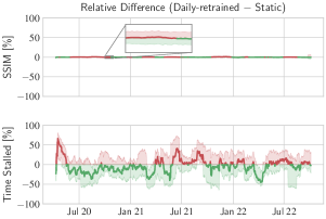
Figure 1. On Puffer (Puffer, ), retraining daily with random samples did not outperform a never-retrained model consistently. On average, image quality and stream-time spent stalled differ by less than $0.2\text{\,}\mathrm{\char 37\relax}$ and $4.2\text{\,}\mathrm{\char 37\relax}$.
Mean and 90% CI over a one-month sliding window. Data source: (Puffer, )

The most common approach to improve ML performance is using more: more data, more training, more complex models. However, this does not guarantee (tail) improvements. More training does not help if done using the wrong samples. Similarly, naively using more data does not improve tail performance if it does not address the imbalance between average and tail samples. Finally, more models can help to address this if they cover different parts of the data distribution. Otherwise, the individual models fail to complement each other and provide no benefit. Besides its uncertain effectiveness, using more increases training and inference time. For large networking applications, this can be significant. If YouTube were to use ML-based ABR, it would require inference for $\approx$30 billion video chunks per day (YouTubeStatistics20242024, ): slower inference means higher costs in delay, energy, and money.

Instead of using more, we propose to improve performance with a smarter selection of training samples, which we motivate with the following case study.

Puffer case study

The best study of continual learning in networking to date is Puffer (Puffer, ). This ongoing study monitors ABR performance with users streaming live TV with randomly assigned algorithms. Puffer’s authors proposed their own ML-based ABR and retrained it daily using random samples from the past two weeks (Fig. 1).

To the author’s surprise (yanLearningSituRandomized2020, ), retraining every day brought essentially no benefits: Over almost $900$ days, it improved image quality by only $0.17\text{\,}\mathrm{\char 37\relax}$ over a static—never retrained—version (Fig. 1, top). On the tail, daily retraining reduced the fraction of stream time spent stalled by $4.17\text{\,}\mathrm{\char 37\relax}$ on average, with large fluctuations over time (Fig. 1, bottom). This illustrates the more training approach falling short. But why? Why is the daily-retrained model not consistently outperforming the static one? Why does it stall only half the time in some months but twice as much in others (Fig. 1, bottom)?

We argue retraining did not help because training samples were selected randomly. As most streaming sessions perform similarly, this leads to an imbalanced training set with many similar samples and few tail ones. Doubling the number of training samples in the same setup—more data—does not help either (Fig. 2): we must address this imbalance to improve a model’s tail performance. Query-By-Committee (QBC) (seungQueryCommittee1992, ) is a classic approach to address such imbalance by selecting samples where a committee of models disagrees and prediction entropy is high. When applying QBC to the Puffer data, we observe that the models fail to identify rare samples reliably and eventually overfit on noise (Fig. 2), i.e., using more models is not enough to improve tail performance.

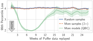
Figure 2. More resources do not guarantee better tail performance. Using more random samples has virtually no effect. Using more models to select training samples (QBC) initially helps but degrades over time.
Mean and 90% CI over a two-week sliding window (see Section 4 for details).

Problem

Fig. 1 and Fig. 2 suggest that retraining can improve tail performance, but we observe common approaches like random sampling or QBC to be ineffective or unreliable over time. If the selection got lucky, retraining improved the tail; other times, retraining was useless or even detrimental. We argue that we can do better with a smarter selection strategy that reliably picks up important tail samples. In summary, we must answer the following two questions:

1. From a stream of new samples, with which samples should we retrain to improve performance over time?

2. From an updated set of training samples in memory, when should we retrain the model? Given the large resource costs, can we avoid retraining “for nothing”?

Fundamentally, an algorithm addressing these questions requires: (i) a signal to select important samples, able to identify the tail; (ii) a signal to quantify changes to decide when to retrain; (iii) a mechanism to forget noise and outdated samples to avoid degradation over time (QBC in Fig. 2). Finally, resource usage should be small compared to using more.

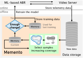
Figure 3. Memento maximizes sample space coverage, improving the tail while rationalizing when to retrain.

Solution

We propose a sample-space-aware continual learning algorithm based on coverage maximization, i.e., prioritizing samples from low-density areas of the sample space, and present Memento, a prototype implementation of this idea. Fig. 3 illustrates how Memento integrates with an ML-based video streaming system transmitting videos in chunks. In ML-based ABR, a sample encompasses telemetry data for recent video chunks; samples are collected by the server.

Memento estimates the sample-space density from both new and in-memory samples, prioritizing rare low-density samples to address dataset imbalance and improve tail performance. Memento uses the difference in coverage to assess whether there is something new to learn. If so, it retrains.

Main contributions

• We propose a sample-space-aware continual learning algorithm using density to improve tail performance.

• We present Memento (Fig. 3), a prototype implementation that uses sample-space density for sample selection. Memento is publicly available (Appendix A).

• We validate the effectiveness of our algorithm by applying Memento on an extensive ABR case study.

  • We deployed Memento on Puffer and collected $10$ stream-years of real-world data over $9$ months.

  • Memento stalls $14\text{\,}\mathrm{\char 37\relax}$ less than the static model ($3.5$$\times$ better than daily retraining with random samples).

  • Memento achieves this by retraining only $7$ times with a marginal degradation on image quality ($0.13\text{\,}\mathrm{\char 37\relax}$).

  • Memento has easy-to-tune parameters.

• We conduct microbenchmarks using data center workloads to show that out algorithm is not limited to ABR.

2. A case for density

We propose a continual learning algorithm based on estimating sample space density. Estimating density allows the algorithm to prioritize rare low-density samples, ultimately maximizing the sample space coverage. This section provides intuition as to why we propose this selection metric instead of per-sample metrics like sample loss or QBC’s entropy.

Density for sample selection

“The tail” is not a single pattern that rare traffic follows, but rather many patterns with only a few samples each. A random sample selection mirrors any imbalance in the underlying distribution, e.g., over-represented common traffic patterns. This leads to diminishing returns as we sample more and more from common patterns and little from the tail. As illustrated by Fig. 1, this yields good average performance but is unreliable at the tail. We need to address the imbalance of the training set.

To correct dataset imbalance, we need a sample-space-aware selection. Traditional approaches use the model performance (e.g., entropy, loss, reward) to select samples (buzzegaRethinkingExperienceReplay2020, ; iseleSelectiveExperienceReplay2018, ). We found that this does not work well on Puffer because it fails to avoid catastrophic forgetting. By considering each sample independently, they fail to preserve samples with good performance representing ‘normal’ traffic.

Instead, we propose to select samples based on the density of their neighborhood, which considers the whole sample space: a sample-space-aware selection that aims to maximize coverage of the sample space. The key insight to maximize coverage is to retain samples where few similar samples exist. We achieve this by removing samples from high-density areas with the most similar samples. This decreases the density and we naturally stop removing further samples.

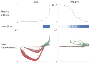
Figure 4. Loss improvement obtained by retaining with 1M samples over a dataset of 5M. The same batches of 256 samples are used for the loss- (left) and density-based selection (right).
To improve tail performance, we need many low-density batches because they are all different. To maintain average performance, we need only a few high-density batches, as they are similar. Selecting based on density (right) achieves both. Conversely, loss-based selection (left) is too specific. It suffers from diminishing returns by selecting too many high-loss batches and catastrophically forgets the average.

Fig. 4 illustrates the benefits of samples-space-aware density versus sample-aware loss as a selection metric. In this experiment, we use the static model from Puffer’s authors and $5\text{\,}\mathrm{M}$ samples collected by Puffer over a few days. We create batches of 256 samples and compute their loss and density (as detailed in Section 3). The top row of Fig. 4 shows the mean loss and density per batch. We then use each metric to select $1\text{\,}\mathrm{M}$ samples and retrain the model. The bottom row compares the effect of each selection metric over the $5\text{\,}\mathrm{M}$ samples by showing the mean loss improvement per batch.

The left column shows that loss-based selection focuses too much on the tail, i.e., high-loss batches. It yields good improvements there but does not preserve enough average samples and degrades performance on most other batches.

Conversely, the right column illustrates that density-based selection is more holistic, focusing on the tail while covering the entire sample space. Performance is improved at the tail, i.e., on low-density batches, without much degradation on the high-density ones. One may object that the loss selection could be tuned to maintain more “low-loss samples.” We tried this and our evaluation shows that it does not perform as well as density and can easily get much worse (Sections 4.4 and 8).

These results also shed some light on why we observed QBC degrade over time (Section 1, Fig. 2). Overall, QBC has some inertia, as models are gradually replaced (more details in Section 4.4), but we ultimately observe a similar effect as loss-based selection. Noisy samples are, by definition, random and have high entropy. Consequently, they are preferred by QBC. Over time, QBC accumulates noise and forgets the average and more common tail samples. As a result, it is unable to maintain the initial performance improvements on the tail.

Density for shift detection

Continual learning aims to adapt when the data distribution changes. These changes can be broadly categorized into covariate shift (shimodairaImprovingPredictiveInference2000, ), i.e., previously unseen traffic patterns emerge or the prevalence of patterns changes and concept drift (widmerLearningPresenceConcept1996, ), i.e., the underlying network dynamics change. Density-based sample selection is an effective tool to capture both kinds of changes.

When new traffic patterns appear, e.g., users starting to stream over satellite networks, they populate a previously-empty area of the sample space, resulting in a low density and, thus, a high probability of being selected for retraining. Similarly, patterns becoming less prevalent results in low density, and a high probability of remaining selected.

When the underlying network dynamics change, e.g., a new congestion control gets deployed, we should forget old samples that are no longer relevant. However, detecting those changes is difficult, and being wrong risks forgetting useful information such as hard-to-gather tail samples.

Using density for sample selection correlates the probability of forgetting samples with how important it is to remember them. Samples from dense regions are discarded readily, as we will likely get more of those samples. Conversely, low-density batches are less likely discarded as we only encounter these samples infrequently. This makes the selection more conservative at the tail, allowing to remember tail patterns; the model will perform well on similar traffic if it recurs. If it does not, i.e., it was essentially noise, then it will eventually be forgotten. We provide some empirical evidence of recurring patterns in the tail of the Puffer traffic in Appendix B.

1

Parameters: Capacity $C$, threshold $\tau$,batch size $b$, bandwidth $h$, temperature $T$

Input: In-memory $S_{mem}$ and incoming $S_{new}$ samples

Output: Selected samples $S^{*}$, decision $retrain$

2 begin

3      $S^{*}\leftarrow S_{new}\cup S_{mem}$

       $B^{\prime}\leftarrow\{\}$ ;

        // or last train batches

4       $\textit{retrain}\leftarrow\textit{False}$

5      

       // Section 3.2: Distance measurement

6       $B\leftarrow\textit{BatchSamples}(S^{*},b)$

       $B\leftarrow BBDR(B)$ ;

        // $(x,y)\to(\hat{y},y)$

7       $(D^{pred},D^{out})\leftarrow\textit{DistributionDistances}(B)$

8      

       // Section 3.3: Density estimation

9       $\widehat{\rho}^{\,k}\leftarrow KDE(D^{k},h)\hfill\forall k\in{\{pred,out\}}$

10       $\widehat{\rho}\leftarrow\min(\widehat{\rho}^{\,pred},\widehat{\rho}^{\,out})$

11      

       // Section 3.4: Sample selection

12       while $|S^{*}|>C$ do

13             $p^{discard}\leftarrow\operatorname*{soft\,max}(\widehat{\rho}\,/\,T)$

14             $i\leftarrow\textit{WeightedRandomChoice}(p^{discard})$

15            

16            $S^{*},B\leftarrow\textit{DiscardBatch}(S^{*},B,i)$

17             $\widehat{\rho},D\leftarrow\textit{UpdateDensities}(\widehat{\rho},D,i)$

18            

19      

       // Section 3.5: Retraining decision

20       if $RCI(B,B^{\prime})\geq\tau$ then

21             $\textit{retrain}\leftarrow\textit{True}$

             $B^{\prime}\leftarrow B$ ;

              // remember train batches

22            

23      

24

Algorithm 1 Memento Coverage Maximization

3. Coverage maximization

The core of Memento is Algorithm 1: its sample selection to approximately maximize the sample-space coverage.

Memento achieves this by estimating the sample space density from the distances between samples: the higher the density of a point in sample space (i.e., the more samples are close to it) the better the memory covers this part of sample space. Memento approximates optimal coverage by iteratively discarding samples, assigning a higher discard probability to high-density regions. It proceeds in four steps:

1. It computes pairwise distances between distributions of sample batches, leveraging batching and black-box dimensionality reduction (BBDR) for scalability (Section 3.2);

2. It estimates input- and output-space density using kernel density estimation (KDE, Section 3.3).

3. It discards batches probabilistically until fitting the memory constraints. It maps density to discard probability, balancing tail-focus and noise rejection (Section 3.4).

4. Once new samples are selected, it approximates how much the memory coverage has increased to decide whether retraining might be beneficial (Section 3.5).

Memento’s sample selection relies on three internal parameters: the batch size $b$, the KDE bandwidth $h$, and the probability mapping temperature $T$. We provide default choices for these parameters in Section 4.2 and analyze the impact of each parameter on Memento’s performance in Section 4.4.

3.1. Definitions

Process

We consider a process $y=f(x)$ that maps inputs $x\in\mathcal{X}=\mathbb{R}^{n}$ to outputs $y\in\mathcal{Y}$, where $\mathcal{Y}=\mathbb{R}$ in regression or $\{1,2,\dots,k\}$ in classification problems. In the context of ABR, $f$ models the network dynamics mapping traffic features $x$ (e.g., video chunk size, TCP statistics, transmission times of past packets) to a prediction for the next chunk $y$ (e.g., the current bandwidth or expected chunk transmission time).

Predictions

We consider a model $\hat{f}$ that is trained to predict $\hat{y}=\hat{f}(x)$ from a set of training samples $S$, where ${S=\{(x_{1},y_{1}),\dots,(x_{N},y_{N}))\}}$, i.e., a supervised setting.

Replay memory

To account for concept drift or covariate shift, we retrain $\hat{f}$ with an updated set of samples $S^{*}$, stored in a replay memory with capacity $C$. A sample selection strategy decides how to update this memory.

Sample selection strategy

Given a set $S_{new}$ of new samples available and a set $S_{mem}$ of samples currently stored in memory, with $|S_{new}|+|S_{mem}|>C$, a selection strategy must select $S^{*}\subset(S_{new}\cup S_{mem})$, such that $|S^{*}|\leq C$.

3.2. Distance measurement

Batching

Before discussing the distance computation, we need to consider scalability. Algorithm 1 has two main bottlenecks: (i) computing pairwise distances ($\mathcal{O}(n^{2})$); and (ii) updating density estimates after discarding a sample ($\mathcal{O}(n)$). Puffer (Puffer, ) currently collects over $1\text{\,}\mathrm{M}$ samples daily, and processing each sample individually would consume a prohibitive amount of resources for Memento to be practical.

Memento scales by aggregating samples in batches, computing distances between aggregates, as well as discarding samples and updating densities for an entire batch at once.

Batching improves scalability but reduces the flexibility of sample selection. For example, if a common and a rare sample are aggregated in the same batch, they can only be kept or discarded together. To avoid suboptimal aggregation, samples are first grouped by outputs, then by predictions, and finally split into batches; this pools samples spatially to create homogeneous aggregates. We found this approach to work best, but Memento also supports batching based on sampling time or application-specific criteria.

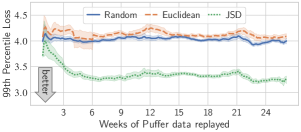
Figure 5. Selecting samples based on the Euclidean distance between batch averages does not improve tail performance. Computing the Jensen-Shanning distance between batch distributions is a better choice.
Mean and 90% CI over a two-week sliding window (see Section 4 for details).

Distribution distances

A natural first choice for batch aggregation is to average sample vectors and compute the Euclidean distance between the averages. However, we find that this approach is flawed: averaging “dilutes” rare values in a batch and the resulting distance is not sensitive to tail differences. Fig. 5 shows that selecting samples based on the Euclidean distance between batch averages does not improve tail performance compared to a random sample selection.

Instead, we aggregate batches by computing an empirical sample distribution. This preserves rare values, but we still need to reduce the dimension to gain any computational benefit from batching. We address this problem using black-box dimensionality reduction (BBDR), an approach inspired by research on dataset shift detection (liptonDetectingCorrectingLabel2018, ) that has been found to outperform alternatives like PCA (rabanserFailingLoudlyEmpirical2019, ). The idea is simple: Use the existing model—trained to identify important feature combinations—to predict $\hat{y}$ (the predicted transmission time), then compute distances in the low-dimensional prediction space. In essence, BBDR leverages prediction as dimensionality reduction tailored to the task at hand.

Finally, we compute the distance between batch distributions using the Jensen-Shannon Distance (JSD) (endresNewMetricProbability2003, ) which is closely related to the Kullback-Leibler Divergence (KL) (kullbackInformationSufficiency1951, ). The KL is an attractive choice to improve tail performance as it puts a large weight on rare values, i.e., values with high probability in one distribution but not in the other. However, the KL has two drawbacks. It is: (i) asymmetric, only sensitive to rare values in one distribution; and (ii) only a divergence, while common density estimation methods require a distance (see below). Thus, we choose the closely related JSD, which is both symmetrical and a distance metric (endresNewMetricProbability2003, ):

Definition 0 (Jensen-Shannon Distance).

Let $P$ and $Q$ be probability distributions, and let $M=\tfrac{1}{2}(P+Q)$. The Jensen-Shannon Distance between $P$ and $Q$ is defined by:

$$JSD(P,Q) =\sqrt{\tfrac{1}{2}\left(KL(P,M)+KL(Q,M)\right)}$$

$$\text{where}\qquad KL(P,M) =\sum_{x\in\mathcal{X}}P(x)\log_{2}\left(\frac{P(x)}{M(x)}\right)$$

if $$P Q \mathcal{X}$$ and are discrete distributions in the space ; or

$$KL(P,M) =\int_{-\infty}^{\infty}p(x)\log_{2}\left(\frac{p(x)}{m(x)}\right)\,dx$$

if $P$ and $Q$ are continuous probability distributions with probability density functions $p$ and $q$, and $m=\tfrac{1}{2}(p+q)$.

Inputs and Outputs

It is not clear a priori whether distances in the sample input or output space are more important for tail performance. Thus, in supervised classification or regression problems—where outputs are available—Memento considers both equally and computes separate distances for both spaces, which are combined below (Section 3.3).

Probabilistic predictions

During batching, Memento leverages probabilistic predictions; e.g., the transition time predictor in Puffer (yanLearningSituRandomized2020, ) outputs a probability distribution over 21 transition time bins. This probability distribution captures whether predictions are somewhat uncertain—thus indicating a need for training using more such samples—or certain. However, we must handle probabilistic estimates differently than point estimates: (i) When batching samples, Memento groups probabilistic predictions first by the distribution mode, then by their probability; (ii) The batch distribution is computed as a mixture distribution, i.e., the prediction distribution for batch $b_{i}$ is $P_{i}(x)=({1}/{|b_{i}|})\cdot\sum P_{j}(x)$, where $P_{j}$ is the probabilistic prediction for sample $j$.

3.3. Density estimation

From the sample distances, we can compute the prediction- and output-space densities. Since we do not know the topology of the sample space, we cannot use simple approximations, such as the fraction of samples per cluster. A common general approach is kernel density estimation (KDE) (parzenEstimationProbabilityDensity1962, ).

Definition 0 (KDE).

Let $b$ be a sample batch and $B$ a set of sample batches, and let $d^{k}(b,\,b^{\prime})=JSD(P^{k},\,{P^{k}}^{\prime})$ with $k\in\{pred,out\}$ be the prediction or output distance between batches $b$ and $b^{\prime}$ with distributions $P^{k},\,{P^{k}}^{\prime}$. Then, using a Gaussian kernel with bandwidth $h$, the kernel density estimate $\hat{\rho}$ at the location of batch $b$ is defined as:

(1) $$\widehat{\rho}_{B}^{\,k}(b)=\frac{1}{\sqrt{2\pi}\,|B|}\sum_{b^{\prime}\in B}\exp\left(-\,\frac{{d^{k}(b,\,b^{\prime})}^{2}}{2h^{2}}\right)$$

Intuitively, the kernel density estimate of $b$ is inversely proportional to the distances to other batches, with diminishing weights for more distant ones. The bandwidth $h$, the “smoothing factor”, determines how quickly this drop-off occurs.

Density aggregation

Memento considers the prediction and output space as equally important. Thus, we aggregate densities using the minimum: we regard the batch as rare if its density is low in either the prediction or output space:

(2) $$\widehat{\rho}_{B}(b)=\min\left(\widehat{\rho}_{B}^{\,pred}(b),\,\widehat{\rho}_{B}^{\,out}(b)\right)$$

If necessary, this approach can be generalized to fewer or more densities: for unsupervised learning without ground truth, Memento can only consider $\widehat{\rho}^{\,pred}$. For models with multiple outputs and thus multiple predictions, we can compute the minimum in Eq. 2 across all respective densities.

Alternative distances

We leverage an information-based distance metric to focus on the tail. However, the density estimation is not tied to this method. Memento is flexible and can operate with any other provided distance metric.

3.4. Sample selection

Memento optimizes the sample-space coverage by iteratively discarding high-density batches. It computes the densities for all samples in $S^{*}=S_{new}\cup S_{mem}$, randomly discards batches with a density-dependent probability (Algorithm 1, Algorithm 1–1) until $|S^{*}|\leq C$, and updates densities after each discard.

Intuitively, Memento assigns a high discard probability to batches with high density—batches for which many similar samples exist—thereby protecting rare low-density samples. However, because noisy samples also seem “rare,” we must retain some probability of discarding rare samples. Memento achieves this by mapping densities to probabilities using softmax with temperature scaling (guoCalibrationModernNeural2017, ):

(3) $$p^{discard}=\operatorname*{soft\,max}\left({\widehat{\rho}_{B}}/{T}\right)$$

where $\widehat{\rho}_{B}$ is a vector of densities for all batches $b\in B$, and $p^{discard}$ is a corresponding vector of discard probabilities.

The temperature $T$ allows balancing tail-focus with noise rejection. A low temperature assigns a higher discard probability to the highest-density batch(es). Conversely, a high temperature assigns more uniform discard probabilities, increasing the probability of discarding low-density batches. At the extreme, the discard probability with $T\to 0$ is a point mass; if Memento is configured with T=0, we thus deterministically discard the highest-density batch. With $T\to\infty$, the probability becomes uniformly random.

3.5. Retraining decision

Intuitively, retraining is beneficial if we collect new information, i.e., samples in areas of the sample space that were previously not covered. That is, we should retrain only when the coverage of sample space increases. Memento’s density estimation allows estimating this increase in information to guide the retraining decision.

Definition 0 (Coverage increase).

Let $B$ be a set of batches with density estimates $\widehat{\rho}_{B}$. We can approximate the region of the sample space covered by the samples in $B$:

(4) $$Coverage(B)=\sum_{b\in B}\widehat{\rho}_{B}(b)$$

Let $B^{\prime}$ be a second set of sample batches. We can approximate the coverage increase, short $CI$, of $B$ with respect to $B^{\prime}$, i.e., the region of sample space covered by $B$ but not by $B^{\prime}$:

(5) $$CI(B,\,B^{\prime})=\sum_{b\in B}\min\left(\widehat{\rho}_{B}(b)-\widehat{\rho}_{B^{\prime}}(b),\,0\right)$$

The relative coverage increase $RCI$ from $B^{\prime}$ to $B$ is then

(6) $$RCI(B,\,B^{\prime})=CI(B,\,B^{\prime})/Coverage(B)$$

where $RCI(B,\,B^{\prime})\in[0,1]$; $0$ means that the same area of sample space is covered, while $1$ indicates that $B$ covers an entirely different region of the sample space than $B^{\prime}$.

Hence, with $B$ the current memory batches and $B^{\prime}$ those used for the last model training, $RCI(B,\,B^{\prime})$ estimates the coverage increase since the last training. If it exceeds the user-defined threshold $\tau$, Memento triggers retraining. This approach presents a rational trade-off: the larger $\tau$, the longer we wait for changes to accumulate before retraining. With a small $\tau$, the model compensates for changes quicker at the cost of more retraining. Memento’s training decision is sample-space-aware, it gives a rational argument that retraining is likely to be beneficial (even if there is no guarantee).

4. Evaluation: Real-world benefits

We use Puffer (Puffer, ) to evaluate Memento’s real-world benefits. This experiment aims to show that Memento improves the tail performance of existing models reliably without significantly impacting the average. Puffer provides both a public dataset with data collected daily over several years and a publicly available model that we can retrain with Memento and compare against the original. This makes Puffer a perfect case study to investigate the following questions:

Q1:

Does Memento improve the tail predictions? Yes
Over years of live and replay data, Memento significantly improves the 1st percentile prediction score.

Q2:

Does it improve the application performance? Yes
On live Puffer, over $10$ stream-years of data, Memento achieves a $14\text{\,}\mathrm{\char 37\relax}$ smaller fraction of stream-time spent stalled with only $0.14\text{\,}\mathrm{\char 37\relax}$ degradation in image quality.

Q3:

Does Memento avoid unnecessary retraining? Yes
Memento retrains 4 times in the first 8 days, and only 3 times in the following 9 months (7 times in total).

Q4:

Are our improvements replicable? Most likely
Memento benefits appear replicable over different time periods of Puffer data. Moreover, its design parameters are intuitive and easy to tune.

Q5:

Can Memento benefit existing solutions? Yes
Memento further improves tail predictions achieved by more advanced training or prediction strategies.

4.1. The Puffer project

The Puffer project is an ongoing experiment comparing ABR algorithms for video streaming (Puffer, ). Puffer streams live TV with a random assignment of ABR algorithms and collects Quality-of-Experience (QoE) metrics: the mean image quality measured in SSIM (zhouwangImageQualityAssessment2004, ) and the time spent with stalled video.

Fugu is the ABR algorithm proposed by Puffer’s authors; it features a classical control loop built around a Transmission Time Predictor (TTP), a neural network predicting the probabilities for a set of discretized transmission times. The TTP was retrained daily with $1\text{\,}\mathrm{M}$ random samples drawn from the past $2$ weeks: $\sim 130\text{\,}\mathrm{k}$ samples from the latest day and $\sim 10\text{\,}\mathrm{\char 37\relax}$ fewer samples for each previous day. Fugu_Feb is a static variant, trained in February 2019 and never retrained.

Fugu was discontinued only $17$ days after Memento’s current deployment. Hence, we can only compare Memento’s long-term performance to Fugu_Feb. As discussed in Section 1, Fugu and Fugu_Feb achieve similar performance: Over almost three years, Fugu showed an SSIM improvement of $0.17\text{\,}\mathrm{\char 37\relax}$ and a reduction in the time spent stalled of $4.17\text{\,}\mathrm{\char 37\relax}$. Thus, improvements over Fugu_Feb would likely translate to similar—yet slightly lesser—improvements over the daily-retrained Fugu.

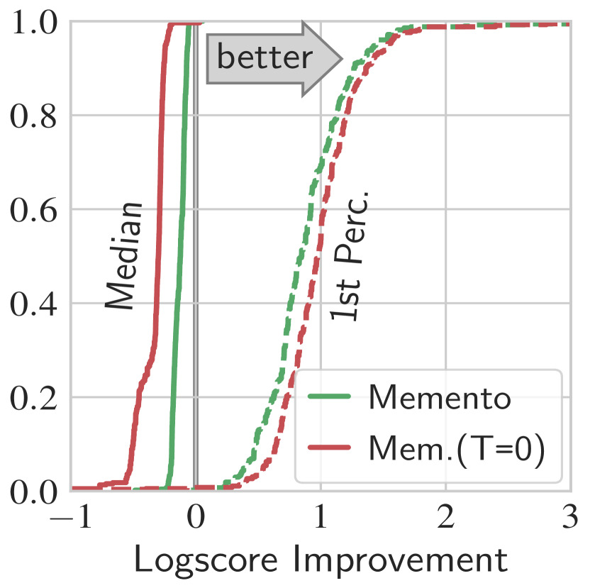
(a) Memento improves the prediction quality at the tail, with a relatively small impact on the median prediction quality.

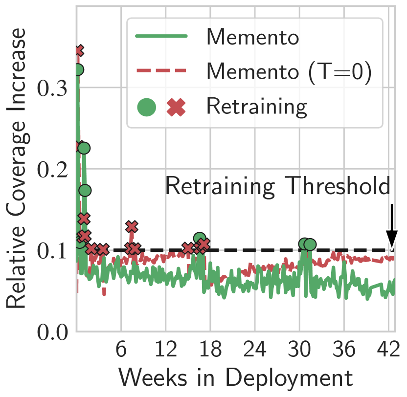
(b) Memento avoids unnecessary retraining. Its deterministic variant ($T=0$) is less efficient and does not converge.

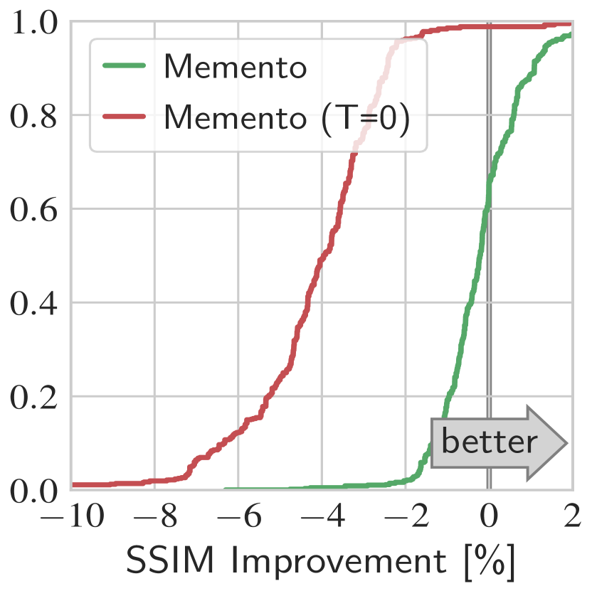
(c) Memento degrades the SSIM slightly ($0.14\text{\,}\mathrm{\char 37\relax}$ worse). The det. variant degrades it notably ($4.4\text{\,}\mathrm{\char 37\relax}$ worse).

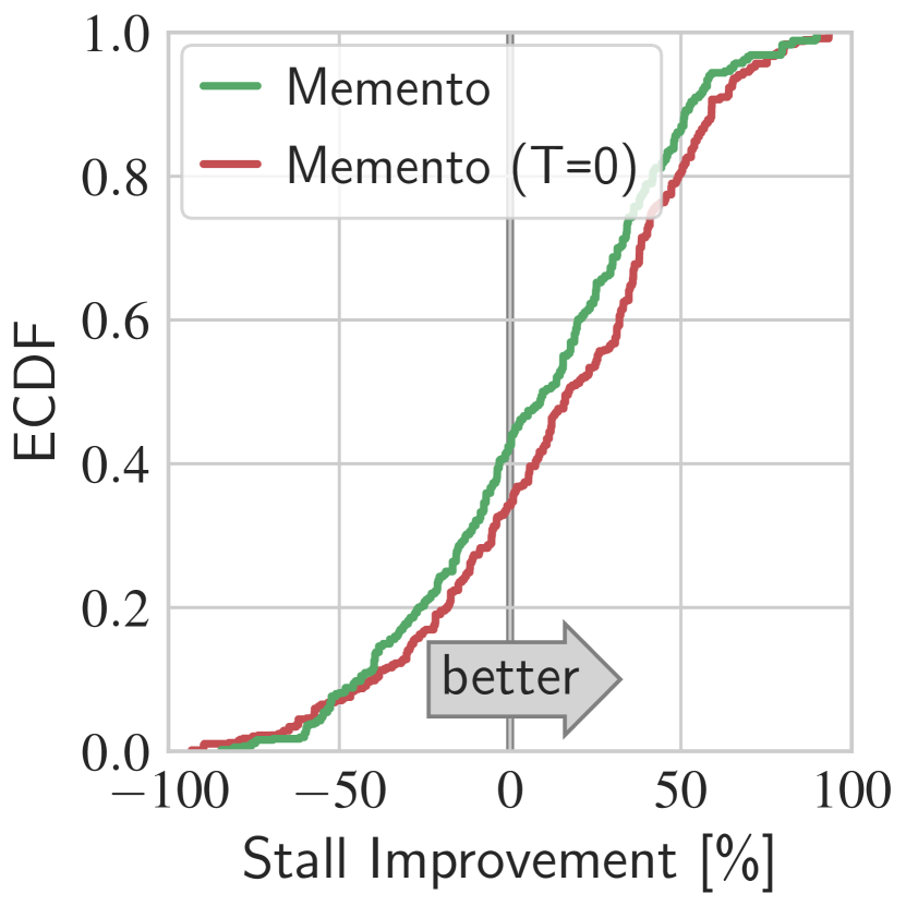
(d) Memento reduces the fraction of stream-time spent stalled by $14\text{\,}\mathrm{\char 37\relax}$, although results vary by day.

Figure 6. Memento achieves its goal: it improves the tail prediction quality with minimal impact on the average (Fig. 6(a)). This requires little retraining (Fig. 6(b)) and translates into notable QoE improvements (Figs. 6(c) and 6(d)).

4.2. Retraining with Memento

We use Memento to retrain Fugu’s TTP: every day, we use Memento to select the training samples and decide whether to retrain. We assess Memento’s benefits in two experiments:

Deployment:

We deploy on Puffer two Memento variants, i.e., two variants of Fugu using Memento for retraining the TTP. One uses Memento’s default parameters (see below), and the other deterministic sample selection (i.e., using temperature $T=0$, Section 3.4). We collected data over $292$ days (from Oct. 2022 to Jul. 2023), totaling around $10.8$ stream-years of video data per variant. This experiment allows answering Q1, Q2, and Q3.

Replay:

To confirm the deployment observations, evaluate design choices, and benchmark the impact of Memento’s parameters, we replay Puffer data collected since 2021. To reduce the bias from a particular starting day, we replay $3$ instances with $6$ months of video data each and a total of $90$ stream-years of video data. This experiment allows answering Q4 and Q5.

Metrics

We access Memento along three dimensions:

• Prediction quality is measured with the logarithmic score ${logscore(y)=\log p(y)}$ (gneitingStrictlyProperScoring2007, ); $y$ is the video chunk transmission time and $p(y)$ the TTP-predicted probability. Score improvement equals TTP loss decrease. Available in deployment and replay.

• Application performance is measured with user QoE; Only available for the deployment experiment, where real user streams are impacted by the predictions and the resulting QoE can be measured.

• Training resource utilization is measured by the number of retraining events in deployment and replay.

Parameters

We set Memento’s memory capacity $C$ to $1\text{\,}\mathrm{M}$ samples (same as the original Fugu model). Default parameters are a retraining threshold $\tau$ of $0.1$, batching size $b$ of $256$, kernel bandwidth $h$ of $0.1$, and temperature $T$ of $0.01$. We evaluate the impact of different parameter values in Section 4.4.

4.3. Deployment results

In this section, we show that Memento effectively improves the tail prediction quality with little retraining and that this translates into QoE improvements over Fugu_Feb.

In Appendix B, we provide additional plots with the evolution of QoE and predictions over time, and aggregate plots like those published on the Puffer paper and website (yanLearningSituRandomized2020, ; Puffer, ).

Prediction quality

Fig. 6(a) shows the score difference ECFD between Memento and Fugu_Feb in median and 1st-percentile scores on the whole deployment (higher is better).

We observe that Memento improves tail predicition performance as intended, with a slight—yet expected—degradation on average: as memory is finite and Memento purposefully prioritizes “rare” samples, it must remove samples for the most common cases. The deterministic version of Memento prioritizes the tail more aggressively, which leads to slightly better tail improvements and worse median degradation.

Retraining count

Fig. 6(b) shows the relative coverage increase $RCI$ between the current memory and the one last used to retrain the model, as well as the retraining threshold $\tau=0.1$. We observe about eight “warm-up” days where Memento retrains four times. Afterward, RCI remains low and retraining due to changes in the data (RCI peaks) happens three times. This shows that there are fewer “new patterns” to learn from over time; retraining daily is unnecessary.

Conversely, the deterministic variant of Memento keeps accumulating samples, exhibiting a different RCI pattern. After training five times during “warm-up,” it trained $9$ more times. Where RCI for default Memento stabilizes, the RCI of the deterministic variant slowly but steadily increases over time while it accumulates rarer and rarer samples, as it does not reject noise. Essentially, this variant “never forgets.”

Application performance

Figs. 6(c) and 6(d) show the relative QoE improvements achieved over Fugu_Feb for the SSIM and the time stalled (higher is better), respectively.

First, we observe that Memento only marginally affects the SSIM; the average SSIM is $17.12$ and $17.14$ for Memento and Fugu_Feb, resp. (not shown). Memento’s deterministic variant affects the SSIM more; its average is $16.39$ (not shown) and the SSIM is consistently worse than Fugu_Feb (Fig. 6(c)).

Second, Fig. 6(d) shows that the improvement in stalls compared to Fugu_Feb is almost the same for both variants of Memento, even though there are large day-to-day variations: some days, Fugu_Feb stalls much less than Memento, and vice versa. Over the entire $292$ days of deployment, Memento spent a fraction of $0.2\text{\,}\mathrm{\char 37\relax}$ of stream-time stalled, compared to $0.24\text{\,}\mathrm{\char 37\relax}$ for Fugu_Feb. In relative terms, Memento spent a $14\text{\,}\mathrm{\char 37\relax}$ smaller fraction of stream time stalled than Fugu_Feb.

In the results above, we already see that Memento performs slightly worse without noise rejection (i.e., with $T=0$). In a previous deployment, we observed that never forgetting ultimately prevented enough average samples from remaining in memory, which destroyed the average performance (Appendix B). The latest version of Memento made the deterministic variant more robust but we see the signs of noise accumulation (worse predictive performance, more frequent retraining, steadily rising RCI). By contrast, the probabilistic default Memento naturally forgets noise and stabilizes, as can be seen in the RCI in Fig. 6(b).

Finally, we observe that Memento reduces stalls by $3.5$ times as much as retraining daily with random samples. In Appendix B, Fig. 14 we show Fig. 6(a) overlaid with the score improvements of Fugu in the past. We observe that random retraining improved the tail prediction scores significantly less and even worsened them on $20\text{\,}\mathrm{\char 37\relax}$ of days.

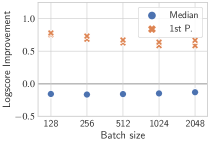
(a) Larger batches slightly degrade the tail with no impact on the median.

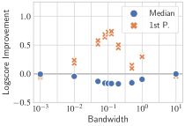
(b) A kernel bandwidth around $0.1$ is best. Extreme values nullify benefits.

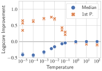
(c) $T=0.01$ is a good trade-off between tail prioritization and randomness.

Figure 7. Each marker shows the median prediction improvement of Memento over Fugu (random selection) over a $6$-month replay, measured as median and 1st perc. improvement each day. Results are consistent across replays.

From predictions to QoE

One may wonder why the average prediction degradation (Fig. 6(a)) does not seem to strongly impact image quality (Fig. 6(c)), and, conversely, why significant tail improvements yield only a modest reduction in stalls (Fig. 6(d)). Our results illustrate the complex relationship between predictions and QoE, including the closed-loop control logic, which uses the predictions and aims to keep the video buffer at the receiver sufficiently full to avoid stalling.

Looking closer, we noticed that the transmission time of most chunks is very small, and most prediction errors are also small time-wise. Hence, slightly worse predictions have little effect on the buffer fill level; the controller has time to compensate and maintain image quality. Moreover, since most prediction errors overestimate the transmission time (not shown), it makes the closed-loop control more conservative. Thus, it manages to keep stalls low but struggles to maintain high image quality (compare Figs. 6(c) and 6(d)). Further investigations of the interplay between prediction quality and application performance would be interesting but are beyond the scope of this work. To facilitate further research, we publish all our retrained models including their training sample selection alongside the Puffer QoE data.

4.4. Replay results

In this section, we confirm that Memento’s benefits are replicable and not just an artifact from deploying at an “easy time,” its design decisions are justified, and it complements existing techniques. To do this, we replay $3$ non-overlapping instances of $6$ months with $253926$ stream-years of video-data respectively and $3\text{\,}\mathrm{M}$ samples on average per day.

To monitor the memory quality over time, we disable threshold-based retraining and retrain every $7$ days; one must retrain and test the model to assess whether the right samples were selected. We evaluate each day in terms of prediction improvement over retraining with random samples (Fugu) and report the mean over each $6$-month period. We show the entire time series for each experiment in  Appendix B.

Replicability

All plots in Fig. 7 show three data points per setting, which are average performance numbers over the entire $6$ month period. We observe that all results are fairly stable, which gives reasonable confidence about the replicability of Memento’s benefits on this use case.

Batch size

Fig. 7(a) shows Memento’s prediction performance over the batch size; larger sizes improve scalability but make sample selection more coarse-grained, which should hurt performance (Section 3.2). We observe a slight tail performance drop for larger batch sizes with little change on average.

Regarding scalability, differences are more pronounced: using a single CPU core to process $4\text{\,}\mathrm{M}$ samples takes on average $200\text{\,}\mathrm{s}$ with a batch size of $128$, $48\text{\,}\mathrm{s}$ with $256$ (the default), and $7\text{\,}\mathrm{s}$ with $1024$. Benefits flatten out for larger batch sizes. Overall, computation is dominated by distance computation; batching the samples takes only about $2.5\text{\,}\mathrm{s}$.

Bandwidth

For each batch, Memento estimates how close nearby batches are; the kernel bandwidth $h$ determines what “nearby” means (Section 3.3). As the computed distances $JSD(P,Q)\in[0,1]$, bandwidths $>1$ over-smooth (all batches are always “nearby”), and bandwidths $\ll 1$ under-smooth (no other batches are ever “nearby”). Both cases nullify the idea of estimating density, effectively making the sample selection random. Fig. 7(b) confirms this intuition: at the extremes, Memento performs like a random selection. We obtain the best tail improvement with a bandwidth around $1\text{\times}{10}^{-1}$.

Temperature

Fig. 7(c) shows Memento’s prediction performance over the temperature $T$; a low temperature strongly prioritizes rare samples at the risk of accumulating noise, while a high temperature rejects noise by making the sample selection more random (Section 3.4). As expected, a lower temperature yields better tail performance but degrades the average. The trade-off is not linear, though; we can select a temperature that provides tail benefits with minimal impact on the average. The best trade-off is a temperature around $1\text{\times}{10}^{-2}$.

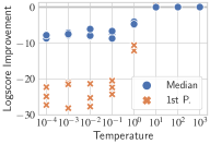
Figure 8. Loss-based selection is worse and less robust.

Alternative selection metrics

Fig. 8 shows the performance of using loss as an alternative selection metric: we still use temperature-based probabilistic selection but prefer to discard samples with a low loss rather than high density. At best, it gives tail improvements about half as Memento, but it is much harder to tune: the benefits vanish for a slightly higher temperature. With a lower temperature, i.e., selecting more strongly based on loss, the model performance decreases drastically, which mirrors our observations in Section 2.

We evaluate additional metrics in Appendix B: prediction confidence, label counts, and whether a sample belongs to a stalled session or not. In summary, these perform worse or equal to loss-based selection in the best case, and most of them are as sensitive to tune. Probabilistic selection based on density performs better and is less sensitive (see Fig. 7(c)). We also show detailed results for Euclidean distances (Section 3.2).

Alternative training decision

We compare Memento’s retraining decision based on the relative coverage increase RCI with a loss-based decision (not shown). We observe that for samples selected by Memento, either decision is effective. Overall, a coverage-based decision provides greater control over retraining frequency but struggles with low thresholds (e.g., $5\text{\,}\mathrm{\char 37\relax}$). As Memento is probabilistic, the estimated RCI fluctuates at each iteration, which can be observed in Fig. 6(b), and the retraining threshold should be set above these fluctuations. It may be possible to further improve Memento by smoothing the RCI or by attempting to remove the random fluctuations. We leave this challenge for future work.

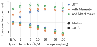
Figure 9. Memento complements training and prediction improvements such as JTT and Matchmaker.

Memento $+$ Matchmaker $+$ JTT

MatchMaker (mallickMatchmakerDataDrift2022, ) improves predictions by using an ensemble of models (default is $7$) combined with an online algorithm to select the best model to make a prediction for each sample. However, this is limited by the performance of the individual models. Using an ensemble of models trained with a random selection, even with an oracle choosing the best model, we can only improve tail performance by half as much as a single model trained with Memento. However, we can get the best of both worlds by using MatchMaker with an ensemble of Memento-trained models, which yields double the tail performance with less decrease in median performance compared to a single Memento-trained model (‘no upsampling’ in Fig. 9).

JTT (liuJustTrainTwice2021, ) improves performance by training twice: after the first training, misclassified samples are upsampled in the second and final training. Fig. 9 shows the same performance tradeoffs for JTT and Memento: both improve the tail and degrade the median: JTT with an upsampling factor of $3$ is roughly equivalent to Memento’s sample selection with ‘normal’ training. Yet this comes at different resource costs: JTT requires up to double the training time and resources, depending on how long the first training step is. Training models like Puffer takes time in the range of hours (yanLearningSituRandomized2020, ) and often requires expensive hardware (e.g., GPUs). Memento is more resource efficient: even on a single CPU core, it can process millions of samples in a few minutes (see above). However, JTT and Memento are not in competition, but complementary. We observe the best performance by combining Memento-selected samples with JTT’s training and observe even further improvements when the resulting models are used in a MatchMaker ensemble for predictions (Fig. 9).

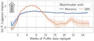
Figure 10. Over time, Memento outperforms QBC.

Query-by-Committee

A Memento-trained ensemble not only outperforms an ensemble trained with random samples but also an ensemble trained with the Query-by-Committee (QBC) algorithm (seungQueryCommittee1992, ) (Fig. 10). QBC selects samples with the highest prediction entropy between all members of the ensemble. In theory, these samples contain the most information for learning. We repeat the MatchMaker-Oracle experiment and compare an ensemble of Memento-trained models with an ensemble of QBC-trained models.

Fig. 10 shows that the tail improvements of QBC initially exceed Memento, and are comparable to Memento with JTT (Fig. 9). However, the QBC ensemble degrades over time and ultimately settles on less than a third of Memento’s improvement. We suspect this comes from QBC accumulating noise. Both Memento and QBC initially pick up noise (low density; high entropy). Memento’s probabilistic approach prevents noise from accumulating (Section 3.4) while QBC degrades: selecting noise biases the model toward random predictions, increasing the prediction entropy of any sample, thus decreasing QBC’s ability to identify informative samples.

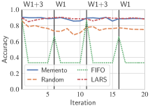
(a) Rare and infrequent traffic patterns: Only LARS and Memento avoid forgetting. Traffic for W2 is always present; for W1 and W3 only where marked.

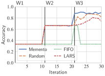
(b) Incremental learning: Memento efficiently integrates workload traffic patterns as they appear sequentially where marked, replacing the previous ones.

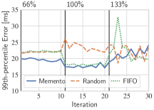
(c) Increasing congestion: Memento has comparable or lower 99th percentile error for the marked level of network utilization,i.e., increasing congestion.

Figure 11. Memento can handle various traffic patterns and prediction types, outperforming other approaches.

5. Evaluation: Synthetic shifts

In the previous section, we showed that Memento provides significant benefits in a real-world use case. In this section, we use ns-3 (rileyNs3NetworkSimulator2010, ) simulations of data center workloads to show that sample selection with Memento applies to other settings as well. Specifically, we show that Memento:

1. ensures good tail performance by reliably prioritizing samples from infrequent traffic patterns (Section 5.2);

2. picks up new patterns quickly (Section 5.3);

3. is applicable to classification and regression (Section 5.4).

5.1. Experimental setup

Sample selection strategies

We compare Memento with two baselines: Random (random sampling) and FIFO (keep recent samples). In addition, we compare it to the state-of-the-art LARS (Loss-Aware Reservoir Sampling, (buzzegaRethinkingExperienceReplay2020, )). LARS uses several improvements to random sampling for classification, and has two stages: first, it randomly chooses to keep or discard a new sample, with probability exponentially decreasing over time; second, it considers both label counts and loss to decide which in-memory sample to replace.

Parameters

For Memento, we use the same default parameters as before: a batching size of $256$, kernel bandwidth $h$ of $0.1$, and temperature $T$ of $0.01$. We reduce the memory capacity $C$ to $20\text{\,}\mathrm{k}$ samples (i.e., $1$/$50$ compared to Section 4) for two reasons: (i) We aim to show the limitations of different sample selection strategies, which is easier to do using small memories; (ii) LARS scales poorly, making comparing performance on larger memory sizes impractical—we optimized the original LARS implementation to scale to $20\text{\,}\mathrm{k}$ samples. Our optimization is available in our artifacts.

Workloads

The simulation setup (Appendix C, Fig. 15) consists of two nodes and applications sending messages whose sizes follow three empirical traffic distributions from the Homa project (Fig. 16, (montazeriHomaReceiverdrivenLowlatency2018, )): Facebook web server (W1), DC-TCP (W2), and Facebook Hadoop (W3). W1 and W3 are similar size-wise, while W2 messages are about an order of magnitude smaller. For each workload, we generate $20$ traffic traces of $1\text{\,}\mathrm{min}$ each. During this time several senders transmit a combined $20\text{\,}\mathrm{M}\mathrm{b}\mathrm{p}\mathrm{s}$, resulting in an average network utilization of $66\text{\,}\mathrm{\char 37\relax}$. We repeat this process by injecting additional cross traffic to reach an average utilization of $100\text{\,}\mathrm{\char 37\relax}$ and $133\text{\,}\mathrm{\char 37\relax}$, respectively. We use different random initializations to generate a total of 180 distinct runs that we combine in various iterations in the following experiments.

Models

We compare the selection strategies for two neural networks; one for classification and one for regression. The classification model predicts the application workload: Each input is a trace of the past $128$ application packet sizes, and the model predicts the probabilities for each workload. The regression model predicts the next transmission time from past packets: Each input contains a trace of the past $127$ packet sizes and transmission times, the current packet size, and the model predicts the transmission time. See Appendix C for architecture and hyperparameter details.

Metrics

For classification tasks, we measure the balanced accuracy, i.e., the accuracy obtained over an equal number of evaluation samples per workload, ensuring equal importance of each workload. In other words, performance is evaluated over an equal distribution of overall workloads, regardless of whether they are present at the current iteration. Good performance requires both picking up new patterns quickly and avoiding catastrophic forgetting.

For regression, we investigate changes in traffic distribution (see below) and measure the 99th percentile absolute prediction error over the data in the latest iteration. Good performance requires picking up new patterns quickly.

5.2. Classification: Rare patterns

In the first experiment, we show that Memento successfully picks up samples from infrequent traffic patterns. To do so, we use highly imbalanced traffic: W1 and W3 only constitute $\leq 2\text{\,}\mathrm{\char 37\relax}$ of overall traffic. Good tail performance implies high accuracy not only for W2 but also for W1 & W3.

Setup

We use the classification model and iterate over samples from $20$ runs. We use W2 at every iteration, representing a large part of traffic that remains relatively unchanged. On top of that, we include W1 once every five iterations, and W3 once every ten iterations; they represent sporadic traffic patterns that make up for $1.30.5\text{\,}\mathrm{\char 37\relax}$ of traffic respectively.

Results

Memento and LARS retain sufficient samples from each workload and show the best accuracy over all iterations (Fig. 11(a)). On the other hand, FIFO shows good accuracy only while all workloads are present, as the large number of samples of W2 quickly overwrites W1 & W3 otherwise. While Random achieves better results than FIFO, it ultimately retains too few samples of W1 & W3, as they make of less than $2\text{\,}\mathrm{\char 37\relax}$ of samples in memory.

5.3. Classification: Incremental learning

Next, we show that Memento quickly picks up new patterns and avoids catastrophic forgetting in an ‘Incremental Learning’ setting, which is known for its challenging nature (farquharRobustEvaluationsContinual2019, ).

Setup

We use the same model and setup as Section 5.2, but iterate over samples from each workload sequentially; first W1, then W2, and finally W3, for $10$ iterations each.

Results

We find that overall, Memento exhibits the best performance. Both Random and LARS struggle because of their sample selection rate (Fig. 11(b)); these two flavors of random memory avoid forgetting by decreasing the probability of selecting new samples over time. When W3 is introduced, they are slow to incorporate new samples (Appendix C, Table 2). While both LARS and Random are slow to react, the fact that the balanced accuracy of LARS is worse than Random’s is mostly an artifact of the similarity of W1 and W3: LARS has (desirably) retained more samples of W1, yet this causes its model to mistake W3 for W1 more often than Random, which has forgotten most of W1 and is consequently less biased. By manually tuning the sampling rate of LARS to be much more aggressive, we were able to achieve the same performance as Memento (not shown). This highlights the benefit of the self-adapting nature of Memento’s sample-space-aware approach: If a new label appears, Memento discovers that this part of the sample space is not well covered yet. It quickly prioritizes discarding common in-memory samples to retain samples from the new label.

5.4. Regression

In this experiment, we show that Memento is applicable to regression and handles complex traffic changes. We iterate from $66$ to $133\text{\,}\mathrm{\char 37\relax}$ network utilization, which presents more complex gradual changes in traffic patterns than the abrupt changes in workload distributions (Sections 5.3 and 5.2).

Setup

We iterate over traffic from all workloads using runs with increasing congestion. For the first $10$ iterations, we use runs with $66\text{\,}\mathrm{\char 37\relax}$ network utilization, followed by $10$ iterations of $100\text{\,}\mathrm{\char 37\relax}$, and finally $10$ iterations of $133\text{\,}\mathrm{\char 37\relax}$. We report the 99th percentile error under the current traffic conditions.

Results

Memento generally shows the lowest 99th percentile prediction error (Fig. 11(c)). Random is slow to react to the new patterns and requires several iterations to adjust to the new traffic conditions. Perhaps surprisingly, FIFO performs well up to $100\text{\,}\mathrm{\char 37\relax}$ utilization but shows very unstable performance for $133\text{\,}\mathrm{\char 37\relax}$. LARS is not applicable to regression.

6. Related work & Discussion

Limitations

Let us address the elephant in the room: Memento cannot do anything with a bad model or dataset. It helps identify the most useful samples for training, but those samples must be present in the dataset in the first place, and the model must be capable of learning from them.

We find that density-based selection performs well but is probably not optimal. It addresses the problem of dataset imbalance well, but it is less effective to differentiate “hard-to-learn” from “easy-to-learn” samples, which is better captured by the model loss. Combining both would likely be beneficial.

Finally, density computations limit Memento’s scalability. Batching helps (Fig. 5), but it would not be enough to process data streams with billions of samples per day.

Continual learning

Continual learning and dataset imbalance correction are well-studied problems. Fundamentally, continual learning suffers from the stability-plasticity dilemma (ditzlerLearningNonstationaryEnvironments2015, ): a stable memory consolidates existing information yet fails to adapt to changes, while a plastic memory readily integrates new information at the cost of forgetting old information. Forgetting old-yet-still-useful information is known as catastrophic forgetting (mcclellandWhyThereAre1995, ). Continual learning approaches aim to be as plastic as possible while minimizing catastrophic forgetting. They can be broadly categorized as either prior-based or rehearsal-based (buzzegaRethinkingExperienceReplay2020, ). Prior-based methods aim to prevent catastrophic forgetting by protecting model parameters from later updates (kirkpatrickOvercomingCatastrophicForgetting2017, ; parisiContinualLifelongLearning2019, ; zenkeContinualLearningSynaptic2017, ). Rehearsal-based methods collect samples over time in a replay memory and aim to prevent forgetting by learning from both new and replayed old data (buzzegaRethinkingExperienceReplay2020, ; iseleSelectiveExperienceReplay2018, ; ratcliffConnectionistModelsRecognition1990, ). Hybrid methods combine both, e.g., training with a replay memory and a loss term penalizing performance degradation on old samples (rolnickExperienceReplayContinual2019, ).

Memento builds on previous rehearsal-based approaches, incorporating ideas such as coverage maximization (debruinImprovedDeepReinforcement2016, ). It extends existing ideas by considering both prediction and output spaces, leveraging temperature scaling to control the tail-focus and introducing a novel coverage increase criterion to reason about when to retrain. Similar to Memento, Arzani et al. (arzaniInterpretableFeedbackAutoML2021, ) also suggest using the “right samples” to retrain AutoML systems (heAutoMLSurveyStateoftheart2021, ): They use the disagreement among a set of models to identify “the tail” and guide the user to collect more tail samples and add them to the training set. However, this does not apply to all networking applications; e.g., we cannot “force” streaming sessions to come from rare network paths or experience particular congestion patterns over the Internet; we must do with the available samples.

Distribution shift detection

Continual learning closely relates to a branch of research aiming to keep models up-to-date upon changes in the data-generating process—known as distribution shifts. State-of-the-art methods rely on statistical hypothesis testing (hinderNonParametricDriftDetection2020, ) or changes in empirical loss (tahmasbiDriftSurfStableStateReactiveState2021, ), plus a time-based window (or multiple parallel windows) (ditzlerLearningNonstationaryEnvironments2015, ). When a change is detected, these algorithms advance the time window(s), discard “outdated” samples whose timestamp falls outside of the window(s), and retrain.

Shift detection algorithms make sample-space-aware retraining decisions but lack a comparable selection strategy. Once a change is detected, they discard all old samples. This approach is too coarse-grained for networking: Network traffic is composed of many patterns (Appendix B, Fig. 12) and not all patterns get outdated at once.

Matchmaker (mallickMatchmakerDataDrift2022, ) proposes a more incremental approach to shifts in networking data. It uses an ensemble of models and “matches” each sample to the model trained with the most similar data. However, it does not address the sample selection problem: If no model in the ensemble is good at the tail, matching will not help. By contrast, Memento builds upon ideas originating from shift detection (BBDR (liptonDetectingCorrectingLabel2018, )) and extends the sample-space-aware strategy to the sample selection to train better models. Our evaluation shows that a single Memento-trained can outperform Matchmaker at the tail, even if using an oracle to match the optimal model (Section 4.4).

Experience replay for reinforcement learning

While we evaluate Memento in the context of supervised learning, it may also be used for reinforcement learning (RL), which is popular approach to ML-based ABR (xiaGenetAutomaticCurriculum2022, ; maoNeuralAdaptiveVideo2017, ). In fact, RL commonly uses a replay memory (vanhasseltDeepReinforcementLearning2016, ; riedmillerNeuralFittedIteration2005, ), and it has been shown that it can greatly improve RL performance (aljundiOnlineContinualLearning2019, ; rolnickExperienceReplayContinual2019, ).

Transformers and other large models

In recent years, large models with billions of parameters have become popular in natural language processing (devlinBERTPretrainingDeep2019, ; openaiGPT4TechnicalReport2023, ; touvronLlamaOpenFoundation2023, ) and computer vision (hanSurveyVisionTransformer2022, ; khanTransformersVisionSurvey2021, ), usually based on Transformer architectures (vaswaniAttentionAllYou2017, ); there are also first trials in networking (dietmullerNewHopeNetwork2022, ; leRethinkingDatadrivenNetworking2022a, ; mondalWhatLLMsNeed2023, ).

We have evaluated Memento primarily on small models to investigate to impact of a smarter sample selection instead of using more resources such as more complex models and cannot claim with confidence that we would see comparable improvements for them. However, there is mounting evidence that even large transformer models suffer from data bias (birhaneLAIONsInvestigatingHate2023, ; longprePretrainerGuideTraining2023, ; zhaoUnderstandingEvaluatingRacial2021, ), which Memento may help to address.

Furthermore, an important part of these models is an encoder that translates text, images, or other data into a latent space. Latent space representations have seen use in clustering (mukherjeeClusterGANLatentSpace2019, ), and Memento may benefit from computing sample distances in this latent space, similar to how it uses BBDR.

Data processing

Data validation and augmentation are important steps of any ML pipeline. Especially in ML systems that are evolving over time, new bugs may be introduced any time the model or data collecting system are updated. These bugs may lead to erroneous data, and data validation is necessary to prevent such data from becoming part of the training data (polyzotisDataValidationMachine2019, ). Furthermore, collected data is often augmented to address dataset imbalance by generating additional synthetic samples or upscaling existing ones, which can improve performance and reduce overfitting (wongUnderstandingDataAugmentation2016, ). One example is Just Train Twice (JTT) (liuJustTrainTwice2021, ), which trains a model, uses it to identify misclassified samples, upsamples those, and trains again. As a replay memory, Memento operates between the validation and augmentation steps, and complements them. For example, we showed in Section 4.4 that JTT’s upsampling is more effective when Memento has identified tail samples first. Only validated data should be considered by the sample selection, and selected samples may be augmented. In particular, the memory should only store non-augmented samples, as augmenting the data before passing it to the memory can result in the sample selection to overfit to the augmentation (buzzegaRethinkingExperienceReplay2020, ).

Generalization

Memento could be applied to other ML-based networking applications, including congestion control (abbaslooClassicMeetsModern2020, ; jayDeepReinforcementLearning2019, ; nieDynamicTCPInitial2019, ; winsteinTCPExMachina2013, ), traffic optimization (chenAuTOScalingDeep2018, ), routing (valadarskyLearningRoute2017, ), flow size prediction (dukicAdvanceKnowledgeFlow2019, ; poupartOnlineFlowSize2016, ), MAC protocol optimization (jogOneProtocolRule2021, ; yuDeepReinforcementLearningMultiple2019, ), traffic classification (busse-grawitzPForestInNetworkInference2019, ; wichtlhuberIXPScrubberLearning2022, ), network simulation (zhangMimicNetFastPerformance2021, ), or DDoS detection (wichtlhuberIXPScrubberLearning2022, ). Networking has proven to be a challenging environment for ML, and many proposed systems have only delivered modest or inconsistent improvements in real networks (yanLearningSituRandomized2020, ; bakshyRealworldVideoAdaptation2019, ; bartulovicBiasesDataDrivenNetworking2017, ; yanPantheonTrainingGround2018, ). In response, research has focused on providing better model architectures (abbaslooClassicMeetsModern2020, ; jayDeepReinforcementLearning2019, ; yanLearningSituRandomized2020, ) and training algorithms (xiaGenetAutomaticCurriculum2022, ), model ensembles for predictions and active learning (mallickMatchmakerDataDrift2022, ; heAutoMLSurveyStateoftheart2021, ), real-world evaluation platforms (yanPantheonTrainingGround2018, ; yanLearningSituRandomized2020, ), uncertainty estimation (rotmanOnlineSafetyAssurance2020, ) and model verification (eliyahuVerifyingLearningaugmentedSystems2021, ).

A better sample selection is beneficial to all these advances. Memento is orthogonal to and complements these works, opening an exciting potential. We show in Section 4.4 that combining Memento with JTT or Matchmaker improves performance further: once Memento decides to retrain, we train better with JTT, and MatchMaker benefits from an ensemble of Memento-trained models. However, optimizing training or model architectures is beyond the scope of this work, which focuses on identifying the most valuable samples for retraining and deciding when to retrain. We look forward to future research investigating, e.g., how to design ML models to best leverage coverage maximization.

Ethical issues

This work does not raise any ethical issues.

Appendix A Artefacts and Replication.

All code to reproduce the results in this paper is publicly available and provided as an archive in the supplemental material of this paper for review. The archive contains a README with specific instructions on how to run the code. Below, we give an overview of reproducing the Puffer and synthetic results, and how to use Memento in other projects.

Puffer

All Puffer-based experiments are based on the data published by the Puffer project (Puffer, ). To replicate our results, you need to first download the Puffer data with the commands provided in the README file. It is possible to download only a subset of the published data to save both space and computation time. In particular, we provide a small demonstration script that uses the same code as our main experiments but uses a week of data.

Once data is downloaded, you can run two kinds of commands, both of which are described in the README file: analysis and replay. The analysis aggregates the downloaded data to create the figures shown in Section 4.3, comparing the performance of Memento to Fugu. The replay retrains the TTP model with data selected by Memento to create the figures shown in Section 4.4, evaluating different parameter choices with different periods of data to ensure that results are replicable.

Synthetic

All synthetic experiments are based on data generated by an ns-3 network simulation. We provide the data used in the paper as well as the simulation scripts to (re-)generate it. The README file describes the commands to replay the simulation data for retraining with Memento to create the figures shown in Section 5.

Memento

We provide the implementation of Memento as a Python package so it can be easily included in other projects. Our implementation offers a clean interface for instantiating a memory with a given capacity, which exposes methods to insert and get samples. We provide implementations for the distance metrics used in this paper, as well as a generic interface to implement new metrics. Finally, we also implement alternative sample selection strategies with the same interface, such as random selection, loss-based selection, or LARS (see Section 5), as well as an interface to combine multiple memories.

Appendix B Puffer: Supplemental Results

Recurring patterns

Fig. 12 illustrates that the Puffer traffic does contain patterns that recur at the tail. Each line in this plot corresponds to one batch in the memory assembled by Memento after three weeks of sample selection. The lines show the density of batches with respect to the daily samples over the next 200 days; this captures “how similar the batches in memory are to the traffic of the current day.” It shows that some tail batches (the lines with the lowest densities) are sometimes more represented in the daily traffic for a couple of days (see e.g., the step around week 7), then fade away.

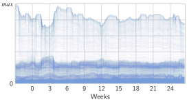
Figure 12. Coverage of batches in the daily samples

Aggregate performance

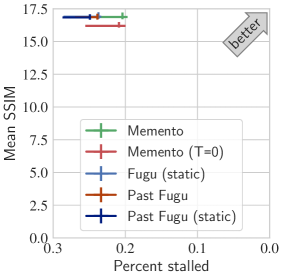
(a) Image quality and fraction of stream-time spent stalled.

(b) Zoomed in.

Figure 17. Aggregate performance. Mean and bootstrapped 90% confidence intervals from the deployment of the current version of Memento on September 19th, 2022 until February 13th, 2023. ABRs annotated with ‘past’ indicate past data from April 9th, 2020 until October 5th, 2022, when Fugu was discontinued.

Fig. 17 shows the aggregated SSIM and percent of stream-time spent stalled on a 2D grid in the style of the Puffer (yanLearningSituRandomized2020, ) publication and website (Puffer, ). Concretely, we show two sets of ABRs. First Memento (default and $T=0$) and Fugu_Feb, aggregated since the latest version of Memento was deployed on September 19th, 2022 until February 13th, the cutoff for our current evaluation. We cannot aggregate over the deployment duration Fugu as it was discontinued on October 5th. Thus, we additionally include a second set consisting of Fugu and Fugu_Feb, aggregated from 2020 until Fugu was discontinued.

Timeseries (real-world)

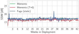
(a) Image quality, measured in SSIM.

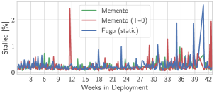
(b) Percent of stream-time spent stalled.

Figure 18. Evolution of QoE metrics over time. Absolute Values for each ABR.

Fig. 18 shows QoE results per day over time for Memento with default parameters, Memento ($T=0$) and for Fugu_Feb since September 19th.

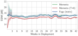
(a) Image quality, measured in SSIM.

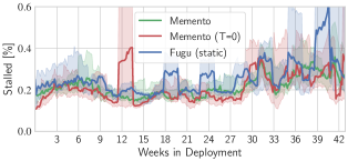
(b) Percent of stream-time spent stalled.

Figure 19. Evolution of QoE metrics over time. Absolute Values for each ABR. Mean and bootstrapped 90% confidence interval over two-week sliding windows.

Fig. 19 shows the same results, but the mean and bootstrapped 90% CI over a two-week sliding window.

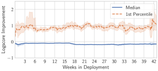
(a) Memento.

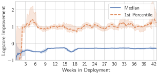
(b) Memento ($T=0$).

Figure 20. Logscore improvements compared to Fugu_Feb.

Fig. 20 shows the prediction improvements over Fugu_Feb for Memento with default parameters and with $T=0$.

Past degradation of Memento ($T=0$) over time

In a previous deployment, we observed Memento ($T=0$) to degrade over time, as shown in Fig. 13. Without forgetting, it kept accumulating noise and retraining. At first, the Puffer control loop around the TTP was able to compensate for this degradation, but as the model became too bad, it failed. Over time, the Image quality degraded by over $30\text{\,}\mathrm{\char 37\relax}$.

However, we later discovered an issue in this deployment that prevented Memento from using the deployed models’ prediction, effectively disabling BBDR. After fixing this issue, we observed that the performance of Memento ($T=0$) recovered, highlighting the benefits of considering both prediction and output space. Nevertheless, we are again beginning to see the signs of noise accumulation, in particular stronger coverage increase and frequent retraining, and are monitoring the current Memento ($T=0$) deployment closely.

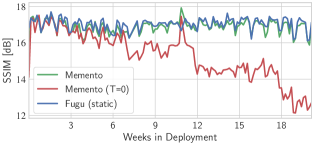
Figure 13. Long-term degradation of Memento ($T=0$) over time in a previous deployment on Puffer.)

Prediction score improvements compared to the past

Fig. 14 shows Fig. 6(a) overlayed with the prediction score improvements of Fugu compared to Fugu_Feb in the past. These curves are not directly comparable, as they come from different periods of time and the underlying data may have shifted. However, we can see that daily retraining with random samples did not consistently improve the TTP tail score; it even worsened the tail score for $20\text{\,}\mathrm{\char 37\relax}$ of days. This may explain why daily retraining yields significantly smaller tail QoE improvements than retraining with samples selected by Memento, which consistently improves the tail predictions.

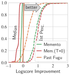
Figure 14. Retraining with daily samples did not consistently improve the tail prediction score in the past.

Alternative selection metrics

Fig. 21 shows further alternative sample selection metrics in addition to loss (Section 4.4).

Fig. 21(a) shows the results for model confidence, i.e., the probability of the predicted transmission time bin (Puffer separates the transmit time into 21 bins ranging from $0.125\text{\,}\mathrm{s}$ to $10\text{\,}\mathrm{s}$). With this metric, Memento prefers to discard samples with high confidence to keep ‘difficult’ samples with low confidence. For high temperatures, performance improvements are small. For low temperatures, we observe strong variation between runs, with more performance degradation than improvement. In summary, this selection metric is unreliable and fails to consistently improve performance.

Fig. 21(b) shows the results for label counts, a simplified version of density that is often used for classification data. We use the transmission time bin of each sample as the label. With this metric, Memento prefers to discard samples with high label counts to keep ‘rare’ samples with low label counts. We observe this approach to drastically reduce performance. In the Puffer environment, the majority of samples are assigned to the lowest transmit time bins. Going by label counts alone removes too many of these samples and the model forgets common patterns, similar to the loss metric.

Finally, Fig. 21(c) shows the results for stalled sessions. With this metric, Memento prefers to discard samples if they belong to a session that did not stall to keep samples from sessions that did stall. We observe consistent improvements, but they are small. It does not provide a fine-grained enough selection to significantly improve tail performance.

Increased memory capacity

Fig. 22 shows the results for Memento compared to a random memory with the same capacity (both $1\text{\,}\mathrm{M}$) and to a random memory with a double capacity ($2\text{\,}\mathrm{M}$). The random memory is set up like Fugu, selecting samples randomly over the last two weeks. We can see that simply increasing the capacity fails to address dataset imbalance, and performance is virtually identical at double the training effort.

Timeseries (replay)

Fig. 23 shows the evolution of each benchmark experiment over the whole 6-month duration. Fig. 24 and Fig. 25 show the same time series for the experiments with alternative selection metrics, and for combining Memento with Matchmaker and JTT, respectively.

For temperature-related benchmarks, we observe that a high temperature (uniformly random selection) performs slightly worse at the tail than Fugu. This may be because Fugu keeps samples from the past $14$ days, while a uniformly random selection phases samples out more quickly.

Appendix C Simulation: Supplemental Results

Simulation setup

Fig. 15 illustrates the setup we used for the evaluation of Memento in simulation.

Figure 15. Simulation setup.

Model Architecture

We use the following parameters for the classification and regression models used in our simulation experiments. We use supervised training and select the number of layers, neurons, and training parameters via hyperparameter optimization (headScikitoptimizeScikitoptimizeV02018, ).

We have implemented both models using Keras (cholletKeras2015, ). For all layers, we use batch normalization (ioffeBatchNormalizationAccelerating2015, ) and ReLU activation (nairRectifiedLinearUnits2010, ). We train both networks with the Adam optimizer (kingmaAdamMethodStochastic2017, ) using the default decay parameters $\beta_{1}=0.9,\ \beta_{2}=0.999$. We train for up $200$ epochs with early stopping.

	Model
Parameter	Classification	Regression
Hidden Layers	3	4
Hidden Units	512	362
Learning Batchsize	512	512
Learning Rate	$5.91\text{\times}{10}^{-5}$	0.382

Table 1. Model parameters.

Figure 16. Message size distributions (montazeriHomaReceiverdrivenLowlatency2018, ).

Workload distributions

Fig. 16 shows the message size distribution for the workloads we use, published by the HOMA project  (montazeriHomaReceiverdrivenLowlatency2018, )): Facebook web server (W1), DC-TCP (W2), and Facebook Hadoop (W3). Messages are generated with Poisson-distributed inter-arrival times.

Samples in memory

Table 2 shows the number of samples in memory after the last iteration of Section 5.2 and Section 5.3. Memento retains all workloads in memory, whereas other approaches either forget existing or fail to pick up new samples.

	W1	W2	W3
Rare Patterns (Section 5.2)
Memento	5696	9053	5219
Random	252	19634	114
LARS	3159	14231	2610
FIFO	0	20000	0
Incremental Learning (Section 5.3)
Memento	5376	5888	8704
Random	1266	17836	898
LARS	9540	9557	903
FIFO	0	0	20000

Table 2. In-memory samples after each experiment.

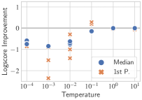
(a) Confidence

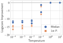
(b) Label counts

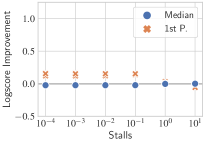
(c) Stalled sessions

Figure 21. Additional alternative selection metrics.

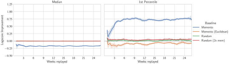
(a) Memento ($1\text{\,}\mathrm{M}$ samples) compared to random sampling like Fugu ($1\text{\,}\mathrm{M}$ and $2\text{\,}\mathrm{M}$ samples respectively) and compared to a Memento variant using the Euclidean distance between batch averages instead of JSD.

Figure 22. Logscore improvements compared to Fugu, concretely the median and tail (1st percentile) improvements for each day. We compute the mean over all three $6$-month replays, and plot again the mean of this value and bootstrapped 90% confidence intervals over two-week windows.

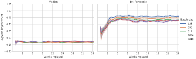
(a) Batch size.

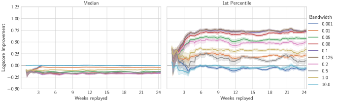
(b) Bandwidth

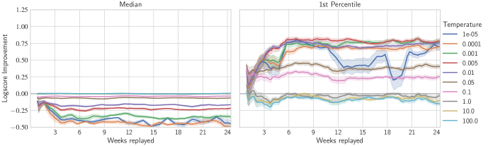
(c) Temperature

Figure 23. Logscore improvements compared to Fugu (see  Fig. 22) for all selection metric experiments.

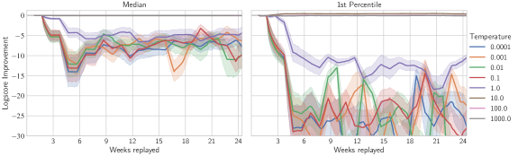
(a) Loss.

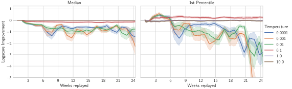
(b) Confidence.

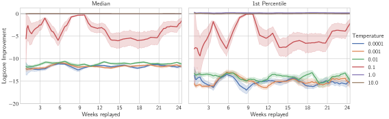
(c) Label counts

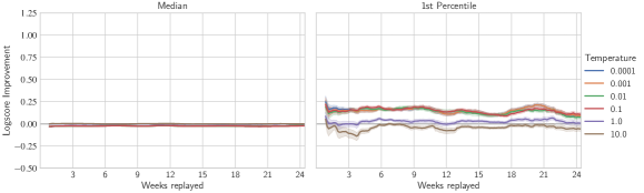
(d) Stalled sessions

Figure 24. Logscore improvements compared to Fugu (see  Fig. 22) for all selection metric experiments.

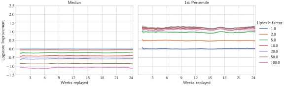
(a) JTT with random sample selection.

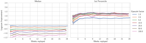
(b) JTT with Memento’s sample selection.

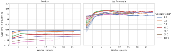
(c) JTT with Memento’s sample selection and optimal Matchmaker predictions.

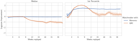
(d) Memento compared to Query-By-Committee (QBC) sample selection, both with optimal Matchmaker predictions.

Figure 25. Logscore improvements compared to Fugu (see  Fig. 22) for all combination experiments.

References

- (1) Puffer. URL: https://puffer.stanford.edu/.
- (2) YouTube Statistics 2024 [Users by Country + Demographics], February 2024. URL: https://www.globalmediainsight.com/blog/youtube-users-statistics/.
- (3) Soheil Abbasloo, Chen-Yu Yen, and H. Jonathan Chao. Classic Meets Modern: A Pragmatic Learning-Based Congestion Control for the Internet. In Proceedings of the Annual Conference of the ACM Special Interest Group on Data Communication on the Applications, Technologies, Architectures, and Protocols for Computer Communication, pages 632–647, Virtual Event USA, July 2020. ACM. URL: https://dl.acm.org/doi/10.1145/3387514.3405892, https://doi.org/10.1145/3387514.3405892.
- (4) Rahaf Aljundi, Eugene Belilovsky, Tinne Tuytelaars, Laurent Charlin, Massimo Caccia, Min Lin, and Lucas Page-Caccia. Online Continual Learning with Maximal Interfered Retrieval. In H. Wallach, H. Larochelle, A. Beygelzimer, F. d’ Alché-Buc, E. Fox, and R. Garnett, editors, Advances in Neural Information Processing Systems 32, pages 11849–11860. Curran Associates, Inc., 2019. URL: http://papers.nips.cc/paper/9357-online-continual-learning-with-maximal-interfered-retrieval.pdf.
- (5) Behnaz Arzani, Kevin Hsieh, and Haoxian Chen. Interpretable Feedback for AutoML and a Proposal for Domain-customized AutoML for Networking. In Proceedings of the Twentieth ACM Workshop on Hot Topics in Networks, HotNets ’21, pages 53–60, New York, NY, USA, November 2021. Association for Computing Machinery. https://doi.org/10.1145/3484266.3487373.
- (6) Eytan Bakshy. Real-world Video Adaptation with Reinforcement Learning. April 2019. URL: https://openreview.net/forum?id=SJlCkwN8iV.
- (7) Mihovil Bartulovic, Junchen Jiang, Sivaraman Balakrishnan, Vyas Sekar, and Bruno Sinopoli. Biases in Data-Driven Networking, and What to Do About Them. In Proceedings of the 16th ACM Workshop on Hot Topics in Networks, HotNets-XVI, pages 192–198, New York, NY, USA, November 2017. Association for Computing Machinery. https://doi.org/10.1145/3152434.3152448.
- (8) Abeba Birhane, Vinay Prabhu, Sang Han, Vishnu Naresh Boddeti, and Alexandra Sasha Luccioni. Into the LAIONs Den: Investigating Hate in Multimodal Datasets, November 2023. URL: http://arxiv.org/abs/2311.03449, arXiv:2311.03449, https://doi.org/10.48550/arXiv.2311.03449.
- (9) Coralie Busse-Grawitz, Roland Meier, Alexander Dietmüller, Tobias Bühler, and Laurent Vanbever. pForest: In-Network Inference with Random Forests, September 2019. URL: http://arxiv.org/abs/1909.05680, arXiv:1909.05680, https://doi.org/10.48550/arXiv.1909.05680.
- (10) Pietro Buzzega, Matteo Boschini, Angelo Porrello, and Simone Calderara. Rethinking Experience Replay: A Bag of Tricks for Continual Learning. arXiv:2010.05595 [cs, stat], October 2020. URL: http://arxiv.org/abs/2010.05595, arXiv:2010.05595.
- (11) Li Chen, Justinas Lingys, Kai Chen, and Feng Liu. AuTO: Scaling deep reinforcement learning for datacenter-scale automatic traffic optimization. In Proceedings of the 2018 Conference of the ACM Special Interest Group on Data Communication, SIGCOMM ’18, pages 191–205, New York, NY, USA, August 2018. Association for Computing Machinery. https://doi.org/10.1145/3230543.3230551.
- (12) François Chollet et al. Keras. 2015. URL: https://keras.io.
- (13) T. de Bruin, J. Kober, K. Tuyls, and R. Babuška. Improved deep reinforcement learning for robotics through distribution-based experience retention. In 2016 IEEE/RSJ International Conference on Intelligent Robots and Systems (IROS), pages 3947–3952, October 2016. https://doi.org/10.1109/IROS.2016.7759581.
- (14) Jacob Devlin, Ming-Wei Chang, Kenton Lee, and Kristina Toutanova. BERT: Pre-training of Deep Bidirectional Transformers for Language Understanding. arXiv:1810.04805 [cs], May 2019. URL: http://arxiv.org/abs/1810.04805, arXiv:1810.04805.
- (15) Alexander Dietmüller, Siddhant Ray, Romain Jacob, and Laurent Vanbever. A new hope for network model generalization. In HotNets ’22: Proceedings of the 21st ACM Workshop on Hot Topics in Networks, pages 152–159, New York, NY, November 2022. Association for Computing Machinery / ETHZ and ETHZ. https://doi.org/10.3929/ethz-b-000577569.
- (16) Gregory Ditzler, Manuel Roveri, Cesare Alippi, and Robi Polikar. Learning in Nonstationary Environments: A Survey. IEEE Computational Intelligence Magazine, 10(4):12–25, November 2015. https://doi.org/10.1109/MCI.2015.2471196.
- (17) Zhengfang Duanmu, Kai Zeng, Kede Ma, Abdul Rehman, and Zhou Wang. A Quality-of-Experience Index for Streaming Video. IEEE Journal of Selected Topics in Signal Processing, 11(1):154–166, February 2017. https://doi.org/10.1109/JSTSP.2016.2608329.
- (18) Vojislav Dukić, Sangeetha Abdu Jyothi, Bojan Karlas, Muhsen Owaida, Ce Zhang, and Ankit Singla. Is advance knowledge of flow sizes a plausible assumption? In 16th USENIX Symposium on Networked Systems Design and Implementation (NSDI 19), pages 565–580, Boston, MA, February 2019. USENIX Association. URL: https://www.usenix.org/conference/nsdi19/presentation/dukic.
- (19) Tomer Eliyahu, Yafim Kazak, Guy Katz, and Michael Schapira. Verifying learning-augmented systems. In Proceedings of the 2021 ACM SIGCOMM 2021 Conference, SIGCOMM ’21, pages 305–318, New York, NY, USA, August 2021. Association for Computing Machinery. https://doi.org/10.1145/3452296.3472936.
- (20) D. M. Endres and J. E. Schindelin. A new metric for probability distributions. IEEE Transactions on Information Theory, 49(7):1858–1860, July 2003.
- (21) Sebastian Farquhar and Yarin Gal. Towards Robust Evaluations of Continual Learning. arXiv:1805.09733 [cs, stat], June 2019. URL: http://arxiv.org/abs/1805.09733, arXiv:1805.09733.
- (22) Tilmann Gneiting and Adrian E. Raftery. Strictly Proper Scoring Rules, Prediction, and Estimation. Journal of the American Statistical Association, 102(477):359–378, March 2007. https://doi.org/10.1198/016214506000001437.
- (23) Chuan Guo, Geoff Pleiss, Yu Sun, and Kilian Q. Weinberger. On Calibration of Modern Neural Networks, August 2017. URL: http://arxiv.org/abs/1706.04599, arXiv:1706.04599, https://doi.org/10.48550/arXiv.1706.04599.
- (24) Kai Han, Yunhe Wang, Hanting Chen, Xinghao Chen, Jianyuan Guo, Zhenhua Liu, Yehui Tang, An Xiao, Chunjing Xu, Yixing Xu, Zhaohui Yang, Yiman Zhang, and Dacheng Tao. A Survey on Vision Transformer. IEEE Transactions on Pattern Analysis and Machine Intelligence, pages 1–1, 2022. https://doi.org/10.1109/TPAMI.2022.3152247.
- (25) Xin He, Kaiyong Zhao, and Xiaowen Chu. AutoML: A survey of the state-of-the-art. Knowledge-Based Systems, 212:106622, January 2021. URL: https://www.sciencedirect.com/science/article/pii/S0950705120307516, https://doi.org/10.1016/j.knosys.2020.106622.
- (26) Tim Head, MechCoder, Gilles Louppe, Iaroslav Shcherbatyi, fcharras, Zé Vinícius, cmmalone, Christopher Schröder, nel215, Nuno Campos, Todd Young, Stefano Cereda, Thomas Fan, rene-rex, Kejia (KJ) Shi, Justus Schwabedal, carlosdanielcsantos, Hvass-Labs, Mikhail Pak, SoManyUsernamesTaken, Fred Callaway, Loïc Estève, Lilian Besson, Mehdi Cherti, Karlson Pfannschmidt, Fabian Linzberger, Christophe Cauet, Anna Gut, Andreas Mueller, and Alexander Fabisch. Scikit-optimize/scikit-optimize: V0.5.2. Zenodo, March 2018. URL: https://zenodo.org/record/1207017, https://doi.org/10.5281/zenodo.1207017.
- (27) Fabian Hinder, André Artelt, and Barbara Hammer. Towards Non-Parametric Drift Detection via Dynamic Adapting Window Independence Drift Detection (DAWIDD). In Proceedings of the 37th International Conference on Machine Learning, pages 4249–4259. PMLR, November 2020. URL: https://proceedings.mlr.press/v119/hinder20a.html.
- (28) Sergey Ioffe and Christian Szegedy. Batch Normalization: Accelerating Deep Network Training by Reducing Internal Covariate Shift. In International Conference on Machine Learning, pages 448–456. PMLR, June 2015. URL: http://proceedings.mlr.press/v37/ioffe15.html.
- (29) David Isele and Akansel Cosgun. Selective Experience Replay for Lifelong Learning. arXiv:1802.10269 [cs], February 2018. URL: http://arxiv.org/abs/1802.10269, arXiv:1802.10269.
- (30) Nathan Jay, Noga Rotman, Brighten Godfrey, Michael Schapira, and Aviv Tamar. A Deep Reinforcement Learning Perspective on Internet Congestion Control. In Proceedings of the 36th International Conference on Machine Learning, pages 3050–3059. PMLR, May 2019. URL: https://proceedings.mlr.press/v97/jay19a.html.
- (31) Suraj Jog, Zikun Liu, Antonio Franques, Vimuth Fernando, Sergi Abadal, Josep Torrellas, and Haitham Hassanieh. One Protocol to Rule Them All: Wireless {Network-on-Chip} using Deep Reinforcement Learning. In 18th USENIX Symposium on Networked Systems Design and Implementation (NSDI 21), pages 973–989, 2021. URL: https://www.usenix.org/conference/nsdi21/presentation/jog.
- (32) Salman Khan, Muzammal Naseer, Munawar Hayat, Syed Waqas Zamir, Fahad Shahbaz Khan, and Mubarak Shah. Transformers in Vision: A Survey. ACM Computing Surveys, December 2021. https://doi.org/10.1145/3505244.
- (33) Diederik P. Kingma and Jimmy Ba. Adam: A Method for Stochastic Optimization. arXiv:1412.6980 [cs], January 2017. URL: http://arxiv.org/abs/1412.6980, arXiv:1412.6980.
- (34) James Kirkpatrick, Razvan Pascanu, Neil Rabinowitz, Joel Veness, Guillaume Desjardins, Andrei A. Rusu, Kieran Milan, John Quan, Tiago Ramalho, Agnieszka Grabska-Barwinska, Demis Hassabis, Claudia Clopath, Dharshan Kumaran, and Raia Hadsell. Overcoming catastrophic forgetting in neural networks. Proceedings of the National Academy of Sciences, 114(13):3521–3526, March 2017. URL: https://www.pnas.org/content/114/13/3521, https://doi.org/10.1073/pnas.1611835114.
- (35) S. Shunmuga Krishnan and Ramesh K. Sitaraman. Video Stream Quality Impacts Viewer Behavior: Inferring Causality Using Quasi-Experimental Designs. IEEE/ACM Transactions on Networking, 21(6):2001–2014, December 2013. https://doi.org/10.1109/TNET.2013.2281542.
- (36) S. Kullback and R. A. Leibler. On Information and Sufficiency. The Annals of Mathematical Statistics, 22(1):79–86, 1951. URL: https://www.jstor.org/stable/2236703, arXiv:2236703.
- (37) Adam Langley, Alistair Riddoch, Alyssa Wilk, Antonio Vicente, Charles Krasic, Dan Zhang, Fan Yang, Fedor Kouranov, Ian Swett, Janardhan Iyengar, Jeff Bailey, Jeremy Dorfman, Jim Roskind, Joanna Kulik, Patrik Westin, Raman Tenneti, Robbie Shade, Ryan Hamilton, Victor Vasiliev, Wan-Teh Chang, and Zhongyi Shi. The QUIC Transport Protocol: Design and Internet-Scale Deployment. In Proceedings of the Conference of the ACM Special Interest Group on Data Communication, SIGCOMM ’17, pages 183–196, New York, NY, USA, August 2017. Association for Computing Machinery. https://doi.org/10.1145/3098822.3098842.
- (38) Franck Le, Mudhakar Srivatsa, Raghu Ganti, and Vyas Sekar. Rethinking data-driven networking with foundation models: Challenges and opportunities. In Proceedings of the 21st ACM Workshop on Hot Topics in Networks, HotNets ’22, pages 188–197, New York, NY, USA, November 2022. Association for Computing Machinery. URL: https://dl.acm.org/doi/10.1145/3563766.3564109, https://doi.org/10.1145/3563766.3564109.
- (39) Zachary C. Lipton, Yu-Xiang Wang, and Alex Smola. Detecting and Correcting for Label Shift with Black Box Predictors. arXiv:1802.03916 [cs, stat], July 2018. URL: http://arxiv.org/abs/1802.03916, arXiv:1802.03916.
- (40) Evan Z. Liu, Behzad Haghgoo, Annie S. Chen, Aditi Raghunathan, Pang Wei Koh, Shiori Sagawa, Percy Liang, and Chelsea Finn. Just Train Twice: Improving Group Robustness without Training Group Information. In Proceedings of the 38th International Conference on Machine Learning, pages 6781–6792. PMLR, July 2021. URL: https://proceedings.mlr.press/v139/liu21f.html.
- (41) Shayne Longpre, Gregory Yauney, Emily Reif, Katherine Lee, Adam Roberts, Barret Zoph, Denny Zhou, Jason Wei, Kevin Robinson, David Mimno, and Daphne Ippolito. A Pretrainer’s Guide to Training Data: Measuring the Effects of Data Age, Domain Coverage, Quality, & Toxicity, November 2023. URL: http://arxiv.org/abs/2305.13169, arXiv:2305.13169, https://doi.org/10.48550/arXiv.2305.13169.
- (42) Ankur Mallick, Kevin Hsieh, Behnaz Arzani, and Gauri Joshi. Matchmaker: Data Drift Mitigation in Machine Learning for Large-Scale Systems. Proceedings of Machine Learning and Systems, 4:77–94, April 2022. URL: https://proceedings.mlsys.org/paper/2022/hash/1c383cd30b7c298ab50293adfecb7b18-Abstract.html.
- (43) Hongzi Mao, Ravi Netravali, and Mohammad Alizadeh. Neural Adaptive Video Streaming with Pensieve. In Proceedings of the Conference of the ACM Special Interest Group on Data Communication, SIGCOMM ’17, pages 197–210, Los Angeles, CA, USA, August 2017. Association for Computing Machinery. https://doi.org/10.1145/3098822.3098843.
- (44) James L. McClelland, Bruce L. McNaughton, and Randall C. O’Reilly. Why there are complementary learning systems in the hippocampus and neocortex: Insights from the successes and failures of connectionist models of learning and memory. Psychological Review, 102(3):419–457, 1995. https://doi.org/10.1037/0033-295X.102.3.419.
- (45) Rajdeep Mondal, Alan Tang, Ryan Beckett, Todd Millstein, and George Varghese. What do LLMs need to Synthesize Correct Router Configurations? In Proceedings of the 22nd ACM Workshop on Hot Topics in Networks, HotNets ’23, pages 189–195, New York, NY, USA, November 2023. Association for Computing Machinery. URL: https://dl.acm.org/doi/10.1145/3626111.3628194, https://doi.org/10.1145/3626111.3628194.
- (46) Behnam Montazeri, Yilong Li, Mohammad Alizadeh, and John Ousterhout. Homa: A receiver-driven low-latency transport protocol using network priorities. In Proceedings of the 2018 Conference of the ACM Special Interest Group on Data Communication, SIGCOMM ’18, pages 221–235, Budapest, Hungary, August 2018. Association for Computing Machinery. https://doi.org/10.1145/3230543.3230564.
- (47) Sudipto Mukherjee, Himanshu Asnani, Eugene Lin, and Sreeram Kannan. ClusterGAN: Latent Space Clustering in Generative Adversarial Networks. Proceedings of the AAAI Conference on Artificial Intelligence, 33(01):4610–4617, July 2019. URL: https://ojs.aaai.org/index.php/AAAI/article/view/4385, https://doi.org/10.1609/aaai.v33i01.33014610.
- (48) Vinod Nair and Geoffrey E. Hinton. Rectified linear units improve restricted Boltzmann machines. In Johannes Fürnkranz and Thorsten Joachims, editors, Proceedings of the 27th International Conference on Machine Learning (ICML-10), pages 807–814, Haifa, Israel, June 2010. Omnipress. URL: http://www.icml2010.org/papers/432.pdf.
- (49) X. Nie, Y. Zhao, Z. Li, G. Chen, K. Sui, J. Zhang, Z. Ye, and D. Pei. Dynamic TCP Initial Windows and Congestion Control Schemes Through Reinforcement Learning. IEEE Journal on Selected Areas in Communications, 37(6):1231–1247, June 2019. https://doi.org/10.1109/JSAC.2019.2904350.
- (50) OpenAI, Josh Achiam, Steven Adler, Sandhini Agarwal, Lama Ahmad, Ilge Akkaya, Florencia Leoni Aleman, Diogo Almeida, Janko Altenschmidt, Sam Altman, Shyamal Anadkat, Red Avila, Igor Babuschkin, Suchir Balaji, Valerie Balcom, Paul Baltescu, Haiming Bao, Mo Bavarian, Jeff Belgum, Irwan Bello, Jake Berdine, Gabriel Bernadett-Shapiro, Christopher Berner, Lenny Bogdonoff, Oleg Boiko, Madelaine Boyd, Anna-Luisa Brakman, Greg Brockman, Tim Brooks, Miles Brundage, Kevin Button, Trevor Cai, Rosie Campbell, Andrew Cann, Brittany Carey, Chelsea Carlson, Rory Carmichael, Brooke Chan, Che Chang, Fotis Chantzis, Derek Chen, Sully Chen, Ruby Chen, Jason Chen, Mark Chen, Ben Chess, Chester Cho, Casey Chu, Hyung Won Chung, Dave Cummings, Jeremiah Currier, Yunxing Dai, Cory Decareaux, Thomas Degry, Noah Deutsch, Damien Deville, Arka Dhar, David Dohan, Steve Dowling, Sheila Dunning, Adrien Ecoffet, Atty Eleti, Tyna Eloundou, David Farhi, Liam Fedus, Niko Felix, Simón Posada Fishman, Juston Forte, Isabella Fulford, Leo Gao, Elie Georges, Christian Gibson, Vik Goel, Tarun Gogineni, Gabriel Goh, Rapha Gontijo-Lopes, Jonathan Gordon, Morgan Grafstein, Scott Gray, Ryan Greene, Joshua Gross, Shixiang Shane Gu, Yufei Guo, Chris Hallacy, Jesse Han, Jeff Harris, Yuchen He, Mike Heaton, Johannes Heidecke, Chris Hesse, Alan Hickey, Wade Hickey, Peter Hoeschele, Brandon Houghton, Kenny Hsu, Shengli Hu, Xin Hu, Joost Huizinga, Shantanu Jain, Shawn Jain, Joanne Jang, Angela Jiang, Roger Jiang, Haozhun Jin, Denny Jin, Shino Jomoto, Billie Jonn, Heewoo Jun, Tomer Kaftan, Łukasz Kaiser, Ali Kamali, Ingmar Kanitscheider, Nitish Shirish Keskar, Tabarak Khan, Logan Kilpatrick, Jong Wook Kim, Christina Kim, Yongjik Kim, Hendrik Kirchner, Jamie Kiros, Matt Knight, Daniel Kokotajlo, Łukasz Kondraciuk, Andrew Kondrich, Aris Konstantinidis, Kyle Kosic, Gretchen Krueger, Vishal Kuo, Michael Lampe, Ikai Lan, Teddy Lee, Jan Leike, Jade Leung, Daniel Levy, Chak Ming Li, Rachel Lim, Molly Lin, Stephanie Lin, Mateusz Litwin, Theresa Lopez, Ryan Lowe, Patricia Lue, Anna Makanju, Kim Malfacini, Sam Manning, Todor Markov, Yaniv Markovski, Bianca Martin, Katie Mayer, Andrew Mayne, Bob McGrew, Scott Mayer McKinney, Christine McLeavey, Paul McMillan, Jake McNeil, David Medina, Aalok Mehta, Jacob Menick, Luke Metz, Andrey Mishchenko, Pamela Mishkin, Vinnie Monaco, Evan Morikawa, Daniel Mossing, Tong Mu, Mira Murati, Oleg Murk, David Mély, Ashvin Nair, Reiichiro Nakano, Rajeev Nayak, Arvind Neelakantan, Richard Ngo, Hyeonwoo Noh, Long Ouyang, Cullen O’Keefe, Jakub Pachocki, Alex Paino, Joe Palermo, Ashley Pantuliano, Giambattista Parascandolo, Joel Parish, Emy Parparita, Alex Passos, Mikhail Pavlov, Andrew Peng, Adam Perelman, Filipe de Avila Belbute Peres, Michael Petrov, Henrique Ponde de Oliveira Pinto, Michael, Pokorny, Michelle Pokrass, Vitchyr Pong, Tolly Powell, Alethea Power, Boris Power, Elizabeth Proehl, Raul Puri, Alec Radford, Jack Rae, Aditya Ramesh, Cameron Raymond, Francis Real, Kendra Rimbach, Carl Ross, Bob Rotsted, Henri Roussez, Nick Ryder, Mario Saltarelli, Ted Sanders, Shibani Santurkar, Girish Sastry, Heather Schmidt, David Schnurr, John Schulman, Daniel Selsam, Kyla Sheppard, Toki Sherbakov, Jessica Shieh, Sarah Shoker, Pranav Shyam, Szymon Sidor, Eric Sigler, Maddie Simens, Jordan Sitkin, Katarina Slama, Ian Sohl, Benjamin Sokolowsky, Yang Song, Natalie Staudacher, Felipe Petroski Such, Natalie Summers, Ilya Sutskever, Jie Tang, Nikolas Tezak, Madeleine Thompson, Phil Tillet, Amin Tootoonchian, Elizabeth Tseng, Preston Tuggle, Nick Turley, Jerry Tworek, Juan Felipe Cerón Uribe, Andrea Vallone, Arun Vijayvergiya, Chelsea Voss, Carroll Wainwright, Justin Jay Wang, Alvin Wang, Ben Wang, Jonathan Ward, Jason Wei, C. J. Weinmann, Akila Welihinda, Peter Welinder, Jiayi Weng, Lilian Weng, Matt Wiethoff, Dave Willner, Clemens Winter, Samuel Wolrich, Hannah Wong, Lauren Workman, Sherwin Wu, Jeff Wu, Michael Wu, Kai Xiao, Tao Xu, Sarah Yoo, Kevin Yu, Qiming Yuan, Wojciech Zaremba, Rowan Zellers, Chong Zhang, Marvin Zhang, Shengjia Zhao, Tianhao Zheng, Juntang Zhuang, William Zhuk, and Barret Zoph. GPT-4 Technical Report, December 2023. URL: http://arxiv.org/abs/2303.08774, arXiv:2303.08774, https://doi.org/10.48550/arXiv.2303.08774.
- (51) German I. Parisi, Ronald Kemker, Jose L. Part, Christopher Kanan, and Stefan Wermter. Continual lifelong learning with neural networks: A review. Neural Networks, 113:54–71, May 2019. URL: http://www.sciencedirect.com/science/article/pii/S0893608019300231, https://doi.org/10.1016/j.neunet.2019.01.012.
- (52) Emanuel Parzen. On Estimation of a Probability Density Function and Mode. The Annals of Mathematical Statistics, 33(3):1065–1076, 1962. URL: https://www.jstor.org/stable/2237880, arXiv:2237880.
- (53) Neoklis Polyzotis, Martin Zinkevich, Sudip Roy, Eric Breck, and Steven Whang. Data Validation for Machine Learning. In A. Talwalkar, V. Smith, and M. Zaharia, editors, Proceedings of Machine Learning and Systems, volume 1, pages 334–347, 2019. URL: https://proceedings.mlsys.org/paper/2019/file/5878a7ab84fb43402106c575658472fa-Paper.pdf.
- (54) P. Poupart, Z. Chen, P. Jaini, F. Fung, H. Susanto, Yanhui Geng, Li Chen, K. Chen, and Hao Jin. Online flow size prediction for improved network routing. In 2016 IEEE 24th International Conference on Network Protocols (ICNP), pages 1–6, November 2016. https://doi.org/10.1109/ICNP.2016.7785324.
- (55) Stephan Rabanser, Stephan Günnemann, and Zachary Lipton. Failing Loudly: An Empirical Study of Methods for Detecting Dataset Shift. In H. Wallach, H. Larochelle, A. Beygelzimer, F. d\textquotesingle Alché-Buc, E. Fox, and R. Garnett, editors, Advances in Neural Information Processing Systems 32, pages 1396–1408. Curran Associates, Inc., 2019. URL: http://papers.nips.cc/paper/8420-failing-loudly-an-empirical-study-of-methods-for-detecting-dataset-shift.pdf.
- (56) Roger Ratcliff. Connectionist models of recognition memory: Constraints imposed by learning and forgetting functions. Psychological Review, 97(2):285–308, 1990. https://doi.org/10.1037/0033-295X.97.2.285.
- (57) Martin Riedmiller. Neural fitted Q Iteration–First experiences with a data efficient neural reinforcement learning method. In European Conference on Machine Learning, pages 317–328, 2005.
- (58) George F. Riley and Thomas R. Henderson. The ns-3 Network Simulator. In Klaus Wehrle, Mesut Güneş, and James Gross, editors, Modeling and Tools for Network Simulation, pages 15–34. Springer, Berlin, Heidelberg, 2010. https://doi.org/10.1007/978-3-642-12331-3_2.
- (59) David Rolnick, Arun Ahuja, Jonathan Schwarz, Timothy Lillicrap, and Gregory Wayne. Experience Replay for Continual Learning. In H. Wallach, H. Larochelle, A. Beygelzimer, F. d’ Alché-Buc, E. Fox, and R. Garnett, editors, Advances in Neural Information Processing Systems 32, pages 350–360. Curran Associates, Inc., 2019. URL: http://papers.nips.cc/paper/8327-experience-replay-for-continual-learning.pdf.
- (60) Noga H. Rotman, Michael Schapira, and Aviv Tamar. Online Safety Assurance for Learning-Augmented Systems. In Proceedings of the 19th ACM Workshop on Hot Topics in Networks, HotNets ’20, pages 88–95, New York, NY, USA, November 2020. Association for Computing Machinery. https://doi.org/10.1145/3422604.3425940.
- (61) H. S. Seung, M. Opper, and H. Sompolinsky. Query by committee. In Proceedings of the Fifth Annual Workshop on Computational Learning Theory, COLT ’92, pages 287–294, New York, NY, USA, July 1992. Association for Computing Machinery. URL: https://dl.acm.org/doi/10.1145/130385.130417, https://doi.org/10.1145/130385.130417.
- (62) Hidetoshi Shimodaira. Improving predictive inference under covariate shift by weighting the log-likelihood function. Journal of Statistical Planning and Inference, 90(2):227–244, October 2000. URL: https://www.sciencedirect.com/science/article/pii/S0378375800001154, https://doi.org/10.1016/S0378-3758(00)00115-4.
- (63) Ashraf Tahmasbi, Ellango Jothimurugesan, Srikanta Tirthapura, and Phillip B. Gibbons. DriftSurf: Stable-State / Reactive-State Learning under Concept Drift. In Proceedings of the 38th International Conference on Machine Learning, pages 10054–10064. PMLR, July 2021. URL: https://proceedings.mlr.press/v139/tahmasbi21a.html.
- (64) Hugo Touvron, Louis Martin, Kevin Stone, Peter Albert, Amjad Almahairi, Yasmine Babaei, Nikolay Bashlykov, Soumya Batra, Prajjwal Bhargava, Shruti Bhosale, Dan Bikel, Lukas Blecher, Cristian Canton Ferrer, Moya Chen, Guillem Cucurull, David Esiobu, Jude Fernandes, Jeremy Fu, Wenyin Fu, Brian Fuller, Cynthia Gao, Vedanuj Goswami, Naman Goyal, Anthony Hartshorn, Saghar Hosseini, Rui Hou, Hakan Inan, Marcin Kardas, Viktor Kerkez, Madian Khabsa, Isabel Kloumann, Artem Korenev, Punit Singh Koura, Marie-Anne Lachaux, Thibaut Lavril, Jenya Lee, Diana Liskovich, Yinghai Lu, Yuning Mao, Xavier Martinet, Todor Mihaylov, Pushkar Mishra, Igor Molybog, Yixin Nie, Andrew Poulton, Jeremy Reizenstein, Rashi Rungta, Kalyan Saladi, Alan Schelten, Ruan Silva, Eric Michael Smith, Ranjan Subramanian, Xiaoqing Ellen Tan, Binh Tang, Ross Taylor, Adina Williams, Jian Xiang Kuan, Puxin Xu, Zheng Yan, Iliyan Zarov, Yuchen Zhang, Angela Fan, Melanie Kambadur, Sharan Narang, Aurelien Rodriguez, Robert Stojnic, Sergey Edunov, and Thomas Scialom. Llama 2: Open Foundation and Fine-Tuned Chat Models, July 2023. URL: http://arxiv.org/abs/2307.09288, arXiv:2307.09288, https://doi.org/10.48550/arXiv.2307.09288.
- (65) Asaf Valadarsky, Michael Schapira, Dafna Shahaf, and Aviv Tamar. Learning to Route. In Proceedings of the 16th ACM Workshop on Hot Topics in Networks, HotNets-XVI, pages 185–191, New York, NY, USA, 2017. ACM. URL: http://doi.acm.org/10.1145/3152434.3152441, https://doi.org/10.1145/3152434.3152441.
- (66) Hado van Hasselt, Arthur Guez, and David Silver. Deep Reinforcement Learning with Double Q-Learning. Proceedings of the AAAI Conference on Artificial Intelligence, 30(1), March 2016. URL: https://ojs.aaai.org/index.php/AAAI/article/view/10295.
- (67) Ashish Vaswani, Noam Shazeer, Niki Parmar, Jakob Uszkoreit, Llion Jones, Aidan N Gomez, Łukasz Kaiser, and Illia Polosukhin. Attention is all you need. In I. Guyon, U. V. Luxburg, S. Bengio, H. Wallach, R. Fergus, S. Vishwanathan, and R. Garnett, editors, Advances in Neural Information Processing Systems, volume 30. Curran Associates, Inc., 2017. URL: https://proceedings.neurips.cc/paper/2017/file/3f5ee243547dee91fbd053c1c4a845aa-Paper.pdf.
- (68) Matthias Wichtlhuber, Eric Strehle, Daniel Kopp, Lars Prepens, Stefan Stegmueller, Alina Rubina, Christoph Dietzel, and Oliver Hohlfeld. IXP scrubber: Learning from blackholing traffic for ML-driven DDoS detection at scale. In Proceedings of the ACM SIGCOMM 2022 Conference, SIGCOMM ’22, pages 707–722, New York, NY, USA, August 2022. Association for Computing Machinery. https://doi.org/10.1145/3544216.3544268.
- (69) Gerhard Widmer and Miroslav Kubat. Learning in the Presence of Concept Drift and Hidden Contexts. Machine Learning, 23(1):69–101, April 1996. https://doi.org/10.1023/A:1018046501280.
- (70) Keith Winstein and Hari Balakrishnan. TCP Ex Machina: Computer-generated Congestion Control. In Proceedings of the ACM SIGCOMM 2013 Conference on SIGCOMM, SIGCOMM ’13, pages 123–134, New York, NY, USA, 2013. ACM. URL: http://doi.acm.org/10.1145/2486001.2486020, https://doi.org/10.1145/2486001.2486020.
- (71) Sebastien C. Wong, Adam Gatt, Victor Stamatescu, and Mark D. McDonnell. Understanding Data Augmentation for Classification: When to Warp? In 2016 International Conference on Digital Image Computing: Techniques and Applications (DICTA), pages 1–6, November 2016. https://doi.org/10.1109/DICTA.2016.7797091.
- (72) Zhengxu Xia, Yajie Zhou, Francis Y. Yan, and Junchen Jiang. Automatic Curriculum Generation for Learning Adaptation in Networking, September 2022. URL: http://arxiv.org/abs/2202.05940, arXiv:2202.05940, https://doi.org/10.48550/arXiv.2202.05940.
- (73) Zhengxu Xia, Yajie Zhou, Francis Y. Yan, and Junchen Jiang. Genet: Automatic curriculum generation for learning adaptation in networking. In Proceedings of the ACM SIGCOMM 2022 Conference, SIGCOMM ’22, pages 397–413, New York, NY, USA, August 2022. Association for Computing Machinery. https://doi.org/10.1145/3544216.3544243.
- (74) Francis Y. Yan, Hudson Ayers, Chenzhi Zhu, Sadjad Fouladi, James Hong, Keyi Zhang, Philip Levis, and Keith Winstein. Learning in situ: A randomized experiment in video streaming. In 17th USENIX Symposium on Networked Systems Design and Implementation (NSDI 20), pages 495–511, 2020. URL: https://www.usenix.org/conference/nsdi20/presentation/yan.
- (75) Francis Y. Yan, Jestin Ma, Greg D. Hill, Deepti Raghavan, Riad S. Wahby, Philip Levis, and Keith Winstein. Pantheon: The training ground for Internet congestion-control research. In 2018 USENIX Annual Technical Conference (USENIX ATC 18), pages 731–743, 2018. URL: https://www.usenix.org/conference/atc18/presentation/yan-francis.
- (76) Yiding Yu, Taotao Wang, and Soung Chang Liew. Deep-Reinforcement Learning Multiple Access for Heterogeneous Wireless Networks. IEEE Journal on Selected Areas in Communications, 37(6):1277–1290, June 2019. https://doi.org/10.1109/JSAC.2019.2904329.
- (77) Friedemann Zenke, Ben Poole, and Surya Ganguli. Continual Learning Through Synaptic Intelligence. In International Conference on Machine Learning, pages 3987–3995. PMLR, July 2017. URL: http://proceedings.mlr.press/v70/zenke17a.html.
- (78) Qizhen Zhang, Kelvin K. W. Ng, Charles Kazer, Shen Yan, João Sedoc, and Vincent Liu. MimicNet: Fast performance estimates for data center networks with machine learning. In Proceedings of the 2021 ACM SIGCOMM 2021 Conference, SIGCOMM ’21, pages 287–304, New York, NY, USA, August 2021. Association for Computing Machinery. https://doi.org/10.1145/3452296.3472926.
- (79) Dora Zhao, Angelina Wang, and Olga Russakovsky. Understanding and Evaluating Racial Biases in Image Captioning. In Proceedings of the IEEE/CVF International Conference on Computer Vision, pages 14830–14840, 2021.
- (80) Zhou Wang, A. C. Bovik, H. R. Sheikh, and E. P. Simoncelli. Image quality assessment: From error visibility to structural similarity. IEEE Transactions on Image Processing, 13(4):600–612, April 2004. https://doi.org/10.1109/TIP.2003.819861.