Locating the critical point for the hadron to quark-gluon plasma phase transition from finite-size scaling of proton cumulants in heavy-ion collisions
Abstract
We perform a finite-size scaling analysis of net-proton number cumulants in Au+Au collisions at center-of-mass energies between GeV and 54.4 GeV to search for evidence of a critical point in the QCD phase diagram. In our analysis, we use both susceptibility and Binder cumulants which we extract from the second and fourth moments of the net-proton number distributions. We take measurements in different rapidity bin widths, corresponding to different subvolumes of the system, as probes of different length scales. We use model simulations to verify the applicability of this approach, then apply it to data and find evidence for a critical point near the baryon chemical potential of and temperature of MeV. The Binder cumulants, also analyzed in varying rapidity bin widths, provide complementary evidence for a critical point in a similar region. This is the first analysis of experimental data to locate the critical point in a range consistent with theoretical predictions.
I Introduction
Up until a few microseconds after the Big Bang, the strongly interacting matter in the Universe existed as a plasma of quarks and gluons. As the Universe expanded and cooled, this quark-gluon plasma underwent a phase change in which the quarks and gluons became confined into baryons and light nuclei Polyakov (1978); Susskind (1979). The early Universe had nearly identical numbers of baryons and antibaryons, so that its baryon chemical potential was very close to zero. After annihilation processes, the remaining small excess of baryons became the visible matter of our Universe, where baryonic matter exists in nuclei, the interiors of neutron stars, or, fleetingly, in systems created after nuclei collide either in cosmic ray interactions or at accelerator-based experiments. Properties of this matter both in its ground state as well as at extreme temperatures and densities shed light on the fundamental interactions and processes shaping our Universe. In heavy-ion experiments, the temperature and baryon density (or, equivalently, ) can be varied by changing the center-of-mass collision energy , thus probing large regions in the phase diagram of quantum chromodynamics (QCD) Collins and Perry (1975); Asakawa and Yazaki (1989); Braun-Munzinger and Stachel (1996); Fukushima and Sasaki (2013); Sorensen et al. (2024).
Despite its relevance to studies of neutron stars, the early evolution of the Universe, and nuclear matter properties, the phase diagram of strongly-interacting matter remains poorly known. This is particularly true at high values of , where first-principles lattice QCD calculations are stymied by the fermion sign problem which precludes direct calculations away from Karsch (2002). For example, although lattice calculations show that the hadron to quark-gluon plasma phase transition at is a smooth crossover Aoki et al. (2006); Ratti (2018), it is not yet known whether a critical point exists at higher where the smooth crossover transition would change to a first-order phase transition Asakawa and Yazaki (1989); Barducci et al. (1989); Halasz et al. (1998). The search for this potential critical point has been a high priority for the nuclear physics community for several decades Baym (2002). Lattice QCD calculations can still provide insight by circumventing the sign problem in at least two ways: 1) quantities calculated at can be used to extrapolate to Allton et al. (2002); Barbour et al. (1998), or 2) calculations in the imaginary -plane can be used in conjunction with the location of Lee-Yang edge singularities for the 3-D Ising model and the fact that QCD is known to be within the 3-D Ising universality class Pisarski and Wilczek (1984) to estimate the position of the critical point for QCD Johnson et al. (2023); Rennecke and Skokov (2022). The first method appears to exclude the presence of a critical point in the region characterized by Bollweg et al. (2022, 2023); Borsanyi et al. (2020, 2022), while the second method recently led to a preliminary prediction for a critical point near MeV and MeV Mukherjee and Skokov (2021); Connelly et al. (2021); Basar (2021); Dimopoulos et al. (2022); Zambello et al. (2023); Schmidt et al. (2023). The latter result places the critical point in a region recently probed by the STAR Collaboration measurements of heavy-ion collisions at the Relativistic Heavy Ion Collider (RHIC), exploring the QCD phase diagram through the Beam Energy Scan (BES) program and its fixed-target campaign Aggarwal et al. (2010); Odyniec (2019); Meehan (2016). In this work, we report on a novel finite-size scaling (FSS) analysis of data from the STAR experiment Abdallah et al. (2021, 2023) and the HADES experiment Adamczewski-Musch et al. (2020) at GSI, Germany, which probes even higher values of .
FSS is an approach originating from generic arguments considering relevant length scales and scale-free quantities Ferdinand and Fisher (1969); Cavagna et al. (2018). This analysis framework can be used to understand the behavior of systems with finite spatial dimensions, particularly near a critical point where the correlation length becomes large, and provides a systematic way to extrapolate the properties of a finite-sized system to the thermodynamic limit (where the system size approaches infinity). The key insight behind FSS lies in the observation that when the correlation length becomes of the order of the size of the system, physical observables exhibit a power-law scaling behavior that depends only on a few exponents (referred to as “critical exponents”) and universal scaling functions. By properly rescaling the system variables and observables, FSS allows one to not only accurately predict the behavior of thermodynamic quantities (such as correlation lengths, susceptibilities, or Binder cumulants Binder (1981)) as the system size changes, but also to identify the location of the critical point in the continuum limit. We present a brief pedagogical discussion of FSS in Appendix A.
In the context of heavy-ion collisions, FSS has been previously applied to search for the QCD critical point Palhares et al. (2011); Fraga et al. (2011); Lacey et al. (2016); in those studies, the system size was varied by selecting events from different collision centrality intervals, that is events originating at different initial overlaps of the colliding nuclei and thus involving different numbers of participating nucleons. There are two common disadvantages to these past applications of FSS: 1) the scaled variables used were not clearly related to correlation lengths, the susceptibility, or the order parameter of the system, and 2) the use of centrality classes to vary the system size introduced other confounding changes to the system such as differences in the temperature, system shape, and dynamical evolution which can potentially spoil the analysis.
The novel insight we utilize is that FSS can also be applied by calculating observables in subvolumes of varying size within systems of the same size Martin et al. (2021). This approach is particularly useful in a situation where one has limited ability to manipulate the parameters of the system, which is the case not only in heavy-ion collisions, but also in, e.g., biological systems. In addition, since FSS provides a method to make connections between different subvolume sizes, it allows one to jointly analyze data collected in experiments with different detector acceptance windows, alleviating many challenges to comparing experiments at different energies where, especially for fixed-target collisions, the detector acceptance changes with collision energy.
Illuminating arguments for applying FSS to subvolumes are laid out in Ref. Cavagna et al. (2018) which discusses bird flocks. Those arguments are then used in Ref. Martin et al. (2021) to extract the critical exponents for a neuronal network. Though more sophisticated renormalization group methods also verify the applicability of FSS, the generality of the arguments laid out in Refs. Cavagna et al. (2018); Martin et al. (2021) is remarkable and underlined by the vastly different contexts within which they are applicable: When the correlation length in a system grows large, then — as long as the size of the considered subvolume is large compared to any extraneous short-range correlations — the only relevant scale is defined by the size of the subvolume. In this case, extrapolating to an infinite subvolume yields a system with no scale, implying a power-law decay behavior of correlations and related quantities. From the power-law decay behavior, one can derive the usual expectations for FSS, such as the scaling law for the susceptibility :
| (1) |
where is the characteristic size of the system or subvolume, is the distance from the critical point such as , , or , is an unknown universal scaling function, and and are critical exponents which are the same for any system belonging to a given universality class, irrespective of the details of microscopic interactions. It is known that QCD is in the 3-D Ising universality class Pisarski and Wilczek (1984) where and Sengers and Shanks (2009). Based on Eq. (1), if is plotted as a function of , then data for different system sizes and values of should collapse on a single universal curve ; the crucial insight for using FSS in finding the critical point is that this can only take place when the correct value of , , or is used in . Thus, scanning ranges of values of or until the data collapse occurs provides a valuable method to determine the location of a critical point.
One may, nevertheless, question the applicability of FSS to heavy-ion experiments based on the short lifetime of the collisions Nonaka and Asakawa (2005); Nahrgang et al. (2019); Stephanov and Yin (2018), which may prevent the correlation length from growing large enough, and the presence of other short-range correlations which create dependencies outside of the FSS framework. In our analysis, we use rapidity windows to define the subvolume size. Then for FSS to apply, we need , where is separation in rapidity related to some interparticle correlation not associated with the diverging thermodynamic correlation length , the latter corresponding to an extent in rapidity . Given the small size of systems created in heavy-ion collisions and the typical size characterizing short-range correlations such as the Hanburry–Brown-Twiss (HBT) correlations or resonance decays, the regime of applicability may indeed appear narrow. However, it is important to note that the number of particle pairs affected by the aforementioned short-range correlations is proportional to the number of particles , while the collective correlations (driven, for example, by phase separation) will scale more closely with . Because of this, even if is not negligible, in many cases the spurious correlations are suppressed relative to the collective correlations of interest by . Regarding the lifetime of the system, we presume that in an analysis based on rapidity windows, the constraint on the correlations stemming from the window size up to at most one unit of rapidity is likely more restricting than the constraint arising from the final evolution time of the system; in other words, although the correlations may take a long time to reach their thermodynamic expectations, it will take them a much shorter time to exceed the lengths commensurate with our rapidity windows, thus satisfying the need for the system to be approximately scale-free. We also note that models assuming global or local thermalization, such as the hadron resonance gas model or hydrodynamic models, tend to work surprisingly well in descriptions of heavy-ion collisions despite concerns about both the timescale and the mechanisms by which the system thermalizes.
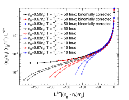
Some tests of the application of the FFS technique to finite subvolumes of dynamically evolving systems can be performed in microscopic transport simulations. Here, we simulate uniform nuclear matter, interacting through mean-field potentials corresponding to an equation of state with a critical point Sorensen and Koch (2021), in a box with periodic boundary conditions at a series of different densities. After the system equilibrates, we calculate the baryon susceptibility (see Sec. II) for a series of subvolumes. The importance of effects due to baryon number conservation is clearly seen by comparing the scaling behavior of results corrected Vovchenko et al. (2020); Kuznietsov et al. (2022) for conservation effects (solid circles) to uncorrected data (empty circles). Scaling the corrected data using the (known) value of the critical density and mean-field critical exponents yields a universal curve, with minuscule deviations only at the largest subvolumes, while the uncorrected data fails to scale for subvolume sizes larger than 25% of the total volume. For smaller subvolumes, however, the results exhibit the expected scaling; we note that the best scaling behavior in this case is obtained for , that is within 3% of the true value. Simulations also allow us to assess the influence of considering systems which only approach equilibrium. To this end, we consider points obtained relatively early in the evolution (empty triangles) when, in our simulations, the cumulants have only developed about 60% of their final time, equilibrated values. In this case, finite-size scaling is likewise not achieved for volume fractions larger than 25% of the total volume, and the best scaling behavior is attained for .
While acknowledging that there are legitimate questions about the details of the underlying systems which may challenge a FSS data analysis, we believe that the model results presented above provide ample justification to pursue this direction.
II Observables and data
The cumulants, central moments, and susceptibilities are related as follows,
| (2) | ||||
| (3) | ||||
| (4) | ||||
| (5) |
where denotes the th order cumulant, denotes the th central moment, is the th order susceptibility, and is the volume. We note that in the context of the QCD phase diagram, refers to susceptibilities of the baryon number, while the data at hand is limited to moments and cumulants of protons. This introduces a mismatch between the experimental observables and the susceptibility defined through derivatives with respect to . However, it has been argued Hatta and Stephanov (2003) that the singular parts of baryon susceptibility and proton number fluctuations coincide, which indicates that the corresponding power laws are the same in both cases even if the individual susceptibilities differ in a non-trivial way. Nevertheless, we have also checked the consequences of attempting to convert the net proton cumulants to net baryon cumulants under the assumptions used in Ref. Kitazawa and Asakawa (2012), and we discuss the consequences in Sec. III. In addition to finite-size scaling of the susceptibility, we will also consider the Binder cumulant, which is related to and as follows,
| (6) |
and provides another method to search for evidence of a critical point. Binder cumulants Binder (1981) were first proposed for studying the phase transition in the Ising model, where the distribution of the order parameter is Gaussian () at temperatures above the critical temperature, but becomes bimodal () in the phase coexistence region. Finite-size effects will prevent the system from reaching these continuum limit expectations. At the critical point, however, all finite system sizes are equivalently small compared to the infinite, continuum-limit correlation length and the Binder cumulant will become independent of the system size. The generic expectation is that Binder cumulants calculated as a function of different system sizes or system subvolumes should cross at the critical point. Binder cumulants have also been used in the context of lattice QCD to identify the critical point in the plane defined by temperature and quark masses Fukugita et al. (1990); Karsch et al. (2001).
Typically, cumulant measurements are presented as cumulant ratios, so that the term in Eqs. (2)–(5) drops out, leaving ratios of susceptibilities. However, in our analysis we are interested in the susceptibilities, and in particular in the second order susceptibility . To extract from data, we use the published chemical freeze-out parameters from thermal model fits to the measured particle yields to determine Andronic et al. (2018). The thermal model parameters include the temperature at the chemical freeze-out , the baryon chemical potential at the chemical freeze-out , and the volume per unit rapidity . The susceptibility in our analysis is then
| (7) |
where is the rapidity bin width, i.e., the rapidity window defining the subvolume, and is the volume associated with that rapidity bin.
We use data measured in 0–5%-central Au+Au collisions at , 3.0, 7.7, 11.5, 14.5, 19.6, 27, 39, and 54.4 GeV. The 7.7 – 54.4 GeV data are from collisions measured by STAR in the collider mode Abdallah et al. (2021) while the 2.4 and 3.0 GeV data sets were collected from fixed-target collisions at HADES Adamczewski-Musch et al. (2020) and STAR Abdallah et al. (2023), respectively. For the FSS analysis, one would like to only change the volume and the distance from the critical point while keeping all other aspects of the system fixed. As already argued above, using central collisions at each energy provides more uniform control over the data than comparing different collision centrality classes as was done in previous FSS analyses applied to heavy-ion collisions. Moreover, central collisions require smaller volume fluctuation corrections since an upper limit on the initial size of the system is set by the size of the nuclei being collided, thus reducing the systematic uncertainty on the corrections. We note, however, that for collisions at and 3.0 GeV the net-baryon density and the particle ratios change substantially as the rapidity window increases STA (2023); indeed, for the 3.0 GeV data point the largest rapidity window extends all the way to the beam rapidity. Unfortunately, this implies that for those energy points , , and may be substantially changing within the rapidity windows.
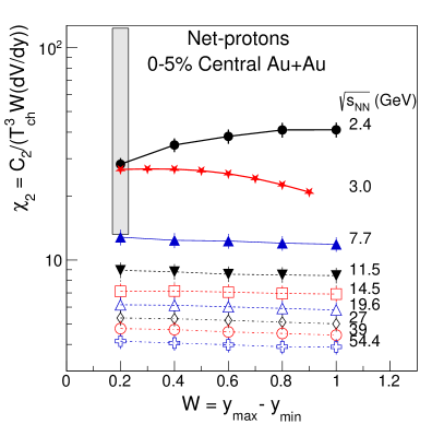
In Table 1 we list , the beam rapidity , and the thermal model parameters extracted from fits to particle yields at each collision energy Adamczewski-Musch et al. (2020); Abdallah et al. (2021, 2023). As and are decreased, more baryons from the incoming nuclei are transported into the central rapidity region, thereby creating systems with a higher . The beam rapidity determines the maximum possible rapidity window () for our analysis. One should avoid subvolumes large enough to contain more than approximately 25% of the total number of protons to minimize baryon number conservation effects Cavagna et al. (2018); Martin et al. (2021); Kuznietsov et al. (2022); Sorensen . This condition is met for most points in our analysis except the wider rapidity bins measured at and 3.0 GeV, where is as large as 0.68. Besides the volume fraction becoming large, there are at least four other challenges to including the 2.4 GeV and 3.0 GeV data in a scaling analysis: 1) The underlying system changes substantially for rapidity windows that span from mid-rapidity to beam rapidity, such as used for the STAR 3.0 GeV data, so that neither nor are approximately constant for the different windows at these energies. 2) While a strong correlation between coordinate space and momentum-space due to the expansion of the collision volume is well understood at 7.7 GeV and above Sorensen (2010); Adamczyk et al. (2016), for lower energies this mapping becomes much more complex so that rapidity windows may not serve as a good proxy for different sizes in coordinate space. 3) The begins changing more rapidly below , whereas from 7.7 GeV to 54.4 GeV, only changes within 10%. 4) For the 2.4 GeV data set, there is ambiguity in the extraction of , , and Motornenko et al. (2021). Here, we take the values extracted by the HADES experiment Adamczewski-Musch et al. (2020), which yield . We find in the literature, however, combinations of parameters that range from 0.46 to 4.3 Motornenko et al. (2021); Chatterjee et al. (2015). The effect of this large ambiguity on is shown with the error band displayed as a shaded gray box in the left panel of Fig. 2. Because of these complications, the 2.4 and 3.0 GeV data are more difficult to interpret than the data at GeV and above.
| (GeV) | (GeV) | (GeV) | () | |
|---|---|---|---|---|
| 2.4 | 0.73 | 0.776 | 0.050 | 17157 |
| 3.0 | 1.05 | 0.720 | 0.080 | 4850 |
| 7.7 | 2.09 | 0.398 | 0.144 | 1044 |
| 11.5 | 2.50 | 0.287 | 0.149 | 1047 |
| 14.5 | 2.73 | 0.264 | 0.152 | 1080 |
| 19.6 | 3.04 | 0.188 | 0.154 | 1137 |
| 27 | 3.36 | 0.144 | 0.155 | 1218 |
| 39 | 3.73 | 0.103 | 0.156 | 1341 |
| 54.4 | 4.06 | 0.083 | 0.160 | 1487 |
The data at 2.4 GeV have been corrected for volume fluctuations. The paper reporting data for 3.0 GeV shows the effect of volume fluctuations based on different models, but refrains from applying a correction because of the observed model dependence. When calculating , we have applied a correction that is the average of the two models, which amounts to scaling the values of for each bin width by 0.88. At the higher energies, the data has been corrected for the centrality bin width, which is shown to be similar to the volume correction in the 0–5% centrality class. For the , data is only published for as a function of the rapidity bin width. Lacking information about as a function of the rapidity bin width, we use the value published for and integrate results, also from STAR STA (2023), to estimate for other rapidity bins and then obtain from .
III Results
In the left panel of Fig. 2, we show the obtained susceptibility as a function of the rapidity bin width for energies ranging from GeV to 54.4 GeV. The errors are the sum of statistical and systematic errors reported in HEPData. All data are from 0–5% central Au+Au collisions. For GeV and above, the data are based on net-proton distributions. For and 3.0 GeV, the production of anti-protons is so rare that only the proton number distributions are needed. As the beam energy increases, decreases and so does the susceptibility. While the higher energies exhibit a slight decrease with increasing , both the and 3.0 GeV data exhibit a less trivial dependence on .
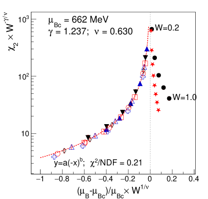
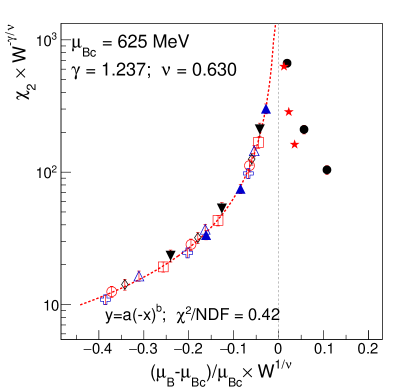
In the right panel of Fig. 2, we show as a function of , where we use the 3-D Ising universality class critical exponents and Sengers and Shanks (2009). After scanning a broad range of values of , we find that the data for collapses on a single curve for MeV. This data collapse provides FSS evidence for the existence of a QCD critical point. We fit the data at to and obtain a best for , . Since FSS is most applicable for data closer to the critical point, we carried out fits both while including all data from 7.7 GeV to 54.4 GeV and with the 39 GeV and 54.4 GeV data excluded. With all data included, we find MeV. With GeV and 54.4 GeV excluded, we find MeV. We also performed fits excluding the wider rapidity bin widths to avoid potential complications from the effects of baryon number conservation as discussed in Sec. I. This also had little effect on the scaling behavior. We note that for the GeV data, the two widest bins still only sample 29% and 36% of the net proton rapidity distribution Vovchenko et al. (2022). Considering that experiments also do not sample the entire transverse momentum distribution, the fraction of the total number of protons that is measured should be small enough for conservation effects to be negligible. We also performed fits using mean-field critical exponents ( and ) which may be more relevant for systems probing the phase diagram further from the critical point. This yielded a good fit with MeV.
Taking all analyses into consideration we estimate the position of the critical point to be MeV. This value is consistent with recent theoretical expectations, including works using Lee-Yang edge singularities Basar (2023), functional renormalization group methods Fu et al. (2020), and a holographic model of QCD Hippert et al. (2023), which yield , , and , respectively. We note, however, that we have not taken scaling with into account. If is far from the values of the data at GeV and above (where ranges from 144 to 160 MeV), then this will create a systematic shift to our extracted .
To estimate the susceptibilities that would be obtained had net-baryons been measured instead of net-protons, we also used the approximate relation obtained in Ref. Kitazawa and Asakawa (2012). In this case, a good scaling requires a much higher value of MeV. We consider this approximate result less robust compared to the scaling based on net-proton data, since any interesting behavior of the system should violate the approximations underlying the correction.
We performed an additional analysis using as the independent variable, and find a good fit with . In this case, the scaled data were fit to with a best for , . Taking the ratio of the two results , we find MeV, which would place the critical temperature about 40 MeV above the chemical freeze-out temperature expected for collisions near MeV, roughly corresponding to GeV. We note that a recent Bayesian analysis of the STAR collective flow data also found evidence for a substantial softening in the equation of state, consistent with a phase transition, near GeV Oliinychenko et al. (2023). This estimate is also slightly higher but within errors of the projection of the lattice QCD pseudo-critical temperature, which would correspond to MeV at Bazavov et al. (2019), though this projection goes beyond the stated range of applicability for lattice calculations.
If the critical point is indeed at MeV, then the GeV and 2.4 GeV data (corresponding to and MeV, respectively) should, ideally, follow a single separate curve at . However, we found that there are no values of which allowed the and 3.0 GeV data to collapse on a common curve with the higher energy data, nor were there any values that brought them into good scaling agreement with each other. This remains true even when exploring a broad range of critical exponents. In Sec. II, we provided several reasons why the and 3.0 GeV data may not be suitable for a FSS analysis. In addition to those, we note that the phase diagram for strongly interacting matter includes an already known critical point for the nuclear liquid-gas phase transition at MeV and MeV Pochodzalla et al. (1995); Elliott et al. (2002); Moretto et al. (2002). Although we often consider the scale of that transition to be too low to affect high energy collisions, it has been shown that the presence of that critical point can modify the expectations for in regions of the phase diagram quite far from the nuclear liquid-gas critical point Vovchenko et al. (2017); Sorensen and Koch (2021); Sorensen et al. (2021). It is plausible that for the GeV data, characterized by and MeV, the nuclear liquid-gas critical point may interfere with the effects of the quark-gluon–plasma—hadronic critical point, spoiling the data collapse. More careful experimental study, including thermal model fits done for yields from specific rapidity windows, publication of as a function of , and more data sets at MeV may help clarify how the data below GeV should be interpreted.
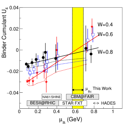
Another method to search for a critical point is to plot the Binder cumulant as a function of for several fixed values of . The curves joining data points measured with the same should cross at , where for any as the correlation length in the continuum limit diverges. In Fig. 3, we show the Binder cumulants as a function of for , 0.6, and 0.8. As mentioned above, for a Gaussian distribution , while for a bimodal or Bernouli distribution ; in the phase coexistence region, one expects a phase separation so that the system becomes more bimodal. At lower , is consistent with a Skellam distribution as expected for a thermal system Braun-Munzinger et al. (2015). For , data is slowly rising as a function of as one would expect when approaching a phase coexistence region. The and 0.6 data are each rising faster, starting systematically below the curve for , crossing over the curve, and ending systematically above the curve for . Linear fits of the and data cross near MeV. The error bars on the data (driven by the uncertainty on ) are rather large, however, the Binder cumulants apparently cross somewhere between and 720 MeV, consistent with our observation of a data collapse for with MeV, shown in the right panel of Fig. 2.
IV Discussion and Caveats
The observation of scaling for and the crossing of in our analysis along with recent theoretical predictions create a cohesive picture pointing to the existence of a critical point in the QCD phase diagram near MeV. There are, however, caveats that may challenge this conclusion. In the discussion of the data collapse for , we pointed out several reasons why the and 3.0 GeV data may not be well-suited to FSS. Even though the Binder cumulants have the advantage that they do not need the thermal model results for or , the other caveats like the potential effects of the nuclear liquid-gas critical point, baryon number conservation, and large variations of the system thermodynamics with still apply to . In addition to the limited statistical precision of , these caveats somewhat weaken the impact of the crossing of , which relies on those very energy points. If we remove the 2.4 and 3.0 GeV from the Binder cumulant analysis, the data from GeV and above seems to suggest the approach to a crossing, but with errors too large for a firm conclusion. Data from the second phase of the STAR Beam Energy Scan should reduce the uncertainties on by roughly a factor of three, helping to clarify whether is consistent with a critical point.
While increasing the precision of the Binder cumulants will be advantageous to this analysis, publishing more data on and as a function of for energies between GeV and 7.7 GeV will be even more helpful in confirming that the data collapse shown in Fig. 2 is truly indicating the presence of a critical point. Experimental collaborations should also extract , , and from particle yields in windows that match the windows for consistent determinations of . Ultimately, model simulations should likewise prove useful in verifying that the heavy-ion data are indeed indicating the presence of a critical point.
V Summary
In this work, we have reported on a finite-size scaling analysis of net-proton number distributions from heavy-ion collisions. We take the rapidity window as the length scale describing the finite size of considered systems, and we use it together with thermal model results on , , and to search for scaling of . We find that data above GeV collapse on a single curve consistent with a critical point at MeV. We also plot Binder cumulants for three fixed values of as a function of and find that the data at different cross in the range of MeV, consistent with a critical point in that range. We argue that this analysis provides convincing evidence for the existence of the QCD critical point near MeV.
We note that, given caveats and uncertainties discussed in the text, one may choose a position of skepticism to a bold discovery claim. It is therefore fortuitous that there will be a wealth of additional data in the near future from the STAR Beam Energy Scan program at RHIC, a planned energy scan with HADES at SIS18, and from the future Compressed Baryonic Matter experiment at FAIR which appears to be situated in an ideal energy range to confirm or refute our findings.
Acknowledgements.
The authors would like to thank Vladimir Skokov, Larry McLerran, and Scott Pratt for insightful comments on the manuscript. P.S. would like to thank Eduardo Fraga and Leticia Palhares for fruitful collaborations on previous FSS analyses. A.S. would like to thank Jacquelyn Noronha-Hostler for providing access to high-performance computing resources, and acknowledges support from the Illinois Campus Cluster, a computing resource that is operated by the Illinois Campus Cluster Program (ICCP) in conjunction with the National Center for Supercomputing Applications (NCSA), which is supported by funds from the University of Illinois at Urbana-Champaign. A.S. further acknowledges support by the U.S. Department of Energy, Office of Science, Office of Nuclear Physics, under Grant No. DE-FG02-00ER41132.Appendix A Supplemental material: Finite-size scaling
Near the critical point of a system in the thermodynamic limit, the dependence of thermodynamic functions can, to the leading order, be expressed through a set of universal power-law relations. It is standard to express these relations using dimensionless variables: the reduced temperature
| (8) |
and reduced chemical potential
| (9) |
where and are the critical temperature and critical chemical potential, respectively. In terms of and , the scaling relations for the specific heat , reduced density , and susceptibility are
| (10) | |||
| (11) | |||
| (12) | |||
| (13) |
where the subscript indicates the continuum limit. These relations define the critical exponents , , , and , and they describe the behavior of the system as a whole (that is, globally) in response to changing and , in particular the divergence of the thermodynamics functions at the critical point. The local response of the system is codified in its correlation function, which depends on the distance between particles , , and whose behavior can can be used to define the correlation length which quantifies the extent of fluctuations in the system. Similarly as the thermodynamic functions, the correlation length in the vicinity of the critical point scales as
| (14) | |||
| (15) |
The above results can be derived within a number of models and are, in fact, universal in the following sense: Not only do the relationships summarized in (10–15) hold in the vicinity of any critical point, but, moreover, the behavior of fundamentally different systems can be categorized into surprisingly few universality classes, characterized by particular values of the critical exponents .
The divergence of thermodynamic functions which is associated with the existence of a critical point, see Eqs. (10–15), occurs only in the thermodynamic limit, i.e., when all dimensions of the considered system approach infinity. If any of the dimensions in the considered problem is finite, the behavior of the thermodynamic functions is correspondingly modified. In particular, for finite systems these divergencies become peaks of finite height, centered around “pseudocritical points” that are shifted with respect to the true critical point.
One of the measures of the “finiteness” of a system is whether the correlation length is comparable to the size of the system, . For many systems, this is equivalent with the requirement that a system is very close to the critical point, where the correlation length diverges and thus reaches macroscopic values. In heavy-ion collisions, however, we are dealing with incredibly small systems (as compared to, for example, a typical sample of a ferromagnetic material); consequently, the correlation length can become comparable with even for systems which are relatively far from the critical point.
In general, one can define three scales associated with a system of finite size: the correlation length , the system size , and the microscopic length which governs the interaction. Any thermodynamic quantities can be then expressed in terms of dimensionless ratios and . In finite-size scaling, one assumes that close to the critical point the microscopic length is of no relevance, leaving and as the only variables of importance. One then explores the hypothesis that a quantity , obtained in the thermodynamic limit, and a quantity , calculated in a finite system characterized by a length scale , can be related to each other by a function dependent on and the infinite-volume correlation length . Assuming, for simplicity, , the above statement can be written as
| (16) |
where is reduced temperature defined using the pseudocritical temperature , that is the temperature at which has a maximum.
To proceed, one starts by assuming that in the thermodynamic limit, the quantity follows a scaling law,
| (17) |
Then one can always consider a particular value of the argument of ,
| (18) |
Given Eq. (14), one can solve Eq. (18) for ,
| (19) |
by means of which Eq. (17) becomes
| (20) |
This in turn transforms Eq. (16) into
| (21) |
so that we get
| (22) |
On the other hand, solving for from Eq. (14), , we can also rewrite Eq. (17) as
| (23) |
Comparing Eqs. (22) and (23) makes it apparent that to obtain the scaling law for the finite-size quantity , one simply needs to substitute the system size for the correlation length . This is intuitive: in the vicinity of the critical point, the correlation length in a finite system is bound by the finite length , so that becomes the relevant scale. Importantly, this upper limit on the size of measured correlations may come both from the physical limitations of the system (a boundary) as well as from the size of a part of the system under consideration (if one of the correlated particles falls outside of the region under consideration, the correlation is not measured and so, for all purposes, it is just as if it doesn’t exist at all).
The proportionality discovered in Eq. (22) can become an equality if we introduce the scaling function , which is taken to be a function of both relevant scales in the system, and ,
| (24) |
Since all the dependence of on is already included in the , it must be that is not proportional to . This can be achieved if is a function of a dimensionless combination of and . Using Eq. (19), one can see that a combination satisfying this requirement is . Therefore,
| (25) |
While the form of is in general not known a priori, one can use Eq. (25) to both uncover this form empirically and find the value of the critical temperature entering the reduced variable . Indeed, one can measure the quantity in systems of varying sizes and plot as a function of . If the value of is not known, one can perform this exercise for a series of proposed values of . Crucially, the plotted points will only fall onto one curve, revealing the shape of the scaling function , for the tested values of approaching the true critical temperature .
Appendix B Supplemental material: Additional results

For FSS, one must characterize the approach to the critical point using an appropriate variable such as . In our simulations, we find good scaling results using . It is not obvious that for heavy-ion collisions data is the correct reduced quantity to carry out scaling. We also investigate as our scaling variable and show a good fit with in Fig. 4.
To address questions about the influence of baryon number conservation, we perform a complementary finite-size scaling analysis using data corresponding to only the smallest three and four rapidity bin widths . Fig. 5 shows the results using , and it is evident that the fit quality remains good. The position of the critical point shifts by only 5 MeV when using the three smallest rapidity bin widths, and remains the same when using four. In our simulations, we find that baryon number conservation only interferes with finite-size scaling when the fraction of baryons used in the cumulant analysis is greater than 25% of the total (see Fig. 1). For collisions at (the data with the narrowest width for the net-proton distribution), the approximate fraction of the total net-proton number for window sizes 0.2, 0.4, 0.6, 0.8, and 1.0, obtained based on the net-proton proton distribution Vovchenko et al. (2022), is 7%, 14%, 22%, 29%, and 36%, respectively. As a result, only the two widest bins at the lowest collider energy exceed the 30% limit. Moreover, this fraction does not take into account the additional loss of protons due to acceptance in and efficiency. As such, it is not likely that conservation effects play a strong role in any of the data used in our fits ( to 54.4 GeV).
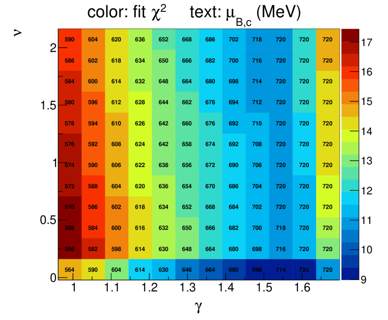
We explored the change in results when using different values of the critical exponents. Whether a system is governed by the 3-D Ising model critical exponents or by mean-field critical exponents depends on the interaction range and on how close one is to the critical point Anisimov et al. (1992). We explored using a range of critical exponents including the mean-field exponents ( and ). Using mean-field exponents we find a good scaling with MeV. We note that even the larger chi-square values in Fig. 6 would represent a good fit, pointing to the need for more data and improved uncertainties to begin to experimentally constrain the critical exponents. We therefore only consider theoretically well-motivated critical exponents in our analysis of the position of the critical point.
References
- Polyakov (1978) A. M. Polyakov, Phys. Lett. B 72, 477 (1978).
- Susskind (1979) L. Susskind, Phys. Rev. D 20, 2610 (1979).
- Collins and Perry (1975) J. C. Collins and M. J. Perry, Phys. Rev. Lett. 34, 1353 (1975).
- Asakawa and Yazaki (1989) M. Asakawa and K. Yazaki, Nucl. Phys. A 504, 668 (1989).
- Braun-Munzinger and Stachel (1996) P. Braun-Munzinger and J. Stachel, Nucl. Phys. A 606, 320 (1996), arXiv:nucl-th/9606017 .
- Fukushima and Sasaki (2013) K. Fukushima and C. Sasaki, Prog. Part. Nucl. Phys. 72, 99 (2013), arXiv:1301.6377 [hep-ph] .
- Sorensen et al. (2024) A. Sorensen et al., Prog. Part. Nucl. Phys. 134, 104080 (2024), arXiv:2301.13253 [nucl-th] .
- Karsch (2002) F. Karsch, Lect. Notes Phys. 583, 209 (2002), arXiv:hep-lat/0106019 .
- Aoki et al. (2006) Y. Aoki, G. Endrodi, Z. Fodor, S. D. Katz, and K. K. Szabo, Nature 443, 675 (2006), arXiv:hep-lat/0611014 .
- Ratti (2018) C. Ratti, Rept. Prog. Phys. 81, 084301 (2018), arXiv:1804.07810 [hep-lat] .
- Barducci et al. (1989) A. Barducci, R. Casalbuoni, S. De Curtis, R. Gatto, and G. Pettini, Phys. Lett. B 231, 463 (1989).
- Halasz et al. (1998) A. M. Halasz, A. D. Jackson, R. E. Shrock, M. A. Stephanov, and J. J. M. Verbaarschot, Phys. Rev. D 58, 096007 (1998), arXiv:hep-ph/9804290 .
- Baym (2002) G. Baym, Nucl. Phys. A 698, XXIII (2002), arXiv:hep-ph/0104138 .
- Allton et al. (2002) C. R. Allton, S. Ejiri, S. J. Hands, O. Kaczmarek, F. Karsch, E. Laermann, C. Schmidt, and L. Scorzato, Phys. Rev. D 66, 074507 (2002), arXiv:hep-lat/0204010 .
- Barbour et al. (1998) I. M. Barbour, S. E. Morrison, E. G. Klepfish, J. B. Kogut, and M.-P. Lombardo, Nucl. Phys. B Proc. Suppl. 60, 220 (1998), arXiv:hep-lat/9705042 .
- Pisarski and Wilczek (1984) R. D. Pisarski and F. Wilczek, Phys. Rev. D 29, 338 (1984).
- Johnson et al. (2023) G. Johnson, F. Rennecke, and V. V. Skokov, Phys. Rev. D 107, 116013 (2023), arXiv:2211.00710 [hep-ph] .
- Rennecke and Skokov (2022) F. Rennecke and V. V. Skokov, Annals Phys. 444, 169010 (2022), arXiv:2203.16651 [hep-ph] .
- Bollweg et al. (2022) D. Bollweg, J. Goswami, O. Kaczmarek, F. Karsch, S. Mukherjee, P. Petreczky, C. Schmidt, and P. Scior (HotQCD), Phys. Rev. D 105, 074511 (2022), arXiv:2202.09184 [hep-lat] .
- Bollweg et al. (2023) D. Bollweg, D. A. Clarke, J. Goswami, O. Kaczmarek, F. Karsch, S. Mukherjee, P. Petreczky, C. Schmidt, and S. Sharma (HotQCD), Phys. Rev. D 108, 014510 (2023), arXiv:2212.09043 [hep-lat] .
- Borsanyi et al. (2020) S. Borsanyi, Z. Fodor, J. N. Guenther, R. Kara, S. D. Katz, P. Parotto, A. Pasztor, C. Ratti, and K. K. Szabo, Phys. Rev. Lett. 125, 052001 (2020), arXiv:2002.02821 [hep-lat] .
- Borsanyi et al. (2022) S. Borsanyi, J. N. Guenther, R. Kara, Z. Fodor, P. Parotto, A. Pasztor, C. Ratti, and K. K. Szabo, Phys. Rev. D 105, 114504 (2022), arXiv:2202.05574 [hep-lat] .
- Mukherjee and Skokov (2021) S. Mukherjee and V. Skokov, Phys. Rev. D 103, L071501 (2021), arXiv:1909.04639 [hep-ph] .
- Connelly et al. (2021) A. Connelly, G. Johnson, S. Mukherjee, and V. Skokov, Nucl. Phys. A 1005, 121834 (2021), arXiv:2004.05095 [hep-ph] .
- Basar (2021) G. Basar, Phys. Rev. Lett. 127, 171603 (2021), arXiv:2105.08080 [hep-th] .
- Dimopoulos et al. (2022) P. Dimopoulos, L. Dini, F. Di Renzo, J. Goswami, G. Nicotra, C. Schmidt, S. Singh, K. Zambello, and F. Ziesché, Phys. Rev. D 105, 034513 (2022), arXiv:2110.15933 [hep-lat] .
- Zambello et al. (2023) K. Zambello, D. A. Clarke, P. Dimopoulos, F. Di Renzo, J. Goswami, G. Nicotra, C. Schmidt, and S. Singh, PoS LATTICE2022, 164 (2023), arXiv:2301.03952 [hep-lat] .
- Schmidt et al. (2023) C. Schmidt, D. A. Clarke, G. Nicotra, F. Di Renzo, P. Dimopoulos, S. Singh, J. Goswami, and K. Zambello, Acta Phys. Polon. Supp. 16, 1 (2023), arXiv:2209.04345 [hep-lat] .
- Aggarwal et al. (2010) M. M. Aggarwal et al. (STAR), (2010), arXiv:1007.2613 [nucl-ex] .
- Odyniec (2019) G. Odyniec (STAR), PoS CORFU2018, 151 (2019).
- Meehan (2016) K. C. Meehan (STAR), Nucl. Phys. A 956, 878 (2016).
- Abdallah et al. (2021) M. Abdallah et al. (STAR), Phys. Rev. C 104, 024902 (2021), arXiv:2101.12413 [nucl-ex] .
- Abdallah et al. (2023) M. Abdallah et al. (STAR), Phys. Rev. C 107, 024908 (2023), arXiv:2209.11940 [nucl-ex] .
- Adamczewski-Musch et al. (2020) J. Adamczewski-Musch et al. (HADES), Phys. Rev. C 102, 024914 (2020), arXiv:2002.08701 [nucl-ex] .
- Ferdinand and Fisher (1969) A. E. Ferdinand and M. E. Fisher, Phys. Rev. 185, 832 (1969).
- Cavagna et al. (2018) A. Cavagna, I. Giardina, and T. S. Grigera, Physics Reports 728, 1 (2018), the physics of flocking: Correlation as a compass from experiments to theory.
- Binder (1981) K. Binder, Zeitschrift für Physik B Condensed Matter 43, 119 (1981).
- Palhares et al. (2011) L. F. Palhares, E. S. Fraga, and T. Kodama, J. Phys. G 38, 085101 (2011), arXiv:0904.4830 [nucl-th] .
- Fraga et al. (2011) E. S. Fraga, L. F. Palhares, and P. Sorensen, Phys. Rev. C 84, 011903 (2011), arXiv:1104.3755 [hep-ph] .
- Lacey et al. (2016) R. A. Lacey, P. Liu, N. Magdy, B. Schweid, and N. N. Ajitanand, (2016), arXiv:1606.08071 [nucl-ex] .
- Martin et al. (2021) D. A. Martin, T. L. Ribeiro, S. A. Cannas, T. S. Grigera, D. Plenz, and D. R. Chialvo, Scientific Reports 11, 15937 (2021).
- Sengers and Shanks (2009) J. V. Sengers and J. G. Shanks, Journal of Statistical Physics 137, 857 (2009).
- Nonaka and Asakawa (2005) C. Nonaka and M. Asakawa, Phys. Rev. C 71, 044904 (2005), arXiv:nucl-th/0410078 .
- Nahrgang et al. (2019) M. Nahrgang, M. Bluhm, T. Schaefer, and S. A. Bass, Phys. Rev. D 99, 116015 (2019), arXiv:1804.05728 [nucl-th] .
- Stephanov and Yin (2018) M. Stephanov and Y. Yin, Phys. Rev. D 98, 036006 (2018), arXiv:1712.10305 [nucl-th] .
- Sorensen and Koch (2021) A. Sorensen and V. Koch, Phys. Rev. C 104, 034904 (2021), arXiv:2011.06635 [nucl-th] .
- Vovchenko et al. (2020) V. Vovchenko, O. Savchuk, R. V. Poberezhnyuk, M. I. Gorenstein, and V. Koch, Phys. Lett. B 811, 135868 (2020), arXiv:2003.13905 [hep-ph] .
- Kuznietsov et al. (2022) V. A. Kuznietsov, O. Savchuk, M. I. Gorenstein, V. Koch, and V. Vovchenko, Phys. Rev. C 105, 044903 (2022), arXiv:2201.08486 [hep-ph] .
- Hatta and Stephanov (2003) Y. Hatta and M. A. Stephanov, Phys. Rev. Lett. 91, 102003 (2003), [Erratum: Phys.Rev.Lett. 91, 129901 (2003)], arXiv:hep-ph/0302002 .
- Kitazawa and Asakawa (2012) M. Kitazawa and M. Asakawa, Phys. Rev. C 85, 021901 (2012), arXiv:1107.2755 [nucl-th] .
- Fukugita et al. (1990) M. Fukugita, H. Mino, M. Okawa, and A. Ukawa, Phys. Rev. Lett. 65, 816 (1990).
- Karsch et al. (2001) F. Karsch, E. Laermann, and C. Schmidt, Phys. Lett. B 520, 41 (2001), arXiv:hep-lat/0107020 .
- Andronic et al. (2018) A. Andronic, P. Braun-Munzinger, K. Redlich, and J. Stachel, Nature 561, 321 (2018), arXiv:1710.09425 [nucl-th] .
- STA (2023) (2023), arXiv:2311.11020 [nucl-ex] .
- (55) A. Sorensen, in preparation.
- Sorensen (2010) P. Sorensen, “Elliptic Flow: A Study of Space-Momentum Correlations In Relativistic Nuclear Collisions,” in Quark-gluon plasma 4, edited by R. C. Hwa and X.-N. Wang (2010) pp. 323–374, arXiv:0905.0174 [nucl-ex] .
- Adamczyk et al. (2016) L. Adamczyk et al. (STAR), Phys. Rev. Lett. 116, 112302 (2016), arXiv:1601.01999 [nucl-ex] .
- Motornenko et al. (2021) A. Motornenko, J. Steinheimer, V. Vovchenko, R. Stock, and H. Stoecker, Phys. Lett. B 822, 136703 (2021), arXiv:2104.06036 [hep-ph] .
- Chatterjee et al. (2015) S. Chatterjee, S. Das, L. Kumar, D. Mishra, B. Mohanty, R. Sahoo, and N. Sharma, Adv. High Energy Phys. 2015, 349013 (2015).
- Vovchenko et al. (2022) V. Vovchenko, V. Koch, and C. Shen, Phys. Rev. C 105, 014904 (2022), arXiv:2107.00163 [hep-ph] .
- Basar (2023) G. Basar, (2023), arXiv:2312.06952 [hep-th] .
- Fu et al. (2020) W.-j. Fu, J. M. Pawlowski, and F. Rennecke, Phys. Rev. D 101, 054032 (2020), arXiv:1909.02991 [hep-ph] .
- Hippert et al. (2023) M. Hippert, J. Grefa, T. A. Manning, J. Noronha, J. Noronha-Hostler, I. Portillo Vazquez, C. Ratti, R. Rougemont, and M. Trujillo, (2023), arXiv:2309.00579 [nucl-th] .
- Oliinychenko et al. (2023) D. Oliinychenko, A. Sorensen, V. Koch, and L. McLerran, Phys. Rev. C 108, 034908 (2023), arXiv:2208.11996 [nucl-th] .
- Bazavov et al. (2019) A. Bazavov et al. (HotQCD), Phys. Lett. B 795, 15 (2019), arXiv:1812.08235 [hep-lat] .
- Pochodzalla et al. (1995) J. Pochodzalla et al., Phys. Rev. Lett. 75, 1040 (1995).
- Elliott et al. (2002) J. B. Elliott et al. (ISiS), Phys. Rev. Lett. 88, 042701 (2002), arXiv:nucl-ex/0104013 .
- Moretto et al. (2002) L. G. Moretto, J. B. Elliott, L. Phair, G. J. Wozniak, C. M. Mader, and A. Chappars, AIP Conf. Proc. 610, 182 (2002).
- Vovchenko et al. (2017) V. Vovchenko, M. I. Gorenstein, and H. Stoecker, Phys. Rev. Lett. 118, 182301 (2017), arXiv:1609.03975 [hep-ph] .
- Sorensen et al. (2021) A. Sorensen, D. Oliinychenko, V. Koch, and L. McLerran, Phys. Rev. Lett. 127, 042303 (2021), arXiv:2103.07365 [nucl-th] .
- Braun-Munzinger et al. (2015) P. Braun-Munzinger, A. Kalweit, K. Redlich, and J. Stachel, Phys. Lett. B 747, 292 (2015), arXiv:1412.8614 [hep-ph] .
- Anisimov et al. (1992) M. Anisimov, S. Kiselev, J. Sengers, and S. Tang, Physica A: Statistical Mechanics and its Applications 188, 487 (1992).