Quadratic quasi-normal mode dependence on linear mode parity

Abstract

Quasi-normal modes (QNMs) uniquely describe the gravitational-wave ringdown of post-merger black holes. While the linear QNM regime has been extensively studied, recent work has highlighted the importance of second-perturbative-order, quadratic QNMs (QQNMs) arising from the nonlinear coupling of linear QNMs. Previous attempts to quantify the magnitude of these QQNMs have shown discrepant results. Using a new hyperboloidal framework, we resolve the discrepancy by showing that the QQNM/QNM ratio is a function not only of the black hole parameters but also of the ratio between even- and odd-parity linear QNMs: the ratio QQNM/QNM depends on what created the ringing black hole, but only through this ratio of even- to odd-parity linear perturbations.

Introduction.—After the merger of two black holes (BHs), the distorted remnant BH rings down towards a stationary state through its emission of gravitational waves (GWs). The signal associated with this process is well modelled by a superposition of exponentially damped sinusoids, with complex frequencies given by the so-called quasi-normal modes (QNMs) [1, 2, 3, 4]. For an isolated system within General Relativity (GR), these QNM frequencies are uniquely determined by the mass and spin of the final BH. Each frequency $\omega_{\ell\mathtt{m}\mathtt{n}}$ is characterised by three integers: polar and azimuthal indices $(\ell,\mathtt{m})$ associated with a projection onto spherical harmonics on the celestial sphere, and an overtone index $n=0,1,\ldots$ that enumerates the frequencies for a given angular mode.

Inspired by the uniqueness of the QNM spectrum, the BH spectroscopy program [5, 6, 7] aims at extracting multiple QNMs from ringdown signals in order to perform stringent tests of GR, probe the BH geometry, and constrain features of the surrounding environment [1, 2, 3]. Measurements of the dominant QNM, $(\ell,\mathtt{m},\mathtt{n})=(2,\pm 2,0)$, in GW signals are well established [8, 9, 10]. The detection of higher overtones and higher angular modes is still under debate [11, 12, 13, 14, 15, 16, 17, 18, 19, 20, 21, 22, 23, 24], but future GW detectors such as the Einstein Telescope and LISA are expected to observe these higher modes regularly. Current forecasts predict $20-50$ events per year with at least two detectable QNMs for stellar-mass binaries [25, 26] and even $\sim 5-8$ QNMs for massive BH binaries with LISA [7, 27].

Historically, the BH spectroscopy program has been entirely based on linear BH perturbation theory (BHPT) [1, 2, 3, 4, 5, 6], and forecasts for future QNM detections assume only linear QNM frequencies. However, GR is a nonlinear theory, and recent milestone results have shown that BH spectroscopy must also account for second-order, quadratic perturbations, which can dominate over linear overtones [28, 29, 30, 31, 20, 32, 33, 34]. In these quadratic perturbations, a new set of characteristic frequencies arises: the so-called quadratic QNMs (QQNMs) $\omega_{\ell_{1}\mathtt{m}_{1}\mathtt{n}_{1}\times\ell_{2}\mathtt{m}_{2}\mathtt{n}_{2}}=\omega_{\ell_{1}\mathtt{m}_{1}\mathtt{n}_{1}}+\omega_{\ell_{2}\mathtt{m}_{2}\mathtt{n}_{2}}$, which result from the coupling of two linear QNMs. A recent analysis indicates that the Einstein Telescope and Cosmic Explorer could detect QQNMs in up to a few tens of events per year [35]. While the predictions for LISA depend sensitively on the astrophysical massive BH formation models, the most optimistic scenario allows for up to ${\cal O}(1000)$ events with detectable QQNMs in LISA’s nominal 4-year observation time [35].

Spurred by these developments, there has been a spate of recent work devoted to analysing QQNMs and their impact on BH spectroscopy. Most calculations have been based on extracting modes from fully nonlinear numerical relativity (NR) simulations of BH binary evolutions, but a number of recent calculations have also been performed using second-order BHPT [34, 36, 37]. These calculations have generally focused on a single measure of the significance of QQNMs: the ratio between a given QQNM mode amplitude and the amplitude(s) of the linear parent mode(s) that generate it. Perhaps surprisingly, different analyses have led to conflicting values of the ratio, even in the simplest case of non-rotating BHs.

It has been suggested that the discrepancies in Schwarzschild could be due to the freedom to excite both even- and odd-parity perturbations [34]. We find that this can explain the discrepancy in previous QQNM analyses, but this property is not restricted to a Schwarzschild background; it also holds in Kerr. Consequently, we observe that reported QQNM/QNM ratios in the literature often lack sufficient information to describe the relationship between linear and non-linear QNMs fully. To shift this paradigm, we establish that the ratio depends not only on the BH parameters, but also on the properties of the system that created the ringing BH. Specifically, it is a function of the ratio between the amplitudes of even- and odd-parity linear QNMs; this ratio will depend on the degree to which the progenitor system possessed equatorial (up-down) symmetry.

As a proof of principle, we make this argument precise, and present numerical results for the QQNM/QNM ratio, in the simple case of Schwarzschild spacetime. We discuss the generalisation to the most generic case in the conclusion. Our calculation utilizes a novel code combining two critical components: a hyperboloidal frequency-domain framework that allows us to directly and accurately compute the physical waveform without requiring regularization [38, 39, 40, 41, 42, 43, 44, 45]; and a covariant second-order BHPT formalism [46, 47]. By controlling the geometrical aspects of the problem and using the mode-coupling tools of Ref. [46], we are able to fine-tune the first-order dynamics to single out any number of linear modes and obtain the quadratic contribution from the linear even- and odd-parity sectors semi-analytically.

Black hole perturbation theory.—In BHPT we expand the spacetime metric in the form $g_{ab}+\varepsilon h^{(1)}_{ab}+\varepsilon^{2}h^{(2)}_{ab}+\ldots$, where $g_{ab}$ is a Kerr metric and $\varepsilon=1$ counts perturbative orders. In vacuum, the perturbations satisfy the Einstein equations

$$\varepsilon\delta G_{ab}[h^{(1)}_{cd}]+\varepsilon^{2}\bigl{(}\delta G_{ab}[h^{(2)}_{cd}]+\delta^{2}G_{ab}[h^{(1)}_{cd}]\bigr{)}+\ldots=0,$$ (1)

where $\delta G_{ab}$ is the linearized Einstein tensor and $\delta^{2}G_{ab}[h^{(1)}_{cd}]$ is quadratic in $h^{(1)}_{cd}$ [48].

At linear order all nontrivial information in $h^{(1)}_{ab}$ is encoded in the linearized Weyl scalar $\Psi^{(1)}_{4}$, which satisfies the vacuum Teukolsky equation ${\mathcal{O}}[\Psi_{4}^{(1)}]=0$, where ${\mathcal{O}}$ is a linear second-order differential operator [49, 50].

We adopt compactified hyperboloidal coordinates $(\tau,\sigma,\theta,\varphi)$ [42, 39], in which constant-$\tau$ slices connect the future horizon $\mathscr{H}^{+}$ (at compactified radial coordinate $\sigma=1$) to future null infinity $\mathscr{I}^{+}$ (at $\sigma=0$). Using the hyperboloidal time $\tau$, we introduce the frequency-domain field ${\psi}_{4}^{(1)}$ via a Laplace (or Fourier) transform,

$$\psi_{4}^{(1)}(\sigma,\theta,\varphi;s)=\int_{0}^{\infty}{\Psi}_{4}^{(1)}(\tau,\sigma,\theta,\varphi)e^{-s\tau}d\tau.$$ (2)

The complex Laplace parameter $s$ is related to the usual complex frequency $\omega$ by $s=-i\omega$. We next separate the Teukolsky equation into an angular and radial part by decomposing $\psi_{4}^{(1)}$ into spin-weighted spheroidal harmonics [49, 50, 51],

$$\psi_{4}^{(1)}=\mathcal{Z}(\sigma)\sum_{\ell\mathtt{m}}\tilde{\psi}_{\ell\mathtt{m}}^{(1)}(\sigma;s){}_{-2}S_{\ell\mathtt{m}}(\theta,\varphi;s).$$ (3)

Here $\mathcal{Z}(\sigma)$ serves to factor out the dominant behavior near $\mathscr{H}^{+}$ and $\mathscr{I}^{+}$; a linear vacuum perturbation $\Psi^{(1)}_{4}$ scales quadratically with distance from the horizon near $\mathscr{H}^{+}$ and decays inversely with distance toward $\mathscr{I}^{+}$ [42, 48], motivating us to choose $\mathcal{Z}(\sigma)\propto\sigma(1-\sigma)^{2}$. Because we use hyperboloidal slices [52, 42, 44], the modes $\tilde{\psi}_{\ell\mathtt{m}}^{(1)}$ are smooth on the entire domain, $\sigma\in[0,1]$, and because we factor out $\mathcal{Z}$ we can directly compute the waveform from $\tilde{\psi}_{\ell\mathtt{m}}^{(1)}$ at $\sigma=0$.

The Laplace transform and spheroidal-harmonic expansion leaves us with a radial Teukolsky equation, $\mathcal{D}_{\ell\mathtt{m}}[\tilde{\psi}_{\ell\mathtt{m}}^{(1)}(\sigma;s)]=0$, where $\mathcal{D}_{\ell\mathtt{m}}$ is a linear second-order radial operator. In the hyperboloidal setup, linear QNMs are the solutions to this equation that satisfy regularity conditions at both ends ($\sigma=0$ and 1). Such solutions only exist for the countable set of QNM frequencies $s_{\ell\mathtt{m}\mathtt{n}}$, and we denote them $\tilde{\psi}_{\ell\mathtt{m}\mathtt{n}}^{(1)}(\sigma):=\tilde{\psi}_{\ell\mathtt{m}}^{(1)}(\sigma;s_{\ell\mathtt{m}\mathtt{n}})$.

Given a set of QNM solutions, $\tilde{\psi}^{(1)}_{\ell\mathtt{m}\mathtt{n}}$, the inverse Laplace transform yields a time-domain solution of the form [39]

$$\Psi_{4}^{(1)}=\mathcal{Z}(\sigma)\sum_{\ell\mathtt{m}\mathtt{n}}A_{\ell\mathtt{m}\mathtt{n}}\tilde{\psi}_{\ell\mathtt{m}\mathtt{n}}^{(1)}(\sigma)e^{s_{\ell\mathtt{m}\mathtt{n}}\tau}{}_{-2}S_{\ell\mathtt{m}}(\theta,\varphi;s_{\ell\mathtt{m}\mathtt{n}}).$$ (4)

Since QNM solutions are only defined up to an overall constant factor, the $A_{\ell\mathtt{m}\mathtt{n}}$ are arbitrary (complex) excitation coefficients, and we set $\tilde{\psi}_{\ell\mathtt{m}\mathtt{n}}^{(1)}=1$ at $\mathscr{I}^{+}$. In Eq. (4), we neglect late-time tail contributions that generically arise [53]; this choice fixes a pure QNM dynamics at linear order.

Mirror modes and parity.—The azimuthal symmetry of Kerr spacetime causes a symmetry between the $+\mathtt{m}$ and $-\mathtt{m}$ QNM frequencies [51, 54]

$$s_{\ell-\mathtt{m}n}=s_{\ell\mathtt{m}n}^{*}.$$ (5)

Additionally, our choice of normalization implies that the corresponding eigenfunctions are related by $\tilde{\psi}_{\ell-\mathtt{m}\mathtt{n}}=\tilde{\psi}_{\ell\mathtt{m}\mathtt{n}}^{\star}$. The QNMs with $\mathtt{m}\geq 0$ and $\mathtt{m}<0$ are known as the regular and mirror QNMs, respectively. They decay at the same rate but oscillate in opposite directions.

In Schwarzschild spacetime, the frequencies degenerate: prograde and retrograde modes become indistinguishable and $\mathtt{m}$-independent. Nonetheless, QNM frequencies come in complex conjugate pairs, and the full solution can still be written in the form of (4), where one can impose (without loss of generality) the mirror relation in (5).

Most QNM analyses have exclusively considered the regular QNMs. In [54], the importance of including mirror QNMs was demonstrated in linear QNM analyses to reduce systematic uncertainties. In this work, we find that mirror modes also play a crucial role in QQNM analysis.

The ratio between regular and mirror modes, $A_{\ell-\mathtt{m}\mathtt{n}}/A_{\ell\mathtt{m}\mathtt{n}}$, is directly related to the ratio between even- and odd-parity contributions to the GW. At $\mathscr{I}^{+}$, the GW (or more strictly, the shear [55]) can be naturally decomposed into even-parity ($Y_{AB}$) and odd-parity ($X_{AB}$) tensor harmonics [56, 46],

$$h_{AB}^{(1)}=r^{2}\mathcal{Z}(\sigma)\sum_{\ell\mathtt{m}\mathtt{n}}\left(C^{+}_{\ell\mathtt{m}\mathtt{n}}Y_{AB}^{\ell\mathtt{m}}+C^{-}_{\ell\mathtt{m}\mathtt{n}}X_{AB}^{\ell\mathtt{m}}\right)e^{s_{\ell\mathtt{m}\mathtt{n}}\tau},$$ (6)

where it is understood that this applies in the $r\to\infty$ ($\sigma\to 0$) limit, $\theta^{A}=(\theta,\varphi)$, the factor of $r^{2}$ corresponds to the natural scaling of angular components, $C_{\pm}^{\ell\mathtt{m}\mathtt{n}}$ are constant (complex) amplitudes, and $\tau=u$ (the usual outgoing null coordinate).

For comparison, $\Psi_{4}^{(1)}$ at $\mathscr{I}^{+}$ can be decomposed into the closely-related spin-weight $-2$ spherical harmonics ${}_{-2}Y_{\ell\mathtt{m}}$ (requiring a projection from spheroidal harmonics, except in the Schwarzschild case where ${}_{-2}S_{\ell\mathtt{m}}$ reduces to ${}_{-2}Y_{\ell\mathtt{m}}$). To relate the amplitudes $A_{\ell\mathtt{m}\mathtt{n}}$ to $C^{\ell\mathtt{m}}_{\pm}$, we use the relations between harmonics in Ref. [46] together with the fact that $\lim_{r\rightarrow\infty}\Psi_{4}^{(1)}=-\frac{1}{2}\lim_{r\rightarrow\infty}\ddot{h}_{\bar{m}\bar{m}}$, where $\bar{m}^{A}=\frac{1}{\sqrt{2}r}(1,i\csc\theta)$. A short calculation reveals

$$A_{\ell\mathtt{m}\mathtt{n}} =-\frac{s_{\ell\mathtt{m}\mathtt{n}}^{2}}{4}\lambda_{\ell,2}\left(C^{+}_{\ell\mathtt{m}\mathtt{n}}-iC^{-}_{\ell\mathtt{m}\mathtt{n}}\right),$$ (7)

$$A_{\ell-\mathtt{m}\mathtt{n}}^{\star} =-(-1)^{\mathtt{m}}\frac{s_{\ell\mathtt{m}\mathtt{n}}^{2}}{4}\lambda_{\ell,2}\left(C^{+}_{\ell\mathtt{m}\mathtt{n}}+iC^{-}_{\ell\mathtt{m}\mathtt{n}}\right),$$ (8)

where $\lambda_{\ell,2}=\sqrt{(\ell+2)!/(\ell-2)!}$. Equation (8) follows from the mirror relation (5) and the fact that the 4D metric perturbation is real, i.e., $C^{\pm}_{\ell-\mathtt{m}\mathtt{n}}=(-1)^{m}(C^{\pm}_{\ell\mathtt{m}\mathtt{n}})^{\star}$.

Equations (7) and (8) imply that the complex ratio $A_{\ell-\mathtt{m}\mathtt{n}}/A_{\ell\mathtt{m}\mathtt{n}}$ is a simple function of $C_{\ell\mathtt{m}\mathtt{n}}^{-}/C_{\ell\mathtt{m}\mathtt{n}}^{+}$. We emphasize that while it is impossible to omit $\mathtt{m}<0$ modes from $h^{(1)}_{AB}$ (as they are required for $h^{(1)}_{AB}$ to be real-valued), it is possible to omit $\mathtt{m}<0$ modes in $\Psi^{(1)}_{4}$; this corresponds to the particular ratio $C^{+}_{\ell\mathtt{m}\mathtt{n}}=-iC_{\ell\mathtt{m}\mathtt{n}}^{-}$.

Quadratic QNMs.—Like at first order, the second-order contribution to the GW is fully encoded in a linear Weyl scalar $\Psi_{4L}^{(2)}$ constructed from $h^{(2)}_{ab}$ [57, 47]. $\Psi_{4L}^{(2)}$ satisfies a “reduced” second-order Teukolsky equation derived from the second-order terms in the Einstein equation (1) [58, 47]:

$${\mathcal{O}}[\Psi_{4L}^{(2)}]=-{\mathcal{S}}[\delta^{2}G_{ab}[h^{(1)}_{cd}]]:=\tilde{\mathcal{S}},$$ (9)

where ${\mathcal{S}}$ is a linear second-order differential operator [48].

The source in Eq. 9 depends quadratically on the first-order metric perturbation; schematically,

$$\tilde{\mathcal{S}}\sim\nabla\nabla(\nabla h^{(1)}_{ab})^{2}\;.$$ (10)

In Schwarzschild [46], the $\ell\mathtt{m}$ modes of $\tilde{\mathcal{S}}$ are readily computed from an arbitrary set of first-order $\ell\mathtt{m}$ modes using the Mathematica package PerturbationEquations [59].

We obtain the $\ell\mathtt{m}$ modes of $h^{(1)}_{ab}$ using a standard metric reconstruction procedure [48] in the outgoing radiation gauge (ORG), in which $h^{(1)}_{ab}$ is computed from a Hertz potential $\Phi^{\rm ORG}$ satisfying the inversion relation

$$\Psi_{4}^{(1)} =\frac{1}{4}\hbox{\ec\char 222\relax}^{\prime 4}\bar{\Phi}^{\rm ORG},$$ (11)

where $\hbox{\ec\char 222\relax}^{\prime}$ is a derivative along ingoing principal null rays [48]. In terms of this Hertz potential,

$$h_{ab}^{(1)} =2\mathrm{Re}({\mathcal{S}}^{\dagger}\Phi^{\rm ORG})_{ab},$$ (12)

where ${\mathcal{S}}^{\dagger}$ denotes the adjoint of ${\mathcal{S}}$.

Note that $h^{(1)}_{ab}$ depends on both $\Phi^{\rm ORG}$ and $\bar{\Phi}^{\rm ORG}$ and therefore on both $\Psi_{4}$ and $\bar{\Psi}_{4}$ via Eq. 11. Consequently, each QQNM amplitude depends on regular and mirror linear QNM amplitudes. To elucidate this, we consider $\Psi_{4}^{(1)}$ being composed of a single regular and mirror mode in Schwarzschild spacetime,

$$\Psi^{(1)}_{4}=\mathcal{Z}(\sigma)\Bigl{\{}A_{\ell\mathtt{m}\mathtt{n}}\tilde{\psi}_{\ell\mathtt{m}\mathtt{n}}^{(1)}(\sigma)e^{s_{\ell\mathtt{m}\mathtt{n}}\tau}{}_{-2}Y_{\ell\mathtt{m}}(\theta,\phi)$$

$$+A_{\ell-\mathtt{m}\mathtt{n}}(\tilde{\psi}_{\ell\mathtt{m}\mathtt{n}}^{(1)}(\sigma))^{\star}e^{s_{\ell\mathtt{m}\mathtt{n}}^{\star}\tau}{}_{-2}Y_{\ell-\mathtt{m}}(\theta,\phi)\Bigr{\}}.$$ (13)

Equations (10)–(12) show that the second-order source $\tilde{\mathcal{S}}$ depends quadratically on $\Psi^{(1)}_{4}$ and $\bar{\Psi}^{(1)}_{4}$. Via our ansatz (Quadratic quasi-normal mode dependence on linear mode parity) and Eq. 5, $\tilde{\mathcal{S}}$ is hence composed of three distinct terms,

$$\tilde{\mathcal{S}}=\mathcal{Z}(\sigma)\Bigl{\{} \tilde{S}^{LM}(\sigma)e^{2s_{\ell\mathtt{m}\mathtt{n}}\tau}{}_{-2}Y_{LM}(\theta,\phi)$$

$$+\tilde{S}^{L0}(\sigma)e^{2{\rm Re}(s_{\ell\mathtt{m}\mathtt{n}})\tau}{}_{-2}Y_{L0}(\theta,\phi)$$

$$+\tilde{S}^{L-M}(\sigma)e^{2s_{\ell\mathtt{m}\mathtt{n}}^{\star}\tau}{}_{-2}Y_{L-M}(\theta,\phi)\Bigr{\}},$$ (14)

where $L=2\ell$, and $M=2\mathtt{m}$.

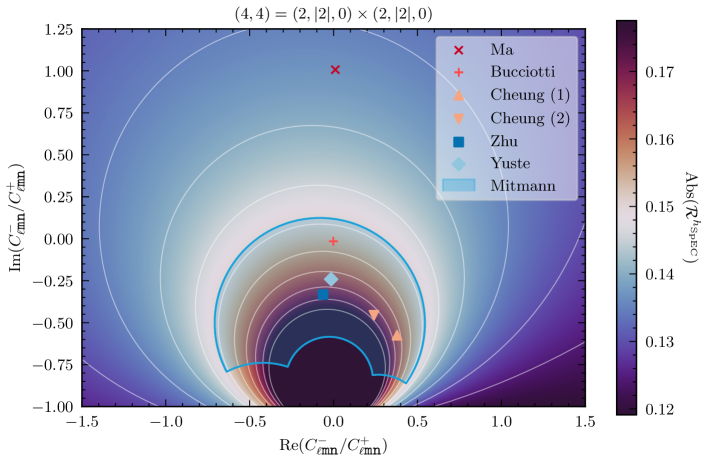
Figure 1: Contour plot of the ratio $\left(\mathcal{R}^{h_{\rm{SpEC}}}\right)^{LM}_{(\ell\mathtt{m}\mathtt{n})\times(\ell\mathtt{m}\mathtt{n})}$ as a function of the odd-to-even complex amplitude ratio $C_{-}^{\ell\mathtt{m}\mathtt{n}}/C_{+}^{\ell\mathtt{m}\mathtt{n}}$ for the quadratic mode $(4,4)=(2,|2|,0)\times(2,|2|,0)$. The solid lines are values of constant amplitude of the QQNM ratio. We have also indicated previous results in the literature: Ma et al. (dark red cross) [34]; Bucciotti et al. (light red plus) [37]; Cheung et al. (orange triangle) [28]; Cheung et al. (inverted orange triangle) [33]; Zhu et al. (dark blue square) [36]; Redondo-Yuste et al. (light blue diamond) [32]; and Mitmann et al. (light blue region) [29]. Since, the result given in Mitmann et al [29] is for a range of values for the magnitude and phase of the QQNM ratio, we have therefore plotted this as a region in the contour plot.

Given the source (Quadratic quasi-normal mode dependence on linear mode parity), we solve Eq. (9) following the same procedure as at first order, performing a Laplace transform in hyperboloidal time, decomposing into $\ell\mathtt{m}$ modes, and solving the resulting radial equations. The time-domain solution is obtained by applying an inverse Laplace transform, which contains the same modes as the source (Quadratic quasi-normal mode dependence on linear mode parity) (in addition to tails and other contributions that we neglect). In particular, it is composed of $(L,M),(L,0),(L,-M)$ spherical modes, with associated frequencies $2s_{\ell\mathtt{m}\mathtt{n}}$, $2{\rm Re}(s_{\ell\mathtt{m}\mathtt{n}})$ and $2s_{\ell\mathtt{m}\mathtt{n}}^{\star}$. Each of these QQNMs depends on the first-order excitation coefficients in the following way:

$$\left(\Psi_{4L}^{(2)}\right)^{LM} =a^{LM}(\sigma)A_{\ell\mathtt{m}\mathtt{n}}^{2}+b^{LM}(\sigma)A_{\ell\mathtt{m}\mathtt{n}}A_{\ell-\mathtt{m}\mathtt{n}}^{\star},$$ (15)

$$\left(\Psi_{4L}^{(2)}\right)^{L0} =a^{L0}(\sigma)A_{\ell\mathtt{m}\mathtt{n}}A_{\ell-\mathtt{m}\mathtt{n}}+b^{L0}(\sigma)A_{\ell\mathtt{m}\mathtt{n}}A_{\ell\mathtt{m}\mathtt{n}}^{\star}$$

$$\quad+\left(b^{L0}(\sigma)\right)^{\star}A_{\ell-\mathtt{m}\mathtt{n}}A_{\ell-\mathtt{m}\mathtt{n}}^{\star},$$ (16)

$$\left(\Psi_{4L}^{(2)}\right)^{L-M} =\left(a^{LM}(\sigma)\right)^{\star}A_{\ell-\mathtt{m}\mathtt{n}}^{2}+\left(b^{LM}(\sigma)\right)^{\star}A_{\ell\mathtt{m}\mathtt{n}}^{\star}A_{\ell-\mathtt{m}\mathtt{n}}.$$ (17)

We provide the coefficients ($a^{LM}$ etc.), evaluated at $\mathscr{I}^{+}$, in the Supplemental Material.

Note that one can uniquely determine the two excitation amplitudes of the first-order data, $A_{\ell\mathtt{m}\mathtt{n}}$ and $A_{\ell-\mathtt{m}\mathtt{n}}$, up to an overall sign, from the excitations at second order, by solving the system (15)–(17) for $A_{\ell\mathtt{m}\mathtt{n}}$ and $A_{\ell-\mathtt{m}\mathtt{n}}$ at a radial point $\sigma=\sigma_{0}$, for example at $\mathscr{I}^{+}$, $\sigma_{0}=0$. Given the relations (7)–(8), this means that from the QQNMs one can uniquely determine, up to an overall sign (which corresponds to a phase difference of $+\pi$), the contribution of the even and odd sectors of the first-order QNMs. The residual sign ambiguity is due to the fact that the second-order source, and therefore the QQNMs, are invariant under a sign change $\Psi_{4}^{(1)}\to-\Psi_{4}^{(1)}$; see again Eq. (10).

Results.—We specialise to the scenario described above, with first-order pure QNM data consisting of a single regular and mirror mode, as in (Quadratic quasi-normal mode dependence on linear mode parity). The ensuing nonzero pieces of the second-order Weyl scalar are of the form (15)–(17). For concreteness, we display results for the QQNM mode with frequency $2s_{\ell\mathtt{m}\mathtt{n}}$, which corresponds to the expression in Eq. (15).

Typically, one is not directly interested in the value of $\left(\Psi_{4L}^{(2)}\right)^{LM}$ at $\mathscr{I}^{+}$, but in how it compares to the first-order perturbation. Since $\Psi_{4L}^{(2)}\sim\bigl{(}\Psi_{4}^{(1)}\bigr{)}^{2}$, we might consider the following ratio:

$$\left(\mathcal{R}^{\Psi_{4}}\right)^{LM}:=\frac{\left(\Psi_{4L}^{(2)}\right)^{LM}}{A_{\ell\mathtt{m}\mathtt{n}}^{2}}.$$ (18)

However, for comparison with the literature, it is more convenient to define the analogous ratio from the strain $h$, related to the Weyl scalar by $\Psi_{4}\sim\ddot{h}$. Employing the SpEC conventions (which notably use a re-scaled Kinnersley tetrad) [36], we arrive at the relation

$$\left(\mathcal{R}^{h_{\rm{SpEC}}}\right)^{LM}=-s_{\ell\mathtt{m}\mathtt{n}}^{2}\left(\mathcal{R}^{\Psi_{4}}\right)^{LM}.$$ (19)

Note that, apart from numerical factors, these ratios only depend on the ratio between mirror and regular mode amplitudes, $A_{\ell-\mathtt{m}\mathtt{n}}^{\star}/A_{\ell\mathtt{m}\mathtt{n}}$. For example, $\left(\mathcal{R}^{\Psi_{4}}\right)^{LM}=a^{LM}(0)+b^{LM}(0)A_{\ell-\mathtt{m}\mathtt{n}}^{\star}/A_{\ell\mathtt{m}\mathtt{n}}$. Using Eqs. (7) and (8), we can alternatively express $\left(\mathcal{R}^{\Psi_{4}}\right)^{LM}$ in terms of the ratio of odd to even amplitudes, $C^{-}_{\ell\mathtt{m}\mathtt{n}}/C^{+}_{\ell\mathtt{m}\mathtt{n}}$. In Kerr spacetime $\left(\mathcal{R}^{\Psi_{4}}\right)^{LM}$ is also a function of the BH parameters and $C^{-}_{\ell\mathtt{m}\mathtt{n}}/C^{+}_{\ell\mathtt{m}\mathtt{n}}$. This can be derived by inputting Eq. (12) into the expression for the source, $\tilde{\mathcal{S}}$, available in Ref. [60]. This shows that the source consists of terms $\propto\bar{\Phi}^{2}$ and $\propto\Phi\bar{\Phi}$. Hence, using Eqs. (11), (Quadratic quasi-normal mode dependence on linear mode parity), and (5), similar relations as Eqs. (15) to (17) hold in Kerr (up to angular mode mixing) and $\left(\mathcal{R}^{\Psi_{4}}\right)^{LM}$ is a function of $C^{-}_{\ell\mathtt{m}\mathtt{n}}/C^{+}_{\ell\mathtt{m}\mathtt{n}}$ and the BH parameters.

In Fig. 1, we show a contour plot of $\left(\mathcal{R}^{h_{\rm{SpEC}}}\right)^{LM}$ as a function of $C^{-}_{\ell\mathtt{m}\mathtt{n}}/C^{+}_{\ell\mathtt{m}\mathtt{n}}$ for the case $(\ell,\mathtt{m},\mathtt{n})=(2,2,0)$. We also include previous results from the literature in this plot. We relegate to the Supplemental Material how the data points were added to the figure. Notably, one should distinguish the results reported by Ma et al. [34] (dark red cross), which differ significantly from NR results (in blue and orange), and from the BHPT result reported by Bucciotti et al. [37] (light red plus). In Ma et al, the reported ratio (in Schwarzschild) has magnitude $\approx 0.137$ and phase $\approx-0.083$. Their computation of this result assumed that $\Psi_{4}^{(1)}$ is composed of a single regular frequency, $s_{\ell\mathtt{m}\mathtt{n}}$, with $A_{\ell-\mathtt{m}\mathtt{n}}=0$. Equivalently, they assume $C^{-}_{\ell\mathtt{m}\mathtt{n}}=iC^{+}_{\ell\mathtt{m}\mathtt{n}}$. We find that we exactly recover their result for $\left(\mathcal{R}^{h_{\rm{SpEC}}}\right)^{LM}$ in our framework, given their specific ratio $C^{-}_{\ell\mathtt{m}\mathtt{n}}/C^{+}_{\ell\mathtt{m}\mathtt{n}}$.

In contrast, the NR results we consider here (which typical consider mergers of spinning BHs that produce a BH remnant with small spin) give consistently larger magnitudes for the ratio, typically ranging from $0.15$ to $0.20$. Our figure shows, even neglecting systematic errors in the NR simulations, this discrepancy can be fully explained by the fact that odd-parity modes are typically subdominant in binary mergers, so that $|C^{-}_{\ell\mathtt{m}\mathtt{n}}/C^{+}_{\ell\mathtt{m}\mathtt{n}}|$ is significantly smaller than in the semi-analytical calculations [34]. This is a consequence of mild deviation from equatorial symmetry: for a perfectly up-down symmetric system, odd-parity modes identically vanish for even values of $\ell+\mathtt{m}$ (meaning, in particular, for $\ell=\mathtt{m}=2$). In linear perturbation theory, this implies the odd-parity $\ell=\mathtt{m}=2$ modes identically vanish for nonspinning binary mergers.

Discussion.—Precision BH spectroscopy is expected to be a pillar of future GW astronomy, enabling stringent tests of GR and of whether the massive objects in galactic centers are described by the Kerr spacetime. This program is now widely expected to require calculations of QQNMs. In this Letter, we have shown how disagreements in recent QQNM calculations can be reconciled: both even- and odd-parity linear QNMs (or equivalently, regular and mirror modes) contribute to the same QQNM, and the discrepancies in the literature are due to differences in the relative excitations of the even and odd sectors. Most importantly, we have shown that in vacuum GR this is the unique way in which the QQNM amplitudes depend on the system that formed the BH (beyond the fact that the BH mass and spin also depend on the progenitor system). Our results therefore suggest that measurements of QQNMs can be used to extract how much the first-order even and odd sectors have been excited, providing a unique route to determining, for example, the breaking of isospectrality in beyond-GR theories or due to environmental effects.

Given our results, an important task for future work will be to explore how the ratio $C^{-}_{\ell\mathtt{m}\mathtt{n}}/C^{+}_{\ell\mathtt{m}\mathtt{n}}$ depends on the details of the binary that formed the final BH. This would, in principle, make it simple to assess how the QQNM ratio depends on the BH’s formation.

The results presented here were restricted to Schwarzschild, but our main conclusion and our computational framework generalise readily to Kerr. A companion paper will provide details of the framework and will be released with a complete code in Schwarzschild that can easily handle any number of first-order QNMs.

Acknowledgments.—We gratefully acknowledge helpful discussions with Sizheng Ma, Huan Yang, and Neev Khera. AS would like to thank Laura Sberna and Stephen Green for their helpful discussions. BL would like to thank Sebastian Völkel and Hector Okada da Silva for their helpful discussions. RPM thanks Jaime Redondo-Yuste for valuable discussions. PB and BB acknowledge the support of the Dutch Research Council (NWO) (project name: Resonating with the new gravitational-wave era, project number: OCENW.M.21.119). RPM acknowledges support from the Villum Investigator program supported by the VILLUM Foundation (grant no. VIL37766) and the DNRF Chair program (grant no. DNRF162) by the Danish National Research Foundation and the European Union’s Horizon 2020 research and innovation programme under the Marie Sklodowska-Curie grant agreement No 101131233. AS acknowledges support from the STFC Consolidated Grant no. ST/V005596/1. AP acknowledges the support of a Royal Society University Research Fellowship and a UKRI Frontier Research Grant (as selected by the ERC) under the Horizon Europe Guarantee scheme [grant number EP/Y008251/1].

Note added—A recent paper appeared [37] while this paper was in preparation, which also emphasised the importance of the mirror modes in QQNM analysis. Their results are compatible with the results in this paper, but they make specific choices of even and odd parity ratios rather than characterizing the full dependence.

Supplemental Material

In Table 1, we give the values for the frequencies $s_{\ell\mathtt{m}\mathtt{n}}$ and the coefficients appearing in Eqs (15)-(17), evaluated at $\mathscr{I}^{+}$ ($\sigma=0$), for different $\ell\mathtt{m}$ modes. For completeness, we give in Table 2 the QQNM ratios as reported in the literature that are used to generate the data points in Fig. 1. These data points were computed in the following manner:

To include the data from Table 2 in Fig. 1, we must extract the ratio $C^{-}_{\ell\mathtt{m}\mathtt{n}}/C^{+}_{\ell\mathtt{m}\mathtt{n}}$ from the data. We do this starting from the values of the magnitude and phase of the QQNM ratio, $\left(\mathcal{R}^{h_{SpEC}}\right)^{LM}$ (as given in the cited references). Using relations (19), (18), and (15), together with Eqs. (7) and (8), we then calculate the (unique) complex ratio $C^{-}_{\ell\mathtt{m}\mathtt{n}}/C^{+}_{\ell\mathtt{m}\mathtt{n}}$. We can then plot the corresponding point in the complex plane, as shown in Fig. 1.

$(\ell,\mathtt{m},\mathtt{n})$	at $\mathscr{I}^{+}\,(\sigma=0)$
$(2,2,0)$	$s_{220}$	$-0.08896-0.37367i$
	$a^{44}$	$0.8614+0.347958i$
	$b^{44}$	$0.0969646+0.0564975i$
	$a^{40}$	$3.76953\times 10^{-5}$
	$b^{40}$	$(0.136826-8.7888i)\times 10^{-5}$
$(3,3,0)$	$s_{330}$	$0.0927+0.5994i$
	$a^{66}$	$0.55259+0.0645167i$
	$b^{66}$	$-0.0680453-0.0370004i$
	$a^{60}$	$4.27944\times 10^{-7}$
	$b^{60}$	$10^{-6}(-7.59687+8.14475i)$
$(4,4,0)$	$s_{440}$	$0.09416+0.8092i$
	$a^{88}$	$0.318602-0.00475926i$
	$b^{88}$	$0.0410101+0.0194345i$
	$a^{80}$	$1.2004\times 10^{-8}$
	$b^{80}$	$(1.13628-0.744193i)\times 10^{-6}$

Table 1: Values of $s_{\ell\mathtt{m}\mathtt{n}}$ and of the coefficients at $\mathscr{I}^{+}$ appearing in Eqs (15)-(17), for a selection of mode numbers $(\ell,\mathtt{m},\mathtt{n}$).

References	$\left(\mathcal{R}^{h_{\rm{SpEC}}}\right)^{44}$
Ma et al. [34]	$0.137e^{-0.083i}$
Bucciotti et al [37]	$0.154e^{-0.068i}$
Cheung (1) et al. [28]	$0.1637e^{0.177i}$
Cheung (2) et al. [33]	$0.170e^{0.077i}$
Zhu et al [36]	(by eye) $0.17e^{-0.083i}$
Mitmann et al [29]	$(0.15:0.20)e^{(-0.4:0.4)i}$
Redondo-Yuste et al [32]	$0.164e^{-0.065i}$

Table 2: The reported values for the magnitude and phase of the QQNM ratio $\left(\mathcal{R}^{h_{\rm{SpEC}}}\right)^{44}$.

References

- Kokkotas and Schmidt [1999] K. D. Kokkotas and B. G. Schmidt, Quasinormal modes of stars and black holes, Living Rev. Rel. 2, 2 (1999), arXiv:gr-qc/9909058 .
- Berti et al. [2009] E. Berti, V. Cardoso, and A. O. Starinets, Quasinormal modes of black holes and black branes, Class. Quant. Grav. 26, 163001 (2009), arXiv:0905.2975 [gr-qc] .
- Konoplya and Zhidenko [2011] R. A. Konoplya and A. Zhidenko, Quasinormal modes of black holes: From astrophysics to string theory, Rev. Mod. Phys. 83, 793 (2011), arXiv:1102.4014 [gr-qc] .
- Barausse et al. [2014] E. Barausse, V. Cardoso, and P. Pani, Can environmental effects spoil precision gravitational-wave astrophysics?, Phys. Rev. D 89, 104059 (2014), arXiv:1404.7149 [gr-qc] .
- Dreyer et al. [2004] O. Dreyer, B. J. Kelly, B. Krishnan, L. S. Finn, D. Garrison, and R. Lopez-Aleman, Black hole spectroscopy: Testing general relativity through gravitational wave observations, Class. Quant. Grav. 21, 787 (2004), arXiv:gr-qc/0309007 [gr-qc] .
- Berti et al. [2006] E. Berti, V. Cardoso, and C. M. Will, On gravitational-wave spectroscopy of massive black holes with the space interferometer LISA, Phys. Rev. D 73, 064030 (2006), arXiv:gr-qc/0512160 .
- Berti et al. [2016] E. Berti, A. Sesana, E. Barausse, V. Cardoso, and K. Belczynski, Spectroscopy of Kerr black holes with Earth- and space-based interferometers, Phys. Rev. Lett. 117, 101102 (2016), arXiv:1605.09286 [gr-qc] .
- Abbott et al. [2016] B. P. Abbott et al. (LIGO Scientific, Virgo), Observation of Gravitational Waves from a Binary Black Hole Merger, Phys. Rev. Lett. 116, 061102 (2016), arXiv:1602.03837 [gr-qc] .
- Abbott et al. [2021a] R. Abbott et al. (LIGO Scientific, Virgo), Tests of general relativity with binary black holes from the second LIGO-Virgo gravitational-wave transient catalog, Phys. Rev. D 103, 122002 (2021a), arXiv:2010.14529 [gr-qc] .
- Abbott et al. [2021b] R. Abbott et al. (LIGO Scientific, VIRGO, KAGRA), Tests of General Relativity with GWTC-3, (2021b), arXiv:2112.06861 [gr-qc] .
- Isi et al. [2019] M. Isi, M. Giesler, W. M. Farr, M. A. Scheel, and S. A. Teukolsky, Testing the no-hair theorem with GW150914, Phys. Rev. Lett. 123, 111102 (2019), arXiv:1905.00869 [gr-qc] .
- Capano and Nitz [2020] C. D. Capano and A. H. Nitz, Binary black hole spectroscopy: a no-hair test of GW190814 and GW190412, Phys. Rev. D 102, 124070 (2020), arXiv:2008.02248 [gr-qc] .
- Capano et al. [2023] C. D. Capano, M. Cabero, J. Westerweck, J. Abedi, S. Kastha, A. H. Nitz, Y.-F. Wang, A. B. Nielsen, and B. Krishnan, Multimode Quasinormal Spectrum from a Perturbed Black Hole, Phys. Rev. Lett. 131, 221402 (2023), arXiv:2105.05238 [gr-qc] .
- Cotesta et al. [2022] R. Cotesta, G. Carullo, E. Berti, and V. Cardoso, Analysis of Ringdown Overtones in GW150914, Phys. Rev. Lett. 129, 111102 (2022), arXiv:2201.00822 [gr-qc] .
- Capano et al. [2022] C. D. Capano, J. Abedi, S. Kastha, A. H. Nitz, J. Westerweck, Y.-F. Wang, M. Cabero, A. B. Nielsen, and B. Krishnan, Statistical validation of the detection of a sub-dominant quasi-normal mode in GW190521, (2022), arXiv:2209.00640 [gr-qc] .
- Forteza et al. [2023] X. J. Forteza, S. Bhagwat, S. Kumar, and P. Pani, Novel Ringdown Amplitude-Phase Consistency Test, Phys. Rev. Lett. 130, 021001 (2023), arXiv:2205.14910 [gr-qc] .
- Finch and Moore [2022] E. Finch and C. J. Moore, Searching for a ringdown overtone in GW150914, Phys. Rev. D 106, 043005 (2022), arXiv:2205.07809 [gr-qc] .
- Abedi et al. [2023] J. Abedi, C. D. Capano, S. Kastha, A. H. Nitz, Y.-F. Wang, J. Westerweck, A. B. Nielsen, and B. Krishnan, Spectroscopy for asymmetric binary black hole mergers, Phys. Rev. D 108, 104009 (2023), arXiv:2309.03121 [gr-qc] .
- Carullo et al. [2023] G. Carullo, R. Cotesta, E. Berti, and V. Cardoso, Reply to Comment on ”Analysis of Ringdown Overtones in GW150914”, Phys. Rev. Lett. 131, 169002 (2023), arXiv:2310.20625 [gr-qc] .
- Baibhav et al. [2023] V. Baibhav, M. H.-Y. Cheung, E. Berti, V. Cardoso, G. Carullo, R. Cotesta, W. Del Pozzo, and F. Duque, Agnostic black hole spectroscopy: Quasinormal mode content of numerical relativity waveforms and limits of validity of linear perturbation theory, Phys. Rev. D 108, 104020 (2023), arXiv:2302.03050 [gr-qc] .
- Nee et al. [2023] P. J. Nee, S. H. Völkel, and H. P. Pfeiffer, Role of black hole quasinormal mode overtones for ringdown analysis, Phys. Rev. D 108, 044032 (2023), arXiv:2302.06634 [gr-qc] .
- Zhu et al. [2024a] H. Zhu, J. L. Ripley, A. Cárdenas-Avendaño, and F. Pretorius, Challenges in quasinormal mode extraction: Perspectives from numerical solutions to the Teukolsky equation, Phys. Rev. D 109, 044010 (2024a), arXiv:2309.13204 [gr-qc] .
- Siegel et al. [2023] H. Siegel, M. Isi, and W. M. Farr, Ringdown of GW190521: Hints of multiple quasinormal modes with a precessional interpretation, Phys. Rev. D 108, 064008 (2023), arXiv:2307.11975 [gr-qc] .
- Gennari et al. [2024] V. Gennari, G. Carullo, and W. Del Pozzo, Searching for ringdown higher modes with a numerical relativity-informed post-merger model, Eur. Phys. J. C 84, 233 (2024), arXiv:2312.12515 [gr-qc] .
- Maggiore et al. [2020] M. Maggiore et al., Science Case for the Einstein Telescope, JCAP 03, 050, arXiv:1912.02622 [astro-ph.CO] .
- Cabero et al. [2020] M. Cabero, J. Westerweck, C. D. Capano, S. Kumar, A. B. Nielsen, and B. Krishnan, Black hole spectroscopy in the next decade, Phys. Rev. D 101, 064044 (2020), arXiv:1911.01361 [gr-qc] .
- Toubiana et al. [2023] A. Toubiana, L. Pompili, A. Buonanno, J. R. Gair, and M. L. Katz, Measuring source properties and quasi-normal-mode frequencies of heavy massive black-hole binaries with LISA, (2023), arXiv:2307.15086 [gr-qc] .
- Cheung et al. [2023a] M. H.-Y. Cheung et al., Nonlinear Effects in Black Hole Ringdown, Phys. Rev. Lett. 130, 081401 (2023a), arXiv:2208.07374 [gr-qc] .
- Mitman et al. [2023] K. Mitman et al., Nonlinearities in Black Hole Ringdowns, Phys. Rev. Lett. 130, 081402 (2023), arXiv:2208.07380 [gr-qc] .
- Zlochower et al. [2003] Y. Zlochower, R. Gomez, S. Husa, L. Lehner, and J. Winicour, Mode coupling in the nonlinear response of black holes, Phys. Rev. D 68, 084014 (2003), arXiv:gr-qc/0306098 .
- Sberna et al. [2022] L. Sberna, P. Bosch, W. E. East, S. R. Green, and L. Lehner, Nonlinear effects in the black hole ringdown: Absorption-induced mode excitation, Phys. Rev. D 105, 064046 (2022), arXiv:2112.11168 [gr-qc] .
- Redondo-Yuste et al. [2023] J. Redondo-Yuste, G. Carullo, J. L. Ripley, E. Berti, and V. Cardoso, Spin dependence of black hole ringdown nonlinearities, (2023), arXiv:2308.14796 [gr-qc] .
- Cheung et al. [2023b] M. H.-Y. Cheung, E. Berti, V. Baibhav, and R. Cotesta, Extracting linear and nonlinear quasinormal modes from black hole merger simulations, (2023b), arXiv:2310.04489 [gr-qc] .
- Ma and Yang [2024] S. Ma and H. Yang, The excitation of quadratic quasinormal modes for kerr black holes (2024), arXiv:2401.15516 [gr-qc] .
- Yi et al. [2024] S. Yi, A. Kuntz, E. Barausse, E. Berti, M. H.-Y. Cheung, K. Kritos, and A. Maselli, Nonlinear quasinormal mode detectability with next-generation gravitational wave detectors, (2024), arXiv:2403.09767 [gr-qc] .
- Zhu et al. [2024b] H. Zhu et al., Nonlinear effects in black hole ringdown from scattering experiments: Spin and initial data dependence of quadratic mode coupling, Phys. Rev. D 109, 104050 (2024b), arXiv:2401.00805 [gr-qc] .
- Bucciotti et al. [2024] B. Bucciotti, L. Juliano, A. Kuntz, and E. Trincherini, Quadratic Quasi-Normal Modes of a Schwarzschild Black Hole, (2024), arXiv:2405.06012 [gr-qc] .
- Panosso Macedo and Ansorg [2014] R. Panosso Macedo and M. Ansorg, Axisymmetric fully spectral code for hyperbolic equations, J. Comput. Phys. 276, 357 (2014), arXiv:1402.7343 [physics.comp-ph] .
- Ansorg and Panosso Macedo [2016] M. Ansorg and R. Panosso Macedo, Spectral decomposition of black-hole perturbations on hyperboloidal slices, Phys. Rev. D 93, 124016 (2016), arXiv:1604.02261 [gr-qc] .
- Ammon et al. [2016] M. Ammon, S. Grieninger, A. Jimenez-Alba, R. P. Macedo, and L. Melgar, Holographic quenches and anomalous transport, JHEP 09, 131, arXiv:1607.06817 [hep-th] .
- Panosso Macedo et al. [2018] R. Panosso Macedo, J. L. Jaramillo, and M. Ansorg, Hyperboloidal slicing approach to quasi-normal mode expansions: the Reissner-Nordström case, Phys. Rev. D 98, 124005 (2018), arXiv:1809.02837 [gr-qc] .
- Panosso Macedo [2020] R. Panosso Macedo, Hyperboloidal framework for the Kerr spacetime, Class. Quant. Grav. 37, 065019 (2020), arXiv:1910.13452 [gr-qc] .
- Jaramillo et al. [2021] J. L. Jaramillo, R. Panosso Macedo, and L. Al Sheikh, Pseudospectrum and Black Hole Quasinormal Mode Instability, Phys. Rev. X 11, 031003 (2021), arXiv:2004.06434 [gr-qc] .
- Panosso Macedo [2024] R. Panosso Macedo, Hyperboloidal approach for static spherically symmetric spacetimes: a didactical introduction and applications in black-hole physics, Phil. Trans. Roy. Soc. Lond. A 382, 20230046 (2024), arXiv:2307.15735 [gr-qc] .
- Panosso Macedo et al. [2022] R. Panosso Macedo, B. Leather, N. Warburton, B. Wardell, and A. Zenginoğlu, Hyperboloidal method for frequency-domain self-force calculations, Phys. Rev. D 105, 104033 (2022), arXiv:2202.01794 [gr-qc] .
- Spiers et al. [2023a] A. Spiers, A. Pound, and B. Wardell, Second-order perturbations of the Schwarzschild spacetime: practical, covariant and gauge-invariant formalisms, arXiv:2306.17847 [gr-qc] (2023a).
- Spiers et al. [2023b] A. Spiers, A. Pound, and J. Moxon, Second-order Teukolsky formalism in Kerr spacetime: Formulation and nonlinear source, Phys. Rev. D 108, 064002 (2023b), arXiv:2305.19332 [gr-qc] .
- Pound and Wardell [2021] A. Pound and B. Wardell, Black hole perturbation theory and gravitational self-force 10.1007/978-981-15-4702-7_38-1 (2021), arXiv:2101.04592 [gr-qc] .
- Teukolsky [1972] S. A. Teukolsky, Rotating black holes: Separable wave equations for gravitational and electromagnetic perturbations, Physical Review Letters 29, 1114 (1972).
- Teukolsky [1973] S. A. Teukolsky, Perturbations of a rotating black hole. i. fundamental equations for gravitational, electromagnetic, and neutrino-field perturbations, Astrophysical Journal, Vol. 185, pp. 635-648 (1973) 185, 635 (1973).
- Leaver [1986] E. W. Leaver, Spectral decomposition of the perturbation response of the Schwarzschild geometry, Phys. Rev. D 34, 384 (1986).
- Zenginoglu [2011] A. Zenginoglu, A Geometric framework for black hole perturbations, Phys. Rev. D 83, 127502 (2011), arXiv:1102.2451 [gr-qc] .
- Nollert [1996] H.-P. Nollert, About the significance of quasinormal modes of black holes, Phys. Rev. D 53, 4397 (1996), arXiv:gr-qc/9602032 .
- Dhani [2021] A. Dhani, Importance of mirror modes in binary black hole ringdown waveform, Physical Review D 103, 104048 (2021).
- Mädler and Winicour [2016] T. Mädler and J. Winicour, Bondi-Sachs Formalism, Scholarpedia 11, 33528 (2016), arXiv:1609.01731 [gr-qc] .
- Martel and Poisson [2005] K. Martel and E. Poisson, Gravitational perturbations of the Schwarzschild spacetime: A Practical covariant and gauge-invariant formalism, Phys. Rev. D 71, 104003 (2005), arXiv:gr-qc/0502028 .
- Campanelli and Lousto [1999] M. Campanelli and C. O. Lousto, Second order gauge invariant gravitational perturbations of a kerr black hole, Physical Review D 59, 124022 (1999).
- Green et al. [2020] S. R. Green, S. Hollands, and P. Zimmerman, Teukolsky formalism for nonlinear Kerr perturbations, Classical and Quantum Gravity 37, 075001 (2020).
- Spiers et al. [2024] A. Spiers, B. Wardell, A. Pound, S. D. Upton, and N. Warburton, PerturbationEquations (2024).
- Spiers [2023] A. Spiers, NP and GHP Formalisms for second-order Teukolsky equations, https://github.com/DrAndrewSpiers/NP-and-GHP-Formalisms-for-2nd-order-Teukolsky (2023).