Alternative ranking measures to predict international football results

Abstract

Over the last few years, there has been a growing interest in the prediction and modelling of competitive sports outcomes, with particular emphasis placed on this area by the Bayesian statistics and machine learning communities. In this paper, we have carried out a comparative evaluation of statistical and machine learning models to assess their predictive performance for the 2022 World Cup and for the 2024 Africa Cup of Nations by evaluating alternative summaries of past performances related to the involved teams. More specifically, we consider the Bayesian Bradley-Terry-Davidson model, which is a widely used statistical framework for ranking items based on paired comparisons that have been applied successfully in various domains, including football. The analysis was performed including in some canonical goal-based models both the Bradley-Terry-Davidson derived ranking and the widely recognized Coca-Cola FIFA ranking commonly adopted by football fans and amateurs.
Keywords: Bayesian statistics, Bradley-Terry-Davidson model, Prediction, World Cup.

1 Introduction

The application of statistical and machine learning models in forecasting international football competitions, such as FIFA World Cup or UEFA Champions League, has always attracted the interest of several analysts. From a statistical perspective, the outcome of a football match may be predicted using two different approaches. The result-based approach (Koning,, 2000; Carpita et al.,, 2019, among others), which directly predicts the match result, explicitly modelling the so-called three-way process – home win, draw, or away win – using a logistic or multinomial regression model. Alternatively, the goal-based approach models the goals scored and conceded in each match by modelling count variables, typically by using Poisson regressions, and then determines the exact match result by comparing these scores. It is worth noting that once a goal-based model has been estimated, it becomes possible to derive the three-way process by simply aggregating the estimated probabilities. However, for a more comprehensive comparison of goal-based and result-based statistical methods, see Egidi and Torelli, (2021)

In the goal-based approach, each game involves evaluating the goal counts for each team. Furthermore, the expected number of goals is determined by team attributes such as offensive and defensive abilities, and home advantage when applicable. Under some basic assumptions, the team-specific Poisson distributions are considered independent, resulting in a double-Poisson model (Maher,, 1982; Baio and Blangiardo,, 2010; Groll and Abedieh,, 2013; Egidi et al.,, 2018, among others). However, these Poisson-based approaches can be generalized in different ways to capture the dependence between scores. For instance, Dixon and Coles, (1997) extended the work of Maher, (1982) by allowing (a slightly negative) correlation between scores and incorporating a dependence parameter within their model to account for it. Furthermore, the bivariate Poisson model, designed to account for positive goal dependencies, was developed by Karlis and Ntzoufras, (2003) within a frequentist framework and by Ntzoufras, (2011) from a Bayesian perspective. A key limitation of previous models lies in their assumption of invariant team-specific parameters, implying that team performance remains constant over time based on their offensive and defensive abilities. However, it is recognised that team performance is inherently dynamic, fluctuating over years and possibly within seasons. Rue and Øyvind Salvesen, (2000) proposed a dynamic extension for the double Poisson model on continuous time, while Owen, (2011) proposed a discrete time random walk approach for both offensive and defensive parameters. In addition, Koopman and Lit, (2015) further extended the bivariate Poisson model into a state-space framework, allowing team abilities to vary according to a state vector.

A fundamentally different modelling approach has emerged due to the availability of large volumes of data, which has led to the development of a range of machine learning result-based techniques. These include artificial neural networks (ANNs), multivariate adaptive regression splines (MARS) (Friedman,, 1991) and ensemble learning methods such as random forests (Breiman,, 2001). Notably, the predictive performance of several random forests configurations have been examined and evaluated in the context of international football matches (Schauberger and Groll,, 2018; Groll et al.,, 2019, 2021, among others).

While the aforementioned methodologies provide robust frameworks for modelling football match outcomes, their predictive performance may be improved by incorporating additional historical information. Typically, one approach to potentially improve predictive accuracy is to integrate established rankings, such as the FIFA ranking, as additional model covariates. Notably, the algorithm underlying the FIFA ranking system has undergone a significant revision since 2018. The new algorithm takes into account not only the outcome of the single matches but also the strength level of teams before each match. For further details see Szczecinski and Roatis, (2022). The resulting algorithm offers benefits in terms of both simplicity and relative transparency. However, an alternative and particularly interesting methodology for obtaining a ranking, based on pairwise comparisons between teams, is the Bradley-Terry model (Bradley and Terry,, 1952). The model assigns a strength parameter to each team, and the odds of winning a match are determined by the ratio of these parameters. The estimated strengths can be employed to construct a rating system that reflects the ranking of teams based on the outcome of matches and the competitive interactions between teams.

In order to encompass a range of limitations, a number of extensions and generalisations to the original Bradley-Terry model have been developed over the years. For instance, Rao and Kupper, (1967) and Davidson, (1970) extended the model applicability to scenarios in which a draw is a possible outcome by including a novel parameter which affects the probability of a tie in a match. Springall, (1973) proposed a generalization of the Bradley-Terry model with team-dependent linear predictors. Davidson and Solomon, (1973) proposed a Bayesian version for the Bradley-Terry model, using a family of conjugate prior distributions to compute the posterior distribution of the log-strength parameters. Moreover, Leonard, (1977) suggested a more flexible Bayesian approach using non-conjugated multivariate Gaussian prior distributions for the log-strengths. Since these early works, there have been numerous contributions that have further extended the Bayesian framework for paired comparison models (Chen and Smith,, 1984; Caron and Doucet,, 2012; Whelan,, 2017; Osei and Davidov,, 2022; Wainer,, 2023, among others). The Bradley-Terry model can be further extended to account for situations where the order of comparisons can influence the outcome. A classic example is the home-field advantage in football, where the team playing at home may have a psychological or logistical advantage compared to the visiting team. Specifically, Beaver and Gokhale, (1975) and Davidson and Beaver, (1977) introduced additive and multiplicative order effects, respectively. Additionally, several extensions have been developed to model the dynamic variation of strengths over time. (Fahrmeir and Tutz,, 1994; Glickman,, 1999, 2001; Cattelan et al.,, 2012; Tian et al.,, 2023, among others).

This paper aims to investigate the potential improvement in predictive performance achieved by some statistical goal-based methods and machine learning result-based algorithms when an appropriate ranking is used as an additional predictor. To asses it, we analyze the outcomes of the the most recent 2022 FIFA World Cup in Qatar and the 2024 Africa Cup in Ivory Coast. We considered a Bayesian Bradley-Terry-Davidson derived ranking system, using the posterior median of the log-strength parameters as novel predictor. Subsequently, we compare the predictive performances of this approach with those obtained using the well-established FIFA ranking to determine which of them provides more reliable forecasts. The rest of the paper is organized as follows. Section 2 delves into the theoretical framework, introducing the standard Bradley-Terry model and its Davidson extension for handling draws, followed by a discussion of the Bayesian approach. Furthermore, Section 3 describes the statistical goal-based methods and the machine learning result-based algorithms used in this study. In Section 4, we evaluate the application of these methodologies on the data from both the last World Cup and Africa Cup of Nations. Finally, Section 5 provides concluding remarks, outlining the limitations, advantages, and potential future research directions.

2 The Bradley-Terry Model

The Bradley-Terry model (Bradley and Terry,, 1952) is one of the most popular modelling techniques in a pairwise comparison context for ranking players or teams. The model assumes that each team $T_{i}$, with $i=1,\dots,N_{T}$, is characterized by a latent parameter, $\alpha_{i}>0$, representing its intrinsic strength. The outcome of any given comparison is modelled as an independent Bernoulli random variable, where the probability of each outcome is a function of the strengths of the teams involved. Specifically, for a match between team $T_{i}$ and team $T_{j}$, with $i\neq j=1,\dots,N_{T}$ , the probability that $T_{i}$ defeats $T_{j}$ in the n-th match, with $n=1,\dots,N$, is

$$p_{ij}^{W}=\mathbb{P}(T_{i}\;\text{defeats}\;T_{j})=\dfrac{\alpha_{i}}{\alpha_{i}+\alpha_{j}},$$ (1)

where $\alpha_{i}$ and $\alpha_{j}$ are the strength parameters of the teams involved in the match. These parameters are invariant to a multiplicative constant. Therefore, parameter identifiability is obtained by imposing a constraint such as $\sum_{k=1}^{N_{T}}\alpha_{k}=1$. Furthermore, the model in (1) is commonly reparameterized by the logarithm of the strength parameters

$$p_{ij}^{W}=\dfrac{\exp(\psi_{i})}{\exp(\psi_{i})+\exp(\psi_{j})},$$ (2)

where $\psi_{i}=\log(\alpha_{i})$ and $\psi_{j}=\log(\alpha_{j})$. Since the $\alpha$ values are invariant to multiplicative constants, the $\psi$ values are invariant to additive constants. Consequently, the parameters are identifiable if $\sum_{k=1}^{N_{T}}\psi_{k}=0$. This transformation offers several advantages. Notably, it enables the estimation of the log-strength parameter across an expanded parameter space, $\psi\in(-\infty,+\infty)$, providing greater flexibility for the application of a wide class of priors in the Bayesian setting. Furthermore, the logit transformation facilitates parameter estimation within the frequentist framework using generalized linear models (GLMs) (Cattelan,, 2012).

2.1 Dealing with draws

The standard Bradley-Terry model does not account for draws. Several alternatives have been proposed to address this limitation, including the assignment of draws as wins to both teams, the spreading of draws as half a win to each team, the non-consideration of draws as wins, and the random assignment of draws as wins to one of the two teams. However, none of these approaches directly incorporates the possibility of a tie into the model.

To address this, Rao and Kupper, (1967) extended the Bradley-Terry model to accommodate draws by introducing an additional parameter $\eta$, and explicitly modelling its probability as follows

$$p_{ij}^{W} =\dfrac{\alpha_{i}}{\alpha_{i}+\eta\alpha_{j}},$$

$$p_{ij}^{D} =\mathbb{P}(T_{i}\;\text{draw}\;T_{j})=\dfrac{(\eta^{2}-1)\alpha_{i}\alpha_{j}}{(\alpha_{i}+\eta\alpha_{j})(\eta\alpha_{i}+\alpha_{j})}.$$

If $\eta=1$ then the Rao-Kupper model reduces to the standard Bradley-Terry model. Furthermore, using the log-parametrization as in (2), the model is

$$p_{ij}^{W} =\dfrac{\exp(\psi_{i})}{\exp(\psi_{i})+\exp(\gamma+\psi_{j})},$$ (3)

$$p_{ij}^{D} =\dfrac{(\exp(2\gamma)-1)\exp(\psi_{i}+\psi_{j})}{[\exp(\psi_{i})+\exp(\gamma+\psi_{j})][\exp(\gamma+\psi_{i})+\exp(\psi_{j})]},$$

where $\gamma=\log(\eta)$.

An alternative approach, which adheres to the ratio scale required by the so-called choice axiom (Luce,, 1959), was proposed by Davidson, (1970). As in Rao and Kupper, (1967), the Bradley-Terry-Davidson (BTD) model introduces an additional parameter that balances the probability of ties against the probability of not having ties and computes two different probabilities. The log-parametrization of the model is

$$p_{ij}^{W} =\dfrac{\exp(\psi_{i})}{\exp(\psi_{i})+\exp(\psi_{j})+\exp(\gamma+(\psi_{i}+\psi_{j})/2)},$$ (4)

$$p_{ij}^{D} =\dfrac{\exp(\gamma+(\psi_{i}+\psi_{j})/2)}{\exp(\psi_{i})+\exp(\psi_{j})+\exp(\gamma+(\psi_{i}+\psi_{j})/2)}.$$

It is worth to notice that, if the draw parameter $\gamma$ increases towards $+\infty$ than the probability of a tie $p_{ij}^{D}$ approaches one. Conversely, if $\gamma$ decreases towards $-\infty$ than $p_{ij}^{D}$ approaches to zero. Finally, if $\gamma$ is equal to zero then $p_{ij}^{D}$ and $p_{ij}^{W}$ depend solely on the strengths of the competing teams.

For the remainder of the paper, we will focus specifically on Davidson proposal for dealing with draws.

2.2 The Bayesian Approach

In the frequentist paradigm, teams are ranked using maximum likelihood estimates (MLE) of the strength parameters (Ford,, 1957; Hunter,, 2004). However, the Bayesian framework offers a different perspective by providing the posterior distribution of the strength parameters reflecting the inherent uncertainty in the ranking system. Here, we introduce the hierarchical Bayesian formulation of the Bradley-Terry model incorporating the Davidson extension for handling draws as in (4).

The Bayesian BTD model requires specifying prior distributions for both the team log-strength parameters and the draw parameter. Specifically, the prior placed on $\gamma$ reflects our initial belief about the impact of teams’ strengths on tie outcomes (Issa Mattos and Martins Silva Ramos,, 2022). When defining priors within this framework, Whelan, (2017) proposed a set of desirable properties specifically suited for ranking systems. These properties aim to construct priors that avoid introducing unfair advantages or disadvantages for any particular team. Ideally, the prior should maintain invariance when teams are swapped, should not be affected by switching the outcome of the match for any given comparison, removing teams from the competition should not alter the prior distribution, and the prior should be proper. Specifically, employing a multivariate Gaussian for the log-strengths (Leonard,, 1977), or identical independent Gaussian distributions for each log-strength parameter, satisfies all the four conditions.

Based on this, let $w_{ij}$ represent the binary outcome where team $T_{i}$ defeats team $T_{j}$, and let $d_{ij}$ indicate the binary outcome of a draw between teams $T_{i}$ and $T_{j}$. Then, the hierarchical Bayesian BTD model is

$$w_{ij}\mid p_{ij}^{W} \sim\mathrm{Bernoulli}(p_{ij}^{W}),$$ (5)

$$d_{ij}\mid p_{ij}^{D} \sim\mathrm{Bernoulli}(p_{ij}^{D}),$$

$$\psi \sim\mathrm{N}(\mu_{\psi},\sigma^{2}_{\psi}),$$

$$\gamma \sim\mathrm{N}(\mu_{\gamma},\sigma^{2}_{\gamma}),$$

where $\mu_{\psi}$ and $\mu_{\gamma}$ are the mean for the team log-strength and draw parameters, and $\sigma^{2}_{\psi}$ and $\sigma^{2}_{\gamma}$ denote the corresponding variances.

3 Statistical models and machine learning algorithms

This section describes the statistical models and machine learning algorithms employed to predict the outcomes of the considered competitions. Through a detailed analysis of goal-based models and result-based machine learning algorithms, this section aims to provide a comprehensive overview of the methodologies employed in the prediction of football matches, emphasising their statistical foundations and practical implementations in sports analytics.

3.1 Goal-based models

Goal-based models assume that the number of goals scored in a game by each team follows a discrete distribution, typically two independent Poisson or a bivariate-Poisson accounting for positive correlation. Thus, for each game, we need to consider the pair of counts $(X_{in},Y_{jn})$, for $i\neq j=1,\dots,N_{T}$ and $n=1,\dots,N$. The first count $X_{in}$ denotes the non-negative number of goals scored by the home team $i$ and the second count $Y_{jn}$ denotes the number of goals scored by the visiting team j, both in the n-th game. A simple double Poisson model is

$$X_{in}\mid\lambda_{1n} \sim\operatorname{Poisson}\left(\lambda_{1n}\right)$$ (6)

$$Y_{jn}\mid\lambda_{2n} \sim\operatorname{Poisson}\left(\lambda_{2n}\right)$$

$$\log\left(\lambda_{1n}\right) =\theta+\operatorname{att}_{h_{n}}+\operatorname{def}_{a_{n}}+\frac{\phi}{2}\omega_{n},$$

$$\log\left(\lambda_{2n}\right) =\theta+\operatorname{att}_{a_{n}}+\operatorname{def}_{h_{n}}-\frac{\phi}{2}\omega_{n},$$

where $\lambda_{1n}$ and $\lambda_{2n}$ describe the expected number of goals for the home team and the away team, respectively. In particular, $\theta$ denotes a common baseline parameter, the parameters att and def represent the unknown attack and defense abilities for the home team $h_{n}$ and the away team $a_{n}$ in the n-th game. Furthermore, $\omega_{n}=(rank_{h_{n}}-rank_{a_{n}})$ captures the difference in rankings between the home and away teams in the n-th game. Finally, the parameter $\phi$ tries to correct for the ranking difference occurring between two competing teams. To ensure model identifiability, a sum-to-zero constraint (Baio and Blangiardo,, 2010) is imposed on the attack and defense parameters.

A key limitation of the double Poisson model lies in its assumption of conditional independence between the goals scored by competing teams. However, in interactive team sports like football, a degree of correlation between goal outcomes is likely due to on-field interactions. This correlation could reflect changes in playing style by one or both teams throughout the match. To address this limitation and account for the positive dependence between goal counts, a bivariate Poisson model (Karlis and Ntzoufras,, 2003) for each pair of counts can be considered

$$\left(X_{in},Y_{jn}\mid\lambda_{1n},\lambda_{2n},\lambda_{3n}\right) \sim\operatorname{BivPoisson}\left(\lambda_{1n},\lambda_{2n},\lambda_{3n}\right)$$ (7)

$$\log\left(\lambda_{3n}\right) =\beta_{0},$$

where $\lambda_{1n}$ and $\lambda_{2n}$ are defined as in (6), whereas the coefficient $\lambda_{3n}$ describes the dependence between the two random counts. Furthermore, all the other parameters have the same interpretation as in (6). Notably, when $\lambda_{3n}=0$, the two components are independent, then the bivariate Poisson model reduces to a double Poisson model. We note that in (7) we let the covariance $\lambda_{3n}$ to not depend on other predictors, thus we assume it is equal for each match $n$: however, one could assume an extended linear predictor with match-dependent covariates, as specified in Karlis and Ntzoufras, (2003).

Poisson goal-based models may suffer from an underestimation of the number of draws, represented by the outcomes in the diagonal of the probability table. To address this issue, Karlis and Ntzoufras, (2009) introduced a zero-inflated model for favouring the draw outcome. The diagonal-inflated bivariate Poisson model is defined as follows

$$\mathbb{P}(X_{n}=x_{n},Y_{n}=y_{n})=\begin{cases}(1-p)\operatorname{BP}\left(\lambda_{1n},\lambda_{2n},\lambda_{3n}\right)&\text{ if }x_{n}\neq y_{n}\\ (1-p)\operatorname{BP}\left(\lambda_{1n},\lambda_{2n},\lambda_{3n}\right)+pD(x_{n},\xi)&\text{ if }x_{n}=y_{n}\end{cases},$$ (8)

where $D(x_{n},\xi)$ is a discrete distribution with parameter vector $\xi$.

Following Owen, (2011) and Egidi et al., (2018), we introduce a dynamic assumption regarding team-specific effects for the models presented in equations (6), (7) and (8). A first-order autoregressive model is adopted by centering the effect of seasonal time $\tau$ on the lagged effect in $\tau-1$, plus a fixed effect. This allows attack and defense parameters to vary across seasons, where a season corresponds to a year. Therefore, for each team $i$, where $i=1,\ldots,N_{T}$, and each year $\tau$, where $\tau=2,\ldots,\mathcal{T}$, the prior distributions for the attack and defense abilities are defined as follows

$$\operatorname{att}_{i,\tau}\sim\mathrm{N}\left(\operatorname{att}_{i,\tau-1},\sigma^{2}_{\operatorname{att}}\right)$$

$$\operatorname{def}_{i,\tau}\sim\mathrm{N}\left(\operatorname{def}_{i,\tau-1},\sigma^{2}_{\operatorname{def}}\right).$$

For the initial season $\tau=1$, the prior distributions are initialized as

$$\operatorname{att}_{i,1}\sim\mathrm{N}\left(\mu_{\operatorname{att}},\sigma^{2}_{\operatorname{att}}\right)$$

$$\operatorname{def}_{i,1}\sim\mathrm{N}\left(\mu_{\operatorname{def}},\sigma^{2}_{\operatorname{def}}\right),$$

where $\mu_{\operatorname{att}}$ and $\mu_{\operatorname{def}}$ are the mean for the initial attack and defense abilities, and $\sigma_{\operatorname{att}}$ and $\sigma_{\operatorname{def}}$ are their corresponding variances. As the static models, the dynamic extension also imposes a sum-to-zero constraint on these random effects within each season for identifiability.

3.2 Result-based algorithms

Random forests (Breiman,, 2001) are ensemble learning algorithms that combine the predictions of a large number of decision trees. These methods are typically constructed from a large number of classification trees grown on bootstrap samples drawn from the original dataset. Notably, the aggregation of multiple trees offers several advantages. The resulting predictions inherit the unbiasedness of individual trees while exhibiting reduced variance. Additionally, the trees within a random forest are grown independently. This independence helps to reduce the overall variance of the ensemble compared to a single tree. To achieve this goal, random forests typically incorporate two key randomization steps during the tree building process. Furthermore, several studies have demonstrated the efficacy of random forests in predicting international football match outcomes. These contributions consistently report better performance compared to regression approaches (Schauberger and Groll,, 2018; Groll et al.,, 2019, 2021, among others).

Artificial neural networks (ANNs) represent a class of complex computational models inspired by the interconnected structure of neurons in the human brain. These models excel at processing information and learning from data through a layered architecture. Each layer comprises interconnected nodes that apply weights and biases to process inputs. The learning process involves adjusting these weights and biases to optimize the network’s performance. Specifically, ANNs proved successful in predicting football match outcomes by considering historical data that includes a wide range of information, such as team performance metrics, match results and even individual player statistics (Huang and Chang,, 2010; Hucaljuk and Rakipovic,, 2011; Danisik et al.,, 2018, among others).

Multivariate Adaptive Regression Splines (MARS) was first proposed by Friedman, (1991) as an algorithm to model non-linear relationships, particularly those that are nearly additive or involve low-order interactions between variables. Essentially, the algorithmic procedure involves a piecewise linear regression model. This allows the slope of the regression line to change from one interval to the other as the two knots are crossed. The selection of variables and knot locations is determined through a computationally efficient but intensive forward-backward search procedure. Notably, Abreu et al., (2013) applied a MARS algorithm to investigate the relationship between the number of goals scored and the final game statistics.

4 Applications

The selection of the training and test sets is crucial and is likely to influence the predictions. We address this by employing an iterative training approach. Our goal-based statistical models and result-based machine learning algorithms are trained on a continuously updated dataset encompassing international matches from $2018$ to $2023$. The matches vary from the FIFA World Cups through the UEFA Euro Championships to normal friendly matches. The data excludes Olympic Games and matches in which at least one of the teams was the national B-team or a U-23 lineup. This approach allows for the incorporation of recent results, potentially improving predictive performance for two distinct scenarios: the group stage and the knockout stage of this two tournaments.

We evaluate the predictive performance of three dynamic goal-based Poisson models, implemented using the footBayes package (Egidi and Palaskas.,, 2022), and three result-based machine learning techniques provided by the caret package (Kuhn,, 2022), both implemented in R, along the lines described in Section 3. Furthermore, we incorporate additional historical information from both the FIFA ranking and the Bayesian BTD derived ranking using the R bpcs package (Issa Mattos and Martins Silva Ramos,, 2020). Specifically, the integration as additional predictor of the Bayesian BTD derived ranking involves the following steps

1. Fit the Bayesian BTD model as described in (5).

2. Compute the posterior median for each team’s log-strength parameter.

3. Add the difference in the posterior median of the competing teams as additional predictor in both the goal-based models and result-based algorithms.

To ensure a more comparable analysis, both rankings - the FIFA and the BTD - are normalized using the scaled median absolute deviation (MAD) normalization

$$x_{\mathrm{MAD}}=\dfrac{x-\mathbb{M}(x)}{\mathbb{M}\left(|x-\mathbb{M}(x)|\right)},$$

where $\mathbb{M}(\cdot)$ is the median. Furthermore, to assess the predictive performance of the models described in Section 3, we employed the Brier score (Brier,, 1950) as recommended by Spiegelhalter and Ng, (2009). It is essentially a mean squared error for forecasts, with values between $0$ and $2$, where a lower score indicates greater model predictive accuracy. A common formulation is

$$b=\dfrac{1}{N}\sum_{n=1}^{N}\sum_{r=1}^{3}(p_{rn}-\delta_{rn})^{2},$$

where $p_{rn}$ represents the predicted probability of outcome $r$, with $r\in\left\{\text{win, draw, loss}\right\}$, for the n-th match. Here, $\delta_{rn}$ denotes the Kronecker delta, which equals $1$ if the actual outcome of the n-th match corresponds to $r$.

4.1 FIFA 2022 World Cup in Qatar

The World Cup presents an interesting case study due to the diverse range of National teams with heterogeneous strengths. We specifically investigate the performance of teams in a structured environment, such as the group stage, and contrast it with the dynamic and high-pressure setting of the knockout stage, where single-elimination games can significantly impact teams behaviour. This subsection delves into how we employ both goal-based statistical models and machine learning algorithms to forecast match outcomes throughout the tournament, assessing their predictive performance adding the historical information from the ranking systems outlined previously. Notably, we consider the FIFA ranking published just before the World Cup took place, available at https://inside.fifa.com/fifa-world-ranking/men?dateId=id13869.

The top panel of Figure 1 presents scatterplots comparing the ranks of competing teams in both the group and knockout stages under the two ranking systems. Points above the dashed line represent matches where the “away” team had a higher rank than the “home” team, while points below the line indicate the opposite - we note that the terms ‘home’ and ‘away’ do not mean anything relevant in a international competition, where there are just one or two hosting teams. As expected, both the ranking systems reveal greater variability in team ranks during the group stage compared to the knockout stage. This is because teams in the group stage are typically more heterogeneous in strength level. As the tournament advances to the knockout stage, the remaining teams become increasingly similar in ability, leading to less variation in rank. This pattern is even more evident in the bottom panel of Figure 1, which displays boxplots of rank differences between competing teams for each ranking system across the two stages. The boxplots further reveal that the Bayesian BTD ranking system exhibits more variability than the FIFA ranking during the group stage. In contrast, during the knockout stage, rank differences variability under both ranking systems are more concentrated, indicating a closer similarity in team strengths.

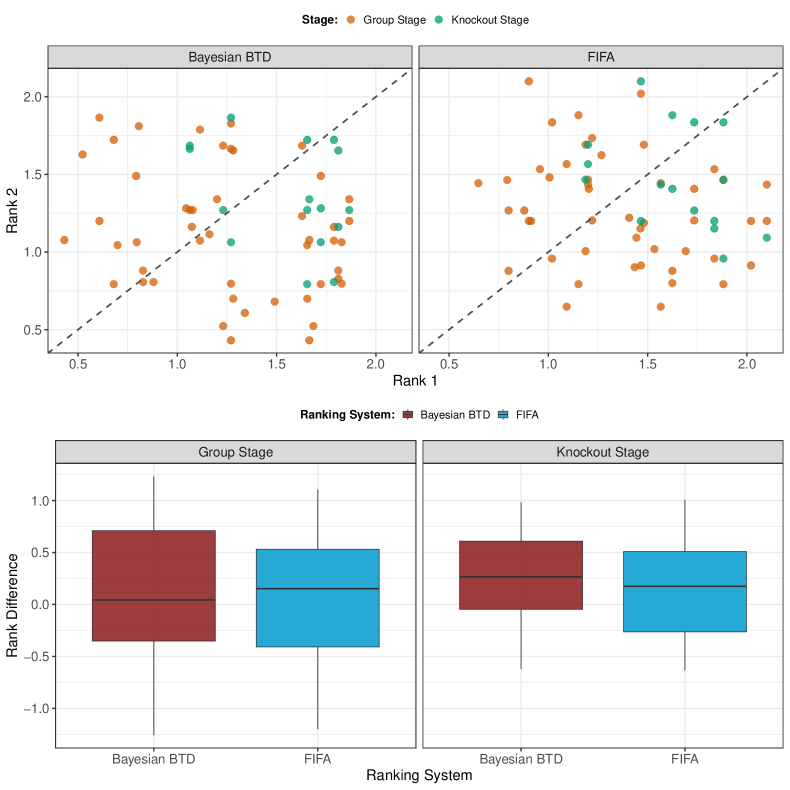
Figure 1: World Cup 2022: the top panel displays scatterplots comparing the ranks of teams in both the group stage (orange dots) and knockout stage (green dots) under the two ranking systems. The dashed grey line represents the bisector. The bottom panel presents boxplots of rank differences for the FIFA ranking (blue) and the Bayesian BTD derived ranking (red) across the two World Cup stages.

The main appeal of these models lies in their ability to predict the outcome of football matches. Figure 2 illustrates the predictive accuracy of dynamic Poisson models and machine learning algorithms, measured by the Brier Score, across both group and knockout stages. The goal-based statistical models perform slightly better than the result-based methods during the group stage. In contrast, the machine learning approaches show better predictive accuracy in the knockout stage, where results may be less predictable. A similar trend is seen with ranking systems. While the FIFA ranking system shows a marginally better predictive accuracy in the group stage, the Bayesian BTD ranking demonstrates overall better performance during the knockout stage. This suggests that the Bayesian BTD ranking is particularly apt at predicting outcomes when teams have comparable strength, which is often the case in the latter stages of the competition.

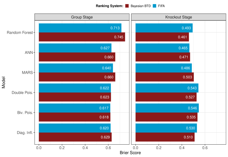
Figure 2: World Cup 2022: Brier score for the FIFA ranking (blue) and the Bayesian BTD derived ranking (red) across the two World Cup stages.

4.2 2024 Africa Cup of Nations

In this section, we fit the considered statistical models and machine learning algorithms to the data from the most recent Africa Cup of Nations (AFCON) tournament held in Ivory Coast. Notably, the AFCON competition differs from the FIFA World Cup in that the participating teams tend to be more similar in terms of overall strength even during the group stage, making it a compelling case for analyzing the effectiveness of the Bayesian BTD ranking system. In order to conduct this analysis, we use as training set the data from matches played throughout the period 2018 to the end of 2023. Furthermore, the Bayesian BTD model was executed within this same period to generate team rankings. In addition, the FIFA ranking employed correspond to those published on December 21st, available at https://inside.fifa.com/fifa-world-ranking/men?dateId=id14233.

In this scenario, the Bayesian BTD derived rankings exhibit less variability compared to the FIFA ranking, in both the group and knockout stages, as illustrated in the top panel of Figure 3. Furthermore, the boxplots displayed in the bottom panel of Figure 3 show a significant reduction in variance for both ranking systems as we move from the group stage to the knockout stage. However, contrary to what observed in the World Cup, the Bayesian BTD derived ranking exhibit lower variance compared to the FIFA ranking in the group stage. This may indicate that the Bayesian BTD ranking more accurately reflect the inherent similarity in team strengths within this tournament stage.

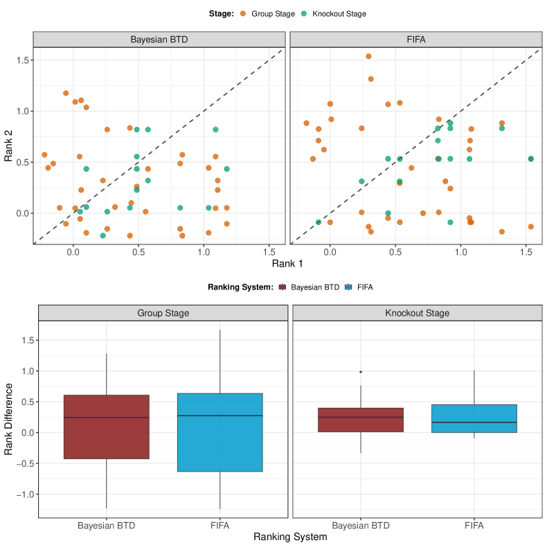
Figure 3: Africa Cup 2023: the top panel displays scatterplots comparing the ranks of teams in both the group stage (orange dots) and knockout stage (green dots) under the two ranking systems. The dashed grey line represents the bisector. The bottom panel presents boxplots of rank differences for the FIFA ranking (blue) and the Bayesian BTD derived ranking (red) across the two Africa Cup stages.

As reported in Figure 4, all the machine learning algorithms presents similar prediction performance in the group stage of the AFCON. However, random forests show the weakest performance in the knockout stage. Furthermore, the other machine learning algorithms and statistical models exhibited similar levels of predictive accuracy in both stages, with statistical models performing slightly better in the group stage. In particular, the inclusion of this alternative ranking system generally improved the predictive performance of most of the statistical models evaluated in the knockout stage.

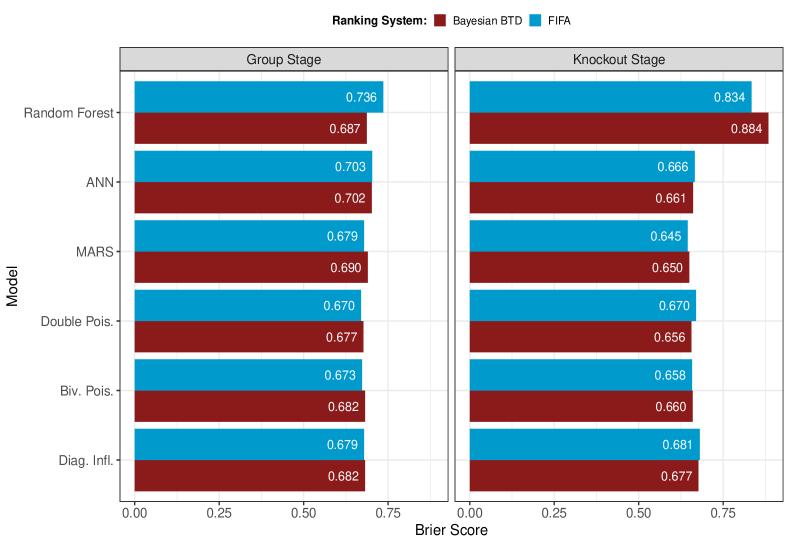
Figure 4: Africa Cup 2023: Brier score for the FIFA ranking (blue) and the Bayesian BTD derived ranking (red) across the two Africa Cup stages.

5 Discussion

This paper investigates the potential improvement in predictive performance of statistical goal-based methods and machine learning result-based algorithms when a ranking system is incorporated as an additional predictor variable. We analyze data from the recent 2022 FIFA World Cup in Qatar and the 2023 Africa Cup of Nations in Ivory Coast. Specifically, we explore the effectiveness of a Bayesian Bradley-Terry-Davidson derived ranking system in enhancing prediction accuracy compared to the well-established FIFA ranking system. We compare the performance of these two ranking systems across different tournament stages to identify their relative strengths and weaknesses in predicting match outcomes.

While both the FIFA ranking and the Bayesian BTD derived ranking provide valuable information for predicting outcomes, their effectiveness depends on the stage of the tournament. The FIFA ranking tends to be more accurate during the group stages of the 2022 World Cup, which features a more heterogeneous team strengths. Conversely, the Bayesian BTD derived ranking is particularly effective in the group stage of the 2023 AFCON, and it also presents slightly better predictive performances in the knockout stages of both the World Cup and the AFCON. These stages typically exhibit smaller differences in team strengths. Consequently, this result suggests that the Bayesian BTD model effectively captures shifts in team strengths, making it especially valuable in tournaments where competing team are similar, such as the AFCON, or in stages where the teams exhibit comparable strengths.

It is important to note that while the Bayesian BTD derived ranking is a valuable alternative, it is more computationally intensive compared to the standard FIFA ranking. Specifically, this approach involves a two-step procedure. First, the Bayesian BTD model needs to be computed to derive the ranking, and only then the derived ranking can be used as additional predictor in the models being considered.

However, the potential to enhance the accuracy and predictive performances of these models remains significant. Further development could involve refining the Bayesian BTD model to include additional variables that impact match outcomes. These could include the overall market value of the players involved in a specific team, the number of Champions League players, an indicator of the hosting country or of the teams in its neighbourhood. Even economic variables such as the GDP per capita or the national population size may be interesting. Furthermore, the implementation of a dynamic methodology, that enables the continuous adjustment for fluctuations in team strength over the course of a season or tournament, could potentially result in enhanced prediction accuracy.

The potential application of Bayesian Bradley-Terry derived rankings, as an alternative for the FIFA ranking or similar systems, represents a promising area for research. Further comparative studies across different sports or competition structures will be conducted to validate the effectiveness of the Bradley-Terry models. As broadly remarked, the interplay between the type of competition, the adopted ranking, and the chosen methodology represents an hot topic for football modellers and deserves a deep and further understanding, both in international matches and domestic leagues.

Software and Data Availability

All analyses were conducted in the R programming language version $4.2.3$ (R Core Team,, 2023). The code to reproduce this manuscript are openly available at https://github.com/RoMaD-96/Bayesian_BTD. The data are available on Kaggle at https://www.kaggle.com/datasets/martj42/international-football-results-from-1872-to-2017.

References

- Abreu et al., (2013) Abreu, P. H., Silva, D. C., Mendes-Moreira, J., Reis, L. P., and Garganta, J. (2013). Using multivariate adaptive regression splines in the construction of simulated soccer team’s behavior models. International Journal of Computational Intelligence Systems, 6:893–910.
- Baio and Blangiardo, (2010) Baio, G. and Blangiardo, M. (2010). Bayesian hierarchical model for the prediction of football results. Journal of Applied Statistics, 37(2):253–264.
- Beaver and Gokhale, (1975) Beaver, R. J. and Gokhale, D. V. (1975). A model to incorporat within-pair order effects in paired comparisons. Communications in Statistics, 4(10):923–939.
- Bradley and Terry, (1952) Bradley, R. A. and Terry, M. E. (1952). Rank analysis of incomplete block designs: I. the method of paired comparisons. Biometrika, 39(3/4):324–345.
- Breiman, (2001) Breiman, L. (2001). Random forests. Machine Learning, 45(1):5–32.
- Brier, (1950) Brier, G. W. (1950). Verification of forecasts expressed in terms of probability. Monthey Weather Review,, 78(1):1–3.
- Caron and Doucet, (2012) Caron, F. and Doucet, A. (2012). Efficient Bayesian inference for generalized Bradley–Terry models. Journal of Computational and Graphical Statistics, 21(1):174–196.
- Carpita et al., (2019) Carpita, M., Ciavolino, E., and Pasca, P. (2019). Exploring and modelling team performances of the Kaggle European soccer database. Statistical Modelling, 19(1):74–101.
- Cattelan, (2012) Cattelan, M. (2012). Models for paired comparison data: A review with emphasis on dependent data. Statistical Science, 27(3):412 – 433.
- Cattelan et al., (2012) Cattelan, M., Varin, C., and Firth, D. (2012). Dynamic Bradley–Terry modelling of sports tournaments. Journal of the Royal Statistical Society Series C: Applied Statistics, 62(1):135–150.
- Chen and Smith, (1984) Chen, C. and Smith, T. M. (1984). A Bayes-type estimator for the Bradley-Terry model for paired comparison. Journal of Statistical Planning and Inference, 10(1):9–14.
- Danisik et al., (2018) Danisik, N., Lacko, P., and Farkas, M. (2018). Football match prediction using players attributes. pages 201–206.
- Davidson, (1970) Davidson, R. R. (1970). On extending the Bradley-Terry model to accommodate ties in paired comparison experiments. Journal of the American Statistical Association, 65(329):317–328.
- Davidson and Beaver, (1977) Davidson, R. R. and Beaver, R. J. (1977). On extending the Bradley-Terry model to incorporate within-pair order effects. Biometrics, 33(4):693–702.
- Davidson and Solomon, (1973) Davidson, R. R. and Solomon, D. L. (1973). A Bayesian approach to paired comparison experimentation. Biometrika, 60(3):477–487.
- Dixon and Coles, (1997) Dixon, M. J. and Coles, S. G. (1997). Modelling association football scores and inefficiencies in the football betting market. Journal of the Royal Statistical Society: Series C (Applied Statistics), 46(2):265–280.
- Egidi and Palaskas., (2022) Egidi, L. and Palaskas., V. (2022). footBayes: Fitting Bayesian and MLE Football Models. R package version 0.2.0.
- Egidi et al., (2018) Egidi, L., Pauli, F., and Torelli, N. (2018). Combining historical data and bookmakers’ odds in modelling football scores. Statistical Modelling, 18(5-6):436–459.
- Egidi and Torelli, (2021) Egidi, L. and Torelli, N. (2021). Comparing goal-based and result-based approaches in modelling football outcomes. Social Indicators Research, 156.
- Fahrmeir and Tutz, (1994) Fahrmeir, L. and Tutz, G. (1994). Dynamic stochastic models for time-dependent ordered paired comparison systems. Journal of the American Statistical Association, 89(428):1438–1449.
- Ford, (1957) Ford, L. R. (1957). Solution of a ranking problem from binary comparisons. American Mathematical Monthly, 64:28–33.
- Friedman, (1991) Friedman, J. H. (1991). Multivariate adaptive regression splines. The Annals of Statistics, 19(1):1 – 67.
- Glickman, (1999) Glickman, M. E. (1999). Parameter estimation in large dynamic paired comparison experiments. Journal of the Royal Statistical Society. Series C (Applied Statistics), 48(3):377–394.
- Glickman, (2001) Glickman, M. E. (2001). Dynamic paired comparison models with stochastic variances. Journal of Applied Statistics, 28(6):673–689.
- Groll and Abedieh, (2013) Groll, A. and Abedieh, J. (2013). Spain retains its title and sets a new record – generalized linear mixed models on European football championships. Journal of Quantitative Analysis in Sports, 9(1):51–66.
- Groll et al., (2019) Groll, A., Cristophe, L., Hans, V. E., and Gunther, S. (2019). A hybrid random forest to predict soccer matches in international tournaments. Journal of Quantitative Analysis in Sports, 15(4):271–287.
- Groll et al., (2021) Groll, A., Hvattum, L. M., Ley, C., Popp, F., Schauberger, G., Van Eetvelde, H., and Zeileis, A. (2021). Hybrid machine learning forecasts for the UEFA EURO 2020. arXiv preprint arXiv:2106.05799.
- Huang and Chang, (2010) Huang, K.-Y. and Chang, W.-L. (2010). Neural network method for prediction of 2006 World Cup football game. In The 2010 International Joint Conference on Neural Networks (IJCNN), pages 1–8.
- Hucaljuk and Rakipovic, (2011) Hucaljuk, J. and Rakipovic, A. (2011). Predicting football scores using machine learning techniques. 2011 Proceedings of the 34th International Convention MIPRO, pages 1623–1627.
- Hunter, (2004) Hunter, D. R. (2004). MM algorithms for generalized Bradley-Terry models. The Annals of Statistics, 32(1):384–406.
- Issa Mattos and Martins Silva Ramos, (2020) Issa Mattos, D. and Martins Silva Ramos, E. (2020). bpc: A package for Bayesian paired comparison analysis.
- Issa Mattos and Martins Silva Ramos, (2022) Issa Mattos, D. and Martins Silva Ramos, É. (2022). Bayesian paired comparison with the bpcs package. Behavior Research Methods, 54(4):2025–2045.
- Karlis and Ntzoufras, (2003) Karlis, D. and Ntzoufras, I. (2003). Analysis of sports data by using bivariate Poisson models. Journal of the Royal Statistical Society: Series D (The Statistician), 52(3):381–393.
- Karlis and Ntzoufras, (2009) Karlis, D. and Ntzoufras, I. (2009). Bayesian modelling of football outcomes: using the Skellam’s distribution for the goal difference. IMA Journal of Management Mathematics, 20(2):133–145.
- Koning, (2000) Koning, R. H. (2000). Balance in competition in Dutch soccer. Journal of the Royal Statistical Society: Series D (The Statistician), 49(3):419–431.
- Koopman and Lit, (2015) Koopman, S. J. and Lit, R. (2015). A dynamic bivariate Poisson model for analysing and forecasting match results in the English Premier League. Journal of the Royal Statistical Society. Series A (Statistics in Society), 178(1):167–186.
- Kuhn, (2022) Kuhn, M. (2022). Caret: Classification and regression training. R package version 6.0-93.
- Leonard, (1977) Leonard, T. (1977). An alternative Bayesian approach to the Bradley-Terry model for paired comparisons. Biometrics, 33(1):121–132.
- Luce, (1959) Luce, R. (1959). Individual choice behavior: A theoretical analysis. Wiley.
- Maher, (1982) Maher, M. J. (1982). Modelling association football scores. Statistica Neerlandica, 36(3):109–118.
- Ntzoufras, (2011) Ntzoufras, I. (2011). Bayesian Modeling Using WinBUGS, volume 698. John Wiley & Sons, Hoboken, New Jersey, USA.
- Osei and Davidov, (2022) Osei, P. P. and Davidov, O. (2022). Bayesian linear models for cardinal paired comparison data. Computational Statistics & Data Analysis, 172:107481.
- Owen, (2011) Owen, A. (2011). Dynamic Bayesian forecasting models of football match outcomes with estimation of the evolution variance parameter. IMA Journal of Management Mathematics, 22(2):99–113.
- R Core Team, (2023) R Core Team (2023). R: A Language and Environment for Statistical Computing. R Foundation for Statistical Computing, Vienna, Austria.
- Rao and Kupper, (1967) Rao, P. V. and Kupper, L. L. (1967). Ties in paired-comparison experiments: A generalization of the Bradley-Terry model. Journal of the American Statistical Association, 62(317):194–204.
- Rue and Øyvind Salvesen, (2000) Rue, H. and Øyvind Salvesen (2000). Prediction and retrospective analysis of soccer matches in a league. Journal of the Royal Statistical Society. Series D (The Statistician), 49(3):399–418.
- Schauberger and Groll, (2018) Schauberger, G. and Groll, A. (2018). Predicting matches in international football tournaments with random forests. Statistical Modelling, 18(5-6):460–482.
- Spiegelhalter and Ng, (2009) Spiegelhalter, D. and Ng, Y.-L. (2009). One match to go! Significance, 6(4):151–153.
- Springall, (1973) Springall, A. (1973). Response surface fitting using a generalization of the Bradley-Terry paired comparison model. Journal of the Royal Statistical Society Series C: Applied Statistics, 22(1):59–68.
- Szczecinski and Roatis, (2022) Szczecinski, L. and Roatis, I.-I. (2022). FIFA ranking: Evaluation and path forward. Journal of Sports Analytics, 8(4):231–250.
- Tian et al., (2023) Tian, X.-Y., Shi, J., Shen, X., and Song, K. (2023). A spectral approach for the dynamic Bradley-Terry model. arXiv preprint arXiv:2307.16642.
- Wainer, (2023) Wainer, J. (2023). A Bayesian Bradley-Terry model to compare multiple ml algorithms on multiple data sets. Journal of Machine Learning Research, 24(341):1–34.
- Whelan, (2017) Whelan, J. T. (2017). Prior distributions for the bradley-terry model of paired comparisons. arXiv preprint arXiv:1712.05311.