Rounding Large Independent Sets on Expanders

Abstract

We develop a new approach for approximating large independent sets when the input graph is a one-sided spectral expander — that is, the uniform random walk matrix of the graph has the second eigenvalue bounded away from 1. Consequently, we obtain a polynomial time algorithm to find linear-sized independent sets in one-sided expanders that are almost $3$-colorable or are promised to contain an independent set of size $(1/2-\varepsilon)n$. Our second result above can be refined to require only a weaker vertex expansion property with an efficient certificate. Somewhat surprisingly, we observe that the analogous task of finding a linear-sized independent set in almost $4$-colorable one-sided expanders (even when the second eigenvalue is $o_{n}(1)$) is NP-hard, assuming the Unique Games Conjecture.

All prior algorithms that beat the worst-case guarantees for this problem rely on bottom eigenspace enumeration techniques (following the classical spectral methods of Alon and Kahale [AK97]) and require two-sided expansion, meaning a bounded number of negative eigenvalues of magnitude $\Omega(1)$. Such techniques naturally extend to almost $k$-colorable graphs for any constant $k$, in contrast to analogous guarantees on one-sided expanders, which are Unique Games-hard to achieve for $k\geqslant 4$.

Our rounding builds on the method of simulating multiple samples from a pseudodistribution introduced in [BBK⁺21] for rounding Unique Games instances. The key to our analysis is a new clustering property of large independent sets in expanding graphs — every large independent set has a larger-than-expected intersection with some member of a small list — and its formalization in the low-degree sum-of-squares proof system.

1 Introduction

Finding large independent sets is a notoriously hard problem in the worst case. The best-known algorithms can only find independent sets of size $\widetilde{O}(\log^{2}n)$ in $n$-vertex graphs with independent sets of near-linear size [Fei04]. In this paper, we are interested in the important setting when the input graph contains an independent set of size $cn$ for a large constant $c<1/2$. When $c=1/2-\varepsilon$ for tiny enough $\varepsilon>0$, a generalization of an algorithm by Karger, Motwani, and Sudan [KMS98] finds an independent set of size $n^{1-O(\varepsilon)}$ (see Appendix B). When $c\ll 1/2$, all known efficient algorithms [BH92, AK98] can only find independent sets of size $n^{\delta(c)}$ for some $\delta(c)<1$, and this is true even when the graph is $k$-colorable (thus $c\geqslant 1/k$), with only small constant improvements on the exponent following a long line of works [Wig83, Blu94, BK97, KMS98, ACC06, Chl09, KT17]. To summarize, in the worst-case, even when $c$ approaches $1/2$, our best-known efficient algorithms can only find independent sets of size a polynomial factor smaller than $n$.

There is evidence that the difficulties in improving the above algorithms might be inherent. Assuming the Unique Games Conjecture (UGC), for any constant $\varepsilon>0$, it is NP-hard to find an independent set of size $\varepsilon n$ even when the input graph contains an independent set of size $(1/2-\varepsilon)n$ [KR08, BK09]. Similar hardness results persist in the related setting of $3$-colorable graphs [DS05, DMR06, DKPS10, KS12].

Given the above worst-case picture, a substantial effort over the past three decades has explored algorithms that work under natural structural assumptions on the input graphs. One line of work studies planted average-case models for independent set [Kar72, Jer92, Kuč95] and coloring [BS95, AK97], as well as their semirandom generalizations [BS95, FK01, CSV17, MMT20, BKS23] with myriad connections to other areas [BR13, HWX15, BBH18, KM18]. A related body of research has focused on graphs that satisfy natural, deterministic assumptions, such as expansion, which isolate simple and concrete properties of random instances that enable efficient algorithms. This approach has been explored for Unique Games [Tre08, AKK⁺08, MM11, ABS15, BBK⁺21] and related problems such as Max-Cut and Sparsest Cut [DHV16, RV17], and has been instrumental in making progress even for worst-case instances, for e.g., leading eventually to a subexponential algorithm for arbitrary UG instances [ABS10]. Over the past decade, such assumptions have also been investigated for independent set and coloring [AG11, DF16, KLT18]. In particular, a recent work of David and Feige [DF16] gave polynomial-time algorithms for finding large independent sets in planted $k$-colorable expander graphs.

Prior Works and One-Sided vs Two-Sided Expansion.

There is a crucial difference between the expansion assumptions in prior works on coloring vs other problems, which we now discuss. A $d$-regular graph whose normalized adjacency matrix $\frac{1}{d}A$ (a.k.a., the uniform random walk matrix) has eigenvalues $1=\lambda_{1}\geqslant\lambda_{2}\geqslant\cdots\geqslant\lambda_{n}$ is called a one-sided spectral expander if $\lambda_{2}\leqslant\lambda$, and a two-sided spectral expander if $\max\{\lambda_{2},|\lambda_{n}|\}\leqslant\lambda$ for some $\lambda<1$ (here $1-\lambda_{2}$ is termed the spectral gap). Most known algorithms for problems (e.g., Unique Games and other constraint satisfaction problems) on expanders only need one-sided spectral expansion, as they primarily rely on the edge expansion of the graph, a combinatorial property closely related to $\lambda_{2}$ via Cheeger’s inequality. In contrast, algorithms for finding independent sets in expanders with a planted $k$-coloring rely on two-sided spectral expansion (i.e., control of even the negative end of the spectrum).

This is not just a technical quirk; the foundational observation underlying such algorithms (due to Alon and Kahale [AK97], following Hoffman [Hof70]) is that a random graph is a two-sided spectral expander (thus, has no large negative eigenvalues) and that planting a $k$-coloring in it introduces negative eigenvalues of large magnitude, whose corresponding eigenvectors are correlated with indicator vectors of the color classes. This allows using the bottom eigenvectors of the graph to obtain a coarse spectral clustering. All the works above, including those on deterministic expander graphs [DF16], build on this basic observation for their algorithmic guarantees.

This basic idea becomes inapplicable if we are working with one-sided spectral expanders that behave markedly differently in the context of graph coloring. To illustrate this point, we observe the following proposition with a simple proof (see Appendix A) which implies that there is likely no efficient algorithm to find any $\Omega(n)$-sized independent set in an $\varepsilon$-almost $4$-colorable graph (i.e., $4$-colorable if one removes $\varepsilon$ fraction of vertices), even when promised to have nearly perfect one-sided spectral expansion with $\lambda_{2}\leqslant o_{n}(1)$!

Proposition 1.1 (See Proposition A.2).

Assuming the Unique Games Conjecture, for any constants $\varepsilon,\gamma>0$, it is NP-hard to find an independent set of size $\gamma n$ in an $n$-vertex regular graph which is $\varepsilon$-almost $4$-colorable and has $\lambda_{2}\leqslant o_{n}(1)$.

This is in sharp contrast to David and Feige’s algorithm [DF16] which shows how to find a planted $k$-coloring in a sufficiently strong two-sided spectral expander for any constant $k$.

We prove Proposition 1.1 by a reduction from the UG-hardness of finding linear-sized independent sets in $\varepsilon$-almost $2$-colorable graphs [BK09] and guaranteeing one-sided expansion in addition at the cost of obtaining an almost $4$-colorable graph. A similar reduction allows us to show hardness of finding linear-sized independent sets in exactly $6$-colorable ($\varepsilon=0$) one-sided spectral expanders (see Proposition A.6). We remark that the instances produced by the reduction must necessarily have many negative eigenvalues, otherwise spectral clustering algorithms based on the bottom eigenspace [AK97, DF16] can likely find linear-sized independent sets.

This Work.

We are thus led to the main question studied in this work:

Can polynomial-time algorithms find a large independent set in a $3$-colorable one-sided spectral expander?

Proposition 1.1 injects a fair amount of intrigue into this question, but our motivations for studying it go farther: an affirmative answer would necessarily require developing a new algorithmic approach that departs from spectral clustering based on bottom eigenvectors.

Let us spoil the intrigue: in this work, we develop new algorithms for finding large independent sets via rounding sum-of-squares (SoS) relaxations. Our polynomial-time algorithms succeed in finding linear-sized independent sets in almost $3$-colorable graphs that satisfy one-sided spectral expansion. Given the UG-hardness (i.e., Proposition 1.1) of finding linear-sized independent sets in an almost $4$-colorable one-sided expander, we obtain a stark and surprising difference between almost $3$-colorable and almost $4$-colorable one-sided expander graphs.

Theorem 1.

There is a polynomial-time algorithm that, given an $n$-vertex regular $10^{-4}$-almost $3$-colorable one-sided spectral expander with $\lambda_{2}\leqslant 10^{-4}$, outputs an independent set of size at least $10^{-4}n$.

We note that we cannot, in general, hope to find a coloring of the graph by iterating on the graph obtained by removing the vertices in an independent set, as the remaining graph may not be an expander. This difficulty appears to be inherent even when the graph has two-sided expansion. Towards a formal barrier, David and Feige [DF16] proved that it is NP-hard to find a $3$-coloring planted in a random host graph with not-too-large degree (even though they show an algorithm for finding a partial $3$-coloring in such a graph).

Our techniques succeed without the $3$-colorability assumption if the input graph has an independent set of size $(1/2-\varepsilon)n$, and satisfies a weaker quantitative one-sided spectral expansion.

Theorem 2.

For every positive $\varepsilon\leqslant 0.001$, there is a polynomial-time algorithm that, given an $n$-vertex regular graph that contains an independent set of size $(\frac{1}{2}-\varepsilon)n$ and is a one-sided spectral expander with $\lambda_{2}\leqslant 1-40\varepsilon$, outputs an independent set of size at least $10^{-3}n$.

Note that we get an algorithm for $\varepsilon$-almost $2$-colorable one-sided expanders as an immediate corollary. Before this work, no algorithm that beat the worst-case guarantee of outputting a $n^{1-O(\varepsilon)}$-sized independent set was known in this setting.

With more work, our algorithms succeed even under the weaker notion of vertex (as opposed to spectral) expansion defined below.

Definition 1.2 (Small-set vertex expansion).

The small-set vertex expansion (SSVE) of a graph $G=(V,E)$, with size parameter $\delta\in(0,1/2]$, is defined as

$$\Psi_{\delta}(G)\coloneqq\min_{S\subseteq V:0<|S|\leqslant\delta|V|}\frac{|N_{G}(S)|}{|S|}\,,$$

where $N_{G}(S)$ is the set of neighbors of $S$: $N_{G}(S)=\{u\notin S:\exists v\in S,\ \{u,v\}\in E\}$. We say that $G$ is a $\delta$-SSVE if $\Psi_{\delta}(G)\geqslant 2$.

This is a strictly weaker notion than edge expansion since a graph can be a vertex expander without being an edge expander. Our algorithm succeeds on graphs that admit efficient certificates of vertex expansion (see Definition 6.3; we only need certificates for expansion of small sets). Unlike edge expansion, which naturally comes with a spectral certificate, such efficient certificates are unfortunately not currently known. However, as a proof of concept, we show in Section 8 that the noisy hypercube, despite not being a spectral expander, admits a non-trivially small degree sum-of-squares certificate of SSVE.

Theorem 3 (Informal Theorem 6.1).

For all $\delta\in(0,1/2)$, suppose $G$ is an $n$-vertex graph that admits a low-degree sum-of-squares certificate of $\delta$-small-set vertex expansion (SSVE) and has an independent set of size $(\frac{1}{2}-\operatorname{poly}(\delta))n$, then there is an algorithm that runs in time $n^{\operatorname{poly}(1/\delta)}$ and outputs an independent set of size $\operatorname{poly}(\delta)n$.

As an immediate corollary of Theorem 3 (see Corollary 8.4), we get a sub-exponential-size certificate that the noisy hypercube does not have large independent sets; see Section 8 for details and discussions.

Our Techniques.

The key conceptual idea underlying our algorithms is establishing a clustering property of independent sets in expanding graphs, reminiscent of the cluster structure [ART06, GS17] in the solution space geometry in random optimization problems, which may be interesting on its own. Specifically, we prove that every large independent set in an expander must be “better-than-random” correlated with a member of any small list of large independent sets — that is, the intersection is $\delta n$ larger than the expected intersection between random sets of similar size for some absolute constant $\delta>0$. Our algorithms are based on a new rounding scheme for constant-degree sum-of-squares relaxations that work whenever such an (apparently mild) correlation can be established along with a low-degree sum-of-squares formalization of it. Our rounding scheme is based on the idea of simulating multiple independent samples from the underlying pseudodistribution, a technique introduced in [BBK⁺21] for Unique Games and strengthened further in [BM23]. We discuss our technical ideas in more detail in the next section.

2 Technical Overview

This section provides a brief overview of our rounding framework and analysis. In Section 2.1, we briefly discuss the clustering property and how it leads to our rounding algorithm for one-sided spectral expanders. The rounding for independent sets on certified small-set vertex expanders, though based on similar principles, is more involved and we discuss it briefly in Section 2.2. Then, we describe the proof of the clustering property of independent sets in Section 2.3 and the clustering property of $3$-colorings in Section 2.4. The rounding for 3-colorable graphs follows a similar rounding framework, and we refer the reader to Section 5 for details.

Polynomial Formulation and SoS Relaxation.

All solutions to the following polynomial system are independent sets of size $\geqslant(1/2-\varepsilon)n$.

$$\frac{1}{n}\sum_{u\in V} x_{u}\geqslant\frac{1}{2}-\varepsilon,$$ (1)

$$x_{u}^{2}=x_{u}\,, \forall u\in V\,,$$

$$x_{u}x_{v}=0\,, \forall\{u,v\}\in E.$$

Our algorithm involves solving a constant-degree sum-of-squares relaxation of this system and rounding the resulting solution, a.k.a., a pseudodistribution (see Section 3.1 for background). For a reader unfamiliar with the sum-of-squares method for algorithm design, it is helpful to think of $\mu$ as constant-degree moments (i.e., expectations under $\mu$ of any constant-degree polynomial of $x$) of a probability distribution over $x\in\{0,1\}^{n}$ indicating independent sets of size $\geqslant(\frac{1}{2}-\varepsilon)n$.

2.1 Rounding on One-Sided Spectral Expanders

Let $G$ be any regular one-sided spectral expander with $\lambda_{2}(G)\leqslant 1-O(\varepsilon)$ containing an independent set of size $(1/2-\varepsilon)n$. Our approach can be summarized in two steps:

1. We show (in Lemma 2.1) that there are essentially two $(1/2-\varepsilon)n$-sized independent sets in $G$ — given any three independent sets $x^{(1)},x^{(2)},x^{(3)}$, two of them have a non-trivially large intersection, $\mathbb{E}_{u}[x^{(i)}x^{(j)}]>1/2-\nu$ for some $\nu\approx 0$ and $i\neq j\in[3]$.

2. Given any three $(1/2-\varepsilon)n$-sized independent sets, ${\bm{x}}:=(x^{(1)},x^{(2)},x^{(3)})$, we define $\Phi({\bm{x}}):=\mathbb{E}_{u}[x_{u}^{(1)}x_{u}^{(2)}]^{2}+\mathbb{E}_{u}[x_{u}^{(2)}x_{u}^{(3)}]^{2}+\mathbb{E}_{u}[x_{u}^{(1)}x_{u}^{(3)}]^{2}$ which is $\geqslant 1/4-\nu^{\prime}$ as a consequence of (1). Here, $\mathbb{E}_{u}$ is the average with respect to a uniformly random $u\in[n]$ and thus $\Phi({\bm{x}})$ measures the average pairwise intersection between $x^{(1)},x^{(2)},x^{(3)}$.

3. The above implies that $\Phi({\bm{x}})$ is large in expectation over $x^{(1)},x^{(2)},x^{(3)}$ drawn independently from $\mu$, i.e., $\Phi(\mu):=\widetilde{\mathbb{E}}_{{\bm{x}}\sim\mu^{\otimes 3}}[\Phi({\bm{x}})]\geqslant 1/4-\nu^{\prime}$. In this case, we show how to apply a simple rounding algorithm on $\mu$ to obtain a large independent set in $G$.

In fact, by defining a variant of $\Phi$, our rounding analysis works as long as the intersection in (1) is non-trivially larger than expected, i.e., intersection $\geqslant(1/4+\delta)n$, where $n/4$ is the expected intersection between random sets of size $\approx n/2$. However, the analysis is simpler in the case where the intersection is $\geqslant 1/2-\nu$.

We also note that the strategy of drawing multiple samples from a pseudodistribution to round high-degree SoS relaxations was first introduced in [BBK⁺21]. In their application for rounding Unique Games on certified small-set expanders, they considered a certain “shift-partition potential” (which measured the correlation between two solutions for the input UG instance) instead of the function $\Phi(\mu)$ above.

We will discuss how (1) above is proved in Section 2.3. In the rest of the section, we discuss how we round given that $\Phi(\mu)$ is large.

Rounding when $\Phi(\mu)$ is large.

In order to understand the intuition behind our rounding, notice that for 3 random subsets of $[n]$ of size $(1/2-\varepsilon)n$, the pairwise agreement function $\Phi$ would be $\approx 3\cdot(1/4)^{2}=3/16$. Thus, if $\Phi(\mu)\geqslant 1/4-\nu^{\prime}>3/16$ for some small $\nu^{\prime}$, then three draws from $\mu$ must be non-trivially correlated – signalling that the distribution is supported over two “distinct” independent sets. In this case, one would expect to condition $\mu$ so that the resulting distribution $\mu^{\prime}$ is essentially supported on a unique assignment, in the sense that two independent draws from $\mu^{\prime}$ have intersection $\geqslant 1/4+\delta$. Once we have this, we can show a simple rounding algorithm on $\mu^{\prime}$ outputs an $\Omega(\delta n)$-sized independent set. Let us formalize this intuition. We have that,

$$\widetilde{\mathbb{E}}_{{\bm{x}}\sim\mu^{\otimes 3}}[\Phi({\bm{x}})]=3\cdot\widetilde{\mathbb{E}}_{x^{(1)},x^{(2)}\sim\mu}\left[\mathbb{E}_{u}[x_{u}^{(1)}x_{u}^{(2)}]^{2}\right]\geqslant 1/4-O(\varepsilon)\,,$$

implying that $\widetilde{\mathbb{E}}_{x^{(1)},x^{(2)}}[\mathbb{E}_{u}[x_{u}^{(1)}x_{u}^{(2)}]^{2}]\geqslant 1/12-O(\varepsilon)>1/16+\delta$ for a constant $\delta>0$ if $\varepsilon$ is a small enough constant. Simplifying further using the independence of $x^{(1)}$ and $x^{(2)}$ we get,

$$\widetilde{\mathbb{E}}_{x^{(1)},x^{(2)}\sim\mu}\left[\mathbb{E}_{u}[x_{u}^{(1)}x_{u}^{(2)}]^{2}\right]=\widetilde{\mathbb{E}}\left[\mathbb{E}_{u,v}[x_{u}^{(1)}x_{v}^{(1)}x_{u}^{(2)}x_{v}^{(2)}]\right]=\mathbb{E}_{u,v}\left[\widetilde{\mathbb{E}}[x_{u}x_{v}]^{2}\right]>1/16+\delta\,.$$

We apply a certain repeated conditioning procedure (that reduces “global correlation” [BRS11, RT12]) to obtain a modified pseudodistribution $\mu^{\prime}$ that satisfies all the original constraints and, in addition, satisfies that for most pairs of vertices $u,v\in[n]$: $\widetilde{\mathbb{E}}_{\mu^{\prime}}[x_{u}x_{v}]\approx\widetilde{\mathbb{E}}_{\mu^{\prime}}[x_{u}]\widetilde{\mathbb{E}}_{\mu^{\prime}}[x_{v}]$ (where the approximation hides additive constant errors). Thus, we have

$$\mathbb{E}_{u,v}\left[\widetilde{\mathbb{E}}_{\mu^{\prime}}[x_{u}x_{v}]^{2}\right]\approx\mathbb{E}_{u,v}\left[\widetilde{\mathbb{E}}_{\mu^{\prime}}[x_{u}]^{2}\widetilde{\mathbb{E}}_{\mu^{\prime}}[x_{v}]^{2}\right]=\mathbb{E}_{u}\big{[}\widetilde{\mathbb{E}}_{\mu^{\prime}}[x_{u}]^{2}\big{]}^{2}>1/16+\delta\,.$$

This means that two independent samples from $\mu^{\prime}$ have larger intersection than random: $\widetilde{\mathbb{E}}_{x^{(1)},x^{(2)}\sim\mu^{\prime}}[\mathbb{E}_{u}[x^{(1)}_{u}x^{(2)}_{u}]]=\mathbb{E}_{u}[\widetilde{\mathbb{E}}_{\mu^{\prime}}[x_{u}]^{2}]>1/4+\Omega(\delta)$. An averaging argument now yields that $\widetilde{\mathbb{E}}_{\mu}[x_{u}]>\frac{1}{2}$ for at least an $\Omega(\delta)$ fraction of the vertices. It is easy to check that this set of vertices is an independent set (see Fact 3.8) of size $\Omega(\delta n)$.

2.2 Rounding Independent Set on Small-Set Vertex Expanders

Our rounding and analysis follows a framework similar to the one presented for independent sets on one-sided spectral expanders, albeit each step itself being more technically involved.

1. If $G$ is a $\delta$-SSVE, then we show that there are at most $t=O(\log(1/\delta))$ essentially distinct $(1/2-\varepsilon)n$-sized independent sets. The exact notion of distinctness turns out to be more complicated (see Lemma 6.9 for the formal statement), but for this overview, we will work with a generalization of the statement we describe in the previous section: given any set of $2t$ independent sets ${\bm{x}}=(x^{(1)},\ldots,x^{(2t)})$ on $G$, there exist $t$ of them with intersection $\mathbb{E}_{u}[x_{u}^{(i_{1})}\ldots x_{u}^{(i_{t})}]>\delta$.

2. If $G$ is a certified-SSVE (Definition 6.3), in the sense that there is a degree-$D$ certificate that $\Psi_{\delta}(G)\geqslant 2$, then the above fact, formalized appropriately as a polynomial inequality, has a degree $O(tD)$ sum-of-squares proof.

3. We show how to round to a $\operatorname{poly}(\delta)n$-sized independent set given the SoS-version of the structural statement above.

Rounding under (2):

Suppose we have a pseudodistribution $\mu$ over independent sets of $G$, intuitively we should expect to condition on an event of probability $\geqslant\frac{1}{\binom{2t}{t}}$ to get $\mathcal{D}$ with the property that: $\widetilde{\mathbb{E}}_{\mathcal{D}^{\otimes t}}[\mathbb{E}_{u}[x_{u}^{(1)}\ldots x_{u}^{(t)}]]\geqslant\delta$. Once we have this, we can apply a simple argument to obtain an independent set of size $\Omega(\delta n)$. Formalizing this appropriately we can show that,

$$\widetilde{\mathbb{E}}_{\mu^{\otimes t}}\left[q({\bm{x}})\left\lparen\mathbb{E}_{u}\left[\prod_{i\in S}x_{u}^{(i)}\right]-\delta\right\rparen\right]>0,$$

for some $S\subseteq[2t]$ and SoS polynomial $q({\bm{x}})$. A natural strategy henceforth would be to condition/reweight $\mu^{\otimes t}$ on $q({\bm{x}})$ to get that $\widetilde{\mathbb{E}}_{\mu^{\otimes t}|q({\bm{x}})}[\mathbb{E}_{u}[x_{u}^{(1)}\ldots x_{u}^{(t)}]]\geqslant\delta$. This is what we were aiming for, except that there is a new issue — $\mu^{\otimes t}|q({\bm{x}})$ is no longer a product distribution, hence the natural rounding analysis breaks. To remedy this, we use tools from [BM23] to show that one can indeed condition on $q({\bm{x}})$, after performing a suitable preprocessing step, to get an approximately-product distribution which is then easy to round to a large independent set.

2.3 Intersection between Independent Sets on One-Sided Spectral Expanders

Let us now return to the combinatorial guts of our approach and discuss a proof of:

Lemma 2.1.

Let $G$ be a regular graph containing an independent set of size $(\frac{1}{2}-\varepsilon)n$ and has $\lambda_{2}(G)\leqslant 1-C\varepsilon$ for any small enough $\varepsilon$ and some large enough constant $C>0$. Then, for any $3$ independent sets of size at least $(\frac{1}{2}-\varepsilon)n$, two of them have an intersection of size $\geqslant(\frac{1}{2}-O(\frac{1}{C})-\varepsilon)n$.

Intersection between $2$ independent sets.

Let us start by understanding how the intersection between $2$ independent sets $I_{1},I_{2}$ (indicated by $x,y\in\{0,1\}^{n}$) in $G$ behaves. By assigning every vertex $u$ of $G$ the label $(x_{u},y_{u})$, we obtain a partition of vertices of $G$ based on the labels in $\{00,01,10,11\}$. We can now consider a graph on $4$ vertices (corresponding to the labels) and add an edge between two such labels (including self loops) if there is an edge between two vertices of the corresponding labels in $G$ (see Figure 1).

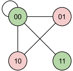
Figure 1: The gadget for $2$ independent sets.

Note that there are no edges between $01,10$ and $11$ because $x,y$ indicate independent sets. There can, however, be edges between vertices in the set $00$, hence the self-loop. Observe that the graph in Figure 1 is the tensor product $H\otimes H$ where $H$ is the $2$-vertex graph with vertex set $\{0,1\}$ and edges $(0,0)$ and $(0,1)$.

Let $\mathsf{wt}(ij)$ denote the fraction of vertices $u$ such that $x_{u}=i$ and $y_{u}=j$. The intersection between $I_{1},I_{2}$ is thus $\mathsf{wt}(11)$. We now observe the following fact about the sizes of $00$ and $11$:

Claim 2.2.

$\mathsf{wt}(00)\leqslant\mathsf{wt}(11)+2\varepsilon$.

Proof.

By the assumption that both $I_{1}$ and $I_{2}$ have size at least $(\frac{1}{2}-\varepsilon)n$, we have $\mathsf{wt}(11)+\mathsf{wt}(10)$ and $\mathsf{wt}(11)+\mathsf{wt}(01)\geqslant\frac{1}{2}-\varepsilon$, which means that $\mathsf{wt}(01)+\mathsf{wt}(10)+2\mathsf{wt}(11)\geqslant 1-2\varepsilon$. The proof follows by noting that $\mathsf{wt}(00)+\mathsf{wt}(01)+\mathsf{wt}(10)+\mathsf{wt}(11)=1$. ∎

We now use the expansion of $G$ to observe the following:

Claim 2.3.

Fix $\varepsilon>0$ small enough. If $\lambda_{2}\leqslant 1-C\varepsilon$ for some large enough constant $C>0$, then either $\mathsf{wt}(00)+\mathsf{wt}(11)\leqslant O(\frac{1}{C})$ or $\mathsf{wt}(11)\geqslant\frac{1}{2}-O(\frac{1}{C})-\varepsilon$.

Proof.

For any subset $S\subseteq V$, we have $e(S,\overline{S})\geqslant(1-\lambda_{2})\cdot(|S|/n)(1-|S|/n)$. Applying this to the set of vertices with labels in $\{00,11\}$, we have: $e(00,01)+e(00,10)\geqslant(1-\lambda_{2})\cdot\mathsf{wt}(\{00,11\})(1-\mathsf{wt}(\{00,11\}))$.

On the other hand, since $G$ is regular, $\mathsf{wt}(11)=e(00,11)$ as there are no edges between $01,10$ and $11$. Similarly, we have $\mathsf{wt}(00)=\sum_{\alpha\in\{0,1\}^{2}}e(00,\alpha)$. Subtracting the two, we get $\mathsf{wt}(00)-\mathsf{wt}(11)=e(00,00)+e(00,01)+e(00,10)\geqslant e(00,01)+e(00,10)$. Therefore, we have

$$(1-\lambda_{2})\cdot\mathsf{wt}(\{00,11\}))(1-\mathsf{wt}(\{00,11\}))\leqslant e(00,01)+e(00,10)\leqslant\mathsf{wt}(00)-\mathsf{wt}(11)\leqslant 2\varepsilon\,.$$

Thus, if $\lambda_{2}\leqslant 1-C\varepsilon$ for some large enough constant $C$, then either $\mathsf{wt}(\{00,11\})\leqslant\eta$ or $\mathsf{wt}(\{00,11\})\geqslant 1-\eta$ for $\eta=O(1/C)$. In the latter case, since $\mathsf{wt}(00)\leqslant\mathsf{wt}(11)+2\varepsilon$, we have $\mathsf{wt}(11)\geqslant\frac{1}{2}-O(\frac{1}{C})-\varepsilon$. ∎

Proof of Lemma 2.1.

Let’s now consider $3$ independent sets. We can now naturally partition the vertices of $G$ into $8$ subsets labeled by elements of $\{0,1\}^{3}$. In the following, we will use “$*$” to denote both possible values. For example, $00*$ means $\{000,001\}$.

From Claim 2.3, we know that $\mathsf{wt}(00*)+\mathsf{wt}(11*)$ (and analogously $\mathsf{wt}(0*0)+\mathsf{wt}(1*1)$ and $\mathsf{wt}(*00)+\mathsf{wt}(*11)$) is either $\leqslant O(\frac{1}{C})<\frac{1}{3}$ or $\geqslant 1-O(\frac{1}{C})$ for a large enough constant $C$. We now argue that the first possibility cannot simultaneously hold for all three pairs, and thus at least one pair of independent sets must have an intersection of at least $\frac{1}{2}-O(\frac{1}{C})-\varepsilon$, completing the proof. Indeed, $\{00*,11*\}\cup\{0*0,1*1\}\cup\{*00,*11\}$ covers all strings $\{0,1\}^{3}$, since each $\alpha\in\{0,1\}^{3}$ must have either two $0$s or two $1$s. And thus, $\mathsf{wt}(\{00*,11*\})+\mathsf{wt}(\{0*0,1*1\})+\mathsf{wt}(\{*00,*11\})\geqslant 1$, thus at least one of the three terms exceeds $1/3$. ∎

2.4 Agreement between 3-colorings on One-Sided Spectral Expanders

We next discuss a result on the pairwise ”agreement” (a natural notion of similarity) between different $3$-colorings in a one-sided spectral expander that lies at the heart of our rounding algorithm.

Lemma 2.4.

Let $G=(V,E)$ be a regular $3$-colorable graph with $\lambda_{2}(G)\leqslant\frac{\varepsilon}{1+\varepsilon}$ for some small enough $\varepsilon$. Then, for any $3$ valid $3$-colorings of $G$, if no color class has size $>(\frac{1}{2}+\varepsilon)n$, then two of the colorings must have agreement $\geqslant\frac{1}{2}+\varepsilon$.

Since colorings are naturally invariant under relabeling, our notion of agreement needs to “mod out” such symmetries.

Definition 2.5.

The relative agreement between two valid 3-colorings $x$ and $y$ according to a permutation $\pi$ is defined by:

$$\operatorname{agree}_{\pi}(x,y)\coloneqq\mathbb{E}_{u\in V}\left[\pi(x_{u})=y_{u}\right]\,,$$

and the agreement between $x$ and $y$ is defined as the maximum over all permutations:

$$\operatorname{agree}(x,y)\coloneqq\max_{\pi\in\mathbb{S}_{3}}\ \operatorname{agree}_{\pi}(x,y)\,.$$

Notice that the agreement between two relabelings of the same coloring will be the maximum possible value of $1$.

Agreement between $2$ valid $3$-colorings.

As before, let us start by considering the agreement between $2$ valid $3$-colorings $x,y\in[3]^{n}$ of $G$. Similar to Section 2.3, the colorings induce a partition of the vertices into $9$ subsets indexed by $\{1,2,3\}^{2}$, where set $ij$ contains vertices that are assigned $i$ and $j$ by $x$ and $y$ respectively (see Figure 2). The $9$-vertex graph in Figure 2 is exactly $H=K_{3}\otimes K_{3}$ where $K_{3}$ is a triangle.

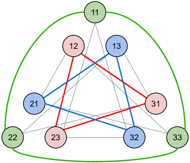
Figure 2: The triangle gadget for $2$ valid $3$-colorings. There are $2$ ways to partition the $9$ vertices into $3$ disjoint triangles. The highlighted triangles show the partition $\{S_{\pi}\}_{\pi\in\mathbb{S}_{3}^{+}}$.

Let

$$S_{\pi}\coloneqq\left\{(\sigma,\pi(\sigma)):\sigma\in\{1,2,3\}\right\}\,.$$

Then, for any $\pi\in\mathbb{S}_{3}$, $\operatorname{agree}_{\pi}(x,y)=\mathsf{wt}(S_{\pi})$.

Claim 2.6.

If $\lambda_{2}\leqslant 1-\frac{1}{1+\varepsilon}$, then,

$$\sum_{\pi\in\mathbb{S}_{3}}\mathsf{wt}(S_{\pi})^{2}\geqslant 2-\frac{1}{1-\lambda_{2}}\geqslant 1-\varepsilon\,.$$ (2)

Proof.

Observe that for any $\pi$, $S_{\pi}$ forms a triangle in $H$. In fact, there are exactly two ways to partition the $9$ vertex graph above into $3$ disjoint triangles: (1) $\{11,22,33\}$, $\{12,23,31\}$, $\{13,21,32\}$ (highlighted in Figure 2), and (2) $\{11,23,32\}$, $\{12,21,33\}$, $\{13,22,31\}$, where each of the $6$ triangles appearing in the list above corresponds to a permutation $\pi\in\mathbb{S}_{3}$.

Now, $e(S_{\pi},\overline{S}_{\pi})\geqslant(1-\lambda_{2})\cdot\mathsf{wt}(S_{\pi})(1-\mathsf{wt}(S_{\pi}))$ for each $\pi$. Summing up the inequalities over $\pi\in\mathbb{S}_{3}$ gives $(1-\lambda_{2})\sum_{\pi}\mathsf{wt}(S_{\pi})(1-\mathsf{wt}(S_{\pi}))=(1-\lambda_{2})(2-\sum_{\pi}\mathsf{wt}(S_{\pi})^{2})$ on the right-hand side and $\sum_{\pi}e(S_{\pi},\overline{S}_{\pi})=1$ on the left-hand side. Thus, rearranging gives us

$$\sum_{\pi\in\mathbb{S}_{3}}\mathsf{wt}(S_{\pi})^{2}\geqslant 2-\frac{1}{1-\lambda_{2}}\geqslant 1-\varepsilon\,.\qed$$

Small agreement + expansion implies almost bipartite.

We show the following claim:

Claim 2.7.

Suppose $\lambda_{2}\leqslant\frac{\varepsilon}{1+\varepsilon}$ and $\operatorname{agree}(x,y)\leqslant\frac{1}{2}+\varepsilon$ for small enough $\varepsilon$, then one of $\{w(S_{\pi})\}_{\pi\in\mathbb{S}_{3}^{+}}$ and one of $\{w(S_{\pi})\}_{\pi\in\mathbb{S}_{3}^{-}}$ is at most $O(\varepsilon)$.

As a result, $G$ is almost bipartite, i.e., removing an $O(\varepsilon)$ fraction of vertices results in a bipartite graph.

Recall that $\operatorname{agree}(x,y)\leqslant\frac{1}{2}+\varepsilon$ means that $\mathsf{wt}(S_{\pi})\leqslant\frac{1}{2}+\varepsilon$ for all $\pi\in\mathbb{S}_{3}$. To prove Claim 2.7, we formulate it as a $6$-variable lemma (see Lemma 5.8): let $z_{1},z_{2},\dots,z_{6}$ be such that $0\leqslant z_{i}\leqslant\frac{1}{2}+\varepsilon$ for each $i$, $z_{1}+z_{2}+z_{3}=z_{4}+z_{5}+z_{6}=1$, and $\|z\|_{2}^{2}\geqslant 1-\varepsilon$, then one of $z_{1},z_{2},z_{3}$ and one of $z_{4},z_{5},z_{6}$ must be $\leqslant O(\varepsilon)$.

With this lemma, the first statement in Claim 2.7 immediate follows from $\mathsf{wt}(S_{\pi})\leqslant\frac{1}{2}+\varepsilon$, $\sum_{\pi\in\mathbb{S}_{3}^{+}}\mathsf{wt}(S_{\pi})=\sum_{\pi\in\mathbb{S}_{3}^{-}}\mathsf{wt}(S_{\pi})=1$, and Eq. 2.

For the second statement, let $\pi^{+}\in\mathbb{S}_{3}^{+}$ and $\pi^{-}\in\mathbb{S}_{3}^{-}$ be the permutations such that $\mathsf{wt}(S_{\pi^{+}})$, $\mathsf{wt}(S_{\pi^{-}})\leqslant O(\varepsilon)$. Note that since $\pi^{+}$ and $\pi^{-}$ have different signs, $S_{\pi^{+}}$ and $S_{\pi^{-}}$ intersect in exactly one string $\alpha\in[3]^{2}$. In fact, $\alpha$ uniquely determines $\pi^{+},\pi^{-}$ since there are exactly two permutations with different signs that map $\alpha_{1}$ to $\alpha_{2}$. Assume without loss of generality (due to symmetry) that $\alpha=11$, so that $S_{\pi^{+}}=\{11,22,33\}$ and $S_{\pi^{-}}=\{11,23,32\}$. Then, we have $\mathsf{wt}(\{11,22,33\})$, $\mathsf{wt}(\{11,23,32\})\leqslant O(\varepsilon)$. This means that $\mathsf{wt}(\{12,13,21,23\})\geqslant 1-O(\varepsilon)$. Observe that $\{12,13,21,23\}$ forms a bipartite structure between $\{12,13\}$ and $\{21,23\}$, as shown in Figure 3. In particular, the first coloring labels the entire left side with the same color, while the second labels the right side with the same color.

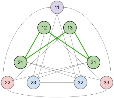
Figure 3: $S_{\pi^{+}}=\{11,22,33\}$ and $S_{\pi^{-}}=\{11,23,32\}$, and $\mathsf{wt}(S_{\pi^{+}})$, $\mathsf{wt}(S_{\pi^{-}})\leqslant O(\varepsilon)$, which means that $\mathsf{wt}(\{12,13,21,23\})\geqslant 1-O(\varepsilon)$. Here $\{12,13,21,23\}$ forms a bipartite structure.

Agreement between $3$ valid $3$-colorings.

Naturally, we consider the graph as being partitioned into $27$ subsets indexed by strings $[3]^{3}$. Again, we will use “$*$” to denote “free” coordinate, so for example $11*$ means $\{111,112,113\}$, i.e., the set $11$ if we ignore the third coloring.

Suppose for contradiction that the agreement between each pair of $3$-colorings is at most $\frac{1}{2}+\varepsilon$. Then, by Claim 2.7, we have that each pair $(i,j)$ of colorings gives a bipartite structure, denoted $T^{(ij)}$, such that $\mathsf{wt}(T^{(ij)})\geqslant 1-O(\varepsilon)$. This is best explained by example. Suppose $T^{(12)}=\{12*,13*,21*,23*\}$, $T^{(13)}=\{1*2,1*3,2*1,3*1\}$ and $T^{(23)}=\{*11,*13,*22,*32\}$. Then, we can see that $T\coloneqq T^{(12)}\cap T^{(13)}\cap T^{(23)}=\{122,132,211,311\}$. This is a bipartite structure between $\{122,132\}$ and $\{211,311\}$, where the first coloring labels the entire left side with the same color, while the second and third label the right side with the same color.

Moreover, we have $\mathsf{wt}(T)\geqslant 1-O(\varepsilon)$. We now use this to derive a contradiction. Suppose no colors have size larger than $(\frac{1}{2}+\varepsilon)n$, so $\mathsf{wt}(\{122,132\})$, $\mathsf{wt}(\{211,311\})\leqslant\frac{1}{2}+\varepsilon$. This implies that $\mathsf{wt}(\{122,132\})$, $\mathsf{wt}(\{211,311\})\geqslant\frac{1}{2}-O(\varepsilon)$. Next, observe that $\{122,211,311\}\subseteq\{*11,*22\}\subseteq S_{\pi}$ between the second and third colorings for some $\pi$. Similarly, $\{132,211,311\}\subseteq\{*11,*32\}\subseteq S_{\pi^{\prime}}$ for some $\pi^{\prime}$. Thus, one of them has weight at least $\mathsf{wt}(\{211,311\})+\frac{1}{2}\mathsf{wt}(\{122,132\})\geqslant\frac{3}{4}-O(\varepsilon)$, contradicting that each pairwise agreement is $\leqslant\frac{1}{2}+\varepsilon$.

One can verify that the above holds in general; $T$ will contain at most $4$ strings in $[3]^{3}$ and form the bipartite structure explained above. This proves Lemma 2.4.

3 Preliminaries

Notations.   For any integer $N$, we write $[N]\coloneqq\{1,2,\dots,N\}$. We will use boldface ${\bm{x}}$ to denote a collection of vectors: ${\bm{x}}=(x^{(1)},x^{(2)},\dots,x^{(t)})$. For a graph $G=(V,E)$ and a subset $S\subseteq V$, we denote the neighbors of $S$ (a.k.a. outer boundary) as $N_{G}(S)\coloneqq\{u\notin S:\exists v\in S,(u,v)\in E\}$, and the neighborhood of $S$ as $\Gamma_{G}(S)\coloneqq S\cup N_{G}(S)$. We use $\lambda_{2}(G)$ to denote the second eigenvalue of the normalized adjacency matrix $D_{G}^{-1/2}A_{G}D_{G}^{-1/2}$. The Laplacian $L_{G}$ is the matrix $D_{G}-A_{G}$ where $D_{G}$ is the diagonal degree matrix and $A_{G}$ is the adjacency matrix. We use $\widetilde{L}_{G}$ to denote the normalized Laplacian. In all of the above, we drop the dependence on $G$ if it is clear from context.

3.1 Background on Sum-of-Squares

We refer the reader to the monograph [FKP19] and the lecture notes [BS16] for a detailed exposition of the sum-of-squares method and its usage in algorithm design.

Pseudodistributions.   Pseudodistributions are generalizations of probability distributions. Formally, a pseudodistribution on $\mathbb{R}^{n}$ is a finitely supported signed measure $\mu:\mathbb{R}^{n}\rightarrow\mathbb{R}$ such that $\sum_{x}\mu(x)=1$. The associated pseudo-expectation is a linear operator $\widetilde{\mathbb{E}}_{\mu}$ that assigns to every polynomial $f:\mathbb{R}^{n}\rightarrow\mathbb{R}$ the value $\widetilde{\mathbb{E}}_{\mu}f=\sum_{x}\mu(x)f(x)$, which we call the pseudo-expectation of $f$. We say that a pseudodistribution $\mu$ on $\mathbb{R}^{n}$ has degree $d$ if $\widetilde{\mathbb{E}}_{\mu}[f^{2}]\geqslant 0$ for every polynomial $f$ on $\mathbb{R}^{n}$ of degree $\leqslant d/2$.

A degree-$d$ pseudodistribution $\mu$ is said to satisfy a constraint $\{q(x)\geqslant 0\}$ for any polynomial $q$ of degree $\leqslant d$ if for every polynomial $p$ such that $\deg(p^{2})\leqslant d-\deg(q)$, $\widetilde{\mathbb{E}}_{\mu}[p^{2}q]\geqslant 0$. For example, in this work we will often say that $\mu$ satisfies the Booleanity constraints $\{x_{i}^{2}-x_{i}=0,\ \forall i\in[n]\}$, which means that $\widetilde{\mathbb{E}}_{\mu}[p(x)(x_{i}^{2}-x_{i})]=0$ for any $i$ and any polynomial $p$ of degree $d-2$. We say that $\mu$ $\tau$-approximately satisfies a constraint $\{q\geqslant 0\}$ if for any sum-of-squares polynomial $p$, $\widetilde{\mathbb{E}}_{\mu}[pq]\geqslant-\tau\left\lVert p\right\rVert_{2}$ where $\left\lVert p\right\rVert_{2}$ is the $\ell_{2}$ norm of the coefficient vector of $p$.

We rely on the following basic connection that forms the basis of the sum-of-squares algorithm.

Fact 3.1 (Sum-of-Squares algorithm, [Par00, Las01]).

Given a system of degree $\leqslant d$ polynomial constraints $\{q_{i}\geqslant 0\}$ in $n$ variables and the promise that there is a degree-$d$ pseudodistribution satisfying $\{q_{i}\geqslant 0\}$ as constraints, there is a $n^{O(d)}\operatorname{polylog}(1/\tau)$ time algorithm to find a pseudodistribution of degree $d$ on $\mathbb{R}^{n}$ that $\tau$-approximately satisfies the constraints $\{q_{i}\geqslant 0\}$.

Sum-of-squares proofs.

Let $f_{1},f_{2},\dots,f_{m}$ and $g$ be multivariate polynomials in $x$. A sum-of-squares proof that the constraints $\{f_{1}\geqslant 0,\dots,f_{m}\geqslant 0\}$ imply $g\geqslant 0$ consists of sum-of-squares polynomials $(p_{S})_{S\subseteq[m]}$ such that $g=\sum_{S\subseteq[m]}p_{S}\prod_{i\in S}f_{i}$. The degree of such a sum-of-squares proof equals the maximum of the degree of $p_{S}\prod_{i\in S}f_{i}$ over all $S$ appearing in the sum above. We write $\{f_{i}\geqslant 0,\ \forall i\in[m]\}\mathrel{\leavevmode\hbox{\set@color\raisebox{3.44444pt}{$\rule[-6.45831pt]{0.47787pt}{12.91663pt}\rule[-0.23894pt]{8.00063pt}{0.47787pt}\raisebox{-6.82222pt}{\makebox[8.00063pt]{\leavevmode\hbox{\set@color$\scriptstyle{d}$}}}\raisebox{1.96112pt}{\makebox[8.00063pt]{\leavevmode\hbox{\set@color$\scriptstyle{x}$}}}$}}}\{g\geqslant 0\}$ where $d$ is the degree of the sum-of-squares proof.

We will rely on the following basic connection between SoS proofs and pseudodistributions:

Fact 3.2.

Let $f_{1},\dots,f_{m}$ and $g$ be polynomials, and let $\mathcal{A}=\{f_{i}(x)\geqslant 0,\ \forall i\in[m]\}$. Suppose $\mathcal{A}\mathrel{\leavevmode\hbox{\set@color\raisebox{3.44444pt}{$\rule[-6.45831pt]{0.47787pt}{12.91663pt}\rule[-0.23894pt]{8.00063pt}{0.47787pt}\raisebox{-6.82222pt}{\makebox[8.00063pt]{\leavevmode\hbox{\set@color$\scriptstyle{d}$}}}\raisebox{1.96112pt}{\makebox[8.00063pt]{\leavevmode\hbox{\set@color$\scriptstyle{x}$}}}$}}}\{g(x)\geqslant 0\}$. Then, for any pseudodistribution $\mu$ of degree $\geqslant d$ satisfying $\mathcal{A}$, we have $\widetilde{\mathbb{E}}_{\mu}[g]\geqslant 0$.

Therefore, an SoS proof of some polynomial inequality directly implies that the same inequality holds in pseudoexpectation. We will use this repeatedly in our analysis.

SoS toolkit.

The theory of univariate sum-of-squares (in particular, Lukács Theorem) says that if a univariate polynomial is non-negative on an interval, then this fact is also SoS-certifiable. The following corollary of Lukács theorem is well-known, and we will use it multiple times to convert univariate inequalities into SoS inequalities in a blackbox manner.

Fact 3.3 (Corollary of Lukács Theorem).

Let $a\leqslant b\in\mathbb{R}$. Let $p\in\mathbb{R}[x]$ be a univariate real polynomial of degree $d$ such that $p(x)\geqslant 0$ for all $a\leqslant x\leqslant b$. Then,

$$\left\{x\geqslant a,\ x\leqslant b\right\}\mathrel{\leavevmode\hbox{\set@color\raisebox{3.44444pt}{$\rule[-6.45831pt]{0.47787pt}{12.91663pt}\rule[-0.23894pt]{8.00063pt}{0.47787pt}\raisebox{-6.82222pt}{\makebox[8.00063pt]{\leavevmode\hbox{\set@color$\scriptstyle{d}$}}}\raisebox{1.96112pt}{\makebox[8.00063pt]{\leavevmode\hbox{\set@color$\scriptstyle{x}$}}}$}}}\left\{p(x)\geqslant 0\right\}\,.$$

Similarly, true inequalities on the hypercube are also SoS-certifiable.

Fact 3.4.

Let $p$ be a polynomial in $n$ variables. Suppose $p(x)\geqslant 0$ for all $x\in\{0,1\}^{n}$, then

$$\left\{x_{i}^{2}-x_{i}=0,\ \forall i\in[n]\right\}\mathrel{\leavevmode\hbox{\set@color\raisebox{3.44444pt}{$\rule[-6.45831pt]{0.47787pt}{12.91663pt}\rule[-0.23894pt]{48.08464pt}{0.47787pt}\raisebox{-7.21112pt}{\makebox[48.08464pt]{\leavevmode\hbox{\set@color$\scriptstyle{\max(n,\deg(p))}$}}}\raisebox{1.96112pt}{\makebox[48.08464pt]{\leavevmode\hbox{\set@color$\scriptstyle{x}$}}}$}}}\left\{p(x)\geqslant 0\right\}\,.$$

More generally, all true inequalities have SoS certificates under mild assumptions. In particular, Schmüdgen’s Positivstellensatz establishes the completeness of the SoS proof system under compactness conditions (often called the Archimedean condition). Moreover, bounds on the SoS degree (given the polynomial and the constraints) were given in [PD01, Sch04].

Fact 3.5 (Positivstellensatz [PD01, Sch04]).

For all polynomials $g_{1},g_{2},\dots,g_{m}$ over $x=(x_{1},x_{2},\dots,x_{n})$ defining a non-empty set

$$S\coloneqq\{x\in\mathbb{R}^{n}:g_{1}(x)\geqslant 0,\dots,g_{m}(x)\geqslant 0\}\subseteq(-1,1)^{n}\,,$$

and for every polynomial $f$ of degree $d$ with coefficients bounded by $R$ and $f^{*}\coloneqq\min_{x\in S}f(x)>0$, there exists an integer $D=D(n,g_{1},\dots,g_{m},R,f^{*})\in\mathbb{N}$ such that

$$\left\{g_{1}\geqslant 0,\dots,g_{m}\geqslant 0\right\}\mathrel{\leavevmode\hbox{\set@color\raisebox{3.44444pt}{$\rule[-6.45831pt]{0.47787pt}{12.91663pt}\rule[-0.23894pt]{9.98979pt}{0.47787pt}\raisebox{-6.74445pt}{\makebox[9.98979pt]{\leavevmode\hbox{\set@color$\scriptstyle{D}$}}}\raisebox{1.96112pt}{\makebox[9.98979pt]{\leavevmode\hbox{\set@color$\scriptstyle{x}$}}}$}}}\left\{f\geqslant 0\right\}\,.$$

Independent samples from a pseudodistribution.

Recall that a given pseudoexpectation operator $\widetilde{\mathbb{E}}_{\mu}$ has the interpretation as averaging of functions $f(x)$ over a pseudodistribution $x\sim\mu$. We will need to be able to mimic averaging over $t$ independently chosen samples $x^{(1)},\ldots,x^{(t)}\sim\mu$. We define the product pseudodistribution $\mu^{\otimes t}$ along with pseudoexpectation $\widetilde{\mathbb{E}}_{\mu^{\otimes t}}$ as follows: let $p({\bm{x}})=(x^{(1)})^{\alpha_{1}}\ldots(x^{(t)})^{\alpha_{t}}$ be a monomial in variables ${\bm{x}}=(x^{(1)},\ldots,x^{(t)})$; we define

$$\widetilde{\mathbb{E}}_{\mu^{\otimes t}}[p]:=\widetilde{\mathbb{E}}_{\mu}[x^{\alpha_{1}}]\cdot\widetilde{\mathbb{E}}_{\mu}[x^{\alpha_{2}}]\cdots\widetilde{\mathbb{E}}_{\mu}[x^{\alpha_{t}}]\,.$$

It is easy to check that $\widetilde{\mathbb{E}}_{\mu^{\otimes t}}$ is also a pseudoexpectation operator corresponding to $t$ independent samples from the pseudodistribution $\mu$.

Fact 3.6.

If $\widetilde{\mathbb{E}}_{\mu}$ is a valid pseudodistribution of degree $D$ in variables $x$, then $\widetilde{\mathbb{E}}_{\mu^{\otimes t}}$ is a valid pseudodistribution of degree $D$. Furthermore, if additional SoS inequalities are true for $\widetilde{\mathbb{E}}_{\mu}$, they also hold for $\widetilde{\mathbb{E}}_{\mu^{\otimes t}}$.

3.2 Basic Facts on Independent Sets

The following is the well-known $2$-approximation algorithm for minimum vertex cover.

Fact 3.7.

If an $n$-vertex graph $G$ has an independent set of size at least $(\frac{1}{2}+\varepsilon)n$, then there exists a polynomial-time algorithm that outputs an independent set of size at least $2\varepsilon n$.

We will also rely on the following simple fact repeatedly.

Fact 3.8.

For a graph $G=(V,E)$, let $\mu$ be a pseudodistribution of degree at least $2$ that satisfies the independent set constraints, i.e., $x_{u}^{2}=x_{u}$ for all $u\in V$ and $x_{u}x_{v}=0$ for all $\{u,v\}\in E$. Then, the set of vertices $\{u\in V:\widetilde{\mathbb{E}}_{\mu}[x_{u}]>\frac{1}{2}\}$ forms an independent set in $G$.

Proof.

For all $\{u,v\}\in E$, from the independent set constraints we can derive that $(x_{u}+x_{v})^{2}=x_{u}^{2}+2x_{u}x_{v}+x_{v}^{2}=x_{u}+x_{v}$, i.e., $(x_{u}+x_{v})$ satisfies the Booleanity constraint, thus $x_{u}+x_{v}\leqslant 1$. Thus, we have $\widetilde{\mathbb{E}}_{\mu}[x_{u}+x_{v}]\leqslant 1$, which means that $u,v$ cannot both be in the set $\{u\in V:\widetilde{\mathbb{E}}_{\mu}[x_{u}]>\frac{1}{2}\}$. ∎

3.3 Information Theory

We will use $\mu|_{R}$ to denote the marginal distribution of a random variable $R\sim\mu$. We use $TV(X,Y)$ to denote the total-variation distance between two distributions $X,Y$.

Definition 3.9 (Mutual Information).

Given a distribution $\mu$ over $(X,Y)$, the mutual information between $X,Y$ is defined as:

$$I_{\mu}(X;Y)=D_{KL}(\mu~{}||~{}\mu|_{X}\times\mu|_{Y}),$$

where $D_{KL}$ is the Kullback-Leibler divergence. We drop $\mu$ from the subscript when the distribution is clear from context. The conditional mutual information between $(X,Y)$ with respect to a random variable $Z$ is defined as:

$$I(X;Y|Z)=\mathbb{E}_{z\sim Z}[I_{\mu|Z=z}(X;Y)].$$

Fact 3.10 (Pinsker’s inequality).

Given any two distributions $D_{1},D_{2}$:

$$TV(D_{1},D_{2})\leqslant\sqrt{\frac{1}{2}D_{KL}(D_{1}||D_{2})}.$$

3.4 Conditioning Pseudodistributions

We can reweigh or condition a degree-$D$ pseudodistribution $\mu$ by a polynomial $s(x)$, where $s(x)$ is non-negative under the program axioms, i.e., $\mathcal{A}\mathrel{\leavevmode\hbox{\set@color\raisebox{3.44444pt}{$\rule[-6.45831pt]{0.47787pt}{12.91663pt}\rule[-0.23894pt]{8.00063pt}{0.47787pt}\raisebox{-6.82222pt}{\makebox[8.00063pt]{\leavevmode\hbox{\set@color$\scriptstyle{d}$}}}\raisebox{1.96112pt}{\makebox[8.00063pt]{\leavevmode\hbox{\set@color$\scriptstyle{x}$}}}$}}}\{s(x)\geqslant 0\}$ for $d<D$. Technically, this operation defines a new pseudodistribution $\mu^{\prime}$ of degree $D-d$ with pseudoexpectation operator $\widetilde{\mathbb{E}}_{\mu^{\prime}}$ by taking

$$\widetilde{\mathbb{E}}_{\mu^{\prime}}[x^{\alpha}]=\frac{\widetilde{\mathbb{E}}_{\mu}[x^{\alpha}\cdot s(x)]}{\widetilde{\mathbb{E}}_{\mu}[s(x)]}\,,$$

for every monomial $x^{\alpha}$ of degree at most $D-d$.

It is easy to verify that $\mu^{\prime}$ is a valid pseudodistribution of degree $D-d$ and satisfies the axioms of the original $\mu$. As an example, under the independent set axioms presented in (1), since $x_{i}\geqslant 0$ is an axiom, one can reweigh $\mu$ by $x_{i}$, essentially “conditioning” the pseudodistribution on the event $x_{i}=1$. Thus, we will also refer to this operation as conditioning and denote $\mu^{\prime}$ by $\mu|s(x)$. Often times, the polynomial $s(x)$ we will “condition” on will be a polynomial approximation of the indicator function of some event $E$. In this case, the above operation can be interpreted as conditioning $\mu$ to satisfy some properties specified by the event $E$.

Approximate polynomials to indicator functions.

Our arguments require indicators of events such as $f(x)\geqslant\delta$ where $f$ is a low-degree polynomial, and we will need to condition on such events. Strictly speaking, the function $\bm{1}[f(x)\geqslant\delta]$ is not a low-degree polynomial and therefore we cannot condition on it. However, it is not difficult to show that such indicators can be approximated by low-degree polynomials, and in particular we use the the following result, due to [DGJ⁺10], that provides a low-degree approximation to a step function.

Lemma 3.11.

For every $0<\nu<\delta<1$, there is a univariate polynomial $Q_{\delta,\nu}$ of degree $O(\frac{1}{\nu}\log^{2}\frac{1}{\nu})$ such that:

1. $Q_{\delta,\nu}(x)\in[0,\nu]$ for all $x\in[0,\delta-\nu]$.

2. $Q_{\delta,\nu}(x)\in[1,1+\nu]$ for all $x\in[\delta,1]$.

3. $Q_{\delta,\nu}$ is monotonically increasing on $(\delta-\nu,\delta)$.

Furthermore, all these facts are SoS-certifiable in degree $\deg(Q_{\delta,\nu})$.

Reducing average correlation.

An important technique we need is reducing the average correlation of random variables through conditioning, which was introduced in [BRS11] (termed global correlation reduction) and is also applicable to pseudodistributions of sufficiently large degree. We will use the following version from [RT12].

Lemma 3.12.

Let $Y_{1},\ldots,Y_{M}$ be a set of random variables each taking values in $\{1,\ldots,q\}$. Then, for any $\ell\in\mathbb{N}$, there exists $k\leqslant\ell$ such that:

$$\mathbb{E}_{i_{1},\ldots,i_{k}\sim[M]}\mathbb{E}_{i,j\sim[M]}[I(Y_{i};Y_{j}\mid Y_{i_{1}},\ldots,Y_{i_{k}})]\leqslant\frac{\log q}{\ell-1}.$$

Note that the above lemma holds as long as there is a local collection of distributions over $(Y_{1},\ldots,Y_{M})$ that are valid probability distributions over all collections of $\ell+2$ variables and are consistent with each other. Of particular interest to us would be the setting where we have a degree $\geqslant\ell+2$-pseudodistribution $\mu$ over the variables $(Y_{1},\ldots,Y_{M})$.

We also require a generalization of the above lemma to $t$-wise correlations.

Lemma 3.13 (Lemma 32 of [MR17]).

Let $Y_{1},\ldots,Y_{M}$ be a set of random variables each taking values in $\{1,\ldots,q\}$. The total $t$-wise correlation of a distribution $\mu$ over $Y_{1},\dots,Y_{M}$ is defined as

$$\operatorname{TC}_{t}(\mu)\coloneqq\mathbb{E}_{i_{1},\dots,i_{t}\sim[M]}\left[\operatorname{KL}((Y_{i_{1}},\dots,Y_{i_{t}})\|Y_{i_{1}}\times\cdots\times Y_{i_{t}})\right]\,.$$

Then, for any $\ell\in\mathbb{N}$, there exists $k\leqslant\ell$ such that:

$$\mathbb{E}_{\begin{subarray}{c}i_{1},\ldots,i_{k}\sim[M]\\ (y_{i_{1}},\ldots,y_{i_{k}})\sim\mu\end{subarray}}[\operatorname{TC}_{t}(\mu\mid Y_{i_{1}}=y_{i_{1}},\ldots,Y_{i_{k}}=y_{i_{k}})]\leqslant\frac{t^{2}\log q}{\ell}\,.$$

Similar to Lemma 3.12, the above holds for pseudodistributions of degree $\geqslant\ell+t$.

4 Independent Sets on Spectral Expanders

We prove the following theorem in this section:

Theorem 4.1 (Restatement of Theorem 2).

There is a polynomial-time algorithm that, given an $n$-vertex regular graph $G$ that contains an independent set of size $(\frac{1}{2}-\varepsilon)n$ and has $\lambda_{2}(G)\leqslant 1-40\varepsilon$ for any $\varepsilon\leqslant 0.001$, outputs an independent set of size at least $n/1000$.

Our algorithm starts by considering a constant degree SoS relaxation of the integer program for Independent Set (1) and obtaining a pseudodistribution $\mu^{\prime}$. We then apply a simple rounding algorithm to obtain an independent set in $G$ as shown below.

Algorithm 1 (Find independent set in an expander).

Input: A graph $G=(V,E)$. Output: An independent set of $G$. Operation: 1. Solve the SoS relaxation of degree $D=O(1)$ of the integer program (1) to obtain a pseudodistribution $\mu^{\prime}$. 2. Choose a uniformly random set of $t=O(1)$ vertices $i_{1},\ldots,i_{t}\sim[n]$ and draw $(\sigma_{i_{1}},\ldots,\sigma_{i_{t}})\sim\mu^{\prime}$. Let $\mu$ be the pseudodistribution obtained by conditioning $\mu^{\prime}$ on
$(x_{i_{1}}=\sigma_{i_{1}},\ldots,x_{i_{t}}=\sigma_{i_{t}})$. 3. Output the set $\{u\in V:\widetilde{\mathbb{E}}_{\mu}[x_{u}]>\frac{1}{2}\}$.

4.1 Multiple Assignments from $\mu$: Definitions and Facts

Fix $t\in\mathbb{N}$. Throughout this section, we will work with $t$ assignments $x^{(1)},x^{(2)},\dots,x^{(t)}$ that the reader should think of as independent samples from the pseudodistribution $\mu$, i.e. each $x^{(i)}$ is an $n$-dimensional vector which is the indicator of a $(1/2-\varepsilon)n$-sized independent set in $G$ and therefore it satisfies the constraints of the integer program (1). Given $x^{(1)},x^{(2)},\dots,x^{(t)}$ we use boldface ${\bm{x}}$ to denote $(x^{(1)},\dots,x^{(t)})$, i.e., the collection of variables $x_{u}^{(i)}$ for $u\in[n]$ and $i\in[t]$. Moreover, for $U\subseteq[t]$, we write ${\bm{x}}^{U}\coloneqq(x^{(i)})_{i\in U}$.

Definition 4.2.

We denote $\mathcal{A}^{\mathsf{bool}}_{G}(x)\coloneqq\{x_{u}^{2}-x_{u}=0,\ \forall u\in V\}$, i.e., the Booleanity constraints. Moreover, we write $\mathcal{A}^{\mathsf{IS}}_{G}(x)$ to denote the independent set constraints:

$$\mathcal{A}^{\mathsf{IS}}_{G}(x)\coloneqq\mathcal{A}^{\mathsf{bool}}_{G}(x)\cup\{x_{u}x_{v}=0,\ \forall\{u,v\}\in E\}\,.$$

Moreover, with slight abuse of notation, for $t\in\mathbb{N}$ and vectors $x^{(1)},x^{(2)},\dots,x^{(t)}$,

$$\mathcal{A}^{\mathsf{bool}}_{G}({\bm{x}})\coloneqq\bigcup_{i\in[t]}\mathcal{A}^{\mathsf{bool}}_{G}(x^{(i)})\,,\quad\mathcal{A}^{\mathsf{IS}}_{G}({\bm{x}})\coloneqq\bigcup_{i\in[t]}\mathcal{A}^{\mathsf{IS}}_{G}(x^{(i)})\,.$$

We will drop the dependence on $G$ when the graph is clear from context.

Given assignments $x^{(1)},\dots,x^{(t)}\in\{0,1\}^{n}$ and $\alpha\in\{0,1\}^{t}$, for each vertex $u\in[n]$, we define below the event that $u$ is assigned $\alpha_{i}$ by $x^{(i)}$, which is viewed as a degree-$t$ multilinear polynomial of ${\bm{x}}$. Similarly, for $S\subseteq\{0,1\}^{t}$, we define the event that $u$ receives one of the assignments in $S$.

Definition 4.3.

Let $t\in\mathbb{N}$, and let ${\bm{x}}=(x^{(1)},x^{(2)},\dots,x^{(t)})$. For each $u\in[n]$, $\alpha\in\{0,1\}^{t}$ and $S\subseteq\{0,1\}^{t}$, we define the following events,

$$\bm{1}(u\leftarrow\alpha)\coloneqq\bm{1}(x_{u}^{(1)}=\alpha_{1},\ldots,x_{u}^{(t)}=\alpha_{t})=\prod_{i\in[t]}\left(x_{u}^{(i)}\right)^{\alpha_{i}}\left(1-x_{u}^{(i)}\right)^{1-\alpha_{i}}\,,$$

$$\bm{1}(u\leftarrow S)\coloneqq\sum_{\alpha\in S}\bm{1}(u\leftarrow\alpha)\,.$$

For convenience, we omit the dependence on ${\bm{x}}$. We will also consider the quantity $\mathsf{wt}(\alpha)$ which is the fraction of vertices that get assigned $\alpha$:

$$\mathsf{wt}(\alpha)\coloneqq\mathbb{E}_{u\in[n]}[\bm{1}(u\leftarrow\alpha)]\,.$$

Similarly, $\mathsf{wt}(S)\coloneqq\mathbb{E}_{u\in[n]}[\bm{1}(u\leftarrow S)]$ for $S\subseteq\{0,1\}^{t}$.

Moreover, we will use the symbol “$*$” to denote “free variables” — for $\beta\in\{0,1,*\}^{t}$, $\bm{1}(u\leftarrow\beta)\coloneqq\bm{1}(u\leftarrow S_{\beta})$ and $\mathsf{wt}(\beta)\coloneqq\mathsf{wt}(S_{\beta})$ where $S_{\beta}=\{\alpha\in\{0,1\}^{t}:\alpha_{i}=\beta_{i}\text{ if }\beta_{i}\neq*\}$. For example, $\mathsf{wt}(00*)=\mathsf{wt}(000)+\mathsf{wt}(001)$.

We note some simple facts (written in SoS form) that will be useful later.

Fact 4.4.

The following can be easily verified:

1. $\mathcal{A}^{\mathsf{bool}}({\bm{x}})\mathrel{\leavevmode\hbox{\set@color\raisebox{3.44444pt}{$\rule[-6.45831pt]{0.47787pt}{12.91663pt}\rule[-0.23894pt]{10.02773pt}{0.47787pt}\raisebox{-6.47223pt}{\makebox[10.02773pt]{\leavevmode\hbox{\set@color$\scriptstyle{2t}$}}}\raisebox{1.96112pt}{\makebox[10.02773pt]{\leavevmode\hbox{\set@color$\scriptstyle{{\bm{x}}}$}}}$}}}\left\{\bm{1}(u\leftarrow\alpha)^{2}=\bm{1}(u\leftarrow\alpha)\right\}$, i.e., $\bm{1}(u\leftarrow\alpha)$ satisfies the Booleanity constraint.

2. $\mathcal{A}^{\mathsf{bool}}({\bm{x}})\mathrel{\leavevmode\hbox{\set@color\raisebox{3.44444pt}{$\rule[-6.45831pt]{0.47787pt}{12.91663pt}\rule[-0.23894pt]{10.02773pt}{0.47787pt}\raisebox{-6.47223pt}{\makebox[10.02773pt]{\leavevmode\hbox{\set@color$\scriptstyle{2t}$}}}\raisebox{1.96112pt}{\makebox[10.02773pt]{\leavevmode\hbox{\set@color$\scriptstyle{{\bm{x}}}$}}}$}}}\left\{\bm{1}(u\leftarrow\alpha)\cdot\bm{1}(u\leftarrow\beta)=0\right\}$ for $\alpha\neq\beta$. This also implies that $\bm{1}(u\leftarrow S)$ satisfies the Booleanity constraint for any $S\subseteq\{0,1\}^{t}$.

3. $\mathrel{\leavevmode\hbox{\set@color\raisebox{3.44444pt}{$\rule[-6.45831pt]{0.47787pt}{12.91663pt}\rule[-0.23894pt]{8.00063pt}{0.47787pt}\raisebox{-6.26668pt}{\makebox[8.00063pt]{\leavevmode\hbox{\set@color$\scriptstyle{t}$}}}\raisebox{1.96112pt}{\makebox[8.00063pt]{\leavevmode\hbox{\set@color$\scriptstyle{{\bm{x}}}$}}}$}}}\left\{\sum_{\alpha\in\{0,1\}^{t}}\bm{1}(u\leftarrow\alpha)=1\right\}$.

We next prove the following lemma, which is an “SoS proof” that if $x^{(1)},\dots,x^{(t)}$ are indicators of independent sets and $\{u,v\}\in E$, then $u$ and $v$ cannot be both assigned $1$ by any $x^{(i)}$. As a consequence, any vertex that is assigned all $1$s can only be connected to vertices that are assigned all $0$s, meaning that if $v$ gets $\vec{1}$ then $u$ must get $\vec{0}$.

Lemma 4.5.

Let $t\in\mathbb{N}$ and ${\bm{x}}=(x^{(1)},x^{(2)},\dots,x^{(t)})$ be variables. For any graph $G=(V,E)$ and any $\alpha,\beta\in\{0,1\}^{t}$ such that $\mathrm{supp}(\alpha)\cap\mathrm{supp}(\beta)\neq\varnothing$, then for all $\{u,v\}\in E$ we have

$$\mathcal{A}^{\mathsf{IS}}_{G}({\bm{x}})\mathrel{\leavevmode\hbox{\set@color\raisebox{3.44444pt}{$\rule[-6.45831pt]{0.47787pt}{12.91663pt}\rule[-0.23894pt]{10.02773pt}{0.47787pt}\raisebox{-6.47223pt}{\makebox[10.02773pt]{\leavevmode\hbox{\set@color$\scriptstyle{2t}$}}}\raisebox{1.96112pt}{\makebox[10.02773pt]{\leavevmode\hbox{\set@color$\scriptstyle{{\bm{x}}}$}}}$}}}\left\{\bm{1}(u\leftarrow\alpha)\bm{1}(v\leftarrow\beta)=0\right\}\,.$$

In particular, for all $\{u,v\}\in E$,

$$\mathcal{A}^{\mathsf{IS}}_{G}({\bm{x}}) \mathrel{\leavevmode\hbox{\set@color\raisebox{3.44444pt}{$\rule[-6.45831pt]{0.47787pt}{12.91663pt}\rule[-0.23894pt]{10.02773pt}{0.47787pt}\raisebox{-6.47223pt}{\makebox[10.02773pt]{\leavevmode\hbox{\set@color$\scriptstyle{2t}$}}}\raisebox{1.96112pt}{\makebox[10.02773pt]{\leavevmode\hbox{\set@color$\scriptstyle{{\bm{x}}}$}}}$}}}\left\{\left(1-\bm{1}(u\leftarrow\vec{0})\right)\cdot\bm{1}(v\leftarrow\vec{1})=0\right\}$$

$$\mathrel{\leavevmode\hbox{\set@color\raisebox{3.44444pt}{$\rule[-6.45831pt]{0.47787pt}{12.91663pt}\rule[-0.23894pt]{10.02773pt}{0.47787pt}\raisebox{-6.47223pt}{\makebox[10.02773pt]{\leavevmode\hbox{\set@color$\scriptstyle{2t}$}}}\raisebox{1.96112pt}{\makebox[10.02773pt]{\leavevmode\hbox{\set@color$\scriptstyle{{\bm{x}}}$}}}$}}}\left\{\bm{1}(u\leftarrow\vec{0})\geqslant\bm{1}(v\leftarrow\vec{1})\right\}\,.$$

Proof.

Let $i\in[t]$ be the index such that $\alpha_{i}=\beta_{i}=1$. Then, by Definition 4.3, $\bm{1}(u\leftarrow\alpha)\cdot\bm{1}(v\leftarrow\beta)=x_{u}^{(i)}x_{v}^{(i)}\cdot f({\bm{x}})$ for some polynomial $f$ (not depending on $x^{(i)}$). The first statement follows since $x_{u}^{(i)}x_{v}^{(i)}=0$ is in the independent set constraints.

For the second statement, $(1-\bm{1}(u\leftarrow\vec{0}))\bm{1}(v\leftarrow\vec{1})=0$ follows from the polynomial equality $\sum_{\alpha\in\{0,1\}^{t}}\bm{1}(u\leftarrow\alpha)=1$ and that $\vec{1}$ intersects with all $\alpha\neq\vec{0}$. Moreover, $\bm{1}(u\leftarrow\alpha)$ satisfies the Booleanity constraints (Fact 4.4). Denoting $a\coloneqq\bm{1}(u\leftarrow\vec{0})$ and $b\coloneqq\bm{1}(u\leftarrow\vec{1})$ for convenience, from $(1-a)b=0$ and $a^{2}=a$, $b^{2}=b$ we have

$$a-b=(a-b)^{2}-2(1-a)b+(a-a^{2})+(b-b^{2})\geqslant 0\,,$$

which completes the proof. ∎

4.2 Spectral Gap implies a Unique Solution

Recall the definitions from Definition 4.3. We need some definitions for edge sets in the graph.

Definition 4.6.

Let $G$ be a graph, let $t\in\mathbb{N}$, and let ${\bm{x}}=(x^{(1)},\dots,x^{(t)})$. For $\alpha,\beta\in\{0,1\}^{t}$, define

$$e(\alpha,\beta)\coloneqq\frac{1}{2|E(G)|}\sum_{\{u,v\}\in E(G)}\bm{1}(u\leftarrow\alpha)\bm{1}(v\leftarrow\beta)+\bm{1}(u\leftarrow\beta)\bm{1}(v\leftarrow\alpha)\,.$$

Here, we omit the dependence on ${\bm{x}}$ and $G$ for simplicity.

Similarly, for $S,T\subseteq\{0,1\}^{t}$, we denote $e(S,T)\coloneqq\sum_{\alpha\in S}\sum_{\beta\in T}e(\alpha,\beta)$.

Given assignments $x^{(1)},\dots,x^{(t)}\in\{0,1\}^{n}$ and $\alpha,\beta\in\{0,1\}^{t}$, one should view $e(\alpha,\beta)$ as the (normalized) number of edges between vertices that are assigned $\alpha$ and vertices assigned $\beta$. We note a few properties which can be easily verified:

Fact 4.7.

The following can be easily verified:

1. Symmetry: $e(\alpha,\beta)=e(\beta,\alpha)$ by definition.

2. Sum of edge weights (double counted) equals $1$: $\mathrel{\leavevmode\hbox{\set@color\raisebox{3.44444pt}{$\rule[-6.45831pt]{0.47787pt}{12.91663pt}\rule[-0.23894pt]{10.02773pt}{0.47787pt}\raisebox{-6.47223pt}{\makebox[10.02773pt]{\leavevmode\hbox{\set@color$\scriptstyle{2t}$}}}\raisebox{1.96112pt}{\makebox[10.02773pt]{\leavevmode\hbox{\set@color$\scriptstyle{{\bm{x}}}$}}}$}}}\{\sum_{\alpha,\beta\in\{0,1\}^{t}}e(\alpha,\beta)=1\}$, which follows from $\mathrel{\leavevmode\hbox{\set@color\raisebox{3.44444pt}{$\rule[-6.45831pt]{0.47787pt}{12.91663pt}\rule[-0.23894pt]{8.00063pt}{0.47787pt}\raisebox{-6.26668pt}{\makebox[8.00063pt]{\leavevmode\hbox{\set@color$\scriptstyle{t}$}}}\raisebox{1.96112pt}{\makebox[8.00063pt]{\leavevmode\hbox{\set@color$\scriptstyle{{\bm{x}}}$}}}$}}}\{\sum_{\alpha\in\{0,1\}^{t}}\bm{1}(u\leftarrow\alpha)=1\}$.

3. For a regular graph, the weight of a subset equals the weight of incident edges: for any $\alpha\in\{0,1\}^{t}$, $\mathrel{\leavevmode\hbox{\set@color\raisebox{3.44444pt}{$\rule[-6.45831pt]{0.47787pt}{12.91663pt}\rule[-0.23894pt]{10.02773pt}{0.47787pt}\raisebox{-6.47223pt}{\makebox[10.02773pt]{\leavevmode\hbox{\set@color$\scriptstyle{2t}$}}}\raisebox{1.96112pt}{\makebox[10.02773pt]{\leavevmode\hbox{\set@color$\scriptstyle{{\bm{x}}}$}}}$}}}\{\sum_{\beta\in\{0,1\}^{t}}e(\alpha,\beta)=\mathsf{wt}(\alpha)\}$.

4. $\mathcal{A}^{\mathsf{IS}}_{G}({\bm{x}})\mathrel{\leavevmode\hbox{\set@color\raisebox{3.44444pt}{$\rule[-6.45831pt]{0.47787pt}{12.91663pt}\rule[-0.23894pt]{10.02773pt}{0.47787pt}\raisebox{-6.47223pt}{\makebox[10.02773pt]{\leavevmode\hbox{\set@color$\scriptstyle{2t}$}}}\raisebox{1.96112pt}{\makebox[10.02773pt]{\leavevmode\hbox{\set@color$\scriptstyle{{\bm{x}}}$}}}$}}}\left\{e(\alpha,\beta)=0\right\}$ for any $\alpha,\beta$ such that $\mathrm{supp}(\alpha)\cap\mathrm{supp}(\beta)\neq\varnothing$ due to Lemma 4.5.

We next show the following lemma relating the Laplacian to the cut in the graph.

Lemma 4.8.

Let $G$ be a graph and $L_{G}$ be its Laplacian matrix. Let $t\in\mathbb{N}$, $S\subseteq\{0,1\}^{t}$, and let $y_{u}\coloneqq\bm{1}(u\leftarrow S)$ for each vertex $u$, we have

$$\mathcal{A}^{\mathsf{bool}}({\bm{x}})\mathrel{\leavevmode\hbox{\set@color\raisebox{3.44444pt}{$\rule[-6.45831pt]{0.47787pt}{12.91663pt}\rule[-0.23894pt]{10.02773pt}{0.47787pt}\raisebox{-6.47223pt}{\makebox[10.02773pt]{\leavevmode\hbox{\set@color$\scriptstyle{2t}$}}}\raisebox{1.96112pt}{\makebox[10.02773pt]{\leavevmode\hbox{\set@color$\scriptstyle{{\bm{x}}}$}}}$}}}\left\{\frac{1}{2|E(G)|}\cdot y^{\top}L_{G}y=e(S,\overline{S})\right\}\,.$$

Proof.

Since $y_{u}$ satisfies the Booleanity constraint and $1-\bm{1}(u\leftarrow S)=\bm{1}(u\leftarrow\overline{S})$, for any $u,v$,

$$\mathcal{A}^{\mathsf{bool}}({\bm{x}})\mathrel{\leavevmode\hbox{\set@color\raisebox{3.44444pt}{$\rule[-6.45831pt]{0.47787pt}{12.91663pt}\rule[-0.23894pt]{10.02773pt}{0.47787pt}\raisebox{-6.47223pt}{\makebox[10.02773pt]{\leavevmode\hbox{\set@color$\scriptstyle{2t}$}}}\raisebox{1.96112pt}{\makebox[10.02773pt]{\leavevmode\hbox{\set@color$\scriptstyle{{\bm{x}}}$}}}$}}}\Big{\{}(y_{u}-y_{v})^{2} =\bm{1}(u\leftarrow S)+\bm{1}(v\leftarrow S)-2\cdot\bm{1}(u\leftarrow S)\bm{1}(v\leftarrow S)$$

$$=\bm{1}(u\leftarrow S)\bm{1}(v\leftarrow\overline{S})+\bm{1}(v\leftarrow S)\bm{1}(u\leftarrow\overline{S})\Big{\}}\,.$$

The lemma then follows by noting that $y^{\top}L_{G}y=\sum_{\{u,v\}\in E(G)}(y_{u}-y_{v})^{2}$. ∎

For rounding independent sets on spectral expanders, we will only consider $t=2$ and $3$. For $t=2$, we get a simple bound that $\mathsf{wt}(00)-\mathsf{wt}(11)\leqslant 2\varepsilon$ given that the graph has an independent set of size $(\frac{1}{2}-\varepsilon)n$, i.e., $\mathbb{E}_{u}[x_{u}^{(1)}]$ and $\mathbb{E}_{u}[x_{u}^{(2)}]\geqslant\frac{1}{2}-\varepsilon$. We note that this is the base case of Lemma 6.7 for larger $t$.

Lemma 4.9 (Special case of Lemma 6.7).

Let ${\bm{x}}=(x^{(1)},x^{(2)})$.

$$\mathrel{\leavevmode\hbox{\set@color\raisebox{3.44444pt}{$\rule[-6.45831pt]{0.47787pt}{12.91663pt}\rule[-0.23894pt]{8.00063pt}{0.47787pt}\raisebox{-6.47223pt}{\makebox[8.00063pt]{\leavevmode\hbox{\set@color$\scriptstyle{2}$}}}\raisebox{1.96112pt}{\makebox[8.00063pt]{\leavevmode\hbox{\set@color$\scriptstyle{{\bm{x}}}$}}}$}}}\left\{\mathsf{wt}(00)-\mathsf{wt}(11)=2\varepsilon-\sum_{t\in[2]}\left(\mathbb{E}_{u}[x_{u}^{(t)}]-\left(\frac{1}{2}-\varepsilon\right)\right)\right\}\,.$$

Proof.

First note that $\mathbb{E}_{u}[x_{u}^{(1)}]=\mathsf{wt}(10)+\mathsf{wt}(11)$ and $\mathbb{E}_{u}[x_{u}^{(2)}]=\mathsf{wt}(01)+\mathsf{wt}(11)$. Summing up $\mathbb{E}_{u}[x_{u}^{(1)}]-(\frac{1}{2}-\varepsilon)$ and $\mathbb{E}_{u}[x_{u}^{(2)}]-(\frac{1}{2}-\varepsilon)$ gives $\mathsf{wt}(01)+\mathsf{wt}(10)+2\mathsf{wt}(11)-(1-2\varepsilon)$. Then, noting that $\mathsf{wt}(00)+\mathsf{wt}(01)+\mathsf{wt}(10)+\mathsf{wt}(11)=1$ completes the proof. ∎

We next lower bound $\mathsf{wt}(00)-\mathsf{wt}(11)$ by the expansion of the graph.

Lemma 4.10.

Let $G$ be a $d$-regular $n$-vertex graph with $\lambda_{2}\coloneqq\lambda_{2}(G)>0$. Let ${\bm{x}}=(x^{(1)},x^{(2)})$. Then,

$$\mathcal{A}^{\mathsf{IS}}_{G}({\bm{x}})\mathrel{\leavevmode\hbox{\set@color\raisebox{3.44444pt}{$\rule[-6.45831pt]{0.47787pt}{12.91663pt}\rule[-0.23894pt]{8.00063pt}{0.47787pt}\raisebox{-6.47223pt}{\makebox[8.00063pt]{\leavevmode\hbox{\set@color$\scriptstyle{4}$}}}\raisebox{1.96112pt}{\makebox[8.00063pt]{\leavevmode\hbox{\set@color$\scriptstyle{{\bm{x}}}$}}}$}}}\left\{\mathsf{wt}(00)-\mathsf{wt}(11)\geqslant(1-\lambda_{2})\cdot\mathsf{wt}(\{00,11\})(1-\mathsf{wt}(\{00,11\}))\right\}\,.$$

Proof.

Let $S=\{01,10\}$, and define $y_{u}\coloneqq\bm{1}(u\leftarrow S)$. By Lemma 4.8,

$$\mathcal{A}^{\mathsf{IS}}_{G}({\bm{x}})\mathrel{\leavevmode\hbox{\set@color\raisebox{3.44444pt}{$\rule[-6.45831pt]{0.47787pt}{12.91663pt}\rule[-0.23894pt]{8.00063pt}{0.47787pt}\raisebox{-6.47223pt}{\makebox[8.00063pt]{\leavevmode\hbox{\set@color$\scriptstyle{4}$}}}\raisebox{1.96112pt}{\makebox[8.00063pt]{\leavevmode\hbox{\set@color$\scriptstyle{{\bm{x}}}$}}}$}}}\left\{\frac{1}{nd}\cdot y^{\top}L_{G}y=e(S,\overline{S})=e(00,01)+e(00,10)\leqslant\mathsf{wt}(00)-\mathsf{wt}(11)\right\}$$ (3)

where $e(S,\overline{S})=e(00,01)+e(00,10)$ because $\mathcal{A}^{\mathsf{IS}}({\bm{x}})\mathrel{\leavevmode\hbox{\set@color\raisebox{3.44444pt}{$\rule[-6.45831pt]{0.47787pt}{12.91663pt}\rule[-0.23894pt]{10.02773pt}{0.47787pt}\raisebox{-6.47223pt}{\makebox[10.02773pt]{\leavevmode\hbox{\set@color$\scriptstyle{2t}$}}}\raisebox{1.96112pt}{\makebox[10.02773pt]{\leavevmode\hbox{\set@color$\scriptstyle{{\bm{x}}}$}}}$}}}\left\{e(01,11)=e(10,11)=0\right\}$ (Fact 4.7), and the last inequality follows from $\mathsf{wt}(00)=\sum_{\alpha\in\{0,1\}^{2}}e(00,\alpha)$ and $\mathsf{wt}(11)=e(00,11)$ (again because $e(01,11)=e(10,11)=0$).

On the other hand, the trivial eigenvector of $L_{G}$ is $\vec{1}$ with eigenvalue $0$ while $\lambda_{2}(\frac{1}{d}L_{G})=1-\lambda_{2}$, so we have

$$\mathrel{\leavevmode\hbox{\set@color\raisebox{3.44444pt}{$\rule[-6.45831pt]{0.47787pt}{12.91663pt}\rule[-0.23894pt]{7.68304pt}{0.47787pt}\raisebox{-6.47223pt}{\makebox[7.68304pt]{\leavevmode\hbox{\set@color$\scriptstyle{2}$}}}\raisebox{3.32222pt}{\makebox[7.68304pt]{\leavevmode\hbox{\set@color$\scriptstyle{y}$}}}$}}}\left\{\frac{1}{nd}y^{\top}L_{G}y\geqslant\frac{1}{n}\cdot(1-\lambda_{2})\left(\|y\|_{2}^{2}-\frac{1}{n}\langle\vec{1},y\rangle^{2}\right)\right\}\,.$$

By the Booleanity constraints, $\mathcal{A}^{\mathsf{bool}}(y)\mathrel{\leavevmode\hbox{\set@color\raisebox{3.44444pt}{$\rule[-6.45831pt]{0.47787pt}{12.91663pt}\rule[-0.23894pt]{7.68304pt}{0.47787pt}\raisebox{-6.47223pt}{\makebox[7.68304pt]{\leavevmode\hbox{\set@color$\scriptstyle{2}$}}}\raisebox{3.32222pt}{\makebox[7.68304pt]{\leavevmode\hbox{\set@color$\scriptstyle{y}$}}}$}}}\frac{1}{n}(\|y\|_{2}^{2}-\frac{1}{n}\langle\vec{1},y\rangle^{2})=\mathbb{E}_{u}[y_{u}]-\mathbb{E}_{u}[y_{u}]^{2}=\mathsf{wt}(S)(1-\mathsf{wt}(S))=\mathsf{wt}(\overline{S})(1-\mathsf{wt}(\overline{S}))$, where $\overline{S}=\{00,11\}$. Combined with Eq. 3 finishes the proof. ∎

Combining Lemmas 4.9 and 4.10, we have that $\mathbb{E}_{u}[x_{u}^{(t)}]\geqslant\frac{1}{2}-\varepsilon$ (i.e., the independent set indicated by $x^{(t)}$ has size at least $(\frac{1}{2}-\varepsilon)n$) together with the expansion of the graph imply that

$$(1-\lambda_{2})\cdot\mathsf{wt}(\{00,11\})(1-\mathsf{wt}(\{00,11\}))\leqslant\mathsf{wt}(00)-\mathsf{wt}(11)\leqslant 2\varepsilon\,.$$

When $\lambda_{2}\leqslant 1-C\varepsilon$ for some large enough constant $C$, then the above implies either $\mathsf{wt}(\{00,11\})\leqslant\gamma$ or $\mathsf{wt}(\{00,11\})\geqslant 1-\gamma$ for some small constant $\gamma<\frac{1}{3}$. In the latter case, since $\mathsf{wt}(11)\geqslant\mathsf{wt}(00)-2\varepsilon$, we have $\mathsf{wt}(11)\geqslant\frac{1}{2}-\frac{\gamma}{2}-\varepsilon$.

Now, we now consider $3$ assignments, where each pair of assignments satisfy the above, i.e., $\mathsf{wt}(\{00*,11*\})(1-\mathsf{wt}(\{00*,11*\}))\leqslant\frac{2\varepsilon}{1-\lambda_{2}}\leqslant\frac{2}{C}$ for all $3$ “$*$” locations. Then, we claim that one of them, say $\mathsf{wt}(\{00*,11*\})$, must be $\geqslant 1-\gamma$. To see this, notice that the $3$ pairs $\mathsf{wt}(\{00*,11*\})$ must sum up to at least $1$ because each $\alpha\in\{0,1\}^{3}$ is covered, i.e., has either two $0$s or two $1$s. Thus, all $3$ being $\leqslant\gamma$ leads to a contradiction.

We now formalize this reasoning as an SoS proof. The following lemma is in fact a special case of Lemma 6.9 where we conclude a statement for $2t$ assignments using bounds obtained from $t$ assignments.

Lemma 4.11.

Let $G$ be a $d$-regular $n$-vertex graph with $\lambda_{2}\coloneqq\lambda_{2}(G)>0$, and let $\varepsilon>0$. Let ${\bm{x}}=(x^{(1)},x^{(2)},x^{(3)})$. Let $\mathcal{A}$ be the constraints $\mathcal{A}^{\mathsf{IS}}_{G}({\bm{x}})\cup\left\{\mathbb{E}_{u}[x_{u}^{(t)}]\geqslant\frac{1}{2}-\varepsilon,\ \forall t\in[3]\right\}$. Then,

$$\mathcal{A}\mathrel{\leavevmode\hbox{\set@color\raisebox{3.44444pt}{$\rule[-6.45831pt]{0.47787pt}{12.91663pt}\rule[-0.23894pt]{8.00063pt}{0.47787pt}\raisebox{-6.47223pt}{\makebox[8.00063pt]{\leavevmode\hbox{\set@color$\scriptstyle{6}$}}}\raisebox{1.96112pt}{\makebox[8.00063pt]{\leavevmode\hbox{\set@color$\scriptstyle{{\bm{x}}}$}}}$}}}\left\{(\mathsf{wt}(11*)+\varepsilon)^{2}+(\mathsf{wt}(1*1)+\varepsilon)^{2}+(\mathsf{wt}(*11)+\varepsilon)^{2}\geqslant\frac{1}{4}\left(1-\frac{6\varepsilon}{1-\lambda_{2}}\right)\right\}\,.$$

Proof.

By Lemma 4.9, we have $\mathcal{A}$ implies that $\mathsf{wt}(00*)\leqslant\mathsf{wt}(11*)+2\varepsilon$. Moreover, by Lemma 4.10, we have

$$2\varepsilon\geqslant\mathsf{wt}(00*)-\mathsf{wt}(11*) \geqslant(1-\lambda_{2})\cdot\left\lparen(\mathsf{wt}(00*)+\mathsf{wt}(11*))-(\mathsf{wt}(00*)+\mathsf{wt}(11*))^{2}\right\rparen$$

$$\geqslant(1-\lambda_{2})\cdot\left\lparen(\mathsf{wt}(00*)+\mathsf{wt}(11*))-4(\mathsf{wt}(11*)+\varepsilon)^{2}\right\rparen\,.$$

Next, we sum up the inequalities for all $3$ “$*$” locations. Observe that $\{00*,11*\}\cup\{0*0,1*1\}\cup\{*00,*11\}=\{0,1\}^{3}$, as any $\alpha\in\{0,1\}^{3}$ must have either 2 zeros or 2 ones. This means that the sum of $\mathsf{wt}(00*)+\mathsf{wt}(11*)$ must be $\geqslant 1$. Thus,

$$\mathcal{A}\mathrel{\leavevmode\hbox{\set@color\raisebox{3.44444pt}{$\rule[-6.45831pt]{0.47787pt}{12.91663pt}\rule[-0.23894pt]{8.00063pt}{0.47787pt}\raisebox{-6.47223pt}{\makebox[8.00063pt]{\leavevmode\hbox{\set@color$\scriptstyle{6}$}}}\raisebox{1.96112pt}{\makebox[8.00063pt]{\leavevmode\hbox{\set@color$\scriptstyle{{\bm{x}}}$}}}$}}}\left\{(1-\lambda_{2})\cdot\left(1-4\left((\mathsf{wt}(11*)+\varepsilon)^{2}+(\mathsf{wt}(1*1)+\varepsilon)^{2}+(\mathsf{wt}(*11)+\varepsilon)^{2}\right)\right)\leqslant 6\varepsilon\right\}\,,$$

and rearranging the above completes the proof. ∎

4.3 Analysis of Algorithm 1

We now prove that Algorithm 1 successfully outputs an independent set of size $\Omega(n)$.

Lemma 4.12.

Let $\eta,\delta\in(0,1)$ such that $\delta\leqslant\eta^{2}/18$, and let $\mu$ be a pseudodistribution over $\{0,1\}^{n}$ such that $\mathbb{E}_{u,v\in[n]}I_{\mu}(X_{u};X_{v})\leqslant\delta$. Suppose $\widetilde{\mathbb{E}}_{\mu^{\otimes 2}}[\mathsf{wt}(11)^{2}]\geqslant\frac{1}{16}+\eta$, then the set of vertices $u$ such that $\widetilde{\textnormal{Pr}}_{\mu}[x_{u}=1]>\frac{1}{2}$ forms an independent set of size $\eta n/4$.

Proof.

Recall from Definition 4.3 that $\mathsf{wt}(11)=\mathbb{E}_{u\sim[n]}[x_{u}^{(1)}x_{u}^{(2)}]$, thus

$$\widetilde{\mathbb{E}}_{\mu^{\otimes 2}}[\mathsf{wt}(11)^{2}] =\widetilde{\mathbb{E}}_{\mu^{\otimes 2}}\mathbb{E}_{u,v\sim[n]}\left[x_{u}^{(1)}x_{u}^{(2)}x_{v}^{(1)}x_{v}^{(2)}\right]$$

$$=\mathbb{E}_{u,v\sim[n]}\left[\widetilde{\mathbb{E}}_{\mu}[x_{u}x_{v}]^{2}\right]=\mathbb{E}_{u,v\sim[n]}\left[\widetilde{\textnormal{Pr}}_{\mu}[x_{u}=1,\ x_{v}=1]^{2}\right]\,.$$

Now, given that $\mu$ has small average correlation, by Pinsker’s inequality (Fact 3.10),

$$\mathbb{E}_{u,v\sim[n]}\left\lvert\widetilde{\textnormal{Pr}}_{\mu}[x_{u}=1,\ x_{v}=1]-\widetilde{\textnormal{Pr}}_{\mu}[x_{u}=1]\widetilde{\textnormal{Pr}}_{\mu}[x_{v}=1]\right\rvert\leqslant\sqrt{\delta/2}\,.$$

Then, using the fact that $p^{2}=q^{2}+2q(p-q)+(p-q)^{2}\leqslant q^{2}+3|p-q|$ for all $p,q\in[0,1]$, we have

$$\mathbb{E}_{u,v\sim[n]}\left[\widetilde{\textnormal{Pr}}_{\mu}[x_{u}=1,\ x_{v}=1]^{2}\right] \leqslant\mathbb{E}_{u,v\sim[n]}\left[\widetilde{\textnormal{Pr}}_{\mu}[x_{u}=1]^{2}\widetilde{\textnormal{Pr}}_{\mu}[x_{v}=1]^{2}\right]+3\sqrt{\delta/2}$$

$$\leqslant\mathbb{E}_{u\sim[n]}\left[\widetilde{\textnormal{Pr}}_{\mu}[x_{u}=1]^{2}\right]^{2}+3\sqrt{\delta/2}\,.$$

Thus, since $\widetilde{\mathbb{E}}_{\mu^{\otimes 2}}[\mathsf{wt}(11)^{2}]\geqslant\frac{1}{16}+\eta$ and $\delta\leqslant\eta^{2}/18$, we have $\mathbb{E}_{u\sim[n]}\left[\widetilde{\textnormal{Pr}}_{\mu}[x_{u}=1]^{2}\right]^{2}\geqslant\frac{1}{16}+\frac{\eta}{2}$, which means that $\mathbb{E}_{u\sim[n]}\left[\widetilde{\textnormal{Pr}}_{\mu}[x_{u}=1]^{2}\right]\geqslant\sqrt{\frac{1}{16}+\frac{\eta}{2}}\geqslant\frac{1}{4}+\frac{\eta}{2}$. It follows that at least $\eta/4$ fraction of vertices have $\widetilde{\textnormal{Pr}}_{\mu}[x_{u}=1]>\frac{1}{2}$. By Fact 3.8, these vertices form an independent set. ∎

Proof of Theorem 2.

By the assumption that $G$ contains an independent set of size $(\frac{1}{2}-\varepsilon)n$, the pseudodistribution $\mu$ satisfies the constraint $\mathbb{E}_{u}[x_{u}]\geqslant\frac{1}{2}-\varepsilon$. Let ${\bm{x}}=(x^{(1)},x^{(2)},x^{(3)})\sim\mu^{\otimes 3}$, then Lemma 4.11 states that

$$\widetilde{\mathbb{E}}_{\mu^{\otimes 3}}\left[(\mathsf{wt}(11*)+\varepsilon)^{2}+(\mathsf{wt}(1*1)+\varepsilon)^{2}+(\mathsf{wt}(*11)+\varepsilon)^{2}\right]\geqslant\frac{1}{4}\left(1-\frac{6\varepsilon}{1-\lambda_{2}}\right)\,.$$

By symmetry, the $3$ terms on the left-hand side are equal, and

$$\widetilde{\mathbb{E}}_{\mu^{\otimes 3}}[(\mathsf{wt}(11*)+\varepsilon)^{2}]=\widetilde{\mathbb{E}}_{\mu^{\otimes 2}}[\mathsf{wt}(11)^{2}+2\varepsilon\cdot\mathsf{wt}(11)+\varepsilon^{2}]\leqslant\widetilde{\mathbb{E}}_{\mu^{\otimes 2}}[\mathsf{wt}(11)^{2}]+2\varepsilon+\varepsilon^{2}\,.$$

Thus, if $\varepsilon\leqslant 0.001$ and $\lambda_{2}\leqslant 1-C\varepsilon$ with $C=40$, then we have $\widetilde{\mathbb{E}}_{\mu^{\otimes 2}}[\mathsf{wt}(11)^{2}]\geqslant\frac{1}{12}(1-\frac{6}{C})-(2\varepsilon+\varepsilon^{2})\geqslant\frac{1}{15}>\frac{1}{16}$.

By Lemma 3.12, after we condition $\mu^{\prime}$ on the values of $O(1/\delta)$ variables as done in Step (2) of Algorithm 1 to get $\mu$, we have $\mathbb{E}_{u,v\in[n]}[I_{\mu}(X_{u};X_{v})]\leqslant\delta$, where $\delta$ is a small enough constant. Then, by Lemma 4.12, at least $\frac{1}{4}(\frac{1}{15}-\frac{1}{16})\geqslant\frac{1}{1000}$ fraction of the vertices have $\widetilde{\textnormal{Pr}}_{\mu}[x_{u}=1]>\frac{1}{2}$. By Fact 3.8, this must be an independent set, thus completing the proof. ∎

5 Independent Sets on Almost 3-colorable Spectral Expanders

Recall that an $\varepsilon$-almost $3$-colorable graph is a graph which is $3$-colorable if one removes $\varepsilon$ fraction of the vertices.

Theorem 5.1 (Restatement of Theorem 1).

For any $\varepsilon\in[0,10^{-4}]$, let $G$ be an $n$-vertex regular $\varepsilon$-almost $3$-colorable graph with $\lambda_{2}(G)\leqslant 10^{-4}$. Then, there is an algorithm that runs in $\operatorname{poly}(n)$ time and outputs an independent set of size at least $10^{-4}n$.

Algorithm 2 (Find independent set in a 3-colorable expander).

Input: A graph $G=(V,E)$. Output: An independent set of $G$. Operation: Fix $\gamma=10^{-3}$ and $\varepsilon=10^{-4}$. 1. Run the polynomial-time algorithm from Fact 3.7 and exit if that outputs an independent set of size at least $\gamma n$. 2. Solve the SoS algorithm of degree $D=O(1)$ to obtain a pseudodistribution $\mu^{\prime}$ that satisfies the almost $3$-coloring constraints and the constraints $\mathbb{E}_{u}[\bm{1}(x_{u}=\sigma)]\leqslant\frac{1}{2}+\gamma$ for all $\sigma\in[3]$ and $\mathbb{E}_{u}[\bm{1}(x_{u}=\bot)]\leqslant\varepsilon$. 3. Choose a uniformly random set of $t=O(1)$ vertices $i_{1},\ldots,i_{t}\sim[n]$ and draw
$(\sigma_{i_{1}},\ldots,\sigma_{i_{t}})\sim\mu^{\prime}$. Let $\mu$ be the pseudodistribution obtained by conditioning $\mu^{\prime}$ on $(x_{i_{1}}=\sigma_{i_{1}},\ldots,x_{i_{t}}=\sigma_{i_{t}})$. 4. For each $\sigma\in[3]$, let $I_{\sigma}=\{u\in V:\widetilde{\mathbb{E}}_{\mu}[\bm{1}(x_{u}=\sigma)]>\frac{1}{2}\}$. Output the largest one.

5.1 Almost 3-coloring Formulation and Agreement

We define an almost $3$-coloring of a graph to be an assignment of vertices to $\{1,2,3,\bot\}$ where $\{1,2,3\}$ are the color classes and the fraction of vertices assigned to $\bot$ is small.

Definition 5.2 (Almost $3$-coloring constraints).

Denote $\Sigma\coloneqq[3]\cup\{\bot\}$. Given a graph $G=(V,E)$ and parameter $\varepsilon\geqslant 0$, let $\overline{x}=\{\overline{x}_{u,\sigma}\}_{u\in V,\sigma\in\Sigma}$ be indeterminants. We define the almost $3$-coloring constraints as follows:

$$\mathcal{A}^{\mathsf{Col}}_{G}(\overline{x})\coloneqq\mathcal{A}^{\mathsf{bool}}(\overline{x}) \cup\left\{\sum_{\sigma\in\Sigma}\overline{x}_{u,\sigma}=1,\ \forall u\in V\right\}\cup\left\{\overline{x}_{u,\sigma}\overline{x}_{v,\sigma}=0,\ \forall\{u,v\}\in E,\ \sigma\in[3]\right\}\,.$$

Moreover, with slight abuse of notation, for $t\in\mathbb{N}$ and assignments $\overline{x}^{(1)},\overline{x}^{(2)},\dots,\overline{x}^{(t)}$,

$$\mathcal{A}^{\mathsf{Col}}_{G}(\overline{{\bm{x}}})\coloneqq\bigcup_{i\in[t]}\mathcal{A}^{\mathsf{Col}}_{G}(\overline{x}^{(i)})\,.$$

We will drop the dependence on $G$ when it is clear from context.

Notation.   We remark that there is a one-to-one correspondence between almost $3$-coloring assignments $x\in\{1,2,3,\bot\}^{n}$ and $\overline{x}\in\{0,1\}^{n\times 4}$. Even though formally the SoS program is over variables $\overline{x}$, from here on we will use the notation $x\in\{1,2,3,\bot\}^{n}$ as it is equivalent and more intuitive. For example, we will write $\bm{1}(x_{u}=\sigma)$ to mean $\overline{x}_{u,\sigma}$, and similarly $\widetilde{\textnormal{Pr}}_{\mu}[x_{u}=\sigma]=\widetilde{\mathbb{E}}_{\mu}[\overline{x}_{u,\sigma}]$.

The following definition is almost identical to Definition 4.3.

Definition 5.3.

Let $t\in\mathbb{N}$, and let ${\bm{x}}=(x^{(1)},x^{(2)},\dots,x^{(t)})$. For each $\alpha\in\Sigma^{t}$, we define the following multilinear polynomials,

$$\bm{1}(u\leftarrow\alpha)\coloneqq\prod_{i\in[t]}\bm{1}(x^{(i)}_{u}=\alpha_{i})\,,\quad\text{for each $u\in[n]$}\,,$$

$$\mathsf{wt}(\alpha)\coloneqq\mathbb{E}_{u\in[n]}[\bm{1}(u\leftarrow\alpha)]\,.$$

For convenience, we omit the dependence on ${\bm{x}}$.

For $S\subseteq\Sigma^{t}$, we denote $\bm{1}(u\leftarrow S)\coloneqq\sum_{\alpha\in S}\bm{1}(u\leftarrow\alpha)$ and $\mathsf{wt}(S)\coloneqq\sum_{\alpha\in S}\mathsf{wt}(\alpha)$. Moreover, we will denote $S_{\bot}\coloneqq\{\alpha\in\Sigma^{t}:\exists i\in[t],\ \alpha_{i}=\bot\}$.

As explained in Section 2.4, due to the symmetry of the color classes, we need to define the relative agreement between two valid almost 3-colorings according to some permutation $\pi\in\mathbb{S}_{3}$. For example, consider a coloring $x\in\Sigma^{n}$ and suppose $y\in\Sigma^{n}$ is obtained by permuting the $3$ color classes of $x$. The agreement between $x$ and $y$ should be close to $1$. Thus, we define the agreement between $x$ and $y$ as

$$\max_{\pi\in\mathbb{S}_{3}}\ \mathbb{E}_{u\in V}\left[\pi(x_{u})=y_{u}\neq\bot\right]\,.$$

Here for simplicity we assume $\pi(\bot)=\bot$. Formally,

Definition 5.4 (Agreement between $2$ valid $3$-colorings).

Let $\pi\in\mathbb{S}_{3}$. Define

$$S_{\pi}\coloneqq\{(\sigma,\pi(\sigma)):\sigma\in[3]\}\,.$$

For almost 3-colorings $x,y\in\Sigma^{n}$, we define the agreement between $x$ and $y$ according to permutation $\pi$ to be

$$\operatorname{agree}_{\pi}(x,y)\coloneqq\mathsf{wt}(S_{\pi})=\mathbb{E}_{u\in[n]}\left[\sum_{\sigma\in[3]}\bm{1}(x_{u}=\sigma,\ y_{u}=\pi(\sigma))\right]\,.$$

Furthermore, for any $\ell\in\mathbb{N}$, we write

$$\operatorname{agree}^{(\ell)}(x,y)=\sum_{\pi\in\mathbb{S}_{3}}\operatorname{agree}_{\pi}(x,y)^{\ell}\,.$$

Here $\operatorname{agree}^{(\ell)}(x,y)$ should be viewed as a polynomial approximation of $\max_{\pi}\operatorname{agree}_{\pi}(x,y)^{\ell}$.

We note some simple facts (written in SoS form) that will be useful later.

Fact 5.5.

For any $t\in\mathbb{N}$, the following can be easily verified:

1. $\mathcal{A}^{\mathsf{bool}}({\bm{x}})\mathrel{\leavevmode\hbox{\set@color\raisebox{3.44444pt}{$\rule[-6.45831pt]{0.47787pt}{12.91663pt}\rule[-0.23894pt]{10.02773pt}{0.47787pt}\raisebox{-6.47223pt}{\makebox[10.02773pt]{\leavevmode\hbox{\set@color$\scriptstyle{2t}$}}}\raisebox{1.96112pt}{\makebox[10.02773pt]{\leavevmode\hbox{\set@color$\scriptstyle{{\bm{x}}}$}}}$}}}\left\{\bm{1}(u\leftarrow\alpha)^{2}=\bm{1}(u\leftarrow\alpha)\right\}$, i.e., $\bm{1}(u\leftarrow\alpha)$ satisfies the Booleanity constraint.

2. $\mathcal{A}^{\mathsf{Col}}({\bm{x}})\mathrel{\leavevmode\hbox{\set@color\raisebox{3.44444pt}{$\rule[-6.45831pt]{0.47787pt}{12.91663pt}\rule[-0.23894pt]{10.02773pt}{0.47787pt}\raisebox{-6.47223pt}{\makebox[10.02773pt]{\leavevmode\hbox{\set@color$\scriptstyle{2t}$}}}\raisebox{1.96112pt}{\makebox[10.02773pt]{\leavevmode\hbox{\set@color$\scriptstyle{{\bm{x}}}$}}}$}}}\left\{\bm{1}(u\leftarrow\alpha)\cdot\bm{1}(u\leftarrow\beta)=0\right\}$ for $\alpha\neq\beta$. This also implies that $\bm{1}(u\leftarrow S)$ satisfies the Booleanity constraint for any $S\subseteq\Sigma^{t}$.

3. $\mathcal{A}^{\mathsf{Col}}({\bm{x}})\mathrel{\leavevmode\hbox{\set@color\raisebox{3.44444pt}{$\rule[-6.45831pt]{0.47787pt}{12.91663pt}\rule[-0.23894pt]{8.00063pt}{0.47787pt}\raisebox{-6.26668pt}{\makebox[8.00063pt]{\leavevmode\hbox{\set@color$\scriptstyle{t}$}}}\raisebox{1.96112pt}{\makebox[8.00063pt]{\leavevmode\hbox{\set@color$\scriptstyle{{\bm{x}}}$}}}$}}}\left\{\sum_{\alpha\in\Sigma^{t}}\bm{1}(u\leftarrow\alpha)=1\right\}$, thus $\mathcal{A}^{\mathsf{Col}}({\bm{x}})\mathrel{\leavevmode\hbox{\set@color\raisebox{3.44444pt}{$\rule[-6.45831pt]{0.47787pt}{12.91663pt}\rule[-0.23894pt]{8.00063pt}{0.47787pt}\raisebox{-6.26668pt}{\makebox[8.00063pt]{\leavevmode\hbox{\set@color$\scriptstyle{t}$}}}\raisebox{1.96112pt}{\makebox[8.00063pt]{\leavevmode\hbox{\set@color$\scriptstyle{{\bm{x}}}$}}}$}}}\left\{\sum_{\alpha\in\Sigma^{t}}\mathsf{wt}(\alpha)=1\right\}$.

Each $S_{\pi}$ corresponds to a triangle in Figure 2, and we see that there are two ways to partition the graph into $3$ disjoint triangles. The next lemma can essentially be proved by looking at Figure 2 (there $S_{\bot}$ is not shown), and it is crucial for our analysis.

Lemma 5.6.

Let $G$ be a regular graph. Let $\mathbb{S}_{3}^{+}$ be the set of $3$ permutations with sign (a.k.a. parity) $+1$ and $\mathbb{S}_{3}^{-}$ be the ones with sign $-1$. Then,

$$\mathcal{A}^{\mathsf{Col}}_{G}(x,y)\mathrel{\leavevmode\hbox{\set@color\raisebox{3.44444pt}{$\rule[-6.45831pt]{0.47787pt}{12.91663pt}\rule[-0.23894pt]{13.62817pt}{0.47787pt}\raisebox{-6.47223pt}{\makebox[13.62817pt]{\leavevmode\hbox{\set@color$\scriptstyle{2}$}}}\raisebox{3.32222pt}{\makebox[13.62817pt]{\leavevmode\hbox{\set@color$\scriptstyle{x,y}$}}}$}}}\left\{\sum_{\pi\in\mathbb{S}_{3}^{+}}\mathsf{wt}(S_{\pi})=\sum_{\pi\in\mathbb{S}_{3}^{-}}\mathsf{wt}(S_{\pi})=1-\mathsf{wt}(S_{\bot})\right\}\,.$$

Moreover,

$$\mathcal{A}^{\mathsf{Col}}_{G}(x,y)\mathrel{\leavevmode\hbox{\set@color\raisebox{3.44444pt}{$\rule[-6.45831pt]{0.47787pt}{12.91663pt}\rule[-0.23894pt]{13.62817pt}{0.47787pt}\raisebox{-6.47223pt}{\makebox[13.62817pt]{\leavevmode\hbox{\set@color$\scriptstyle{2}$}}}\raisebox{3.32222pt}{\makebox[13.62817pt]{\leavevmode\hbox{\set@color$\scriptstyle{x,y}$}}}$}}}\left\{\sum_{\pi\in\mathbb{S}_{3}}e(S_{\pi},\overline{S}_{\pi})\leqslant 1\right\}\,.$$

Proof.

The first statement follows by noting that for each $i,j\in[3]$, there are exactly two permutations with opposite signs that map $i$ to $j$. Thus, $\{S_{\pi}:\pi\in\mathbb{S}_{3}^{+}\}\cup\{S_{\bot}\}$ and $\{S_{\pi}:\pi\in\mathbb{S}_{3}^{-}\}\cup\{S_{\bot}\}$ are partitions of the whole graph. One can also prove this directly from Figure 2.

For the second statement, note that each edge $(i_{1},j_{1}),(i_{2},j_{2})\in[3]^{2}$ in the gadget uniquely identifies the permutation $\pi$ such that $\pi(i_{1})=j_{1}$ and $\pi(i_{2})=j_{2}$. This means that each edge not incident to $S_{\pi}$ is contained in exactly one $S_{\pi}$, and we have $\sum_{\pi}e(S_{\pi},S_{\pi})=e(\overline{S}_{\bot},\overline{S}_{\bot})\geqslant 1-2\mathsf{wt}(S_{\bot})$. On the other hand, from the first statement we have $\sum_{\pi}\mathsf{wt}(S_{\pi})=2-2\mathsf{wt}(S_{\bot})$ Thus, $\sum_{\pi}e(S_{\pi},\overline{S}_{\pi})=\sum_{\pi}(\mathsf{wt}(S_{\pi})-e(S_{\pi},S_{\pi}))\leqslant(2-2\mathsf{wt}(S_{\bot}))-(1-2\mathsf{wt}(S_{\bot}))=1$. ∎

5.2 Large Spectral Gap implies Large Agreement

Lemma 5.7.

Let $G$ be a $d$-regular $n$-vertex graph with $\lambda_{2}\coloneqq\lambda_{2}(G)>0$. Then,

$$\mathcal{A}^{\mathsf{Col}}_{G}(x,y)\mathrel{\leavevmode\hbox{\set@color\raisebox{3.44444pt}{$\rule[-6.45831pt]{0.47787pt}{12.91663pt}\rule[-0.23894pt]{13.62817pt}{0.47787pt}\raisebox{-6.47223pt}{\makebox[13.62817pt]{\leavevmode\hbox{\set@color$\scriptstyle{4}$}}}\raisebox{3.32222pt}{\makebox[13.62817pt]{\leavevmode\hbox{\set@color$\scriptstyle{x,y}$}}}$}}}\left\{\sum_{\pi\in\mathbb{S}_{3}}\mathsf{wt}(S_{\pi})^{2}\geqslant 2-\frac{1}{1-\lambda_{2}}-2\mathsf{wt}(S_{\bot})\right\}\,.$$

Proof.

Fix a permutation $\pi\in\mathbb{S}_{3}$, and let $y_{u}=\bm{1}(u\leftarrow S_{\pi})$. By Lemma 4.8, we have that

$$\mathcal{A}^{\mathsf{Col}}_{G}(x,y)\mathrel{\leavevmode\hbox{\set@color\raisebox{3.44444pt}{$\rule[-6.45831pt]{0.47787pt}{12.91663pt}\rule[-0.23894pt]{13.62817pt}{0.47787pt}\raisebox{-6.47223pt}{\makebox[13.62817pt]{\leavevmode\hbox{\set@color$\scriptstyle{4}$}}}\raisebox{3.32222pt}{\makebox[13.62817pt]{\leavevmode\hbox{\set@color$\scriptstyle{x,y}$}}}$}}}\left\{e(S_{\pi},\overline{S}_{\pi})=\frac{1}{nd}y^{\top}L_{G}y\geqslant\frac{1}{n}\cdot(1-\lambda_{2})\left\lparen\|y\|_{2}^{2}-\frac{1}{n}\langle\vec{1},y\rangle^{2}\right\rparen\right\}$$

Since $y_{u}$ satisfies the booleanity constraints, we have $\frac{1}{n}(\|y\|_{2}^{2}-\frac{1}{n}\langle\vec{1},y\rangle^{2})=\mathbb{E}_{u}[y_{u}]-\mathbb{E}_{u}[y_{u}]^{2}=\mathsf{wt}(S_{\pi})(1-\mathsf{wt}(S_{\pi}))$. Thus,

$$\mathcal{A}^{\mathsf{Col}}_{G}(x,y)\mathrel{\leavevmode\hbox{\set@color\raisebox{3.44444pt}{$\rule[-6.45831pt]{0.47787pt}{12.91663pt}\rule[-0.23894pt]{13.62817pt}{0.47787pt}\raisebox{-6.47223pt}{\makebox[13.62817pt]{\leavevmode\hbox{\set@color$\scriptstyle{4}$}}}\raisebox{3.32222pt}{\makebox[13.62817pt]{\leavevmode\hbox{\set@color$\scriptstyle{x,y}$}}}$}}}\left\{e(S_{\pi},\overline{S}_{\pi})\geqslant(1-\lambda_{2})\cdot\mathsf{wt}(S_{\pi})(1-\mathsf{wt}(S_{\pi}))\right\}\,.$$

Next, we sum over $\pi\in\mathbb{S}_{3}$. By Lemma 5.6, on the left-hand side we have $\sum_{\pi}e(S_{\pi},\overline{S}_{\pi})\leqslant 1$, and on the right-hand side we have $(1-\lambda_{2})\sum_{\pi}\mathsf{wt}(S_{\pi})(1-\mathsf{wt}(S_{\pi}))=(1-\lambda_{2})(2-2\mathsf{wt}(S_{\bot})-\sum_{\pi}\mathsf{wt}(S_{\pi})^{2})$. Rearranging this completes the proof. ∎

In Theorem 5.1, we assume that the graph has spectral gap $1-\lambda_{2}\geqslant 1-\gamma$ and the almost $3$-coloring assignments satisfy $\mathsf{wt}(S_{\bot})\leqslant\mathsf{wt}(\{\bot*\})+\mathsf{wt}(\{*\bot\})\leqslant 2\varepsilon$ for some small enough constants $\varepsilon,\gamma$. Thus, by Lemmas 5.6 and 5.7, the $6$ variables $\{\mathsf{wt}(S_{\pi})\}_{\pi\in\mathbb{S}_{3}}$ satisfy that $\sum_{\pi\in\mathbb{S}_{3}^{+}}\mathsf{wt}(S_{\pi})=\sum_{\pi\in\mathbb{S}_{3}^{-}}\mathsf{wt}(S_{\pi})\in[1-2\varepsilon,1]$ and $\sum_{\pi}\mathsf{wt}(S_{\pi})^{2}\geqslant 1-O(\gamma+\varepsilon)$. On the other hand, recall from Definition 5.4 that $\mathsf{wt}(S_{\pi})=\operatorname{agree}_{\pi}(x,y)$.

We would like to prove Claim 2.7: assuming $\operatorname{agree}_{\pi}(x,y)\leqslant\frac{1}{2}+\gamma$ for all $\pi$, then one of $\{\mathsf{wt}(S_{\pi})\}_{\pi\in\mathbb{S}_{3}^{+}}$ and one of $\{\mathsf{wt}(S_{\pi})\}_{\pi\in\mathbb{S}_{3}^{-}}$ must be small. This is captured in the following lemma:

Lemma 5.8.

Fix $\gamma\in[0,0.01]$. Let $z_{1},z_{2},\dots,z_{6}$ be such that $0\leqslant z_{i}\leqslant\frac{1}{2}+\gamma$ and $z_{1}+z_{2}+z_{3}=z_{4}+z_{5}+z_{6}\leqslant 1$. Suppose $\|z\|_{2}^{2}\geqslant 1-\gamma$. Then, one of $z_{1},z_{2},z_{3}$ and one of $z_{4},z_{5},z_{6}$ must be $\leqslant 8\gamma$.

Proof.

For any $i\in[6]$, we have $\|z\|_{2}^{2}\leqslant z_{i}^{2}+(\frac{1}{2}+\gamma)\sum_{j\neq i}z_{j}$ since $z_{j}\leqslant\frac{1}{2}+\gamma$ for all $j$. Then since $\|z\|_{1}\leqslant 2$, for all $i\in[6]$ we have

$$\|z\|_{2}^{2}\leqslant z_{i}^{2}+\left\lparen\frac{1}{2}+\gamma\right\rparen(2-z_{i})=1+2\gamma-z_{i}\left\lparen\frac{1}{2}+\gamma-z_{i}\right\rparen\,.$$

Since $\|z\|_{2}^{2}\geqslant 1-\gamma$, it follows that

$$z_{i}\left\lparen\frac{1}{2}+\gamma-z_{i}\right\rparen\leqslant 3\gamma\,,\quad\forall i\in[6]\,.$$

Then, by solving a quadratic inequality, one can verify that when $\gamma\leqslant 0.01$, the above implies that either $z_{i}\leqslant 8\gamma$ or $z_{i}\geqslant\frac{1}{2}-8\gamma$. Therefore, since $z_{1}+z_{2}+z_{3}\leqslant 1$, $z_{1},z_{2},z_{3}$ cannot all be the latter, i.e., one of them must be $\leqslant 8\gamma$. Similarly for $z_{4},z_{5},z_{6}$. ∎

We next consider $3$ almost $3$-coloring assignments. Recall that $\Sigma=[3]\cup\{\bot\}$.

Lemma 5.9.

Let $0\leqslant\varepsilon,\gamma\leqslant 0.001$. Let $\{w(\alpha)\}_{\alpha\in\Sigma^{3}}$ be variables such that $0\leqslant w(\alpha)\leqslant 1$ and $\sum_{\alpha}w(\alpha)=1$. For any $S\subseteq\Sigma^{3}$, denote $w(S)=\sum_{\alpha\in S}w(\alpha)$, and let

$$S_{\pi}^{(12)}=\left\{(\sigma,\pi(\sigma),*):\sigma\in[3]\right\}\,,$$

$$S_{\pi}^{(13)}=\left\{(\sigma,*,\pi(\sigma)):\sigma\in[3]\right\}\,,$$

$$S_{\pi}^{(23)}=\left\{(*,\sigma,\pi(\sigma)):\sigma\in[3]\right\}\,,$$

Suppose $w(\sigma**),w(*\sigma*),w(**\sigma)\leqslant\frac{1}{2}+\gamma$ and $w(\bot**),w(*\bot*),w(**\bot)\leqslant\varepsilon$. Moreover, suppose $\sum_{\pi\in\mathbb{S}_{3}}w(S_{\pi}^{(ij)})^{2}\geqslant 1-\gamma$ for all pairs $i<j\in[3]$, then there must be some $\pi$ and $i<j$ such that $w(S_{\pi}^{(ij)})\geqslant\frac{1}{2}+\gamma$.

Proof.

Suppose by contradiction that all $w(S_{\pi}^{(ij)})\leqslant\frac{1}{2}+\gamma$. Let $\mathbb{S}_{3}^{+}$ be the set of $3$ permutations with sign (a.k.a. parity) $+1$ and $\mathbb{S}_{3}^{-}$ be the ones with sign $-1$. For each pair $i<j$ (say, $(12)$ for now), by Lemma 5.6 we have $\sum_{\pi\in\mathbb{S}_{3}^{+}}w(S_{\pi}^{(12)})=\sum_{\pi\in\mathbb{S}_{3}^{-}}w(S_{\pi}^{(12)})\leqslant 1$.

Therefore, the $6$ variables $\{w(S_{\pi}^{(12)})\}_{\pi\in\mathbb{S}_{3}^{+}}\cup\{w(S_{\pi}^{(12)})\}_{\pi\in\mathbb{S}_{3}^{-}}$ satisfy the conditions in Lemma 5.8, and thus there are some $\pi^{+}\in\mathbb{S}_{3}^{+}$ and $\pi^{-}\in\mathbb{S}_{3}^{-}$ such that $w(S_{\pi^{+}}^{(12)}),w(S_{\pi^{-}}^{(12)})\leqslant 8\gamma$. Furthermore, note that since $\pi^{+}$ and $\pi^{-}$ have different signs, $S_{\pi^{+}}^{(12)}$ and $S_{\pi^{-}}^{(12)}$ intersect in exactly $(\beta_{1},\beta_{2},*)$ for some $\beta_{1},\beta_{2}\in[3]$. In fact, $\beta_{1},\beta_{2}$ uniquely determine $\pi^{+}$ and $\pi^{-}$, as there are exactly two permutations with different signs that map $\beta_{1}$ to $\beta_{2}$.

Assume without loss of generality (due to symmetry) that $\beta_{1}=\beta_{2}=1$, thus $S_{\pi^{+}}^{(12)}=\{11*,22*,33*\}$ and $S_{\pi^{-}}^{(12)}=\{11*,23*,32*\}$. Let $T^{(12)}\coloneqq[3]^{3}\setminus(S_{\pi^{+}}^{(12)}\cup S_{\pi^{-}}^{(12)})=\{12*,13*,21*,31*\}=\{1**,*1*\}\setminus\{11*\}$ (here we do not include $\bot$). Notice the structure of $T^{(12)}$ — ignoring the third assignment, $T^{(12)}$ forms a $2\times 2$ bipartite graph (between $\{12*,13*\}$ and $\{21*,31*\}$ in this case; see Figure 3) where one assignment labels the entire left-hand side as one color while the other assignment labels the entire right-hand side as one color.

Now, for all 3 pairs $(12),(13),(23)$, consider $T\coloneqq T^{(12)}\cap T^{(23)}\cap T^{(13)}\subseteq[3]^{3}$. First, we have $w(T)\geqslant 1-48\gamma-\mathsf{wt}(S_{\bot})\geqslant 1-48\gamma-3\varepsilon$, since $\mathsf{wt}(S_{\bot})\leqslant 3\varepsilon$ by assumption. Next, we claim that for all choices of $\pi^{+}$ and $\pi^{-}$ for each pair, $T$ can contain at most $4$ strings in $[3]^{3}$ and must form a $2\times 2$ bipartite structure such that each assignment colors one side with one color.

Let $T^{(12)}=\{a_{1}**,*a_{2}*\}\setminus\{a_{1}a_{2}*\}$, $T^{(13)}=\{b_{1}**,**b_{2}\}\setminus\{b_{1}*b_{2}\}$, and $T^{(23)}=\{*c_{1}*,**c_{2}\}\setminus\{*c_{1}c_{2}\}$ for some $a_{1},a_{2},b_{1},b_{2},c_{1},c_{2}\in[3]$. We split into several cases:

• $a_{1}=b_{1}$: in this case, $T^{(12)}\cap T^{(13)}=(\{a_{1}**\}\setminus\{a_{1}a_{2}*,a_{1}*b_{2}\})\cup(\{*a_{2}b_{2}\}\setminus\{a_{1}a_{2}b_{2}\})$.

  1. $c_{1}\neq a_{2}$, $c_{2}\neq b_{2}$: then, $T=(\{a_{1}c_{1}*\}\setminus\{a_{1}c_{1}b_{2},a_{1}c_{1}c_{2}\})\cup(\{a_{1}*b_{2}\}\setminus\{a_{1}a_{2}b_{2},a_{1}c_{1}b_{2}\})$, i.e., $2$ strings in $[3]^{3}$. For example, $T=\{123,131\}$.

  2. $c_{1}=a_{2}$, $c_{2}\neq b_{2}$: then, $T=(\{a_{1}*c_{2}\}\setminus\{a_{1}a_{2}c_{2}\})\cup(\{*a_{2}b_{2}\}\setminus\{a_{1}a_{2}b_{2}\})$, i.e., $4$ strings in $[3]^{3}$. For example, $T=\{122,132,211,311\}$.

  3. $c_{1}=a_{2}$, $c_{2}=b_{2}$: then, $T=\varnothing$.

• $a_{1}\neq b_{1}$: in this case, $T^{(12)}\cap T^{(13)}=(\{a_{1}*b_{2}\}\setminus\{a_{1}a_{2}b_{2}\})\cup(\{b_{1}a_{2}*\}\setminus\{b_{1}a_{2}b_{2}\})$, which is already the same case as the second case above.

For the case when $T=\varnothing$ or $T$ contains $2$ strings, we have $w(T)\leqslant w(\sigma**)$ for some $\sigma\in[3]$, which means $1-48\gamma-3\varepsilon\leqslant\frac{1}{2}+\gamma$. This is a contradiction.

For the case when $T$ contains $4$ strings, let $T=\{\alpha^{1},\alpha^{2},\beta^{1},\beta^{2}\}$ such that $\{\alpha^{1},\alpha^{2}\}$ and $\{\beta^{1},\beta^{2}\}$ form the bipartite structure. Assume without loss of generality that the first assignment labels the left with the same color: $\alpha^{1}_{1}=\alpha^{2}_{1}\neq\beta^{1}_{1},\beta^{2}_{1}$, and the second and third label the right with the same color: $\beta^{1}_{2}=\beta^{2}_{2}\neq\alpha^{1}_{2},\alpha^{2}_{2}$ and $\beta^{1}_{3}=\beta^{2}_{3}\neq\alpha^{1}_{3},\alpha^{2}_{3}$. Observe that $w(\alpha^{1})+w(\alpha^{2})\leqslant w(\alpha^{1}_{1}**)\leqslant\frac{1}{2}+\gamma$ and $w(\beta^{1})+w(\beta^{2})\leqslant w(*\beta_{2}^{1}*)\leqslant\frac{1}{2}+\gamma$ by the assumptions. Since $w(T)\geqslant 1-48\gamma-3\varepsilon$, it follows that $w(\alpha^{1})+w(\alpha^{2})$ and $w(\beta^{1})+w(\beta^{2})\geqslant\frac{1}{2}-49\gamma-3\varepsilon$.

On the other hand, $w(\alpha^{1})+w(\beta^{1})+w(\beta^{2})\leqslant w(*\alpha^{1}_{2}\alpha^{1}_{3})+w(*\beta^{1}_{2}\beta^{1}_{3})\leqslant w(S^{(23)}_{\pi})$ and $w(\alpha^{2})+w(\beta^{1})+w(\beta^{2})\leqslant w(*\alpha^{2}_{2}\alpha^{2}_{3})+w(*\beta^{1}_{2}\beta^{1}_{3})\leqslant w(S^{(23)}_{\pi^{\prime}})$ for some permutations $\pi,\pi^{\prime}\in\mathbb{S}_{3}$. However, this means that one of $w(S^{(23)}_{\pi})$, $w(S^{(23)}_{\pi^{\prime}})$ is at least $\frac{3}{2}(\frac{1}{2}-49\gamma-3\varepsilon)>\frac{1}{2}+\gamma$ when $\varepsilon,\gamma\leqslant 0.001$, which is a contradiction. ∎

We next formalize Lemma 5.9 as an SoS proof.

Lemma 5.10 (SoS version of Lemma 5.9).

Fix constants $\varepsilon,\gamma\in(0,0.001]$ and $\ell\in\mathbb{N}$. Let $S_{\pi}^{(ij)}\subseteq[3]^{3}$ be as defined in Lemma 5.9, and let $\{w(\alpha)\}_{\alpha\in\Sigma^{3}}$ be indeterminants. Let $\mathcal{A}$ be the set of constraints including

1. $0\leqslant w(\alpha)\leqslant 1$,

2. $\sum_{\alpha\in\Sigma^{3}}w(\alpha)=1$,

3. $w(\sigma**),w(*\sigma*),w(**\sigma)\leqslant\frac{1}{2}+\gamma$ for all $\sigma\in[3]$,

4. $w(\bot**),w(*\bot*),w(**\bot)\leqslant\varepsilon$,

5. $\sum_{\pi\in\mathbb{S}_{3}}w(S_{\pi}^{(ij)})^{2}\geqslant 1-\gamma$ for all pairs $i<j\in[3]$.

Then, there exists an integer $d=d(\varepsilon,\gamma,\ell)$ such that

$$\mathcal{A}\mathrel{\leavevmode\hbox{\set@color\raisebox{3.44444pt}{$\rule[-6.45831pt]{0.47787pt}{12.91663pt}\rule[-0.23894pt]{29.1221pt}{0.47787pt}\raisebox{-6.82222pt}{\makebox[29.1221pt]{\leavevmode\hbox{\set@color$\scriptstyle{d}$}}}\raisebox{4.46112pt}{\makebox[29.1221pt]{\leavevmode\hbox{\set@color$\scriptstyle{\{w(\alpha)\}}$}}}$}}}\left\{\sum_{i<j\in[3]}\sum_{\pi\in\mathbb{S}_{3}}w\left\lparen S^{(ij)}_{\pi}\right\rparen^{\ell}\geqslant\left\lparen\frac{1+\gamma}{2}\right\rparen^{\ell}\right\}\,.$$

Proof.

Lemma 5.9 shows that assuming constraints $\mathcal{A}$, there must be some $w(S_{\pi}^{(ij)})\geqslant\frac{1}{2}+\gamma$. This immediately implies that $\sum_{i<j\in[3]}\sum_{\pi\in\mathbb{S}_{3}}w\lparen S^{(ij)}_{\pi}\rparen^{\ell}\geqslant(\frac{1}{2}+\gamma)^{\ell}$.

Define $f(w)\coloneqq\sum_{i<j\in[3]}\sum_{\pi\in\mathbb{S}_{3}}w\lparen S^{(ij)}_{\pi}\rparen^{\ell}-(\frac{1+\gamma}{2})^{\ell}$, a degree-$\ell$ polynomial in $64$ variables with bounded coefficients. Note that $\mathcal{A}$ defines a subset $A\subseteq\mathbb{R}^{n}$ which is compact, and $\min_{w\in A}f(w)\geqslant\theta$ for some constant $\theta=\theta(\gamma,\ell)>0$. Thus, by the Positivstellensatz (Fact 3.5), $f(w)\geqslant 0$ has an SoS proof of degree $d$ depending on $\varepsilon,\gamma,\ell$. ∎

5.3 Rounding with Large Agreement

We prove the following key lemma that large agreement and small correlation imply rounding. Using this, we finish the proof of Theorem 5.1 at the end of this section.

Lemma 5.11 (Rounding with large agreement).

Fix $\gamma\in(0,1)$. There exist $\ell\in\mathbb{N}$ and $\delta\in(0,1)$ such that given a degree-$\ell$ pseudodistribution $\mu$ satisfying the almost 3-coloring constraints such that

$$\widetilde{\mathbb{E}}_{(x,y)\sim\mu^{\otimes 2}}\left[\operatorname{agree}^{(\ell)}(x,y)\right]\geqslant\left(\frac{1}{2}+\gamma\right)^{\ell}\,,$$

and suppose $\mu$ is almost $\ell$-wise independent on average:

$$\mathbb{E}_{u_{1},\dots,u_{\ell}\in[n]}\operatorname{KL}(\mu(X_{u_{1}},\dots,X_{u_{\ell}})\|\mu(X_{u_{1}})\times\cdots\times\mu(X_{u_{\ell}}))\leqslant\delta\,,$$

then one of the sets $I_{\sigma}=\{u\in V:\widetilde{\textnormal{Pr}}_{\mu}[x_{u}=\sigma]>\frac{1}{2}\}$ for $\sigma\in[3]$ has size at least $\Omega(\gamma n)$.

The proof of Lemma 5.11 relies on the following definition.

Definition 5.12 (Collision probability).

Given a pseudodistribution $\mu$ over $\Sigma^{n}$, we define the collision probability of a vertex $u\in[n]$ to be

$$\mathsf{CP}_{\mu}(x_{u})\coloneqq\widetilde{\mathbb{E}}_{x,x^{\prime}\sim\mu}[\bm{1}(x_{u}=x_{u}^{\prime}\neq\bot)]=\sum_{\sigma\in[3]}\widetilde{\textnormal{Pr}}_{\mu}[x_{u}=\sigma]^{2}\,.$$

Further, the (average) collision probability $\mathsf{CP}(\mu)=\mathbb{E}_{u\in[n]}\mathsf{CP}(x_{u})$.

We next show a simple lemma which states that large collision probability implies a large fraction of vertices with $\widetilde{\textnormal{Pr}}_{\mu}[x_{u}=\sigma]>\frac{1}{2}$ for some color $\sigma\in[3]$ (and they form an independent set due to Fact 3.8).

Lemma 5.13.

Suppose a pseudodistribution $\mu$ over $\Sigma^{n}$ has collision probability $\mathsf{CP}(\mu)\geqslant\frac{1}{2}+\gamma$ for some $\gamma\in(0,1/2]$, then there is a $\sigma\in[3]$ such that at least $\gamma/3$ fraction of $u\in[n]$ have $\widetilde{\textnormal{Pr}}_{\mu}[x_{u}=\sigma]\geqslant\frac{1}{2}+\frac{\gamma}{2}$.

Proof.

Observe that $\mathsf{CP}_{\mu}(x_{u})\leqslant\max_{\sigma\in[3]}\widetilde{\textnormal{Pr}}_{\mu}[x_{u}=\sigma]$ because $\sum_{\sigma\in[3]}\widetilde{\textnormal{Pr}}_{\mu}[x_{u}=\sigma]\leqslant 1$. Thus, we have $\mathbb{E}_{u\in[n]}\max_{\sigma\in[3]}\widetilde{\textnormal{Pr}}_{\mu}[x_{u}=\sigma]\geqslant\frac{1}{2}+\gamma$. This implies that at least $\gamma$ fraction of $u\in[n]$ has $\max_{\sigma\in[3]}\widetilde{\textnormal{Pr}}_{\mu}[x_{u}=\sigma]\geqslant\frac{1}{2}+\frac{\gamma}{2}$. Then, there must be a $\sigma\in[3]$ such that at least $\gamma/3$ fraction of $u\in[n]$ have $\widetilde{\textnormal{Pr}}_{\mu}[x_{u}=\sigma]\geqslant\frac{1}{2}+\frac{\gamma}{2}$. ∎

In light of Lemma 5.13, to prove Lemma 5.11, it suffices to show that the pseudodistribution $\mu$ has large collision probability.

Proof of Lemma 5.11.

We first prove an upper bound on $\widetilde{\mathbb{E}}[\operatorname{agree}^{(\ell)}(x,y)]$:

$$\widetilde{\mathbb{E}}_{x,y\sim\mu}\left[\operatorname{agree}^{(\ell)}(x,y)\right]\leqslant 6\left(\mathsf{CP}(\mu)^{\ell}+2\sqrt{2\delta}\right)\,.$$ (4)

For any permutation $\pi$, recalling Definition 5.4,

$$\operatorname{agree}_{\pi}(x,y)^{\ell} =\textnormal{Pr}_{u_{1},\dots,u_{\ell}\in[n]}\left[x_{u_{i}}=\pi(y_{u_{i}})\neq\bot,\ \forall i\in[\ell]\right]$$

$$=\mathbb{E}_{u_{1},\dots,u_{\ell}\in[n]}\sum_{\sigma_{1},\dots,\sigma_{\ell}\in[3]}\bm{1}\left(x_{u_{i}}=\pi(y_{u_{i}})=\sigma_{i},\ \forall i\in[\ell]\right)\,.$$

Thus, summing over $\pi\in\mathbb{S}_{3}$ and using the independence between $x$ and $y$,

$$\widetilde{\mathbb{E}}_{\mu^{\otimes 2}}\left[\operatorname{agree}^{(\ell)}(x,y)\right] =\mathbb{E}_{u_{1},\dots,u_{\ell}\in[n]}\sum_{\pi\in\mathbb{S}_{3}}\sum_{\sigma_{1},\dots,\sigma_{\ell}\in[3]}\widetilde{\textnormal{Pr}}_{\mu}[x_{u_{i}}=\sigma_{i},\ \forall i]\cdot\widetilde{\textnormal{Pr}}_{\mu}[x_{u_{i}}=\pi^{-1}(\sigma_{i}),\ \forall i]$$

$$\leqslant\mathbb{E}_{u_{1},\dots,u_{\ell}\in[n]}\sum_{\pi\in\mathbb{S}_{3}}\sum_{\sigma_{1},\dots,\sigma_{\ell}\in[3]}\frac{1}{2}\left(\widetilde{\textnormal{Pr}}_{\mu}[x_{u_{i}}=\sigma_{i},\ \forall i]^{2}+\widetilde{\textnormal{Pr}}_{\mu}[x_{u_{i}}=\pi^{-1}(\sigma_{i}),\ \forall i]^{2}\right)$$

then since the summation is over all permutations $$\pi \sigma_{1},\dots,\sigma_{\ell}\in[3]$$ and ,

$$=\left\lvert\mathbb{S}_{3}\right\rvert\cdot\mathbb{E}_{u_{1},\dots,u_{\ell}\in[n]}\sum_{\sigma_{1},\dots,\sigma_{\ell}\in[3]}\widetilde{\textnormal{Pr}}_{\mu}[x_{u_{i}}=\sigma_{i},\ \forall i]^{2}\,.$$ (5)

Now, suppose $\mathbb{E}_{u_{1},\dots,u_{\ell}\in[n]}\operatorname{KL}(\mu(X_{u_{1}},\dots,X_{u_{\ell}})\|\mu(X_{u_{1}})\times\cdots\times\mu(X_{u_{\ell}}))\leqslant\delta$, then by Pinsker’s inequality (Fact 3.10) and Jensen’s inequality,

$$\mathbb{E}_{u_{1},\dots,u_{\ell}\in[n]}\sum_{\sigma_{1},\dots,\sigma_{\ell}\in[3]}\left\lvert\widetilde{\textnormal{Pr}}_{\mu}[x_{u_{i}}=\sigma_{i},\ \forall i]-\prod_{i=1}^{\ell}\widetilde{\textnormal{Pr}}_{\mu}[x_{u_{i}}=\sigma_{i}]\right\rvert\leqslant\sqrt{2\delta}\,.$$

Then, using the fact that $p^{2}-q^{2}=(p-q)(p+q)\leqslant 2|p-q|$ for all $p,q\in[0,1]$, we can bound Eq. 5 by

$$\widetilde{\mathbb{E}}_{\mu^{\otimes 2}}\left[\operatorname{agree}^{(\ell)}(x,y)\right] \leqslant 6\left(\mathbb{E}_{u_{1},\dots,u_{\ell}\in[n]}\sum_{\sigma_{1},\dots,\sigma_{\ell}\in[3]}\prod_{i=1}^{\ell}\widetilde{\textnormal{Pr}}_{\mu}[x_{u_{i}}=\sigma_{i}]^{2}+2\sqrt{2\delta}\right)$$

$$=6\left(\left(\mathbb{E}_{u\in[n]}\sum_{\sigma\in[3]}\widetilde{\textnormal{Pr}}_{\mu}[x_{u}=\sigma]^{2}\right)^{\ell}+2\sqrt{2\delta}\right)$$

$$=6\left(\mathsf{CP}(\mu)^{\ell}+2\sqrt{2\delta}\right)\,.$$

This completes the proof of Eq. 4.

Therefore, since $\widetilde{\mathbb{E}}_{\mu^{\otimes 2}}[\operatorname{agree}^{(\ell)}(x,y)]\geqslant(\frac{1}{2}+\gamma)^{\ell}$, we have

$$\mathsf{CP}(\mu)^{\ell}\geqslant\frac{1}{6}\left\lparen\frac{1}{2}+\gamma\right\rparen^{\ell}-2\sqrt{2\delta}\,.$$

For any $\gamma>0$, there exists a large enough $\ell\in\mathbb{N}$ and small enough $\delta$ (here $\ell=O(1/\gamma)$ and $\delta=2^{-O(\ell)}$ suffice) such that the above is at least $(\frac{1}{2}+\frac{\gamma}{2})^{\ell}$, which means that $\mathsf{CP}(\mu)\geqslant\frac{1}{2}+\frac{\gamma}{2}$.

Then, let $I_{\sigma}=\{u:\widetilde{\textnormal{Pr}}_{\mu}[x_{u}=\sigma]>\frac{1}{2}\}$ for $\sigma\in[3]$, which are independent sets. By Lemma 5.13, one of the sets has size at least $\Omega(\gamma n)$, thus completing the proof. ∎

We can now finish the analysis of Algorithm 2 and prove Theorem 5.1.

Proof of Theorem 5.1.

Fix $\gamma=10^{-3}$. If there is an independent set in $G$ with size larger than $(\frac{1}{2}+\gamma)n$, then Fact 3.7 says that we can find an independent set of size at least $2\gamma n$, and the first step of Algorithm 2 would succeed. Therefore, let us assume that this is not the case, and in particular the second step of the algorithm outputs a valid pseudodistribution $\mu^{\prime}$ satisfying the constraints listed therein.

Fix $\ell=10^{4}$, and let $\delta$ be some small enough constant as in Lemma 5.11. First, by Lemma 3.13, we can assume that the third step of Algorithm 2 reduces the total $\ell$-wise correlation of $\mu^{\prime}$ to output a pseudodistribution $\mu$ with total $\ell$-wise correlation $\leqslant\delta$.

By Lemma 5.7 we have

$$\mathcal{A}^{\mathsf{Col}}_{G}(x,y)\mathrel{\leavevmode\hbox{\set@color\raisebox{3.44444pt}{$\rule[-6.45831pt]{0.47787pt}{12.91663pt}\rule[-0.23894pt]{13.62817pt}{0.47787pt}\raisebox{-6.47223pt}{\makebox[13.62817pt]{\leavevmode\hbox{\set@color$\scriptstyle{4}$}}}\raisebox{3.32222pt}{\makebox[13.62817pt]{\leavevmode\hbox{\set@color$\scriptstyle{x,y}$}}}$}}}\left\{\sum_{\pi\in\mathbb{S}_{3}}\mathsf{wt}(S_{\pi})^{2}\geqslant 2-\frac{1}{1-\lambda_{2}}-2\varepsilon\geqslant 1-\gamma\right\}$$

since $\widetilde{\mathbb{E}}[\mathsf{wt}(S_{\bot})]\leqslant 2\varepsilon$ by the constraints on $\mu$ and $\lambda_{2}\leqslant 10^{-4}$, $\varepsilon\leqslant 10^{-4}$. Then, consider $3$ assignments ${\bm{x}}=(x^{(1)},x^{(2)},x^{(3)})$. By Lemma 5.10, it follows that the pseudodistribution $\mu$ satisfies

$$\widetilde{\mathbb{E}}_{\mu^{\otimes 3}}\sum_{i<j\in[3]}\sum_{\pi\in\mathbb{S}_{3}}w\left\lparen S^{(ij)}_{\pi}\right\rparen^{\ell}\geqslant\left\lparen\frac{1+\gamma}{2}\right\rparen^{\ell}\,.$$

By symmetry between the $3$ assignments, it follows that

$$\widetilde{\mathbb{E}}_{\mu^{\otimes 3}}\sum_{\pi\in\mathbb{S}_{3}}w(S_{\pi})^{\ell}=\widetilde{\mathbb{E}}_{\mu^{\otimes 2}}\left[\operatorname{agree}^{(\ell)}(x,y)\right]\geqslant\frac{1}{3}\left\lparen\frac{1+\gamma}{2}\right\rparen^{\ell}\geqslant\left\lparen\frac{1}{2}+\frac{\gamma}{4}\right\rparen^{\ell}$$

since $\ell=10^{4}$. Then, Lemma 5.11 shows that one of the sets $I_{\sigma}=\{u:\widetilde{\textnormal{Pr}}_{\mu}[x_{u}=\sigma]>\frac{1}{2}\}$ for $\sigma\in[3]$ has size at least $\Omega(\gamma n)$. The degree of the SoS algorithm required is $O(1/\delta)+d=O(1)$, where $d=d(\varepsilon,\gamma,\ell)$ is the constant from Lemma 5.10. ∎

6 Independent Sets on Certified Small-Set Vertex Expanders

In this section, we show how to recover large independent sets in graphs that have certificates of small-set vertex expansion (SSVE). Formally,

Theorem 6.1 (Formal version of Theorem 3).

Let $\varepsilon,\delta\in(0,1/2)$ such that $\varepsilon\leqslant\delta^{3}/100$ and $D\in\mathbb{N}$. Let $G$ be an $n$-vertex graph that is a $(D,\delta)$-certified small-set vertex expander (see Definition 6.3) and is promised to have an independent set of size $(1/2-\varepsilon)n$. Then there is an algorithm that runs in time $n^{O(D)+\operatorname{poly}(1/\delta)}$ and outputs an independent set of size $\Omega(\delta^{3}n)$.

Let us start by formally defining SSVEs and SoS certificates for them.

6.1 Certified Small-Set Vertex Expansion

To define certified small-set vertex expansion, we first need to define the neighborhood constraints. Recall that we use $\mathcal{A}^{\mathsf{bool}}(x)\coloneqq\left\{x_{i}^{2}=x_{i},\ \forall i\right\}$ to denote the Booleanity constraints, and we denote the neighborhood of $S$ as $\Gamma_{G}(S)=S\cup N_{G}(S)$.

Definition 6.2 (Neighborhood constraints).

For a graph $G=(V,E)$, we define the following system of constraints on variables $\{x_{u},y_{u}\}_{u\in V}$,

$$\mathcal{A}^{\mathsf{NB}}_{G}(x,y)=\mathcal{A}^{\mathsf{bool}}(x,y) \cup\left\{y_{u}\geqslant x_{v},\ \forall u\in V,\ v\in\Gamma_{G}(u)\right\}\,.$$

When the graph $G$ is clear from context, we will drop the subscript $G$.

For intuition, let $x,y\in\{0,1\}^{n}$ be the indicator vectors of subsets $S,T\subseteq V$ respectively. The constraints $y_{u}\geqslant x_{v}$ for all $v\in\Gamma_{G}(u)$ imply that $T\supseteq\Gamma_{G}(S)$, a superset of the neighborhood of $S$. This allows us to define the certified vertex expansion of a graph.

Definition 6.3 (Certified Small-Set Vertex Expansion).

Let $G$ be a graph, $D\in\mathbb{N}$, $\delta\in(0,1)$. We say that $G$ is a $(D,\delta)$-certified small-set vertex expander (SSVE) if there exists a univariate polynomial $p$ of degree $\leqslant D$ such that

$$\mathcal{A}^{\mathsf{NB}}_{G}(x,y)\mathrel{\leavevmode\hbox{\set@color\raisebox{3.44444pt}{$\rule[-6.45831pt]{0.47787pt}{12.91663pt}\rule[-0.23894pt]{13.62817pt}{0.47787pt}\raisebox{-6.74445pt}{\makebox[13.62817pt]{\leavevmode\hbox{\set@color$\scriptstyle{D}$}}}\raisebox{3.32222pt}{\makebox[13.62817pt]{\leavevmode\hbox{\set@color$\scriptstyle{x,y}$}}}$}}}\left\{\mathbb{E}_{u\in V}[y_{u}]\geqslant p\left\lparen\mathbb{E}_{u\in V}[x_{u}]\right\rparen\right\}\,,$$

where $p(0)=0$, $p(1)=1$, and that $p(z)\geqslant 3z$ for $z\in[0,\delta]$. Additionally, without loss of generality, we can assume that $p(\delta)=3\delta$, since otherwise the graph is a $(\delta^{\prime},D)$-certified SSVE for a larger $\delta^{\prime}$.

We remark here that $3$ is an arbitrary constant that we have chosen and any constant $>2$ suffices for the equation $p(z)\geqslant 3z,\ \forall z\in[0,\delta]$. Note also that the conditions on the polynomial $p$ directly implies that $\Psi_{\delta}(G)\geqslant 2$, where $\Psi_{\delta}(G)\coloneqq\min_{S\subseteq V:0<|S|\leqslant\delta|V|}\frac{|N_{G}(S)|}{|S|}$ is the usual definition of small-set vertex expansion (Definition 1.2).

Our arguments actually do not require $p$ to be univariate, and one can consider other more general forms of the certificate. For the sake of convenience though we work with the cleaner to state definition given above.

6.2 Bounding Number of Distinct Independent Sets on SSVEs

We start by proving that SSVEs cannot have too many distinct $(1/2-\varepsilon)n$-sized independent sets. We will first need a structural result that is true for all graphs.

6.2.1 Structural result for Independent Sets

Any assignments $x^{(1)},x^{(2)},\dots,x^{(t)}\in\{0,1\}^{n}$ naturally partition the vertices into $2^{t}$ subsets $\{u\in[n]:x_{u}^{(i)}=\alpha_{i},\forall i\in[t]\}$ for each $\alpha\in\{0,1\}^{t}$. We will use the same notations as Section 4 (see Definition 4.3), where

$$\bm{1}(u\leftarrow\alpha)\coloneqq\bm{1}(x_{u}^{(1)}=\alpha_{1},\ldots,x_{u}^{(t)}=\alpha_{t})=\prod_{i\in[t]}\left(x_{u}^{(i)}\right)^{\alpha_{i}}\left(1-x_{u}^{(i)}\right)^{1-\alpha_{i}}\,,$$

$$\bm{1}(u\leftarrow S)\coloneqq\sum_{\alpha\in S}\bm{1}(u\leftarrow\alpha)\,.$$

for each $\alpha\in\{0,1\}^{t}$ and $S\subseteq\{0,1\}^{t}$, and $\mathsf{wt}(\alpha)\coloneqq\mathbb{E}_{u\in[n]}[\bm{1}(u\leftarrow\alpha)]$, $\mathsf{wt}(S)\coloneqq\mathbb{E}_{u\in[n]}[\bm{1}(u\leftarrow S)]$. Moreover, we use the symbol “$*$” to denote “free variables. For example $\{00*\}=\{000,001\}$.

Suppose each $x^{(i)}$ is an indicator vector of some independent set in the original graph, then each of the subsets except $\alpha=\vec{0}$ are independent sets. Thus, there cannot be any edges between subsets $\alpha,\alpha^{\prime}$ if $\alpha_{i}=\alpha_{i}^{\prime}=1$ for some $i\in[t]$, i.e., assignment $x^{(i)}$ labels these subsets as part of an independent set.

This motivates the definition of the following graph:

Definition 6.4.

For $t\in\mathbb{N}$, define $H_{t}$ to be the graph on vertex set $\{0,1\}^{t}$ where $\{\alpha,\beta\}\in E(H_{t})$ if and only if $\mathrm{supp}(\alpha)\cap\mathrm{supp}(\beta)=\emptyset$, i.e., at least one of $\alpha_{i},\beta_{i}$ is zero for all $i\in[t]$ (thus $\vec{0}$ has a self-loop).

Note that the graph $H_{2}$ is used in Section 4 and is shown in Figure 1.

The following is the simple fact, written in SoS form, that if $T\subseteq\{0,1\}^{t}$ is an independent set of $H_{t}$, then vertices in $G$ that are assigned labels from $T$ must form an independent set in $G$.

Claim 6.5.

Let $G=(V,E)$ be a graph, let $t\in\mathbb{N}$ and $T\subseteq\{0,1\}^{t}$ be an independent set of $H_{t}$. Then, writing $y_{u}\coloneqq\bm{1}(u\leftarrow T)$ for each $u\in[n]$, we have

$$\mathcal{A}^{\mathsf{IS}}_{G}({\bm{x}})\mathrel{\leavevmode\hbox{\set@color\raisebox{3.44444pt}{$\rule[-6.45831pt]{0.47787pt}{12.91663pt}\rule[-0.23894pt]{10.02773pt}{0.47787pt}\raisebox{-6.47223pt}{\makebox[10.02773pt]{\leavevmode\hbox{\set@color$\scriptstyle{2t}$}}}\raisebox{1.96112pt}{\makebox[10.02773pt]{\leavevmode\hbox{\set@color$\scriptstyle{{\bm{x}}}$}}}$}}}\mathcal{A}^{\mathsf{IS}}_{G}(y)$$

Proof.

First, $y_{u}$ satisfies the Booleanity constraints $y_{u}^{2}=y_{u}$ (Fact 4.4). Since $T$ is an independent set, we have $\mathrm{supp}(\alpha)\cap\mathrm{supp}(\beta)\neq\emptyset$ for all $\alpha,\beta\in T$ (note that $T$ cannot contain $\vec{0}$ as it has a self-loop). Thus, by Lemma 4.5 we have $y_{u}y_{v}=0$. ∎

We next identify some families of independent sets in $H_{t}$ which will be used later.

Claim 6.6 (Independent sets in $H_{t}$).

Let $H_{t}$ be as defined in Definition 6.4. Then, the following families of subsets of $\{0,1\}^{t}$ are independent sets in $H_{t}$:

1. Subcubes $\mathcal{S}=\{S_{i}:i\in[t]\}$, where $S_{i}=\{\alpha\in\{0,1\}^{t}:\alpha_{i}=1\}$ for $i\in[t]$.

2. $\mathcal{T}=\{T_{U,i}:U\subseteq[t],|U|\geqslant 2,i\in U\}$, where $T_{U,i}=A_{U,i}\cup B_{U,i}$, for $A_{U,i}\coloneqq\{\alpha:\alpha_{i}=1,\sum_{j\in U\setminus i}\alpha_{j}\geqslant 1\}$ and $B_{U,i}\coloneqq\{\alpha:\alpha_{i}=0,\alpha_{j}=1,\forall j\in U\setminus i\}$.

Proof.

It is clear by definition that $S_{i}$ is an independent set for each $i\in[t]$. For $\mathcal{T}$, it is also clear that $A_{U,i}$ and $B_{U,i}$ are independent sets, so it suffices to show that there are no edges between $A_{U,i}$ and $B_{U,i}$. Consider any $\alpha\in A_{U,i}$ and $\beta\in B_{U,i}$. There must exist $j\in U\setminus i$ such that $\alpha_{j}=1$, but $\beta_{j^{\prime}}=1$ for all $j^{\prime}\in U\setminus i$, thus $(\alpha,\beta)$ cannot be an edge. ∎

To interpret Claim 6.6, note that the subcubes $S_{i}$ correspond to the original independent sets indicated by $x^{(1)},x^{(2)},\dots,x^{(t)}$. On the other hand, the family $\mathcal{T}$ corresponds to “derived” independent sets. For example, if $t=4$, $i=1$ and $U=\{1,2,3\}$, then $A_{U,i}=\{1***\}\setminus\{100*\}$ and $B_{U,i}=\{011*\}$. Then, the vertices in $G$ that are assigned labels from $T_{U,i}$ also form an independent set in $G$.

We next prove the generalization of Lemma 4.9: suppose $\mathsf{wt}(S_{i})\geqslant\frac{1}{2}-\varepsilon$ (the independent sets indicated by $x^{(1)},\dots,x^{(t)}$ are large) but $\mathsf{wt}(T_{U,i})\leqslant\frac{1}{2}+\eta$ (the derived independent sets are not too large), then $\mathsf{wt}(00\cdots 0)\leqslant\mathsf{wt}(11\cdots 1)+t(\varepsilon+\eta)$. Note that when $t=2$ (Lemma 4.9), we don’t need the conditions that $\mathsf{wt}(T_{U,i})\leqslant\frac{1}{2}+\eta$.

Lemma 6.7.

Let $t\in\mathbb{N}$, $t\geqslant 2$, and $\varepsilon,\eta\geqslant 0$. Let $S_{i},T_{U,i}\subseteq\{0,1\}^{t}$ be independent sets of $H_{t}$ from Claim 6.6. Let $\mathcal{A}$ be the following linear constraints:

1. $\sum_{\alpha\in\{0,1\}^{t}}\mathsf{wt}(\alpha)=1$.

2. $\mathsf{wt}(S_{i})\geqslant\frac{1}{2}-\varepsilon$ for all $i\in[t]$.

3. $\mathsf{wt}(T_{U,i})\leqslant\frac{1}{2}+\eta$ for all $U\subseteq[t]$, $|U|\geqslant 2$ and $i\in U$.

Then,

$$\mathcal{A}\mathrel{\leavevmode\hbox{\set@color\raisebox{3.44444pt}{$\rule[-6.45831pt]{0.47787pt}{12.91663pt}\rule[-0.23894pt]{31.70012pt}{0.47787pt}\raisebox{-6.47223pt}{\makebox[31.70012pt]{\leavevmode\hbox{\set@color$\scriptstyle{1}$}}}\raisebox{4.46112pt}{\makebox[31.70012pt]{\leavevmode\hbox{\set@color$\scriptstyle{\{\mathsf{wt}(\alpha)\}}$}}}$}}}\left\{\mathsf{wt}(\vec{0})\leqslant\mathsf{wt}(\vec{1})+t(\varepsilon+\eta)\right\}\,.$$

More specifically, there are coefficients $\lambda_{0}\in\mathbb{R},\lambda\geqslant 0$ and $\lambda_{2}^{\prime},\dots,\lambda_{t}^{\prime}\geqslant 0$ such that

$$\mathsf{wt}(\vec{1})-\mathsf{wt}(\vec{0})+t(\varepsilon+\eta) =\lambda_{0}\left(1-\sum_{\alpha\in\{0,1\}^{t}}\mathsf{wt}(\alpha)\right)+\lambda\sum_{i\in[t]}\left(\mathsf{wt}(S_{i})-\left(\frac{1}{2}-\varepsilon\right)\right)$$

$$\quad\quad+\sum_{U\subseteq[t],\ |U|\geqslant 2}\lambda^{\prime}_{|U|}\sum_{i\in U}\left(\left(\frac{1}{2}+\eta\right)-\mathsf{wt}(T_{U,i})\right)\,.$$

Proof.

We prove by induction on $t$. For $t=2$, constraint 2 states that $\mathsf{wt}(10)+\mathsf{wt}(11)\geqslant\frac{1}{2}-\varepsilon$ and $\mathsf{wt}(10)+\mathsf{wt}(11)\geqslant\frac{1}{2}-\varepsilon$, meaning $\mathsf{wt}(10)+\mathsf{wt}(01)+2\mathsf{wt}(11)\geqslant 1-2\varepsilon$. Subtracting constraint 1 gives $\mathsf{wt}(00)\leqslant\mathsf{wt}(11)\leqslant 2\varepsilon$.

For $t>2$, denote $W_{i}\coloneqq\sum_{\alpha:|\alpha|=i}\mathsf{wt}(\alpha)$, where $|\alpha|=\alpha_{1}+\cdots+\alpha_{t}$. Summing over constraint 2 for all $i\in[t]$ gives

$$\sum_{i=1}^{t}iW_{i}\geqslant\left(\frac{1}{2}-\varepsilon\right)t\,,$$

since each $\alpha$ gets counted $|\alpha|$ times. Next, we sum over constraint 3 with $U=[t]$ for all $i\in[t]$. Recall from Claim 6.6 that $T_{U,i}=A_{U,i}\cup B_{U,i}$ where $A_{U,i}\coloneqq\{\alpha:\alpha_{i}=1,\sum_{j\in U\setminus i}\alpha_{j}\geqslant 1\}$ and $B_{U,i}\coloneqq\{\alpha:\alpha_{i}=0,\alpha_{j}=1,\forall j\in U\setminus i\}$. Each $\alpha$ with $|\alpha|\geqslant 2$ is counted $|\alpha|$ times from $A_{[t],i}$, while each $\alpha$ with $|\alpha|=t-1$ is counted one extra time from $B_{[t],i}$. Thus,

$$\sum_{i=2}^{t}iW_{i}+W_{t-1}\leqslant\left(\frac{1}{2}+\eta\right)t\,.$$

The above, combined with the previous inequality, yields $W_{t-1}-W_{1}\leqslant(\varepsilon+\eta)t$.

On the other hand, by induction, for all $U\subseteq[t]$, $|U|=t-1$, we have

$$\sum_{\alpha:\alpha|_{U}=\vec{0}}\mathsf{wt}(\alpha)\leqslant\sum_{\alpha:\alpha|_{U}=\vec{1}}\mathsf{wt}(\alpha)+(t-1)(\varepsilon+\eta)\,.$$

Summing over all $U$ of size $t-1$ gives

$$tW_{0}+W_{1}\leqslant W_{t-1}+tW_{t}+t(t-1)(\varepsilon+\eta)\,,$$

since $\vec{0}$ gets counted $t$ times on the left-hand side and each $\alpha$ with $|\alpha|=1$ gets counted once; similarly for the right-hand side.

With $W_{t-1}-W_{1}\leqslant(\varepsilon+\eta)t$, we have $t(W_{0}-W_{t})\leqslant t^{2}(\varepsilon+\eta)$. As $W_{0}=\mathsf{wt}(\vec{0})$ and $W_{1}=\mathsf{wt}(\vec{1})$, this proves that $\mathcal{A}\mathrel{\leavevmode\hbox{\set@color\raisebox{3.44444pt}{$\rule[-6.45831pt]{0.47787pt}{12.91663pt}\rule[-0.23894pt]{31.70012pt}{0.47787pt}\raisebox{-6.47223pt}{\makebox[31.70012pt]{\leavevmode\hbox{\set@color$\scriptstyle{1}$}}}\raisebox{4.46112pt}{\makebox[31.70012pt]{\leavevmode\hbox{\set@color$\scriptstyle{\{\mathsf{wt}(\alpha)\}}$}}}$}}}\left\{\mathsf{wt}(\vec{0})\leqslant\mathsf{wt}(\vec{1})+t(\varepsilon+\eta)\right\}$.

The second statement that $w_{\vec{1}}-w_{\vec{0}}+t(\varepsilon+\eta)$ can be written as a (non-negative) linear combination of the constraints follows by noting that all the derivations above are linear. Moreover, by symmetry, the coefficients for $\mathsf{wt}(S_{i})-(\frac{1}{2}-\varepsilon)$ are the same for all $i\in[t]$; similarly, the coefficients for $(\frac{1}{2}+\eta)-\mathsf{wt}(T_{U,i})$ are the same for all $U$ of a fixed size and $i\in U$. ∎

6.2.2 Deriving an SoS Certificate for Few Distinct Independent Sets

The crucial observation is that vertices that are assigned $\vec{1}$ can only have neighbors that are assigned $\vec{0}$. Therefore, for vertex expanders, $\mathsf{wt}(\vec{0})$ must be large compared to $\mathsf{wt}(\vec{1})$.

Lemma 6.8.

Let $\delta\in(0,1/2)$, and let $G=(V,E)$ be a $(D,\delta)$-certified SSVE with polynomial $p$ as in Definition 6.3. Then, for $t\in\mathbb{N}$ and variables ${\bm{x}}=(x^{(1)},\dots,x^{(t)})$,

$$\mathcal{A}^{\mathsf{IS}}({\bm{x}})\mathrel{\leavevmode\hbox{\set@color\raisebox{3.44444pt}{$\rule[-6.45831pt]{0.47787pt}{12.91663pt}\rule[-0.23894pt]{12.51758pt}{0.47787pt}\raisebox{-6.74445pt}{\makebox[12.51758pt]{\leavevmode\hbox{\set@color$\scriptstyle{tD}$}}}\raisebox{1.96112pt}{\makebox[12.51758pt]{\leavevmode\hbox{\set@color$\scriptstyle{{\bm{x}}}$}}}$}}}\left\{\mathsf{wt}(\vec{0})+\mathsf{wt}(\vec{1})\geqslant p\left\lparen\mathsf{wt}(\vec{1})\right\rparen\right\}\,.$$

Proof.

Recall from Definition 4.3 the notations $\bm{1}(u\leftarrow\vec{1})=\prod_{i\in[t]}x_{u}^{(i)}$ and $\bm{1}(u\leftarrow\vec{0})=\prod_{i\in[t]}(1-x^{(i)}_{u})$. Define $\overline{x}_{u}=\bm{1}(u\leftarrow\vec{1})$ (indicator that $u$ gets assigned $\vec{1}$) and $y_{u}=\bm{1}(u\leftarrow\vec{1})+\bm{1}(u\leftarrow\vec{0})$ (indicator that $u$ gets assigned $\vec{1}$ or $\vec{0}$). We now verify that the constraints in $\mathcal{A}^{\mathsf{NB}}(\overline{x},y)$ are all satisfied. First, by the Booleanity constraints are satisfied due to Fact 4.4. Next, $y_{u}\geqslant x_{u}$ is obvious. Finally, by Lemma 4.5, for all edges $\{u,v\}\in E$ we have $\bm{1}(u\leftarrow\vec{0})\geqslant\bm{1}(v\leftarrow\vec{1})$ (this can be interpreted as “$v$ gets $\vec{1}$ $\implies$ $u$ gets $\vec{0}$”). It follows that $y_{u}\geqslant x_{v}$ for all $v\in N(u)$.

Then, by the vertex expansion certificate, we have

$$\mathcal{A}^{\mathsf{IS}}({\bm{x}})\mathrel{\leavevmode\hbox{\set@color\raisebox{3.44444pt}{$\rule[-6.45831pt]{0.47787pt}{12.91663pt}\rule[-0.23894pt]{12.51758pt}{0.47787pt}\raisebox{-6.74445pt}{\makebox[12.51758pt]{\leavevmode\hbox{\set@color$\scriptstyle{tD}$}}}\raisebox{1.96112pt}{\makebox[12.51758pt]{\leavevmode\hbox{\set@color$\scriptstyle{{\bm{x}}}$}}}$}}}\left\{\mathbb{E}_{u}[y_{u}]\geqslant p(\mathbb{E}_{u}[\overline{x}_{u}])\right\}\,.$$

Noting that $\mathbb{E}_{u}[\overline{x}_{u}]=\mathsf{wt}(\vec{1})$ and $\mathbb{E}_{u}[y_{u}]=\mathsf{wt}(\vec{1})+\mathsf{wt}(\vec{0})$ completes the proof. ∎

In Lemma 6.7, we showed that $\mathsf{wt}(\vec{0})\leqslant\mathsf{wt}(\vec{1})+t(\varepsilon+\eta)$ if the independent sets are large and the “derived” independent sets in $\mathcal{T}$ are not too large. On the other hand, in Lemma 6.8 we showed that $\mathsf{wt}(\vec{0})\geqslant p(\mathsf{wt}(\vec{1}))-\mathsf{wt}(\vec{1})$. We now combine the two and use a covering argument to prove the following key approximate packing statement. We prove that given any set of $2t$ independent sets $x^{(1)},\ldots,x^{(2t)}$, either one of the derived independent sets in $H_{2t}$ is large, or there exist $t$ sets $x^{(i_{1})},\ldots,x^{(i_{t})}$, that have an intersection that is much larger than $1/2^{t}$ (which is what one would expect from $t$ random $n/2$-sized sets). Formally, we get the following SoS certificate,

Lemma 6.9.

Let $G=(V,E)$ be a $(D,\delta)$-certified SSVE with polynomial $p$, and let $q(z)=p(z)-3z$. Let $t\in\mathbb{N}$, $t\geqslant 2$, and $\varepsilon,\eta\geqslant 0$, and moreover let $\mathcal{T}$ be the family of independent sets of $H_{2t}$ defined in Claim 6.6. Then, for variables ${\bm{x}}=(x^{(1)},\dots,x^{(2t)})$, we have the following polynomial equality:

$$\sum_{U\subseteq[2t],|U|=t}q\left\lparen\mathsf{wt}(S_{U\to\vec{1}})\right\rparen+\lambda\sum_{i\in[2t]}\left(\mathbb{E}_{u}[x_{u}^{(i)}]-\left(\frac{1}{2}-\varepsilon\right)\right)+\sum_{T\in\mathcal{T}}\lambda_{T}\left(\left(\frac{1}{2}+\eta\right)-\mathsf{wt}(T)\right)+s({\bm{x}})$$

$$=\frac{3}{2}\binom{2t}{t}t(\varepsilon+\eta)-\frac{1}{2}\,,$$ (6)

where $\lambda$ and $\{\lambda_{T}\}_{T\in\mathcal{T}}\geqslant 0$ and $s({\bm{x}})$ is a combination of polynomials in $\mathcal{A}^{\mathsf{IS}}$ and SoS polynomials of degree at most $tD$.

Proof.

We consider strings in $\{0,1\}^{2t}$, and for any $U\subseteq[2t]$ and $\beta\in\{0,1\}^{|U|}$, denote $S_{U\to\beta}\coloneqq\{\alpha\in\{0,1\}^{2t}:\alpha_{U}=\beta\}$.

For all $U\subseteq[2t]$ with $|U|=t$, we apply Lemma 6.7 to $\{x^{(i)}\}_{i\in U}$. Note that constraint 1 in Lemma 6.7 is automatically satisfied by definition, and $\mathsf{wt}(S_{i})=\mathbb{E}_{u}[x_{u}^{(i)}]$. Moreover, denote $\mathcal{T}_{U}\coloneqq\{T_{U^{\prime},i}:U^{\prime}\subseteq U,|U^{\prime}|\geqslant 2,i\in U^{\prime}\}\subseteq\mathcal{T}$, i.e., the independent sets in $\mathcal{T}$ restricted to $U$. Then, Lemma 6.7 with parameter $\eta$ gives

$$\mathsf{wt}(S_{U\to\vec{1}})-\mathsf{wt}(S_{U\to\vec{0}})+t(\varepsilon+\eta)=r_{U}({\bm{x}})$$ (7)

$$\text{where}\quad r_{U}({\bm{x}})\coloneqq\lambda^{\prime}\sum_{i\in U}\left(\mathbb{E}_{u}[x_{u}^{(i)}]-\left(\frac{1}{2}-\varepsilon\right)\right)+\sum_{T\in\mathcal{T}_{U}}\lambda_{T}^{\prime}\left(\left(\frac{1}{2}+\eta\right)-\mathsf{wt}(T)\right)\,.$$

with coefficients $\lambda^{\prime},\lambda_{T}^{\prime}\geqslant 0$. Eq. 7 should be interpreted as “$r_{U}({\bm{x}})\geqslant 0\implies\mathsf{wt}(S_{U\to\vec{0}})\leqslant\mathsf{wt}(S_{U\to\vec{1}})+t(\varepsilon+\eta)$”. For convenience, we will denote $\eta^{\prime}\coloneqq\varepsilon+\eta$.

On the other hand, Lemma 6.8 gives an opposite inequality:

$$\mathsf{wt}(S_{U\to\vec{0}})+\mathsf{wt}(S_{U\to\vec{1}})-p\left\lparen\mathsf{wt}(S_{U\to\vec{1}})\right\rparen=s_{U}({\bm{x}})\,,$$ (8)

where $s_{U}({\bm{x}})$ is a combination of polynomials in $\mathcal{A}^{\mathsf{IS}}$ and SoS polynomials.

Summing up Eq. 7 and 8 gives $2\cdot\mathsf{wt}(S_{U\to\vec{1}})-p(\mathsf{wt}(S_{U\to\vec{1}}))+t\eta^{\prime}=r_{U}({\bm{x}})+s_{U}({\bm{x}})$. Then, denoting $q(z)=p(z)-3z$, we have $\mathsf{wt}(S_{U\to\vec{1}})=t\eta^{\prime}-q(\mathsf{wt}(S_{U\to\vec{1}}))-r_{U}({\bm{x}})-s_{U}({\bm{x}})$. Again using Eq. 7, we get

$$\mathsf{wt}(S_{U\to\vec{0}})+\mathsf{wt}(S_{U\to\vec{1}}) =2\mathsf{wt}(S_{U\to\vec{1}})+t\eta^{\prime}-r_{U}({\bm{x}})$$

$$=3t\eta^{\prime}-2q(\mathsf{wt}(S_{U\to\vec{1}}))-3r_{U}({\bm{x}})-2s_{U}({\bm{x}})\,.$$ (9)

This is interpreted as “$q(\mathsf{wt}(S_{U\to\vec{1}})),r_{U}({\bm{x}}),s_{U}({\bm{x}})\geqslant 0\implies\mathsf{wt}(S_{U\to\vec{0}})+\mathsf{wt}(S_{U\to\vec{1}})\leqslant O(t\eta^{\prime})$”.

Now, we sum up Eq. 9 for all $U\subseteq[2t]$ with $|U|=t$. For all $\alpha\in\{0,1\}^{2t}$, there must be a $U\subseteq[2t]$ of size $t$ such that either $\alpha|_{U}=\vec{0}$ or $\alpha|_{U}=\vec{1}$ (simply take the $0$s or $1$s), thus every $\alpha$ is covered, i.e.,

$$\sum_{U\subseteq[2t]:|U|=t}\mathsf{wt}(S_{U\to\vec{0}})+\mathsf{wt}(S_{U\to\vec{1}})=1+s^{\prime}({\bm{x}})\,,$$

where $s^{\prime}({\bm{x}})$ is a non-negative polynomial given the Booleanity constraints. Thus,

$$\binom{2t}{t}3t\eta^{\prime}-\sum_{U\subseteq[2t],|U|=t}2q\left\lparen\mathsf{wt}(S_{U\to\vec{1}})\right\rparen-3r_{U}({\bm{x}})-2s_{U}({\bm{x}})=1+s^{\prime}({\bm{x}})\,.$$

Then, writing out $r_{U}$ (Eq. 7), we have

$$\sum_{U\subseteq[2t],|U|=t}q\left\lparen\mathsf{wt}(S_{U\to\vec{1}})\right\rparen+\lambda\sum_{i\in[2t]}\left(\mathbb{E}_{u}[x_{u}^{(i)}]-\left(\frac{1}{2}-\varepsilon\right)\right)+\sum_{T\in\mathcal{T}}\lambda_{T}\left(\left(\frac{1}{2}+\varepsilon\right)-\mathsf{wt}(T)\right)+s({\bm{x}})$$

$$=\frac{3}{2}\binom{2t}{t}t\eta^{\prime}-\frac{1}{2}\,,$$

where $\lambda$ and $\{\lambda_{T}\}_{T\in\mathcal{T}}\geqslant 0$ and $s$ is a combination of polynomials in $\mathcal{A}^{\mathsf{IS}}$ and SoS polynomials. This completes the proof. ∎

6.3 Rounding Algorithm

In this section we complete the proof of Theorem 6.1. We use the SoS certificate in Lemma 6.9 to show that given a pseudodistribution $\mu$ with sufficiently large degree, there is a rounding algorithm that outputs an independent set of size $\operatorname{poly}(\delta n)$.

To prove Theorem 6.1, we solve an SoS relaxation, with sufficiently large degree, for (1) to obtain $\mu$ that satisfies the independent set and Booleanity constraints. We fix $\mu$ throughout this section. Then for $t=2\log(1/\delta)$ we can apply the $\widetilde{\mathbb{E}}_{\mu^{\otimes 2t}}$ operator on the SoS certificate (Eq. 6). Since $x^{(1)},\dots,x^{(2t)}\sim\mu^{\otimes 2t}$, by symmetry, $\widetilde{\mathbb{E}}_{\mu}[q(\mathsf{wt}(S_{U\to\vec{1}})]$ is the same for all $U$ of size $t$, and we can simply write it as $\widetilde{\mathbb{E}}_{\mu}[q(\mathsf{wt}(\vec{1}))]$ where $\vec{1}$ has length $t$. Furthermore by setting $\eta$ appropriately, the right-hand side of Eq. 6 is $\leqslant-\frac{1}{4}$. Then, since $\mu$ satisfies the constraint $\mathbb{E}_{u}[x_{u}]\geqslant\frac{1}{2}-\varepsilon$, one of the following must be true:

1. $\widetilde{\mathbb{E}}_{\mu^{\otimes 2t}}[\mathsf{wt}(T)-(1/2+\eta)]>0$ for some $T\in\mathcal{T}$,

2. $\widetilde{\mathbb{E}}_{\mu^{\otimes t}}[q(\mathsf{wt}(\vec{1}))]\leqslant\frac{-1}{4\binom{2t}{t}}$.

We handle these two cases separately via Lemmas 6.10 and 6.11 below. Then in Section 6.3.1, we combine these lemmas in a straightforward way to get a proof of Theorem 6.1.

Lemma 6.10 (Case 1).

There is an $O(n)$-time algorithm that given $\mu$ satisfying $\widetilde{\mathbb{E}}_{\mu^{\otimes 2t}}[\mathsf{wt}(T)]\geqslant\frac{1}{2}+\eta$, outputs an $\Omega(\eta n)$-sized independent set.

Proof.

We start by obtaining a new pseudodistribution $\mathcal{D}$ over variables $y=(y_{1},\ldots,y_{n})$, using the pseudodistribution $\mu^{\otimes 2t}$, where we will show that $y$ satisfies the independent set and Booleanity constraints. Given an assignment ${\bm{x}}=(x^{(1)},\ldots,x^{(2t)})$ from $\mu$, let $y_{u}=1$ if $u\in T$ and $0$ otherwise. Since $T$ is an independent set in $H_{2t}$, we get that $y$ is also an independent set. Formally, for all monomials $y_{S}$, define $\widetilde{\mathbb{E}}_{\mathcal{D}}[y_{S}]$ as $\widetilde{\mathbb{E}}_{{\bm{x}}\sim\mu^{\otimes 2t}}[\prod_{u\in S}\bm{1}(u\leftarrow T)]$. It is easy to check that this is a valid degree-$O(1)$ pseudodistribution and furthermore it satisfies the independent set constraints by Claim 6.5.

We know that $\widetilde{\mathbb{E}}_{\mathcal{D}}[y_{u}]=\widetilde{\mathbb{E}}_{\mu^{\otimes 2t}}[\mathsf{wt}(T)]$ which is at least $1/2+\eta$ by assumption. By averaging there are at least $\eta/2$-fraction of vertices with $\widetilde{\mathbb{E}}_{\mathcal{D}}[y_{u}]\geqslant 1/2+\eta/2$, and thus outputting this set of vertices gives us an independent set of size $\eta n/2$ by Fact 3.8. ∎

Rounding when $\widetilde{\mathbb{E}}_{\mu}[q(\mathsf{wt}(\vec{1}))]<0$ turns out to be much more non-trivial:

Lemma 6.11 (Case 2).

Given a pseudodistribution $\mu$ with $\deg(\mu)\geqslant\operatorname{poly}(1/\delta)+O(tD)$, there is an $n^{\operatorname{poly}(1/\delta)}$-time algorithm that outputs an $\Omega(\delta n)$-sized independent set when $\widetilde{\mathbb{E}}_{\mu^{\otimes t}}[q(\mathsf{wt}(\vec{1}))]\leqslant\frac{-1}{4\binom{2t}{t}}$ for $t=\lceil\log_{2}(4/\delta)\rceil$.

Even though $q(z)\geqslant 0$ for all $z\in[0,\delta]$, in pseudoexpectation, $\widetilde{\mathbb{E}}_{\mu}[q(\mathsf{wt}(\vec{1}))]<0$ does not imply that $\widetilde{\mathbb{E}}_{\mu}[\mathsf{wt}(\vec{1})]\geqslant\delta$. To remedy this, we utilize the indicator function $\bm{1}(z\geqslant\delta)$ and its degree-$O(\frac{1}{\nu}\log^{2}\frac{1}{\nu})$ polynomial approximation $Q_{\delta,\nu}(z)$ from Lemma 3.11, as well as techniques developed in [BM23]. Our strategy to prove Lemma 6.11 is as follows:

1. Show that $\widetilde{\mathbb{E}}_{\mu}[Q_{\delta,\nu}(\mathsf{wt}(\vec{1}))]$ is large (Lemma 6.12).

2. Show that conditioning via global correlation reduction (Lemma 3.12) gives a product pseudodistribution $\mu^{\prime}=\mu_{1}\times\cdots\times\mu_{t}$ such that each $\mu_{i}$ has small global correlation while maintaining that $\widetilde{\mathbb{E}}_{\mu_{1}\times\cdots\times\mu_{t}}[Q_{\delta,\nu}(\mathsf{wt}(\vec{1}))]$ is large (Lemma 6.13).

3. Show that small global correlation implies that conditioning $\mu^{\prime}$ on $Q_{\delta,\nu}(\mathsf{wt}(\vec{1}))$ does not change the marginal distributions much for most vertices $u\in[n]$ (Lemma 6.14).

4. Show that conditioning $\mu^{\prime}$ on $Q_{\delta,\nu}(\mathsf{wt}(\vec{1}))$ results in large $\widetilde{\mathbb{E}}_{\mu^{\prime}|Q_{\delta,\nu}(\mathsf{wt}(\vec{1}))}[\mathsf{wt}(\vec{1})]$ (Lemma 6.15).

5. Combining the results above, we round to an independent set from one of $\mu_{1},\mu_{2},\dots,\mu_{t}$.

We start with the first lemma,

Lemma 6.12.

Let $C,\beta>0$ and $0<\nu<\delta<1$. Let $q(z)$ be a univariate polynomial such that $q(z)\geqslant 0$ for all $z\in[0,\delta]$ and $|q(z)|\leqslant C$ for all $z\in[0,1]$. Let $\mu$ be a pseudodistribution over $z$ of degree $\max(\deg(q),O(\frac{1}{\nu}\log^{2}\frac{1}{\nu}))$ satisfying $0\leqslant z\leqslant 1$ such that $\widetilde{\mathbb{E}}_{\mu}[q(z)]\leqslant-\beta$. Then,

$$\widetilde{\mathbb{E}}_{\mu}[Q_{\delta,\nu}(z)]\geqslant\beta/C\,.$$

Proof.

The lemma follows immediately from the following claim: $-q(z)\leqslant CQ_{\delta,\nu}(z)$ for all $z\in[0,1]$. This can be verified by a simple case analysis. If $z\in[0,\delta]$, then $q(z)\geqslant 0$, hence $-q(z)\leqslant 0\leqslant CQ_{\delta,\nu}(z)$. If $z\in[\delta,1]$, then $-q(z)\leqslant|q(z)|\leqslant C\leqslant CQ_{\delta,\nu(z)}$ since by Lemma 3.11 we have $Q_{\delta,\nu}(z)\in[1,1+\nu]$ for $z\in[\delta,1]$.

Then, $-q(z)\leqslant CQ_{\delta,\nu}(z)$ for $z\in[0,1]$ is a univariate inequality and thus has an SoS proof of degree $\max(\deg(q),O(\frac{1}{\nu}\log^{2}\frac{1}{\nu}))$ by Fact 3.3. Thus, $\widetilde{\mathbb{E}}_{\mu}[Q_{\delta,\nu}(z)]\geqslant\frac{1}{C}\widetilde{\mathbb{E}}_{\mu}[-q(z)]\geqslant\beta/C$. ∎

The next two lemmas are variants of results proved in [BM23]. We give the proof in Appendix C for the sake of completeness.

Lemma 6.13.

For all $\tau,\beta\in(0,1)$ and $t,D\in\mathbb{N}$, the following holds: Let $\mu$ be a pseudodistribution of degree $D+\Omega(t^{2}/\beta\tau)$ over $x\in\{0,1\}^{n}$ satisfying the Booleanity constraints. Let ${\bm{x}}=(x^{(1)},x^{(2)},\dots,x^{(t)})$ and let $P({\bm{x}})$ be a polynomial such that $\widetilde{\mathbb{E}}_{\mu^{\otimes t}}[P({\bm{x}})]\geqslant\beta$ and $\mu^{\otimes t}$ satisfies the constraint $P({\bm{x}})\leqslant 1$. Then there exist subsets $A_{1},\ldots,A_{t}\subseteq[n]$ of size at most $O(\frac{t}{\beta\tau})$ and strings $y_{1},\ldots,y_{t}$ such that conditioning $\mu$ on the events $x|_{A_{1}}=y_{1},\ldots,x|_{A_{t}}=y_{t}$ gives pseudodistributions $\mu_{1},\ldots,\mu_{t}$ of degree at least $D$ such that:

1. $\widetilde{\mathbb{E}}_{{\bm{x}}\sim\mu_{1}\times\ldots\times\mu_{t}}[P({\bm{x}})]\geqslant\frac{\beta}{2}$.

2. For all $i\in[t]$, $\mathbb{E}_{u,v\sim[n]}[I_{\mu_{i}}(x_{u};x_{v})]\leqslant\tau$.

Lemma 6.14.

For all $\tau,\beta,\nu\in(0,1)$, $t,D\in\mathbb{N}$, the following holds: Let $\mu_{1},\dots,\mu_{t}$ be pseudodistributions of degree $D+\Omega(t)$ over $x\in\{0,1\}^{n}$ satisfying the Booleanity constraints, and let $\mu=\mu_{1}\times\cdots\times\mu_{t}$. Let $P({\bm{x}})$ be a polynomial such that $\widetilde{\mathbb{E}}_{\mu}[P({\bm{x}})]\geqslant\beta$ and $\mu$ satisfies the constraint $0\leqslant P({\bm{x}})\leqslant 1$. Moreover, suppose for all $i\in[t]$, we have $\mathbb{E}_{u,v\sim[n]}[I_{\mu_{i}}(x_{u};x_{v})]\leqslant\tau$. Then, conditioning on $P$ preserves independence for most $u\in[n]$:

$$\textnormal{Pr}_{u\in[n]}\left[TV({\bm{x}}_{u}|P,{\bm{x}}_{u})\geqslant\nu\right]\leqslant O\left\lparen\frac{\sqrt{t\tau}}{\beta\nu^{2}}\right\rparen\,,$$

where ${\bm{x}}_{u}=(x_{u}^{(1)},\dots,x_{u}^{(t)})$ is the marginal distribution from $\mu$ and ${\bm{x}}_{u}|P$ refers to the marginal from the reweighted distribution $\mu|P$.

Finally, we prove the following,

Lemma 6.15.

Let $\beta>0$ and $0<\nu<\delta<1$. Let $\mu$ be a pseudodistribution of degree $O(\frac{1}{\nu}\log^{2}\frac{1}{\nu})$ on variable $z$ that satisfies $0\leqslant z\leqslant 1$. Suppose $\widetilde{\mathbb{E}}_{\mu}[Q_{\delta,\nu}(z)]\geqslant\beta$. Then, conditioned on $Q_{\delta,\nu}$, we have

$$\widetilde{\mathbb{E}}_{\mu|Q_{\delta,\nu}}[z]\geqslant\delta-\frac{\nu}{\beta}\,.$$

Proof.

We first claim that for all $z\in[0,1]$,

$$Q_{\delta,\nu}(z)(z-\delta)\geqslant-\nu\,.$$

This can be verified using the properties of $Q_{\delta,\nu}$ (Lemma 3.11) and some case analysis on $z$.

• For $z\in[0,\delta-\nu]$, we have $Q_{\delta,\nu}(z)\in[0,\nu]$, so $Q_{\delta,\nu}(z)(z-\delta)\leqslant 0$ and $Q_{\delta,\nu}(z)|z-\delta|\leqslant\nu$.

• For $z\in[\delta-\nu,\delta]$, we have $Q_{\delta,\nu}(z)\leqslant 1$, so $Q_{\delta,\nu}(z)(z-\delta)\leqslant 0$ and $Q_{\delta,\nu}(z)|z-\delta|\leqslant\nu$.

• For $z\in[\delta,1]$, we have $Q_{\delta,\nu}(z)(z-\delta)\geqslant 0$.

Since this is a univariate inequality, by Fact 3.3 we automatically get a degree-$\widetilde{O}(1/\nu)$ SoS proof. It follows that $\widetilde{\mathbb{E}}_{\mu}[Q_{\delta,\nu}(z)z]\geqslant\delta\cdot\widetilde{\mathbb{E}}_{\mu}[Q_{\delta,\nu}(z)]-\nu$. Thus, the conditioned pseudodistribution satisfies

$$\widetilde{\mathbb{E}}_{\mu|Q_{\delta,\nu}}[z]=\frac{\widetilde{\mathbb{E}}_{\mu}[z\cdot Q_{\delta,\nu}(z)]}{\widetilde{\mathbb{E}}_{\mu}[Q_{\delta,\nu}(z)]}\geqslant\delta-\frac{\nu}{\beta}\,.\qed$$

We are now ready to prove Lemma 6.11.

Proof of Lemma 6.11.

Set $\beta=\frac{1}{4\binom{2t}{t}}$. Let $Q_{\delta,\nu}(z)$ be the polynomial approximation to the indicator function $\bm{1}[z\geqslant\delta]$ with error $\nu=\delta\beta^{2}=\operatorname{poly}(\delta)$ from Lemma 3.11. Consider the polynomial $P({\bm{x}})=Q_{\delta,\nu}(\mathsf{wt}(\vec{1}))$ that approximates $\bm{1}[\mathsf{wt}(\vec{1})\geqslant\delta]$. Since $q(z)=p(z)-3z$ and by the assumption that $p(z)\in[0,1]$, we have $|q(z)|\leqslant 3$. Thus, by Lemma 6.12, $\widetilde{\mathbb{E}}_{\mu^{\otimes t}}[q(\mathsf{wt}(\vec{1}))]\leqslant-\beta$ implies that

$$\widetilde{\mathbb{E}}_{\mu^{\otimes t}}[P({\bm{x}})]\geqslant\beta/3\,.$$ (10)

Global correlation reduction:   We can now apply global correlation reduction via Lemma 6.13 with $\tau=\beta^{4}\nu^{4}/t$ and $E[{\bm{x}}]=P({\bm{x}})$ to get the pseudodistribution $\mathcal{D}=\mu_{1}\times\ldots\times\mu_{t}$ such that,

• For all $i\in[t]$: $\mathbb{E}_{a,b\in V}[I_{\mu_{i}}[x_{a};x_{b}]]\leqslant\tau$.

• $\widetilde{\mathbb{E}}_{\mathcal{D}}[P({\bm{x}})]\geqslant\beta/6$.

Conditioning $\mathcal{D}$ on $P$ preserves marginals:   We can now apply Lemma 6.14 to show that after conditioning $\mathcal{D}$ on $P({\bm{x}})$, most marginals are preserved. More precisely,

$$\textnormal{Pr}_{u\in V}[TV({\bm{x}}_{u}|P,{\bm{x}}_{u})\geqslant\nu]\leqslant O\left(\frac{\sqrt{t\tau}}{\beta\nu^{2}}\right),$$

where the distribution ${\bm{x}}_{u}=(x_{u}^{(1)},\ldots,x_{u}^{(t)})$ is the marginal from $\mathcal{D}$ and ${\bm{x}}_{u}|P$ refers to the marginal from the reweighted distribution $\mathcal{D}~{}|~{}P({\bm{x}})$.

After conditioning on $P({\bm{x}})$:   By Lemma 6.15, we have We will show that,

$$\widetilde{\mathbb{E}}_{\mathcal{D}|P({\bm{x}})}[\mathsf{wt}(\vec{1})]\geqslant\delta-O\left(\frac{\nu}{\beta}\right)=\delta(1-O(\beta))\,,$$ (11)

as we would expect if $\mathcal{D}$ was an actual distribution and $P$ was truly equal to $\bm{1}(\mathsf{wt}(\vec{1})\geqslant\delta)$.

Rounding to a large independent set:   We know that for most $u\in V$, $\operatorname{TV}({\bm{x}}_{u}|P,{\bm{x}}_{u})\leqslant\nu$, which gives that

$$\widetilde{\mathbb{E}}_{\mathcal{D}|P}[\mathsf{wt}(\vec{1})] =\widetilde{\mathbb{E}}_{\mathcal{D}|P}[\mathbb{E}_{u}[\bm{1}[x_{u}^{(1)}=1,\ldots,x_{u}^{(t)}=1]]]$$

$$\leqslant\widetilde{\mathbb{E}}_{\mathcal{D}}[\mathbb{E}_{u}[\bm{1}(x_{u}^{(1)}=1,\ldots,x_{u}^{(t)}=1)]]+O(\nu)+O\left(\frac{\sqrt{t\tau}}{\beta\nu^{2}}\right)$$

$$\leqslant\widetilde{\mathbb{E}}_{\mathcal{D}}[\mathbb{E}_{u}[\bm{1}(x_{u}^{(1)}=1,\ldots,x_{u}^{(t)}=1)]]+O(\beta)\,.$$

We can now bound the first term:

$$\widetilde{\mathbb{E}}_{\mathcal{D}}[\mathbb{E}_{u}[\bm{1}[x_{u}^{(1)}=1,\ldots,x_{u}^{(t)}=1]]] =\mathbb{E}_{u}[\widetilde{\textnormal{Pr}}_{\mu_{1}}[x_{u}=1]\ldots\widetilde{\textnormal{Pr}}_{\mu_{t}}[x_{u}=1]]$$

$$\leqslant\mathbb{E}_{u}\left[\mathbb{E}_{i\in[t]}[\widetilde{\textnormal{Pr}}_{\mu_{i}}[x_{u}=1]]^{t}\right]$$

$$\leqslant\mathbb{E}_{u}\left[\mathbb{E}_{i\in[t]}[\widetilde{\textnormal{Pr}}_{\mu_{i}}[x_{u}=1]^{t}]\right]$$

$$=\mathbb{E}_{i}[\mathbb{E}_{u}[\widetilde{\textnormal{Pr}}_{\mu_{i}}[x_{u}=1]^{t}]]\,,$$

where the first inequality is the AM-GM inequality, and the second one follows by Jensen’s inequality. By using (11) to get a lower bound on the above, we get that there is an $i\in[t]$ for which, $\mathbb{E}_{u}[\widetilde{\textnormal{Pr}}_{\mu_{i}}[x_{u}=1]^{t}]\geqslant\delta(1-O(\beta))\geqslant\delta/2$. Denoting $p_{u}=\widetilde{\textnormal{Pr}}_{\mu_{i}}[x_{u}=1]$, we have $\mathbb{E}_{u}[p_{u}^{t}]\geqslant\delta/2$. Let $\alpha$ be the fraction of $u$ with $p_{u}>\frac{1}{2}$, then since $p_{u}\leqslant 1$,

$$\frac{\delta}{2}\leqslant\mathbb{E}_{u}[p_{u}^{t}]\leqslant\alpha+(1-\alpha)\cdot 2^{-t}\leqslant\alpha+2^{-t}\,.$$

Thus, $\alpha\geqslant\Omega(\delta)$ since $t\geqslant\log_{2}(4/\delta)$ implies $2^{-t}\leqslant\delta/4$. By Fact 3.8, the set of vertices with $p_{u}>1/2$ form an independent set. ∎

6.3.1 Proof of Theorem 6.1

Let $\widetilde{\mathbb{E}}_{\mu}$ be the degree $O(tD)+\operatorname{poly}(1/\delta)$ pseudoexpectation operator found by the SDP and let $\mu$ be the corresponding pseudodistribution. Let $t=\lceil\log_{2}(4/\delta)\rceil$ and $\eta=\delta^{3}/100$. Applying $\widetilde{\mathbb{E}}_{\mu^{\otimes 2t}}$ on both sides of Eq. 6 from Lemma 6.9 we get that,

$$\sum_{U\subseteq[2t],|U|=t}\widetilde{\mathbb{E}}_{\mu^{\otimes 2t}}[q\left\lparen\mathsf{wt}(S_{U\to\vec{1}})\right\rparen]+\lambda\sum_{i\in[2t]}\widetilde{\mathbb{E}}_{\mu^{\otimes 2t}}\left[\mathbb{E}_{u}[x_{u}^{(i)}]-\left(\frac{1}{2}-\varepsilon\right)\right]$$

$$\quad+\sum_{T\in\mathcal{T}}\lambda_{T}\widetilde{\mathbb{E}}_{\mu^{\otimes 2t}}\left[\left(\frac{1}{2}+\varepsilon\right)-\mathsf{wt}(T)\right]+\widetilde{\mathbb{E}}_{\mu^{\otimes 2t}}[s({\bm{x}})]=\frac{3}{2}\binom{2t}{t}t(\varepsilon+\eta)-\frac{1}{2}\leqslant-\frac{1}{4},$$

since we have chosen parameters so that $\frac{3}{2}\binom{2t}{t}t(\varepsilon+\eta)\leqslant 1/4$. Let us now examine each of the terms above. By symmetry we have that $\sum_{U\subseteq[2t],|U|=t}\widetilde{\mathbb{E}}_{\mu^{\otimes 2t}}[q\left\lparen\mathsf{wt}(S_{U\to\vec{1}})\right\rparen]=\binom{2t}{t}\widetilde{\mathbb{E}}_{\mu^{\otimes t}}[q(\mathsf{wt}(\vec{1}))]$ where $\vec{1}$ has length $t$. We know that $\mu^{\otimes 2t}$ satisfies the axioms $\mathcal{A}^{\mathsf{IS}}_{G}(x)$, so we get that for all $i$, $\widetilde{\mathbb{E}}[\mathbb{E}_{u}[x_{u}^{(i)}]-\left(\frac{1}{2}-\varepsilon\right)]\geqslant 0$ and $\widetilde{\mathbb{E}}[s({\bm{x}})]\geqslant 0$, therefore one of the following must be true:

1. $\widetilde{\mathbb{E}}_{\mu^{\otimes 2t}}[\mathsf{wt}(T)-(1/2+\eta)]>0$ for some $T\in\mathcal{T}$,

2. $\widetilde{\mathbb{E}}_{\mu^{\otimes t}}[q(\mathsf{wt}(\vec{1}))]\leqslant\frac{-1}{4\binom{2t}{t}}$.

If (1) above is true then we apply Lemma 6.10 to round to an independent set of size $\Omega(\eta n)=\Omega(\delta^{3}n)$. On the other hand if (2) is true then we apply Lemma 6.11 to round to an independent set of size $\Omega(\delta n)$, thus completing the proof of the theorem.

7 Vertex Expansion of the Hypercube

The $n$-dimensional hypercube graph is the graph on vertex set $\{0,1\}^{n}$ where two vertices $x$ and $y$ are connected if $\textnormal{dist}(x,y)=1$. The vertex isoperimetry of the hypercube is precisely determined by Harper [Har66]. However, we only need a weaker isoperimetric inequality:

$$|N(S)|\geqslant\Omega\left\lparen\frac{1}{\sqrt{n}}\right\rparen\cdot|S|\left\lparen 1-\frac{|S|}{2^{n}}\right\rparen\,.$$ (12)

First, similar to the neighborhood constraints in Definition 6.2, for the hypercube graph, we define the outer boundary constraints to be

$$\mathcal{A}^{\mathsf{outer}}(f,g)=\mathcal{A}^{\mathsf{bool}}(f,g) \cup\left\{g(x)\geqslant f(x^{\oplus i})-f(x),\ \forall x\in\{0,1\}^{n},i\in[n]\right\}$$

$$\cup\left\{g(x)\leqslant 1-f(x),\ \forall x\in\{0,1\}^{n}\right\}\,,$$

where $f$ indicates a subset $S\subseteq\{0,1\}^{n}$ and $g$ indicates the outer boundary $N(S)\coloneqq\{u\notin S:\exists v\in S,(u,v)\in E\}$.

In this section, we prove the following SoS version of Eq. 12:

Lemma 7.1.

Let $n\in\mathbb{N}$, and for each $x\in\{0,1\}^{n}$, let $f(x),g(x)$ be indeterminates. Then,

$$\mathcal{A}^{\mathsf{outer}}(f,g)\mathrel{\leavevmode\hbox{\set@color\raisebox{3.44444pt}{$\rule[-6.45831pt]{0.47787pt}{12.91663pt}\rule[-0.23894pt]{21.17992pt}{0.47787pt}\raisebox{-7.21112pt}{\makebox[21.17992pt]{\leavevmode\hbox{\set@color$\scriptstyle{O(n^{2})}$}}}\raisebox{3.32222pt}{\makebox[21.17992pt]{\leavevmode\hbox{\set@color$\scriptstyle{f,g}$}}}$}}}\left\{\mathbb{E}[g]\geqslant\frac{c}{\sqrt{n}}\cdot\mathbb{E}[f](1-\mathbb{E}[f])\right\}\,,$$

where $c>0$ is a universal constant.

We note that Eq. 12 is implied by the result of Margulis [Mar74] and its strengthening by Talagrand [Tal93] (lower bound on the average square root sensitivity). However, our SoS proof follows a recent alternative proof of Talagrand’s result by [EKLM22] (see Section 7.2).

7.1 Preliminaries for Boolean Functions

Notations.   We will follow the notations used in O’Donnell [O’D14]. We only consider Boolean functions $f:\{0,1\}^{n}\to\{0,1\}$, and we treat $\{f(x)\}_{x\in\{0,1\}^{n}}$ as indeterminates satisfying the Booleanity constraints $\mathcal{A}^{\mathsf{bool}}(f)\coloneqq\{f(x)^{2}-f(x)=0,\ \forall x\in\{0,1\}^{n}\}$. We will often write $\mathbb{E}[f]$ to denote $\mathbb{E}_{x\sim\{0,1\}^{n}}[f(x)]$ for convenience. For any $x\in\{0,1\}^{n}$ and $i\in[n]$, we denote $x^{\oplus i}$ to be the vector $x$ with the $i$-th bit flipped, and we denote $x^{(i\mapsto 0)}$ and $x^{(i\mapsto 1)}$ to be $x$ with the $i$-th bit set to $0$ and $1$ respectively.

We next define the sensitivity of a Boolean function.

Definition 7.2 (Gradient and sensitivity).

For $f:\{0,1\}^{n}\to\{0,1\}$, denote $\partial_{i}f(x)\coloneqq f(x^{(i\mapsto 0)})-f(x^{(i\mapsto 1)})$ (which does not depend on $x_{i}$). The gradient $\nabla f:\{0,1\}^{n}\to\mathbb{R}^{n}$ is defined as $\nabla f(x)=(\partial_{1}f(x),\dots,\partial_{n}f(x))$. Finally, the sensitivity of $f$ at $x$, denoted $\mathsf{sens}_{f}(x)$, is the number of pivotal coordinates for $f$ at $x$, i.e., $\mathsf{sens}_{f}(x)=\sum_{i=1}^{n}\bm{1}(\partial_{i}f(x)\neq 0)=\left\lVert\nabla f(x)\right\rVert_{2}^{2}$.

Fourier coefficients.   The functions $\{\chi_{S}\}_{S\subseteq[n]}$ defined by $\chi_{S}(x)=\prod_{i\in S}(-1)^{x_{i}}$ form an orthonormal basis, and $f$ can be written as $f(x)=\sum_{S\subseteq[n]}\widehat{f}(S)\chi_{S}(x)$ where $\widehat{f}(S)=\mathbb{E}_{x}[f(x)\chi_{S}(x)]$. The degree-$k$ Fourier weight is defined as $W^{k}[f]\coloneqq\sum_{S:|S|=k}\widehat{f}(S)^{2}$. Moreover, we denote $W^{\geqslant k}[f]=\sum_{\ell\geqslant k}W^{\ell}[f]$ and $W^{[k_{1},k_{2}]}\coloneqq\sum_{\ell=k_{1}}^{k_{2}}W^{\ell}[f]$. Note that $\widehat{f}(S)$ and $W^{k}[f]$ are linear and quadratic polynomials in the indeterminates $\{f(x)\}_{x\in\{0,1\}^{n}}$ respectively.

The following is the standard Parseval’s theorem written in SoS form.

Fact 7.3.

$\mathcal{A}^{\mathsf{bool}}(f)\mathrel{\leavevmode\hbox{\set@color\raisebox{3.44444pt}{$\rule[-6.45831pt]{0.47787pt}{12.91663pt}\rule[-0.23894pt]{8.18051pt}{0.47787pt}\raisebox{-6.47223pt}{\makebox[8.18051pt]{\leavevmode\hbox{\set@color$\scriptstyle{2}$}}}\raisebox{3.32222pt}{\makebox[8.18051pt]{\leavevmode\hbox{\set@color$\scriptstyle{f}$}}}$}}}\left\{W^{\geqslant 1}[f]=\mathbb{E}[f](1-\mathbb{E}[f])\right\}\cup\left\{W^{1}[f]=\frac{1}{4}\left\lVert\mathbb{E}[\nabla f]\right\rVert_{2}^{2}\right\}$.

Random restrictions.   Given a set of coordinates $J\subseteq[n]$ and $z\in\{0,1\}^{\overline{J}}$ (where $\overline{J}=[n]\setminus J$), the restriction of $f$ to $J$ using $z$, denoted $f_{J|z}:\{0,1\}^{J}\to\{0,1\}$ (following [O’D14]), is the subfunction of $f$ given by fixing the coordinates in $\overline{J}$ to $z$.

The following is a simple fact (Fact 2.4 of [EKLM22]).

Fact 7.4.

Let $d\in\mathbb{N}$ and $d\geqslant 2$. Suppose $J\subseteq[n]$ is sampled by including each $i\in[n]$ with probability $1/d$ and $z\in\{0,1\}^{\overline{J}}$ is sampled uniformly, then

$$\mathbb{E}_{J,z}[W^{1}[f_{J|z}]]\geqslant\Omega(1)\cdot W^{[d,2d]}[f]\,.$$

Vertex boundary.   For $f,g$ satisfying $\mathcal{A}^{\mathsf{outer}}(f,g)$, $g$ indicates the vertex boundary of $f$. We first prove a simple but crucial lemma stating that $\partial_{i}f(x)(g(x)+g(x^{\oplus i}))=\partial_{i}f(x)$, which is true because if $\partial_{i}f(x)\neq 0$, say $f(x)=1$ and $f(x^{\oplus i})=0$, then it must be that $g(x)=0$ and $g(x^{\oplus i})=1$.

Lemma 7.5.

For any $x\in\{0,1\}^{n}$ and $i\in[n]$, $\mathcal{A}^{\mathsf{outer}}(f,g)\mathrel{\leavevmode\hbox{\set@color\raisebox{3.44444pt}{$\rule[-6.45831pt]{0.47787pt}{12.91663pt}\rule[-0.23894pt]{13.32599pt}{0.47787pt}\raisebox{-6.47223pt}{\makebox[13.32599pt]{\leavevmode\hbox{\set@color$\scriptstyle{2}$}}}\raisebox{3.32222pt}{\makebox[13.32599pt]{\leavevmode\hbox{\set@color$\scriptstyle{f,g}$}}}$}}}\left\{\partial_{i}f(x)(g(x)+g(x^{\oplus i}))=\partial_{i}f(x)\right\}$. In particular, we have that $\mathcal{A}^{\mathsf{outer}}(f,g)\mathrel{\leavevmode\hbox{\set@color\raisebox{3.44444pt}{$\rule[-6.45831pt]{0.47787pt}{12.91663pt}\rule[-0.23894pt]{13.32599pt}{0.47787pt}\raisebox{-6.47223pt}{\makebox[13.32599pt]{\leavevmode\hbox{\set@color$\scriptstyle{2}$}}}\raisebox{3.32222pt}{\makebox[13.32599pt]{\leavevmode\hbox{\set@color$\scriptstyle{f,g}$}}}$}}}\left\{\mathbb{E}[g\nabla f]=\frac{1}{2}\mathbb{E}[\nabla f]\right\}$.

Proof.

Fix an $i\in[n]$. For convenience, denote $x^{0}$ and $x^{1}$ to be $x^{(i\mapsto 0)}$ and $x^{(i\mapsto 1)}$ respectively. Recall from Definition 7.2 that $\partial_{i}f(x)=f(x^{0})-f(x^{1})$. We will show that $\partial_{i}f(x)(g(x^{0})+g(x^{1}))\geqslant\partial_{i}f(x)$ and $\partial_{i}f(x)(g(x^{0})+g(x^{1}))\leqslant\partial_{i}f(x)$.

First, observe that $\mathcal{A}^{\mathsf{outer}}(f,g)\mathrel{\leavevmode\hbox{\set@color\raisebox{3.44444pt}{$\rule[-6.45831pt]{0.47787pt}{12.91663pt}\rule[-0.23894pt]{13.32599pt}{0.47787pt}\raisebox{-6.47223pt}{\makebox[13.32599pt]{\leavevmode\hbox{\set@color$\scriptstyle{2}$}}}\raisebox{3.32222pt}{\makebox[13.32599pt]{\leavevmode\hbox{\set@color$\scriptstyle{f,g}$}}}$}}}\{f(x)g(x)=0\}$ since $0\leqslant f(x)g(x)\leqslant f(x)(1-f(x))=0$. Thus,

$$\mathcal{A}^{\mathsf{outer}}(f,g)\mathrel{\leavevmode\hbox{\set@color\raisebox{3.44444pt}{$\rule[-6.45831pt]{0.47787pt}{12.91663pt}\rule[-0.23894pt]{13.32599pt}{0.47787pt}\raisebox{-6.47223pt}{\makebox[13.32599pt]{\leavevmode\hbox{\set@color$\scriptstyle{2}$}}}\raisebox{3.32222pt}{\makebox[13.32599pt]{\leavevmode\hbox{\set@color$\scriptstyle{f,g}$}}}$}}}\left\{(f(x^{0})-f(x^{1}))\cdot(g(x^{0})+g(x^{1}))=f(x^{0})g(x^{1})-f(x^{1})g(x^{0})\right\}\,.$$

Then, using $g(x^{0})\geqslant f(x^{1})-f(x^{0})$ and $g(x^{1})\leqslant 1-f(x^{1})$, we get

$$\mathcal{A}^{\mathsf{outer}}(f,g)\mathrel{\leavevmode\hbox{\set@color\raisebox{3.44444pt}{$\rule[-6.45831pt]{0.47787pt}{12.91663pt}\rule[-0.23894pt]{13.32599pt}{0.47787pt}\raisebox{-6.47223pt}{\makebox[13.32599pt]{\leavevmode\hbox{\set@color$\scriptstyle{2}$}}}\raisebox{3.32222pt}{\makebox[13.32599pt]{\leavevmode\hbox{\set@color$\scriptstyle{f,g}$}}}$}}}\left\{\partial_{i}f(x)\cdot(g(x^{0})+g(x^{1}))\leqslant f(x^{0})(1-f(x^{1}))-f(x^{1})(f(x^{1})-f(x^{0}))=\partial_{i}f(x)\right\}\,.$$

Similarly, using $g(x^{1})\geqslant f(x^{0})-f(x^{1})$ and $g(x^{0})\leqslant 1-f(x^{0})$, we get

$$\mathcal{A}^{\mathsf{outer}}(f,g)\mathrel{\leavevmode\hbox{\set@color\raisebox{3.44444pt}{$\rule[-6.45831pt]{0.47787pt}{12.91663pt}\rule[-0.23894pt]{13.32599pt}{0.47787pt}\raisebox{-6.47223pt}{\makebox[13.32599pt]{\leavevmode\hbox{\set@color$\scriptstyle{2}$}}}\raisebox{3.32222pt}{\makebox[13.32599pt]{\leavevmode\hbox{\set@color$\scriptstyle{f,g}$}}}$}}}\left\{\partial_{i}f(x)\cdot(g(x^{0})+g(x^{1}))\geqslant f(x^{0})(f(x^{0})-f(x^{1}))-f(x^{1})(1-f(x^{0}))=\partial_{i}f(x)\right\}\,.$$

This completes the proof. ∎

7.2 Proof of the Isoperimetric Inequality by [EKLM22]

The isoperimetric inequality for the hypercube (Eq. 12) can be proved by lower bounding the average root sensitivity: $\mathbb{E}_{x}\left[\sqrt{\mathsf{sens}_{f}(x)}\right]=\mathbb{E}[\left\lVert\nabla f\right\rVert_{2}]$, which is also called the Talagrand boundary. Different proofs of such lower bounds were given by [Tal93, EG20, EKLM22]. In this section, we state the (simplified) proof by [EKLM22] of the following weaker form:

Lemma 7.6 (Talagrand boundary).

Given $f:\{0,1\}^{n}\to\{0,1\}$,

$$\mathbb{E}[\|\nabla f\|_{2}]\geqslant\Omega(1)\cdot W^{\geqslant 1}[f]=\Omega(1)\cdot\mathbb{E}[f](1-\mathbb{E}[f])\,.$$

Proof.

First, by the convexity of $\|\cdot\|_{2}$ and Fact 7.3,

$$\mathbb{E}[\|\nabla f\|_{2}]\geqslant\left\lVert\mathbb{E}[\nabla f]\right\rVert_{2}=2\sqrt{W^{1}[f]}\geqslant 2W^{1}[f]\,.$$ (13)

Next, we consider random restrictions of $f$ with various probabilities. Fix $d\in\mathbb{N}$, and suppose $J\subseteq[n]$ is sampled by including each $i\in[n]$ with probability $1/d$. By Eq. 13, for any $z\in\{0,1\}^{\overline{J}}$, the restricted function $f_{J|z}$ satisfies $\mathbb{E}_{x_{J}}[\|\nabla f_{J|z}(x_{J})\|_{2}]\geqslant 2W^{1}[f_{J|z}]$. Taking the expectation over $J$ and $z=x_{\overline{J}}$, by Fact 7.4 we have $\mathbb{E}_{J}\mathbb{E}_{x}[\|\nabla f_{J|x_{\overline{J}}}(x_{J})\|_{2}]\geqslant\Omega(1)\cdot W^{[d,2d]}[f]$.

On the other hand, fix any $x\in\{0,1\}^{n}$,

$$\mathbb{E}_{J}\left[\left\lVert\nabla f_{J|x_{\overline{J}}}(x_{J})\right\rVert_{2}\right]\leqslant\sqrt{\mathbb{E}_{J}\left[\left\lVert\nabla f_{J|x_{\overline{J}}}(x_{J})\right\rVert_{2}^{2}\right]}=\sqrt{\mathbb{E}_{J}\sum_{i=1}^{n}\partial_{i}f(x)^{2}\cdot\bm{1}(i\in J)}=\frac{1}{\sqrt{d}}\cdot\|\nabla f(x)\|_{2}\,.$$

Thus, we have

$$\frac{1}{\sqrt{d}}\cdot\mathbb{E}[\|\nabla f\|_{2}]\geqslant\Omega(1)\cdot W^{[d,2d]}[f]\,.$$ (14)

Summing over $d=2^{k}$ for $k=0,1,2,\dots$, we get

$$\sum_{k=0}^{\infty}2^{-k/2}\cdot\mathbb{E}[\|\nabla f\|_{2}]\geqslant\Omega(1)\sum_{k=0}^{\infty}W^{[2^{k},2^{k+1}]}[f]=\Omega(1)\cdot W^{\geqslant 1}[f]\,.$$

This finishes the proof of Lemma 7.6. ∎

7.3 SoS Isoperimetric Inequality for the Hypercube

In this section, we prove Lemma 7.1 by proving an SoS version of Lemma 7.6 (see Lemma 7.8). Unfortunately, $\|\nabla f\|_{2}$ is not a polynomial of $\{f(x)\}$, hence we need a polynomial approximation of the square root function with constant multiplicative error. This can be achieved using the Bernstein polynomials (Definition D.1), and we prove the following lemma in Appendix D.

Lemma 7.7 (Proxy for square root).

Fix $n,m\in\mathbb{N}$ such that $m\geqslant 64n$. There is a degree-$m$ univariate polynomial $B_{m}(x)$ that satisfies the following properties:

1. $0\leqslant\sqrt{x^{2}}\leqslant x$: $\left\{0\leqslant x\leqslant n\right\}\mathrel{\leavevmode\hbox{\set@color\raisebox{3.44444pt}{$\rule[-6.45831pt]{0.47787pt}{12.91663pt}\rule[-0.23894pt]{13.64603pt}{0.47787pt}\raisebox{-6.47223pt}{\makebox[13.64603pt]{\leavevmode\hbox{\set@color$\scriptstyle{2m}$}}}\raisebox{1.96112pt}{\makebox[13.64603pt]{\leavevmode\hbox{\set@color$\scriptstyle{x}$}}}$}}}\left\{0\leqslant B(x^{2})\leqslant x\right\}$.

2. Monotone: $\left\{0\leqslant x\leqslant y\leqslant n\right\}\mathrel{\leavevmode\hbox{\set@color\raisebox{3.44444pt}{$\rule[-6.45831pt]{0.47787pt}{12.91663pt}\rule[-0.23894pt]{13.62817pt}{0.47787pt}\raisebox{-4.975pt}{\makebox[13.62817pt]{\leavevmode\hbox{\set@color$\scriptstyle{m}$}}}\raisebox{3.32222pt}{\makebox[13.62817pt]{\leavevmode\hbox{\set@color$\scriptstyle{x,y}$}}}$}}}\left\{B_{m}(x)\leqslant B_{m}(y)\right\}$.

3. $\sqrt{x}\gtrsim x$ for $x\leqslant 1$: $\left\{0\leqslant x\leqslant 1\right\}\mathrel{\leavevmode\hbox{\set@color\raisebox{3.44444pt}{$\rule[-6.45831pt]{0.47787pt}{12.91663pt}\rule[-0.23894pt]{10.14603pt}{0.47787pt}\raisebox{-4.975pt}{\makebox[10.14603pt]{\leavevmode\hbox{\set@color$\scriptstyle{m}$}}}\raisebox{1.96112pt}{\makebox[10.14603pt]{\leavevmode\hbox{\set@color$\scriptstyle{x}$}}}$}}}\left\{B_{m}(x)\geqslant\frac{1}{2}x\right\}$.

4. Concavity: For any $N\in\mathbb{N}$, let $z$ be an $N$-dimensional indeterminate, and let $p_{1},\dots,p_{N}$ be probabilities such that $\sum_{i=1}^{N}p_{i}=1$. Then, $\{0\leqslant z_{i}\leqslant n,\ \forall i\in[N]\}\mathrel{\leavevmode\hbox{\set@color\raisebox{3.44444pt}{$\rule[-6.45831pt]{0.47787pt}{12.91663pt}\rule[-0.23894pt]{10.14603pt}{0.47787pt}\raisebox{-4.975pt}{\makebox[10.14603pt]{\leavevmode\hbox{\set@color$\scriptstyle{m}$}}}\raisebox{1.96112pt}{\makebox[10.14603pt]{\leavevmode\hbox{\set@color$\scriptstyle{z}$}}}$}}}\{\sum_{i=1}^{N}p_{i}B_{m}(z_{i})\leqslant B_{m}(\sum_{i=1}^{N}p_{i}z_{i})\}$.

For $n$-dimensional indeterminates $u$ and $v$ with Booleanity constraints,

1. Cauchy-Schwarz: $\mathcal{A}^{\mathsf{bool}}(u,v)\mathrel{\leavevmode\hbox{\set@color\raisebox{3.44444pt}{$\rule[-6.45831pt]{0.47787pt}{12.91663pt}\rule[-0.23894pt]{13.64603pt}{0.47787pt}\raisebox{-6.47223pt}{\makebox[13.64603pt]{\leavevmode\hbox{\set@color$\scriptstyle{2m}$}}}\raisebox{3.32222pt}{\makebox[13.64603pt]{\leavevmode\hbox{\set@color$\scriptstyle{u,v}$}}}$}}}\{\langle u,v\rangle\leqslant 4\cdot B_{m}(\sum_{i}u_{i})B_{m}(\sum_{i}v_{i})\}$.

2. $\sqrt{\frac{k}{d}}\lesssim\frac{1}{\sqrt{d}}\sqrt{k}$: For any $d\in\mathbb{N}$, $\mathcal{A}^{\mathsf{bool}}(u)\mathrel{\leavevmode\hbox{\set@color\raisebox{3.44444pt}{$\rule[-6.45831pt]{0.47787pt}{12.91663pt}\rule[-0.23894pt]{13.5958pt}{0.47787pt}\raisebox{-4.975pt}{\makebox[13.5958pt]{\leavevmode\hbox{\set@color$\scriptstyle{m}$}}}\raisebox{3.32222pt}{\makebox[13.5958pt]{\leavevmode\hbox{\set@color$\scriptstyle{u,v}$}}}$}}}\left\{B_{m}(\frac{1}{d}\sum_{i}u_{i})\leqslant\frac{2}{\sqrt{d}}\cdot B_{m}(\sum_{i}u_{i})\right\}$.

Thus, we can use $B_{m}(\left\lVert\nabla f\right\rVert_{2}^{2})$, which has degree $2m$, as a proxy for $\|\nabla f\|_{2}$. One difference from Lemma 7.6 is that we consider $\mathbb{E}[g\|\nabla f\|_{2}]$ instead of just the square root sensitivity $\mathbb{E}[\|\nabla f\|_{2}]$, where $g$ is the vertex boundary of $f$. This is simply for convenience later in the proof of Lemma 7.1. Specifically, we will prove:

Lemma 7.8 (SoS lower bound of the Talagrand boundary).

Let $m=64n$ and let $B_{m}$ be the polynomial as in Lemma 7.7. Let $f(x),g(x)$ be indeterminates for each $x\in\{0,1\}^{n}$. Then,

$$\mathcal{A}^{\mathsf{outer}}(f,g)\mathrel{\leavevmode\hbox{\set@color\raisebox{3.44444pt}{$\rule[-6.45831pt]{0.47787pt}{12.91663pt}\rule[-0.23894pt]{15.64603pt}{0.47787pt}\raisebox{-6.47223pt}{\makebox[15.64603pt]{\leavevmode\hbox{\set@color$\scriptstyle{6m^{2}}$}}}\raisebox{3.32222pt}{\makebox[15.64603pt]{\leavevmode\hbox{\set@color$\scriptstyle{f,g}$}}}$}}}\left\{\mathbb{E}\left[B_{m}\left(g\left\lVert\nabla f\right\rVert_{2}^{2}\right)\right]\geqslant\Omega(1)\cdot W^{\geqslant 1}[f]=\Omega(1)\cdot\mathbb{E}[f](1-\mathbb{E}[f])\right\}\,.$$

We first finish the proof of Lemma 7.1 using Lemma 7.8.

Proof of Lemma 7.1.

Since $\mathcal{A}^{\mathsf{bool}}(f,g)\mathrel{\leavevmode\hbox{\set@color\raisebox{3.44444pt}{$\rule[-6.45831pt]{0.47787pt}{12.91663pt}\rule[-0.23894pt]{13.32599pt}{0.47787pt}\raisebox{-6.47223pt}{\makebox[13.32599pt]{\leavevmode\hbox{\set@color$\scriptstyle{4}$}}}\raisebox{3.32222pt}{\makebox[13.32599pt]{\leavevmode\hbox{\set@color$\scriptstyle{f,g}$}}}$}}}\left\{g(x)\|\nabla f(x)\|_{2}^{2}\leqslant n\cdot g(x)^{2}\right\}$, by 1 and 2 of Lemma 7.7,

$$\mathcal{A}^{\mathsf{bool}}(f,g)\mathrel{\leavevmode\hbox{\set@color\raisebox{3.44444pt}{$\rule[-6.45831pt]{0.47787pt}{12.91663pt}\rule[-0.23894pt]{13.64603pt}{0.47787pt}\raisebox{-6.47223pt}{\makebox[13.64603pt]{\leavevmode\hbox{\set@color$\scriptstyle{4m}$}}}\raisebox{3.32222pt}{\makebox[13.64603pt]{\leavevmode\hbox{\set@color$\scriptstyle{f,g}$}}}$}}}\left\{\mathbb{E}\left[B_{m}\left(g\left\lVert\nabla f\right\rVert_{2}^{2}\right)\right]\leqslant\mathbb{E}\left[B_{m}(ng^{2})\right]\leqslant\sqrt{n}\cdot\mathbb{E}[g]\right\}\,.$$

Since $m=\Theta(n)$, by Lemma 7.8 we have

$$\mathcal{A}^{\mathsf{outer}}(f,g)\mathrel{\leavevmode\hbox{\set@color\raisebox{3.44444pt}{$\rule[-6.45831pt]{0.47787pt}{12.91663pt}\rule[-0.23894pt]{21.17992pt}{0.47787pt}\raisebox{-7.21112pt}{\makebox[21.17992pt]{\leavevmode\hbox{\set@color$\scriptstyle{O(n^{2})}$}}}\raisebox{3.32222pt}{\makebox[21.17992pt]{\leavevmode\hbox{\set@color$\scriptstyle{f,g}$}}}$}}}\left\{\sqrt{n}\cdot\mathbb{E}[g]\geqslant\Omega(1)\cdot\mathbb{E}[f](1-\mathbb{E}[f])\right\}\,,$$

which completes the proof. ∎

To prove Lemma 7.8, we start with the SoS version of Eq. 13 that $\mathbb{E}[\left\lVert\nabla f\right\rVert_{2}]\gtrsim W^{1}[f]$. Recall that this requires the convexity of $\|\cdot\|_{2}$, which we will SoSize using Cauchy-Schwarz.

Lemma 7.9.

Under the same assumptions as Lemma 7.8,

$$\mathcal{A}^{\mathsf{outer}}(f,g)\mathrel{\leavevmode\hbox{\set@color\raisebox{3.44444pt}{$\rule[-6.45831pt]{0.47787pt}{12.91663pt}\rule[-0.23894pt]{15.64603pt}{0.47787pt}\raisebox{-6.47223pt}{\makebox[15.64603pt]{\leavevmode\hbox{\set@color$\scriptstyle{6m^{2}}$}}}\raisebox{3.32222pt}{\makebox[15.64603pt]{\leavevmode\hbox{\set@color$\scriptstyle{f,g}$}}}$}}}\left\{\mathbb{E}\left[B_{m}\left(g\left\lVert\nabla f\right\rVert_{2}^{2}\right)\right]\geqslant\frac{1}{4}W^{1}[f]\right\}\,.$$

Proof.

For any $x,y\in\{0,1\}^{n}$, the Booleanity constraints imply that $\partial_{i}f(x)\leqslant\partial_{i}f(x)^{2}$. Thus,

$$\mathcal{A}^{\mathsf{bool}}(f,g)\mathrel{\leavevmode\hbox{\set@color\raisebox{3.44444pt}{$\rule[-6.45831pt]{0.47787pt}{12.91663pt}\rule[-0.23894pt]{13.32599pt}{0.47787pt}\raisebox{-6.47223pt}{\makebox[13.32599pt]{\leavevmode\hbox{\set@color$\scriptstyle{6}$}}}\raisebox{3.32222pt}{\makebox[13.32599pt]{\leavevmode\hbox{\set@color$\scriptstyle{f,g}$}}}$}}}\left\{\left\langle g(x)\nabla f(x),g(y)\nabla f(y)\right\rangle\leqslant\sum_{i=1}^{n}g(x)g(y)\partial_{i}f(x)^{2}\partial_{i}f(y)^{2}\right\}\,.$$

Now, $g(x)\partial_{i}f(x)^{2}$ satisfies the Booleanity constraint $g(x)^{2}\partial_{i}f(x)^{4}=g(x)\partial_{i}f(x)^{2}$. Thus, applying 5 of Lemma 7.7 (Cauchy-Schwarz) with variables $\{g(x)\partial_{i}f(x)^{2}\}_{i}$ and $\{g(y)\partial_{i}f(y)^{2}\}_{i}$,

$$\mathcal{A}^{\mathsf{bool}}(f,g)\mathrel{\leavevmode\hbox{\set@color\raisebox{3.44444pt}{$\rule[-6.45831pt]{0.47787pt}{12.91663pt}\rule[-0.23894pt]{13.64603pt}{0.47787pt}\raisebox{-6.47223pt}{\makebox[13.64603pt]{\leavevmode\hbox{\set@color$\scriptstyle{6m}$}}}\raisebox{3.32222pt}{\makebox[13.64603pt]{\leavevmode\hbox{\set@color$\scriptstyle{f,g}$}}}$}}}\left\{\left\langle g(x)\nabla f(x),g(y)\nabla f(y)\right\rangle\leqslant 4\cdot B_{m}\left(g(x)\left\lVert\nabla f(x)\right\rVert_{2}^{2}\right)B_{m}\left(g(y)\left\lVert\nabla f(y)\right\rVert_{2}^{2}\right)\right\}\,.$$

Next, by Lemma 7.5, we have $\mathcal{A}^{\mathsf{outer}}(f,g)\mathrel{\leavevmode\hbox{\set@color\raisebox{3.44444pt}{$\rule[-6.45831pt]{0.47787pt}{12.91663pt}\rule[-0.23894pt]{13.32599pt}{0.47787pt}\raisebox{-6.47223pt}{\makebox[13.32599pt]{\leavevmode\hbox{\set@color$\scriptstyle{2}$}}}\raisebox{3.32222pt}{\makebox[13.32599pt]{\leavevmode\hbox{\set@color$\scriptstyle{f,g}$}}}$}}}\left\{\mathbb{E}[g\nabla f]=\frac{1}{2}\mathbb{E}[\nabla f]\right\}$, and further we have $W^{1}[f]=\frac{1}{4}\left\lVert\mathbb{E}[\nabla f]\right\rVert_{2}^{2}$ by Fact 7.3. Thus, by expanding $\left\lVert\mathbb{E}[g\nabla f]\right\rVert_{2}^{2}=\mathbb{E}_{x,y}\left\langle g(x)\nabla f(x),g(y)\nabla f(y)\right\rangle$ and using the above, we get

$$\mathcal{A}^{\mathsf{outer}}(f,g)\mathrel{\leavevmode\hbox{\set@color\raisebox{3.44444pt}{$\rule[-6.45831pt]{0.47787pt}{12.91663pt}\rule[-0.23894pt]{13.64603pt}{0.47787pt}\raisebox{-6.47223pt}{\makebox[13.64603pt]{\leavevmode\hbox{\set@color$\scriptstyle{6m}$}}}\raisebox{3.32222pt}{\makebox[13.64603pt]{\leavevmode\hbox{\set@color$\scriptstyle{f,g}$}}}$}}}\Big{\{}W^{1}[f] =\left\lVert\mathbb{E}[g\nabla f]\right\rVert_{2}^{2}=\mathbb{E}_{x,y}\left\langle g(x)\nabla f(x),g(y)\nabla f(y)\right\rangle$$ (15)

$$\leqslant 4\cdot\mathbb{E}_{x}\left[B_{m}\left(g(x)\left\lVert\nabla f(x)\right\rVert_{2}^{2}\right)\right]^{2}\Big{\}}\,.$$

Next, $\mathcal{A}^{\mathsf{bool}}(f)\mathrel{\leavevmode\hbox{\set@color\raisebox{3.44444pt}{$\rule[-6.45831pt]{0.47787pt}{12.91663pt}\rule[-0.23894pt]{8.18051pt}{0.47787pt}\raisebox{-6.47223pt}{\makebox[8.18051pt]{\leavevmode\hbox{\set@color$\scriptstyle{2}$}}}\raisebox{3.32222pt}{\makebox[8.18051pt]{\leavevmode\hbox{\set@color$\scriptstyle{f}$}}}$}}}\{0\leqslant W^{1}[f]\leqslant 1\}$, so by 3 of Lemma 7.7, we can derive $\mathcal{A}^{\mathsf{bool}}(f)\mathrel{\leavevmode\hbox{\set@color\raisebox{3.44444pt}{$\rule[-6.45831pt]{0.47787pt}{12.91663pt}\rule[-0.23894pt]{13.64603pt}{0.47787pt}\raisebox{-6.47223pt}{\makebox[13.64603pt]{\leavevmode\hbox{\set@color$\scriptstyle{2m}$}}}\raisebox{3.32222pt}{\makebox[13.64603pt]{\leavevmode\hbox{\set@color$\scriptstyle{f}$}}}$}}}\{W^{1}[f]\leqslant 2\cdot B_{m}(W^{1}[f])\}$. By 1 and 2 of Lemma 7.7 and Eq. 15, we get

$$\mathcal{A}^{\mathsf{outer}}(f,g)\mathrel{\leavevmode\hbox{\set@color\raisebox{3.44444pt}{$\rule[-6.45831pt]{0.47787pt}{12.91663pt}\rule[-0.23894pt]{15.64603pt}{0.47787pt}\raisebox{-6.47223pt}{\makebox[15.64603pt]{\leavevmode\hbox{\set@color$\scriptstyle{6m^{2}}$}}}\raisebox{3.32222pt}{\makebox[15.64603pt]{\leavevmode\hbox{\set@color$\scriptstyle{f,g}$}}}$}}}\left\{W^{1}[f]\leqslant 2\cdot B_{m}\left(4\cdot\mathbb{E}\left[B_{m}\left(g\left\lVert\nabla f\right\rVert_{2}^{2}\right)\right]^{2}\right)\leqslant 4\cdot\mathbb{E}\left[B_{m}\left(g\left\lVert\nabla f\right\rVert_{2}^{2}\right)\right]\right\}\,.$$

This completes the proof. ∎

Next, we prove the SoS version of Eq. 14: $\mathbb{E}[\left\lVert\nabla f\right\rVert_{2}]\gtrsim\sqrt{d}\cdot W^{[d,2d]}[f]$.

Lemma 7.10.

Let $d\in\mathbb{N}$ and $d\geqslant 2$. Under the same assumptions as Lemma 7.8,

$$\mathcal{A}^{\mathsf{outer}}(f,g)\mathrel{\leavevmode\hbox{\set@color\raisebox{3.44444pt}{$\rule[-6.45831pt]{0.47787pt}{12.91663pt}\rule[-0.23894pt]{15.64603pt}{0.47787pt}\raisebox{-6.47223pt}{\makebox[15.64603pt]{\leavevmode\hbox{\set@color$\scriptstyle{6m^{2}}$}}}\raisebox{3.32222pt}{\makebox[15.64603pt]{\leavevmode\hbox{\set@color$\scriptstyle{f,g}$}}}$}}}\left\{\mathbb{E}\left[B_{m}\left(g\left\lVert\nabla f\right\rVert_{2}^{2}\right)\right]\geqslant\Omega(\sqrt{d})\cdot W^{[d,2d]}[f]\right\}\,.$$

Proof.

Fix any $J\subseteq[n]$ and $x_{\overline{J}}\in\{0,1\}^{\overline{J}}$, by applying Lemma 7.9 to the restricted function $f_{J|x_{\overline{J}}}:\{0,1\}^{J}\to\{0,1\}$, we have

$$\mathcal{A}^{\mathsf{outer}}(f,g)\mathrel{\leavevmode\hbox{\set@color\raisebox{3.44444pt}{$\rule[-6.45831pt]{0.47787pt}{12.91663pt}\rule[-0.23894pt]{15.64603pt}{0.47787pt}\raisebox{-6.47223pt}{\makebox[15.64603pt]{\leavevmode\hbox{\set@color$\scriptstyle{6m^{2}}$}}}\raisebox{3.32222pt}{\makebox[15.64603pt]{\leavevmode\hbox{\set@color$\scriptstyle{f,g}$}}}$}}}\left\{W^{1}[f_{J|x_{\overline{J}}}]\leqslant 4\cdot\mathbb{E}_{x_{J}}\left[B_{m}\left(g(x)\|\nabla_{J}f(x)\|_{2}^{2}\right)\right]\right\}\,,$$

where $\nabla_{J}f(x)=\nabla f_{J|x_{\overline{J}}}(x_{J})=(\partial_{i}f(x))_{i\in J}$.

Suppose $J\subseteq[n]$ is sampled by including each $i\in[n]$ with probability $1/d$. Then, averaging over $J$ and $x_{\overline{J}}$, by Fact 7.4 we have

$$\mathcal{A}^{\mathsf{outer}}(f,g)\mathrel{\leavevmode\hbox{\set@color\raisebox{3.44444pt}{$\rule[-6.45831pt]{0.47787pt}{12.91663pt}\rule[-0.23894pt]{15.64603pt}{0.47787pt}\raisebox{-6.47223pt}{\makebox[15.64603pt]{\leavevmode\hbox{\set@color$\scriptstyle{6m^{2}}$}}}\raisebox{3.32222pt}{\makebox[15.64603pt]{\leavevmode\hbox{\set@color$\scriptstyle{f,g}$}}}$}}}\left\{W^{[d,2d]}[f]\leqslant O(1)\cdot\mathbb{E}_{J}\mathbb{E}_{x}\left[B_{m}\left(g(x)\left\lVert\nabla_{J}f(x)\right\rVert_{2}^{2}\right)\right]\right\}\,.$$

Next, we upper bound the right-hand side. Since $\mathcal{A}^{\mathsf{bool}}(f)$ implies that $\|\nabla f\|_{2}^{2}\leqslant n$, by 4 of Lemma 7.7 (concavity),

$$\mathcal{A}^{\mathsf{bool}}(f,g)\mathrel{\leavevmode\hbox{\set@color\raisebox{3.44444pt}{$\rule[-6.45831pt]{0.47787pt}{12.91663pt}\rule[-0.23894pt]{13.64603pt}{0.47787pt}\raisebox{-6.47223pt}{\makebox[13.64603pt]{\leavevmode\hbox{\set@color$\scriptstyle{4m}$}}}\raisebox{3.32222pt}{\makebox[13.64603pt]{\leavevmode\hbox{\set@color$\scriptstyle{f,g}$}}}$}}}\Bigg{\{}\mathbb{E}_{J}\mathbb{E}_{x}\left[B_{m}\left(g(x)\left\lVert\nabla_{J}f(x)\right\rVert_{2}^{2}\right)\right] \leqslant\mathbb{E}_{x}\left[B_{m}\left(\mathbb{E}_{J}\left[g(x)\left\lVert\nabla_{J}f(x)\right\rVert_{2}^{2}\right]\right)\right]$$

$$=\mathbb{E}_{x}\left[B_{m}\left(\frac{1}{d}\cdot g(x)\left\lVert\nabla f(x)\right\rVert_{2}^{2}\right)\right]\Bigg{\}}\,.$$

Here we use the fact that $\mathbb{E}_{J}\|\nabla_{J}f(x)\|_{2}^{2}=\frac{1}{d}\|\nabla f(x)\|_{2}^{2}$. Then, since $g(x)\partial_{i}f(x)^{2}$ satisfies the Booleanity constraint, by 6 of Lemma 7.7, for any $x$ we have,

$$\mathcal{A}^{\mathsf{bool}}(f,g)\mathrel{\leavevmode\hbox{\set@color\raisebox{3.44444pt}{$\rule[-6.45831pt]{0.47787pt}{12.91663pt}\rule[-0.23894pt]{13.64603pt}{0.47787pt}\raisebox{-6.47223pt}{\makebox[13.64603pt]{\leavevmode\hbox{\set@color$\scriptstyle{3m}$}}}\raisebox{3.32222pt}{\makebox[13.64603pt]{\leavevmode\hbox{\set@color$\scriptstyle{f,g}$}}}$}}}\left\{B_{m}\left(\frac{1}{d}g(x)\|\nabla f(x)\|_{2}^{2}\right)\leqslant\frac{2}{\sqrt{d}}\cdot B_{m}\left(g(x)\left\lVert\nabla f(x)\right\rVert_{2}^{2}\right)\right\}\,.$$

This completes the proof. ∎

With Lemmas 7.9 and 7.10, we can now prove Lemma 7.8.

Proof of Lemma 7.8.

From Lemmas 7.9 and 7.10, we have an SoS proof that $\frac{1}{\sqrt{d}}\cdot\mathbb{E}\left[B_{m}\left(g\|\nabla f\|_{2}^{2}\right)\right]\geqslant\Omega(1)\cdot W^{[d,2d]}[f]$ for all $d\in\mathbb{N}$. Sum over $d=2^{k}$ for $k=0,1,2,\dots$ completes the proof. ∎

8 Vertex Expansion of the Noisy Hypercube

We first define the noisy hypercube graph.

Definition 8.1 ($\gamma$-Noisy hypercube).

Let $\gamma\in[0,1]$. The $n$-dimensional $\gamma$-noisy hypercube is the graph with vertex set $\{0,1\}^{n}$ where two vertices $x,y\in\{0,1\}^{n}$ are connected if $\textnormal{dist}(x,y)\leqslant\gamma n$.

It was shown by [FR87, GMPT10] that when $\gamma\gg 1/\sqrt{n}$, the $\gamma$-noisy hypercube has no large independent set.

Fact 8.2 ([FR87, GMPT10]).

There is a universal constant $K$ such that for all $\gamma\leqslant 1/4$, the maximum independent set in the $\gamma$-noisy hypercube has size at most $(1-\gamma^{2}/K)^{n}\cdot 2^{n}$.

Throughout this section, we will assume that $\gamma n$ is an integer for simplicity. In this section, we prove the following,

Theorem 8.3.

For any $\gamma\geqslant C/\sqrt{n}$ where $C$ is a universal constant, the $n$-dimensional $\gamma$-noisy hypercube is a $(n^{O(\sqrt{n})},1/32)$-certified SSVE.

Recall from Definition 6.3 that this implies that $\mathcal{A}^{\mathsf{NB}}_{G}(x,y)\mathrel{\leavevmode\hbox{\set@color\raisebox{3.44444pt}{$\rule[-6.45831pt]{0.47787pt}{12.91663pt}\rule[-0.23894pt]{16.87584pt}{0.47787pt}\raisebox{-6.475pt}{\makebox[16.87584pt]{\leavevmode\hbox{\set@color$\scriptstyle{n^{O(\sqrt{n})}}$}}}\raisebox{3.32222pt}{\makebox[16.87584pt]{\leavevmode\hbox{\set@color$\scriptstyle{x,y}$}}}$}}}\left\{\mathbb{E}_{u}[y_{u}]\geqslant p(\mathbb{E}_{u}[x_{u}])\right\}$ for some polynomial $p$ of degree $\leqslant n^{O(\sqrt{n})}$ such that $p(z)\geqslant 3z$ for $z\in[0,1/32]$.

Then, by Theorem 6.1 and Fact 8.2, we have the following corollary.

Corollary 8.4.

There are universal constants $C>0$ and $\varepsilon\in(0,1)$ such that for any $\gamma\geqslant C\sqrt{\frac{\log n}{n}}$, the degree-$n^{O(\sqrt{n})}$ SoS certifies that the $\gamma$-noisy hypercube has maximum independent set size $\leqslant(\frac{1}{2}-\varepsilon)2^{n}$.

In other words, the degree-$n^{O(\sqrt{n})}$ SoS relaxation of minimum Vertex Cover has integrality gap $\leqslant 2-\varepsilon$.

Proof.

Suppose not, then by Theorem 8.3 and Theorem 6.1, one can round to an independent set of size $\delta\cdot 2^{n}$ for some constant $\delta$, which contradicts Fact 8.2 since $(1-\gamma^{2}/K)^{n}\leqslant o_{n}(1)$ when $\gamma\geqslant C\sqrt{\frac{\log n}{n}}$. ∎

Remark 8.5.

Corollary 8.4 is motivated by the study of SoS integrality gaps for Vertex Cover on the “Frankl-Rödl” graphs, which are similar to the noisy hypercube and often considered as “gap instances” for Independent Set and Vertex Cover (see [KOTZ14] for the definition, history and references). In particular, [KOTZ14] showed that the degree-$O(1/\gamma)$ SoS relaxation of minimum Vertex Cover on the $\gamma$-Frankl-Rödl graph has integrality gap $\leqslant 1+o(1)$ when $\gamma\gg\frac{1}{\log n}$. However, their techniques do not work in the regime $\sqrt{\frac{\log n}{n}}\ll\gamma\ll\frac{1}{\log n}$.

In Section 7 (Lemma 7.1), we proved the SoS version of the weak isoperimetric inequality of the hypercube graph $H$: any $S\subseteq\{0,1\}^{n}$ satisfies $w(N_{H}(S))\geqslant\frac{c}{\sqrt{n}}\cdot w(S)(1-w(S))$ for some constant $c>0$. This implies that $w(\Gamma_{H}(S))\geqslant w(S)+\frac{c}{\sqrt{n}}\cdot w(S)(1-w(S))$. Since the noisy hypercube graph can be viewed as powers of the hypercube, we will iteratively apply this to certify the vertex expansion of the noisy hypercube. Thus, we define the following,

Definition 8.6.

Let $P$ be the univariate degree-2 polynomial

$$P(x)\coloneqq x+\frac{c}{\sqrt{n}}x(1-x)\,.$$

where $c>0$ is the constant in Lemma 7.1. Moreover, for $t\in\mathbb{N}$, let $P_{t}$ be the degree-$2^{t}$ polynomial defined iteratively as follows:

$$P_{1}(x)=P(x),\quad P_{t}(x)=P(P_{t-1}(x))\ \text{for $t>1$.}$$

Then, we can restate Lemma 7.1 in terms of variables $x,y$ and the polynomial $P$.

Lemma 8.7 (Equivalent to Lemma 7.1).

Let $H$ be the $n$-dimensional hypercube graph. Then,

$$\mathcal{A}^{\mathsf{NB}}_{H}(x,y)\mathrel{\leavevmode\hbox{\set@color\raisebox{3.44444pt}{$\rule[-6.45831pt]{0.47787pt}{12.91663pt}\rule[-0.23894pt]{21.17992pt}{0.47787pt}\raisebox{-7.21112pt}{\makebox[21.17992pt]{\leavevmode\hbox{\set@color$\scriptstyle{O(n^{2})}$}}}\raisebox{3.32222pt}{\makebox[21.17992pt]{\leavevmode\hbox{\set@color$\scriptstyle{x,y}$}}}$}}}\left\{\mathbb{E}_{u}[y_{u}]\geqslant P\left\lparen\mathbb{E}_{u}[x_{u}]\right\rparen\right\}\,.$$

We first prove a useful result.

Lemma 8.8.

$\left\{0\leqslant a\leqslant b\leqslant 1\right\}\mathrel{\leavevmode\hbox{\set@color\raisebox{3.44444pt}{$\rule[-6.45831pt]{0.47787pt}{12.91663pt}\rule[-0.23894pt]{12.64867pt}{0.47787pt}\raisebox{-6.47223pt}{\makebox[12.64867pt]{\leavevmode\hbox{\set@color$\scriptstyle{2}$}}}\raisebox{3.32222pt}{\makebox[12.64867pt]{\leavevmode\hbox{\set@color$\scriptstyle{a,b}$}}}$}}}\left\{P(a)\leqslant P(b)\right\}$.

Proof.

$P(b)-P(a)=(b-a)+\frac{c}{\sqrt{n}}((b-b^{2})-(a-a^{2}))=(b-a)(1+\frac{c}{\sqrt{n}}(1-(a+b)))$. With constraints $a\leqslant b\leqslant 1$, this is an SoS proof. ∎

We now use Lemma 8.7 iteratively to prove the following vertex expansion bound on the noisy hypercube.

Lemma 8.9.

Let $G$ be the $\gamma$-noisy hypercube. Then,

$$\mathcal{A}^{\mathsf{NB}}_{G}(x,y)\mathrel{\leavevmode\hbox{\set@color\raisebox{3.44444pt}{$\rule[-6.45831pt]{0.47787pt}{12.91663pt}\rule[-0.23894pt]{18.94676pt}{0.47787pt}\raisebox{-6.475pt}{\makebox[18.94676pt]{\leavevmode\hbox{\set@color$\scriptstyle{n^{O(\gamma n)}}$}}}\raisebox{3.32222pt}{\makebox[18.94676pt]{\leavevmode\hbox{\set@color$\scriptstyle{x,y}$}}}$}}}\left\{\mathbb{E}_{u}[y_{u}]\geqslant P_{\gamma n}(\mathbb{E}_{u}[x_{u}])\right\}\,.$$

Proof.

Let $H$ be the hypercube graph, and $\ell=\gamma n$. We now define variables $x^{(1)},x^{(2)},\dots,x^{(\ell)}$ as polynomials of $x$:

$$x^{(i)}_{u}\coloneqq\max\left\lparen\{x^{(i-1)}_{v}\}_{v\in\Gamma_{H}(u)}\right\rparen\,.$$

Note that the maximum is over $n+1$ Boolean variables ($H$ has degree $n$ so $|\Gamma_{H}(u)|=n+1$), so here $\max$ is a polynomial of degree $n+1$: $\max(a_{1},\dots,a_{n+1})=1-\prod_{i=1}^{n+1}(1-a_{i})$. Thus, for each $i\leqslant\ell$ and $u\in V$, $x^{(i)}_{u}$ is a polynomial of degree $(n+1)^{i}$ in $x$. If $x$ is the indicator vector of some set $S\subseteq V$, then $x^{(i)}$ is the indicator of the step $i$ neighborhood of $S$ in $H$.

Now, it is easy to see that $x^{(i-1)}$ and $x^{(i)}$ satisfy $\mathcal{A}^{\mathsf{NB}}_{H}(x^{(i-1)},x^{(i)})$. Thus, by Lemma 8.7, we have

$$\mathcal{A}^{\mathsf{bool}}(x)\mathrel{\leavevmode\hbox{\set@color\raisebox{3.44444pt}{$\rule[-6.45831pt]{0.47787pt}{12.91663pt}\rule[-0.23894pt]{43.09297pt}{0.47787pt}\raisebox{-8.53017pt}{\makebox[43.09297pt]{\leavevmode\hbox{\set@color$\scriptstyle{O(n^{2})\cdot(n+1)^{i}}$}}}\raisebox{1.96112pt}{\makebox[43.09297pt]{\leavevmode\hbox{\set@color$\scriptstyle{x}$}}}$}}}\left\{\mathbb{E}_{u}[x^{(i)}_{u}]\geqslant P\left\lparen\mathbb{E}_{u}[x_{u}^{(i-1)}]\right\rparen\right\}\,.$$

Therefore, by repeatedly applying Lemma 8.8, we have

$$\mathcal{A}^{\mathsf{bool}}(x)\mathrel{\leavevmode\hbox{\set@color\raisebox{3.44444pt}{$\rule[-6.45831pt]{0.47787pt}{12.91663pt}\rule[-0.23894pt]{16.14157pt}{0.47787pt}\raisebox{-6.475pt}{\makebox[16.14157pt]{\leavevmode\hbox{\set@color$\scriptstyle{n^{O(\ell)}}$}}}\raisebox{1.96112pt}{\makebox[16.14157pt]{\leavevmode\hbox{\set@color$\scriptstyle{x}$}}}$}}}\left\{\mathbb{E}_{u}[x^{(\ell)}_{u}]\geqslant P_{\ell}\left\lparen\mathbb{E}_{u}[x_{u}]\right\rparen\right\}\,.$$

Finally, we prove that $\mathcal{A}^{\mathsf{NB}}_{G}(x,y)\mathrel{\leavevmode\hbox{\set@color\raisebox{3.44444pt}{$\rule[-6.45831pt]{0.47787pt}{12.91663pt}\rule[-0.23894pt]{16.14157pt}{0.47787pt}\raisebox{-6.475pt}{\makebox[16.14157pt]{\leavevmode\hbox{\set@color$\scriptstyle{n^{O(\ell)}}$}}}\raisebox{3.32222pt}{\makebox[16.14157pt]{\leavevmode\hbox{\set@color$\scriptstyle{x,y}$}}}$}}}\left\{y_{u}\geqslant x^{(\ell)}_{u}\right\}$ for all $u\in V$. To see this, note that $x_{u}^{(\ell)}=\max(\{x_{v}\}_{v\in\Gamma_{G}(u)})$ where $|\Gamma_{G}(u)|\leqslant n^{O(\ell)}$, whereas the constraints $y_{u}\geqslant x_{v}$ for all $v\in\Gamma_{G}(u)$ in $\mathcal{A}^{\mathsf{NB}}_{G}(x,y)$ implies that $y_{u}\geqslant\max(\{x_{v}\}_{v\in\Gamma_{G}(u)})=x_{u}^{(\ell)}$ for true Boolean assignments. Thus, by Fact 3.4, it has an SoS proof of degree $n^{O(\ell)}$. This completes the proof. ∎

With Lemma 8.9, the proof of Theorem 8.3 is straightforward.

Proof of Theorem 8.3.

Set $C=\frac{8}{7c}\log 3+o_{n}(1)$ such that $(1+\frac{7c}{8\sqrt{n}})^{C\sqrt{n}}\geqslant 3$, where $c$ is the constant in Lemma 7.1. Note that we can assume that $\gamma=C/\sqrt{n}$, since for any larger $\gamma$, the $(C/\sqrt{n})$-noisy hypercube is a subgraph of the $\gamma$-noisy hypercube.

When $x\leqslant 1/8$, we have $x(1+\frac{7c}{8\sqrt{n}})\leqslant P(x)\leqslant x(1+\frac{c}{\sqrt{n}})$. For $\ell=\gamma n$, $P_{\ell}(x)\leqslant x(1+\frac{c}{\sqrt{n}})^{\ell}\leqslant e^{Cc}x\leqslant 4x$. Then, if $x\leqslant 1/32$, then $P_{i}(x)\leqslant 1/8$ for all $i\leqslant\ell$. This also implies that for $x\leqslant 1/32$, we have $P_{\ell}(x)\geqslant x(1+\frac{0.9c}{\sqrt{n}})^{\ell}\geqslant 3x$. ∎

Appendix A Hardness of Finding Independent Sets in $k$-colorable Expanders

Bansal and Khot [BK09] proved the following hardness result of finding linear-sized independent sets in almost $2$-colorable graphs, which is a strengthening of [KR08].

Proposition A.1 ([BK09]).

Assuming the Unique Games Conjecture, for any constants $\varepsilon,\gamma>0$, given an $n$-vertex graph $G$, it is NP-hard to decide between

1. $G$ has $2$ disjoint independent sets of size $(\frac{1}{2}-\varepsilon)n$,

2. $G$ has no independent set of size larger than $\gamma n$.

Moreover, the above holds if we additionally assume that the graph has degrees $o(n)$.

Proposition A.2 (Formal version of Proposition 1.1).

Assuming the Unique Games Conjecture, for any constants $\varepsilon,\gamma>0$, given a regular $n$-vertex graph $G$ which is a one-sided spectral expander with $\lambda_{2}(G)\leqslant o_{n}(1)$, it is NP-hard to decide between

1. $G$ is $\varepsilon$-almost $4$-colorable,

2. $G$ has no independent set of size larger than $\gamma n$.

Proof.

We start the reduction from Proposition A.1. Given a graph $G$, we add a regular bipartite graph $H$ (potentially introducing multi-edges) such that $H$ has degree $\Omega(n)$ and the second eigenvalue of its normalized adjacency matrix $\lambda_{2}(H)=o_{n}(1)$. If $G$ is not regular, we can make the resulting graph $G^{\prime}$ regular by removing $o(1)$ fraction of edges, denoted $H^{\prime}$, from $H$.

If $G$ is $\varepsilon$-almost $2$-colorable, then $G^{\prime}$ is clearly $\varepsilon$-almost $4$-colorable (since $H$ is $2$-colorable). On the other hand, adding edges cannot increase the size of the maximum independent set.

Next, we prove that $G^{\prime}$ has small normalized second eigenvalue. We can assume that $G$ and $H^{\prime}$ have maximum degrees $d_{G},d_{H^{\prime}}=o(n)$ while $H$ has degree $d_{H}=\Omega(n)$. Then, $\lambda_{2}(G^{\prime})=\frac{1}{d_{G^{\prime}}}\lambda_{2}(A_{G}+A_{H}-A_{H^{\prime}})=\frac{1}{d_{G^{\prime}}}\cdot\max_{x\perp\vec{1},\|x\|_{2}=1}x^{\top}(A_{G}+A_{H}-A_{H^{\prime}})x\leqslant o_{n}(1)$. ∎

Hardness for $k$-colorable graphs.

In this case (as opposed to almost $k$-colorable), we need a hardness conjecture with perfect completeness. The natural candidate is the $2$-to-$1$ (or $d$-to-$1$) conjecture:

Conjecture A.3 ($2$-to-$1$ conjecture with perfect completeness [Kho02]).

For every $\varepsilon>0$, there exists some $R\in\mathbb{N}$ such that given a label cover instance $\psi$ with alphabet size $R$ such that all constraints are $2$-to-$2$ constraints, it is $\mathsf{NP}$-hard to decide between

1. $\psi$ is satisfiable,

2. no assignment satisfies more than $\varepsilon$ fraction of the constraints in $\psi$.

Dinur, Mossel and Regev [DMR06] introduced the following variant of the $2$-to-$1$ conjecture. We note that the “$\ltimes$” constraints (termed “alpha” or “fish-shaped” constraints) have also appeared in [DS05]. See [DS05, DMR06] for a precise statement.

Conjecture A.4 (“$\ltimes$” variant of the $2$-to-$1$ conjecture [DMR06]).

A.3 is true even assuming that all constraints in the label cover instance are “$\ltimes$” constraints.

Dinur, Mossel and Regev [DMR06] proved the following,

Proposition A.5.

Assuming A.4, for any constant $\gamma>0$, given an $n$-vertex graph $G=(V,E)$, it is $\mathsf{NP}$-hard to decide between

1. $G$ is $3$-colorable,

2. $G$ has no independent set of size larger than $\gamma n$.

In particular, the gadget used to prove Proposition A.5 is regular, hence we can additionally assume that the graph is regular. Moreover, we can assume that the degrees are $o(n)$.

With Proposition A.5, we can prove the following:

Proposition A.6.

Assuming A.4, for any constant $\gamma>0$, given a regular $n$-vertex graph $G$ which is a one-sided spectral expander with $\lambda_{2}(G)\leqslant o_{n}(1)$, it is NP-hard to decide between

1. $G$ is $6$-colorable,

2. $G$ has no independent set of size larger than $\gamma n$.

Proof.

Given a graph $G$, the reduction is to add a regular bipartite graph $H$ (potentially introducing multi-edges) such that $H$ has degree $\Omega(n)$ and the second eigenvalue of its normalized adjacency matrix $\lambda_{2}(H)=o_{n}(1)$. If $G$ is $k$-colorable, then the resulting graph $G^{\prime}$ is clearly $2k$-colorable (since $H$ is $2$-colorable). On the other hand, adding edges cannot increase the size of the maximum independent set.

Next, we prove that $G^{\prime}$ has small normalized second eigenvalue. Since we can assume that $G$ has degree $d_{G}=o(n)$ while $H$ has degree $d_{H}=\Omega(n)$. Then, $\lambda_{2}(G^{\prime})\leqslant\frac{1}{d_{G}+d_{H}}(d_{G}\lambda_{2}(G)+d_{H}\lambda_{2}(H))\leqslant o_{n}(1)$. ∎

Appendix B Rounding Independent Sets via Karger-Motwani-Sudan

In this section, we recall a folklore result (we were unable to find a reference, though this argument seems to be known to experts) that extends the rounding algorithm of Karger, Motwani and Sudan [KMS98] to prove the following:

Theorem B.1.

For any $\varepsilon>0$, there exists a polynomial-time algorithm such that given an $n$-vertex graph containing an independent set of size $(1/2-\varepsilon)n$, it finds an independent set of size at least $(\varepsilon n)^{1-O(\varepsilon)}$.

We first prove the following crucial lemma.

Lemma B.2.

Let $G=(V,E)$ be a graph and $\varepsilon>0$. Suppose each vertex $i\in V$ is associated with a unit vector $u_{i}$ such that for all $(i,j)\in E$, $\langle u_{i},u_{j}\rangle\leqslant-1+\varepsilon$. Then, there is a polynomial-time algorithm that finds an independent set in $G$ of size at least $n^{1-O(\varepsilon)}$.

Proof.

Set $t\coloneqq 4\sqrt{\varepsilon\log n}$. The algorithm is as follows,

1. Sample a Gaussian vector $g\sim\mathcal{N}(0,\mathbb{I}_{n})$.

2. Let $S\coloneqq\{i\in V:\langle g,u_{i}\rangle\geqslant t\}$.

3. Output $T\coloneqq\{i\in S:\forall j\in N(i),\ j\notin S\}$.

Here, $N(i)$ denotes the set of neighbors of $i$. By definition, $T$ is an independent set. We next claim that in expectation over $g$, $|T|\geqslant n^{1-O(\varepsilon)}$, which finishes the proof.

First, note that $\textnormal{Pr}[i\in S]=\textnormal{Pr}_{h\sim\mathcal{N}(0,1)}[h\geqslant t]\geqslant\Omega(\frac{1}{t}e^{-t^{2}/2})\geqslant n^{-O(\varepsilon)}$. Next, for each $i\in V$,

$$\textnormal{Pr}\left[i\in S\text{ and }\forall j\in N(i),\ j\notin S\right] =\textnormal{Pr}[i\in S]\cdot\left\lparen 1-\textnormal{Pr}\left[\exists j\in N(i),\ j\in S|i\in S\right]\right\rparen$$

$$\geqslant\textnormal{Pr}[i\in S]\cdot\left\lparen 1-\sum_{j\in N(i)}\textnormal{Pr}[j\in S|i\in S]\right\rparen\,.$$

where the second inequality follows by union bound.

We now analyze $\textnormal{Pr}[j\in S|i\in S]$. Since $\langle u_{i},u_{j}\rangle\leqslant-1+\varepsilon$, we can write $u_{j}=\alpha u_{i}+\beta w$, where $w\perp u_{i}$, $-1\leqslant\alpha\leqslant-1+\varepsilon$ and $\beta=\sqrt{1-\alpha^{2}}\leqslant\sqrt{2\varepsilon}$. Then, $j\in S$ means that $\langle g,u_{j}\rangle=\alpha\langle g,u_{i}\rangle+\beta\langle g,w\rangle\geqslant t$, and combined with $\langle g,u_{i}\rangle\geqslant t$, we have $\langle g,w\rangle\geqslant(1-\alpha)t/\beta\geqslant t/\beta$. Thus,

$$\textnormal{Pr}[j\in S|i\in S]\leqslant\textnormal{Pr}[\langle g,w\rangle\geqslant t/\beta]\leqslant e^{-t^{2}/2\beta^{2}}\leqslant 1/n^{2}\,,$$

since $\beta\leqslant\sqrt{2\varepsilon}$ and $t=4\sqrt{\varepsilon\log n}$. As $i$ has at most $n$ neighbors, this implies that $\textnormal{Pr}[i\in S\text{ and }\forall j\in N(i),\ j\notin S]\geqslant\textnormal{Pr}[i\in S]\cdot(1-o(1))$. In particular, we have $\mathbb{E}|T|\geqslant n\cdot\textnormal{Pr}[i\in S]\cdot(1-o(1))\geqslant n^{1-O(\varepsilon)}$, completing the proof. ∎

We now prove Theorem B.1.

Proof of Theorem B.1.

Consider the following independent set formulation:

$$\max \sum_{i\in V}x_{i}$$ (16)

s.t. $$(1+x_{i})(1+x_{j})=0\quad\forall(i,j)\in E(G),$$

$$x_{i}^{2}=1\quad\forall i\in V(G)\,.$$

Note that any vector $x\in\{\pm 1\}^{n}$ where $\{i:x_{i}=1\}$ is an independent set in $G$ is a feasible solution to the above, since $(1+x_{i})(1+x_{j})$ is nonzero only if $x_{i}=x_{j}=1$. Since $G$ has an independent set of size $(1/2-\varepsilon)n$, the above program has value at least $(1/2-\varepsilon)n-(1/2+\varepsilon)n=-2\varepsilon n$.

We can solve the SDP relaxation of (16) and obtain a pseudo-distribution $\mu$, and we have that $\sum_{i\in V}\widetilde{\mathbb{E}}_{\mu}[x_{i}]\geqslant-2\varepsilon n$. Let $S\coloneqq\{i:\widetilde{\mathbb{E}}_{\mu}[x_{i}]\geqslant-4\varepsilon\}$. Then,

$$-2\varepsilon n\leqslant\sum_{i\in S}\widetilde{\mathbb{E}}_{\mu}[x_{i}]+\sum_{i\notin S}\widetilde{\mathbb{E}}_{\mu}[x_{i}]\leqslant|S|+(n-|S|)\cdot(-4\varepsilon)\implies|S|\geqslant\frac{2\varepsilon n}{1+4\varepsilon}\geqslant\varepsilon n\,.$$

For any $i\sim j\in S$, we have $\widetilde{\mathbb{E}}_{\mu}[x_{i}x_{j}]=-1-\widetilde{\mathbb{E}}_{\mu}[x_{i}+x_{j}]\leqslant-1+8\varepsilon$. Moreover, each vertex $i$ is associated with a unit vector $u_{i}$ such that $\langle u_{i},u_{j}\rangle=\widetilde{\mathbb{E}}_{\mu}[x_{i}x_{j}]$. Thus, the subgraph $G[S]$ and the unit vectors satisfy the conditions in Lemma B.2. Thus, there is a polynomial-time algorithm that finds an independent set in $G[S]$ of size at least $|S|^{1-O(\varepsilon)}\geqslant(\varepsilon n)^{1-O(\varepsilon)}$. ∎

Appendix C Lemmas from [BM23]

In this section, we modify two lemmas from [BM23] which are useful for the analysis of our rounding algorithm. A variant of the following lemma appears as Lemma 3.24 in [BM23].

Lemma C.1.

For all $\tau,p\in(0,1)$ and $D\in\mathbb{Z}$, the following holds: Suppose there is a degree $D+\Omega(t^{2}/p\tau)$ pseudodistribution $\mu$ over independent sets that satisfies $\mathcal{A}_{I}$, and a polynomial $E({\bm{x}})$ satisfying $\widetilde{\mathbb{E}}_{{\bm{x}}\sim\mu^{\otimes t}}[E({\bm{x}})]\geqslant p$ and $\mathcal{A}_{IS}\vdash_{D}E({\bm{x}})\leqslant 1$. Then there exist subsets $A_{1},\ldots,A_{t}\subseteq V(G)$ of size at most $O(\frac{t}{p\tau})$ and strings $y_{1},\ldots,y_{t}$ such that conditioning $\mu$ on the events $x|_{A_{1}}=y_{1},\ldots,x|_{A_{t}}=y_{t}$ gives pseudodistributions $\mu_{1},\ldots,\mu_{t}$ of degree at least $D^{\prime}$ such that:

1. $\widetilde{\mathbb{E}}_{{\bm{x}}\sim\mu_{1}\times\ldots\times\mu_{t}}[E({\bm{x}})]\geqslant\frac{p}{2}$.

2. For all $i\in[t]$, $\mathbb{E}_{\begin{subarray}{c}u,v\sim V(G)\end{subarray}}[I_{\mu_{i}}(x_{u};x_{v})]\leqslant\tau.$

Proof.

Applying Lemma 3.12 to $\mu$ we get that for all $\tau^{\prime}>0$, conditioning on $r=O(\frac{1}{\tau^{\prime}})$ variables gives:

$$\mathbb{E}_{i_{1},\ldots,i_{r}\sim V}\mathbb{E}_{a,b\sim V}[I_{\mu}(x_{a};x_{b}\mid x_{i_{1}},\ldots,x_{i_{r}})]\leqslant\tau^{\prime}\,.$$ (17)

By expanding the definition of conditional mutual information, we get:

$$I(x_{a};x_{b}\mid x_{i_{1}},\ldots,x_{i_{r}}) =\mathbb{E}_{(y_{i_{1}},\ldots,y_{i_{r}})\sim\mu}[I(x_{a};x_{b}\mid x_{i_{1}}=y_{i_{1}},\ldots,x_{i_{r}}=y_{i_{r}})].$$

Plugging the above into Eq. 17 and applying Markov’s inequality, we get that for all $\alpha\in(0,1)$:

$$\textnormal{Pr}_{\begin{subarray}{c}i_{1},\ldots,i_{r}\sim V\\ y_{i_{1}},\ldots,y_{i_{r}}\sim\mu\end{subarray}}\left[\mathbb{E}_{a,b\sim V}[I_{\mu}(x_{a};x_{b}\mid x_{i_{1}}=y_{i_{1}},\ldots)]\geqslant\frac{\tau^{\prime}}{\alpha}\right]\leqslant\alpha.$$ (18)

For later, let us write down the equation above in a more convenient way, for “different copies” of $\mu$. That is, for all $i\in[t]$:

$$\textnormal{Pr}_{\begin{subarray}{c}A_{i}\subset_{r}V\\ y_{i}\sim\mu|_{A_{r}}\end{subarray}}\left[\mathbb{E}_{a,b\sim V}[I_{\mu}(x^{(i)}_{a};x^{(i)}_{b}\mid x^{(i)}|_{A_{i}}=y_{i})]\geqslant\frac{\tau^{\prime}}{\alpha}\right]\leqslant\alpha.$$ (19)

Recall the following expression of conditional expectations for a polynomial:

$$\widetilde{\mathbb{E}}_{\mu^{\otimes t}}[E({\bm{x}})\mid x^{(1)}|_{A_{1}}=y_{1},\ldots,x^{(t)}|_{A_{t}}=y_{t}]=\frac{\widetilde{\mathbb{E}}_{\mu^{\otimes t}}[E(X,X^{\prime})\bm{1}[x^{(1)}|_{A_{1}}=y_{1},\ldots]]}{\widetilde{\textnormal{Pr}}_{\mu^{\otimes t}}[x^{(1)}|_{A_{1}}=y_{1},\ldots]},$$

where we’ve used $\bm{1}[\cdot]$ to denote the unique polynomial corresponding to the event $x^{(1)}|_{A_{1}}=y_{1},\ldots$ Analogous to the definition of conditional expectation we can check that:

$$\widetilde{\mathbb{E}}_{\mu^{\otimes t}}[E({\bm{x}})]=\mathbb{E}_{\begin{subarray}{c}A_{1}\subset_{r}V,\ldots,A_{t}\subset_{r}V\\ y_{1}\sim\mu|_{A_{1}},\ldots,y_{t}\sim\mu|_{A_{t}}\end{subarray}}[\widetilde{\mathbb{E}}_{\mu^{\otimes t}}[E({\bm{x}})\mid x^{(1)}|_{A_{1}}=y_{1},\ldots]].$$

Since $\mathcal{A}_{IS}\vdash_{D}E({\bm{x}})\leqslant 1$ and $\deg(\mu)\geqslant D+\Omega(rt)$ we get that $E({\bm{x}})\leqslant 1$ even after conditioning on any non-negative event $Q$ of degree $O(rt)$: $\widetilde{\mathbb{E}}[E({\bm{x}})\mid Q]\leqslant 1$. An averaging argument implies that:

$$\textnormal{Pr}_{\begin{subarray}{c}A_{1}\subset_{r}V,\ldots,A_{t}\subset_{r}V\\ y_{1}\sim\mu|_{A_{1}},\ldots,y_{t}\sim\mu|_{A_{t}}\end{subarray}}\left[\widetilde{\mathbb{E}}_{\mu^{\otimes t}}[E({\bm{x}})\mid x^{(1)}|_{A_{1}}=y_{1},\ldots]\geqslant\frac{p}{2}\right]\geqslant\frac{p}{2}.$$ (20)

Choosing $\alpha=p/8t$ and $\tau^{\prime}<p\tau/8t$ (i.e. $r\geqslant\Omega(t/p\tau)$) we can take a union bound over the events in equations (19) (over all $t$ copies), and (20) to get that there exist sets $A_{1},\ldots,A_{t}\in V$ and strings $y_{1},\ldots,y_{t}$ such that,

$$\widetilde{\mathbb{E}}_{\mu^{\otimes t}}[E({\bm{x}})\mid x^{(1)}|_{A_{1}}=y_{1},\ldots]\geqslant\frac{p}{2},$$

and for each $i\in[t]$,

$$\mathbb{E}_{a,b\sim V}[I_{\mu}(x^{(i)}_{a};x^{(i)}_{b}\mid x^{(i)}|_{A_{i}}=y_{i}]\leqslant\frac{\tau^{\prime}}{\alpha}<\tau.$$

Let $\mu_{i}$ be the pseudodistribution on $x^{(i)}$ that we get by conditioning $\mu$ on $x^{(i)}|_{A_{i}}=y_{i}$. The above gives us the properties we need in the lemma. ∎

A variant of the following lemma appears as Lemma 3.25 in [BM23].

Lemma C.2.

For all $\tau,\alpha,\nu\in(0,1)$, $D\in\mathbb{N}$, the following holds: Let $\mu=\mu_{1}\times\ldots\times\mu_{t}$ be a degree $D+\Omega(t)$ pseudodistribution over ${\bm{x}}=(x^{(1)},\ldots,x^{(t)})$ satisfying $\mathcal{A}_{IS}({\bm{x}})$ and $E({\bm{x}})$ be a polynomial such that, $\mathcal{A}_{IS}\vdash_{D}E({\bm{x}})\in[0,1]$ and $\widetilde{\mathbb{E}}_{\mu}[E({\bm{x}})]\geqslant\alpha$. Suppose we have that, for all $i\in[t]$, $\mathbb{E}_{u,v\in V}[I_{\mu_{i}}(x^{(i)}_{u};x^{(i)}_{v})]\leqslant\tau.$ Then we get that conditioning on $E$ preserves independence for most vertices:

$$\textnormal{Pr}_{u\in V}[TV((x_{u}^{(1)},\ldots,x_{u}^{(t)})|E,(x_{u}^{(1)},\ldots,x_{u}^{(t)}))\geqslant\nu]\leqslant O\left(\frac{\sqrt{t\tau}}{\alpha\nu^{2}}\right),$$

where the distribution $(x_{u}^{(1)},\ldots)$ is the marginal from $\mu$ and $(x_{u}^{(1)},\ldots)|E$ refers to the marginal from the reweighted distribution $\mu|E$.

The proof of Lemma C.2 requires the following standard fact.

Fact C.3 (Data processing inequality).

Let $X,Y,A,B$ be random variables such that $H(A|X)=0$ and $H(B|Y)=0$, i.e. $A$ is fully determined by $X$ and $B$ is fully determined by $Y$. Then,

$$I(A;B)\leqslant I(X;Y)\,.$$

Proof of Lemma C.2.

Let $\mu$ denote the pseudodistribution $\mu_{1}\times\ldots\times\mu_{t}$, $Y_{u}$ denote the random variable $(x^{(1)}_{u},\ldots,x_{u}^{(t)})$ drawn from $\mu$ and $Y_{u}|E$ denote the random variable drawn from the conditioned/reweighted pseudodistribution $\mu~{}|~{}E$.

Let $U$ be the set of variables $u\in V(G)$ for which $TV(Y_{u}|E,Y_{u})\geqslant\delta$ and let the fractional size of $U$ be $\gamma$. For every $u\in U$ there exists a set $S_{u}\subseteq\{0,1\}^{t}$ such that:

$$\widetilde{\textnormal{Pr}}_{\mu}[Y_{u}\in S_{u}\mid E]-\widetilde{\textnormal{Pr}}_{\mu}[Y_{u}\in S_{u}]\geqslant\nu.$$ (21)

For simplicity of notation we think of “events” on the random variables $Y$ and use $\bm{1}(Y_{u}\in S_{u})$ to denote the unique degree $\leqslant t$ polynomial for this function. Let $e_{u}$ denote $\widetilde{\textnormal{Pr}}_{\mu}[Y_{u}\in S_{u}]$. Define the random variables $Z_{u}=\bm{1}(Y_{u}\in S_{u})-e_{u}$. Define:

$$Z=\mathbb{E}_{u\in U}[Z_{u}]=\mathbb{E}_{u\in U}[\bm{1}(Y_{u}\in S_{u})-e_{u}].$$

One can check that $\widetilde{\mathbb{E}}_{\mu}[Z]=\widetilde{\mathbb{E}}_{\mu}[Z_{u}]=0$, and we now calculate its variance. For two events $A,B$ on the variables $Y$ let $\widetilde{\mathrm{Cov}}_{\mu}(A,B)$ denote $\widetilde{\mathbb{E}}_{\mu}[AB]-\widetilde{\mathbb{E}}_{\mu}[A]\widetilde{\mathbb{E}}_{\mu}[B]$. Firstly for all $u,v\in V(G)$ using Pinsker’s inequality and the data processing inequality we have that,

$$\widetilde{\mathrm{Cov}}_{\mu}(\bm{1}(Y_{u}\in S_{u}),\bm{1}(Y_{v}\in S_{v})) \leqslant TV((Y_{u},Y_{v}),Y_{u}\times Y_{v})$$

$$\leqslant O\left\lparen\sqrt{I_{\mu}(Y_{u};Y_{v})}\right\rparen$$

$$=O(1)\sqrt{\sum_{i\in[t]}I_{\mu_{i}}(x^{(i)}_{u};x^{(i)}_{v})}\,.$$

The proof will proceed by proving upper and lower bounds on $\widetilde{\mathbb{E}}_{\mu}[Z^{2}]$, where the upper bound uses low global correlation properties of $\mu$ and the lower bound uses the large deviation we have by Eq. 21.

Upper bound for $\widetilde{\mathbb{E}}_{\mu}[Z^{2}]$:   We have the following upper bound:

$$\widetilde{\mathbb{E}}_{\mu}[Z^{2}] =\mathbb{E}_{u,v\sim U}\left[\widetilde{\mathbb{E}}_{\mu}[(\bm{1}(Y_{u}\in S_{u})-e_{u})(\bm{1}(Y_{v}\in S_{v})-e_{v})]\right]$$

$$=\mathbb{E}_{u,v\sim U}\left[\widetilde{\mathbb{E}}_{\mu}[\bm{1}(Y_{u}\in S_{u})-e_{u}]\widetilde{\mathbb{E}}_{\mu}[\bm{1}(Y_{v}\in S_{v})-e_{v}]+\widetilde{\mathrm{Cov}}_{\mu}(\bm{1}(Y_{u}\in S_{u}),\bm{1}(Y_{v}\in S_{v}))\right]$$

$$\leqslant\mathbb{E}_{u,v\sim U}\left[O(1)\sqrt{\sum_{i\in[t]}I(x^{(i)}_{u};x^{(i)}_{v})}\right]$$

$$\leqslant O(1)\sqrt{\mathbb{E}_{u,v\sim U}\sum_{i\in[t]}I(x^{(i)}_{u};x^{(i)}_{v})}$$

$$\leqslant O\left\lparen\frac{\sqrt{t\tau}}{\gamma}\right\rparen\,,$$

where the last inequality follows because $\mathbb{E}_{u,v\sim V}[I(x^{(i)}_{u};x^{(i)}_{v})]\geqslant\gamma^{2}\mathbb{E}_{u,v\sim U}[I(x^{(i)}_{u};x^{(i)}_{v})]$, and by assumption $\mathbb{E}_{u,v\sim V}[I(x^{(i)}_{u};x^{(i)}_{v})]\leqslant\tau$ for all $i\in[t]$.

Lower bound for $\widetilde{\mathbb{E}}_{\mu}[Z^{2}]$:   Since $\mathcal{A}_{IS}\vdash_{D}E({\bm{x}})\in[0,1]$, we have that,

$$\widetilde{\mathbb{E}}_{\mu}[Z^{2}] =\widetilde{\mathbb{E}}[E({\bm{x}})]\widetilde{\mathbb{E}}_{\mu}[Z^{2}|E(x)]+\widetilde{\mathbb{E}}[1-E({\bm{x}})]\widetilde{\mathbb{E}}_{\mu}[Z^{2}|1-E({\bm{x}})]$$

$$\geqslant\widetilde{\mathbb{E}}[E({\bm{x}})]\widetilde{\mathbb{E}}_{\mu}[Z^{2}|E(x)]\geqslant\alpha\widetilde{\mathbb{E}}_{\mu}[Z|E]^{2}$$

where in the last inequality we used Cauchy-Schwarz for the polynomial $Z$ with respect to the reweighted pseudodistribution $\mu|E$. Using Eq. 21 we know that for all $u\in U$:

$$\widetilde{\mathbb{E}}_{\mu}[Z_{u}\mid E]=\widetilde{\textnormal{Pr}}_{\mu}[Y_{u}\in S_{u}\mid E]-e_{u}\geqslant\nu,$$

which implies that $\widetilde{\mathbb{E}}_{\mu}[Z\mid E]\geqslant\nu$. Combining the upper and lower bounds on $\widetilde{\mathbb{E}}_{\mu}[Z^{2}]$ we get that $\gamma\leqslant O\left(\frac{\sqrt{t\tau}}{\alpha\nu^{2}}\right)$, completing the proof of the lemma. ∎

Appendix D Polynomial Approximation for $\sqrt{x}$

The Bernstein polynomials have been widely used to approximate continuous functions (see e.g. [Lor53, DL93] for an exposition). They were first used in a constructive proof for the Weierstrass approximation theorem, and they have since been applied in many fields. An example closely related to our work is the SoS proof of the “Majority is Stablest Theorem” in [DMN13].

Definition D.1 (Bernstein polynomial).

Let $f:[0,1]\to\mathbb{R}$ be any function. For any $m\in\mathbb{N}$, define $\mathsf{Be}_{m}f$ to be the following degree-$m$ polynomial,

$$(\mathsf{Be}_{m}f)(x)=\sum_{k=0}^{m}f(k/m)\binom{m}{k}x^{k}(1-x)^{m-k}\,.$$

The following are some standard facts (see e.g. [Far12]).

Fact D.2.

For any function $f$, the derivative of $(\mathsf{Be}_{m}f)(x)$ is

$$\frac{d}{dx}(\mathsf{Be}_{m}f)(x)=\sum_{k=0}^{m-1}m\left(f\left(\frac{k+1}{m}\right)-f\left(\frac{k}{m}\right)\right)\cdot\binom{m-1}{k}x^{k}(1-x)^{m-1-k}=(\mathsf{Be}_{m-1}g)(x)\,,$$

where $g(x)\coloneqq m\cdot(f(x+\frac{1}{m})-f(x))$. Consequently, if $f(x)$ is increasing on $[0,1]$, then $(\mathsf{Be}_{m}f)(x)$ is also increasing on $[0,1]$.

Fact D.3.

If $f$ is convex on $[0,1]$, then $(\mathsf{Be}_{m}f)(x)$ is also convex and $(\mathsf{Be}_{m}f)(x)\geqslant f(x)$ for all $x\in[0,1]$. Similarly, if $f$ is concave, then $(\mathsf{Be}_{m}f)(x)$ is also concave and $(\mathsf{Be}_{m}f)(x)\leqslant f(x)$ for all $x\in[0,1]$.

The approximation errors of Bernstein polynomials have been well studied. The following fact follows from, for e.g., Theorem 1 of [Mat99] applied to the square root function.

Fact D.4 (Approximation error).

Let $f(x)=\sqrt{x}$. For all $m\in\mathbb{N}$ and $x\in[0,1]$,

$$\left\lvert(\mathsf{Be}_{m}f)(x)-\sqrt{x}\right\rvert\leqslant\left(\frac{x(1-x)}{m}\right)^{1/4}\,.$$

We now use the Bernstein polynomial to define a proxy for the $\sqrt{x}$ function over $x\in[0,n]$, and in the following lemma we prove the requirements we need.

Lemma D.5 (Polynomial proxy for $\sqrt{x}$; restatement of Lemma 7.7).

Let $n,m\in\mathbb{N}$ such that $m\geqslant 64n$. Let $f(x)=\sqrt{x}$. Define the univariate polynomial

$$B_{m}(x)\coloneqq\sqrt{n}\cdot(\mathsf{Be}_{m}f)(x/n)\,.$$

Then, $B_{m}$ satisfies the following properties:

1. $0\leqslant B_{m}(x^{2})\leqslant x$ for all $x\in[0,n]$.

2. $B_{m}(x)\leqslant B_{m}(y)$ for $x\leqslant y\in[0,n]$.

3. $B_{m}(x^{2})\geqslant\frac{1}{2}x$ for $x\in[1/2,n]$.

4. $B_{m}(x)\geqslant\frac{1}{2}x$ for $x\in[0,1]$.

5. For any Boolean vector $u,v\in\{0,1\}^{n}$, $\langle u,v\rangle\leqslant 4\cdot B_{m}(\sum_{i}u_{i})B_{m}(\sum_{i}v_{i})$.

6. For any $d\in\mathbb{N}$ and any Boolean vector $u\in\{0,1\}^{n}$, $B_{m}(\frac{1}{d}\sum_{i}u_{i})\leqslant\frac{2}{\sqrt{d}}\cdot B_{m}(\sum_{i}u_{i})$.

7. For any $N\in\mathbb{N}$ and probabilities $p_{1},p_{2},\dots,p_{N}$ such that $\sum_{i=1}^{N}p_{i}=1$, if $x_{i}\in[0,n]$ then $\sum_{i=1}^{N}p_{i}B_{m}(x_{i})\leqslant B_{m}(\sum_{i=1}^{N}p_{i}x_{i})$.

Moreover, all of the above have SoS proofs of degree $O(m)$.

Proof.

1 and 2 follow from Facts D.2 and D.3 that $(\mathsf{Be}_{m}f)(x)\leqslant f(x)$ and $(\mathsf{Be}_{m}f)(x)$ is increasing since $f$ is increasing and concave.

3: By Fact D.4, $B_{m}(x^{2})\geqslant\sqrt{n}\cdot(\sqrt{x^{2}/n}-(\frac{x^{2}}{nm})^{1/4})=x-(\frac{nx^{2}}{m})^{1/4}$. When $m\geqslant 64n$, for all $x\geqslant 1/2$ we have $(\frac{nx^{2}}{m})^{1/4}\leqslant\frac{1}{2}x$.

4: By Fact D.2, $\frac{d}{dx}B_{m}(x)=\frac{1}{\sqrt{n}}\cdot(\mathsf{Be}_{m-1}g)(x/n)$ where $g(x)=m\cdot(f(x+\frac{1}{m})-f(x))$. One can verify that $g$ is decreasing and convex, thus by Fact D.3, $(\mathsf{Be}_{m-1}g)(x)\geqslant g(x)$ for all $x\in[0,1]$. Moreover, since $f$ is concave, $g(x)\geqslant f^{\prime}(x+\frac{1}{m})=\frac{1}{2\sqrt{x+1/m}}$. Thus, as $g$ is decreasing, for all $x\leqslant\frac{1}{2}$, $\frac{d}{dx}B_{m}(x)\geqslant\frac{1}{\sqrt{n}}\cdot g(x/n)\geqslant\frac{1}{\sqrt{n}}\cdot g(\frac{1}{2n})>\frac{1}{2}$ by our choice of $m$. Thus, $B_{m}(x)\geqslant\frac{1}{2}x$ for $x\in[0,1/2]$.

For $x\in[1/2,1]$, we simply use 3: $B_{m}(x)\geqslant\frac{1}{2}\sqrt{x}\geqslant\frac{1}{2}x$.

5: by Cauchy-Schwarz and Booleanity of $u,v$ we have $\langle u,v\rangle\leqslant\|u\|_{2}\|v\|_{2}=\sqrt{\sum_{i}u_{i}}\cdot\sqrt{\sum_{i}v_{i}}$. Then, since $\sum_{i}u_{i}\leqslant n$, by 3 we have $\sqrt{\sum_{i}u_{i}}\leqslant 2\cdot B_{m}(\sum_{i}u_{i})$, and similarly $\sqrt{\sum_{i}v_{i}}\leqslant 2\cdot B_{m}(\sum_{i}v_{i})$.

6: by 1 and 3, we have $B_{m}(\frac{1}{d}\sum_{i}u_{i})\leqslant\sqrt{\frac{1}{d}\sum_{i}u_{i}}\leqslant\frac{2}{\sqrt{d}}B_{m}(\sum_{i}u_{i})$.

7 follows directly from concavity of $B_{m}$ (Fact D.3).

Finally, all statements except 2 and 7 are univariate inequalities or inequalities over the Boolean hypercube. Thus, by Facts 3.3 and 3.4, they all exhibit SoS proofs of degree $O(m)$. For 2 and 7, we use the result from [AP13] that monotonicity and convexity/concavity of univariate polynomials have SoS proofs. ∎

References

- [ABS10] Sanjeev Arora, Boaz Barak, and David Steurer. Subexponential Algorithms for Unique Games and Related Problems. In Proceedings of the 2010 IEEE 51st Annual Symposium on Foundations of Computer Science, pages 563–572, 2010.
- [ABS15] Sanjeev Arora, Boaz Barak, and David Steurer. Subexponential Algorithms for Unique Games and Related Problems. Journal of the ACM (JACM), 62(5):1–25, 2015.
- [ACC06] Sanjeev Arora, Eden Chlamtac, and Moses Charikar. New approximation guarantee for chromatic number. In 38th Annual ACM Symposium on Theory of Computing, STOC’06, pages 215–224, 2006.
- [AG11] Sanjeev Arora and Rong Ge. New Tools for Graph Coloring. In International Workshop on Approximation Algorithms for Combinatorial Optimization, pages 1–12. Springer, 2011.
- [AK97] Noga Alon and Nabil Kahale. A Spectral Technique for Coloring Random 3-Colorable Graphs. SIAM Journal on Computing, 26(6):1733–1748, 1997.
- [AK98] Noga Alon and Nabil Kahale. Approximating the independence number via the -function. Mathematical Programming, 80(3):253–264, 1998.
- [AKK+08] Sanjeev Arora, Subhash A Khot, Alexandra Kolla, David Steurer, Madhur Tulsiani, and Nisheeth K Vishnoi. Unique games on expanding constraint graphs are easy. In Proceedings of the fortieth annual ACM symposium on Theory of computing, pages 21–28, 2008.
- [AP13] Amir Ali Ahmadi and Pablo A Parrilo. A complete characterization of the gap between convexity and SOS-convexity. SIAM Journal on Optimization, 23(2):811–833, 2013.
- [ART06] Dimitris Achlioptas and Federico Ricci-Tersenghi. On the solution-space geometry of random constraint satisfaction problems. In Proceedings of the thirty-eighth annual ACM symposium on Theory of computing, pages 130–139, 2006.
- [BBH18] Matthew Brennan, Guy Bresler, and Wasim Huleihel. Reducibility and computational lower bounds for problems with planted sparse structure. In Conference On Learning Theory, pages 48–166. PMLR, 2018.
- [BBK+21] Mitali Bafna, Boaz Barak, Pravesh K. Kothari, Tselil Schramm, and David Steurer. Playing Unique Games on Certified Small-Set Expanders. In STOC ’21: 53rd Annual ACM SIGACT Symposium on Theory of Computing, Virtual Event, Italy, June 21-25, 2021, pages 1629–1642. ACM, 2021.
- [BH92] Ravi Boppana and Magnús M Halldórsson. Approximating maximum independent sets by excluding subgraphs. BIT Numerical Mathematics, 32(2):180–196, 1992.
- [BK97] Avrim Blum and David Karger. An -coloring algorithm for 3-colorable graphs. Information processing letters, 61(1):49–53, 1997.
- [BK09] Nikhil Bansal and Subhash Khot. Optimal Long Code Test with One Free Bit. In 2009 50th Annual IEEE Symposium on Foundations of Computer Science, pages 453–462. IEEE, 2009.
- [BKS23] Rares-Darius Buhai, Pravesh K Kothari, and David Steurer. Algorithms approaching the threshold for semi-random planted clique. In Proceedings of the 55th Annual ACM Symposium on Theory of Computing, pages 1918–1926, 2023.
- [Blu94] Avrim Blum. New approximation algorithms for graph coloring. Journal of the ACM (JACM), 41(3):470–516, 1994.
- [BM23] Mitali Bafna and Dor Minzer. Solving unique games over globally hypercontractive graphs. CoRR, abs/2304.07284, 2023.
- [BR13] Quentin Berthet and Philippe Rigollet. Complexity theoretic lower bounds for sparse principal component detection. In Conference on learning theory, pages 1046–1066. PMLR, 2013.
- [BRS11] Boaz Barak, Prasad Raghavendra, and David Steurer. Rounding Semidefinite Programming Hierarchies via Global Correlation. In IEEE 52nd Annual Symposium on Foundations of Computer Science, FOCS 2011, Palm Springs, CA, USA, October 22-25, 2011, pages 472–481. IEEE, 2011.
- [BS95] Avrim Blum and Joel Spencer. Coloring random and semi-random k-colorable graphs. Journal of Algorithms, 19(2):204–234, 1995.
- [BS16] Boaz Barak and David Steurer. Proofs, beliefs, and algorithms through the lens of sum-of-squares. Course notes: http://www.sumofsquares.org/public/index.html, 2016.
- [Chl09] Eden Chlamtac. Non-local analysis of SDP-based approximation algorithms. Princeton University, 2009.
- [CSV17] Moses Charikar, Jacob Steinhardt, and Gregory Valiant. Learning from untrusted data. In Proceedings of the 49th Annual ACM SIGACT Symposium on Theory of Computing, pages 47–60, 2017.
- [DF16] Roee David and Uriel Feige. On the effect of randomness on planted 3-coloring models. In Proceedings of the forty-eighth annual ACM symposium on Theory of Computing, pages 77–90, 2016.
- [DGJ+10] Ilias Diakonikolas, Parikshit Gopalan, Ragesh Jaiswal, Rocco A Servedio, and Emanuele Viola. Bounded independence fools halfspaces. SIAM Journal on Computing, 39(8):3441–3462, 2010.
- [DHV16] Amit Deshpande, Prahladh Harsha, and Rakesh Venkat. Embedding Approximately Low-Dimensional Metrics into . In 36th IARCS Annual Conference on Foundations of Software Technology and Theoretical Computer Science (FSTTCS 2016). Schloss Dagstuhl-Leibniz-Zentrum fuer Informatik, 2016.
- [DKPS10] Irit Dinur, Subhash Khot, Will Perkins, and Muli Safra. Hardness of Finding Independent Sets in Almost 3-Colorable Graphs. In 2010 IEEE 51st Annual Symposium on Foundations of Computer Science, pages 212–221. IEEE, 2010.
- [DL93] Ronald A DeVore and George G Lorentz. Constructive approximation, volume 303. Springer Science & Business Media, 1993.
- [DMN13] Anindya De, Elchanan Mossel, and Joe Neeman. Majority is stablest: discrete and SoS. In Proceedings of the forty-fifth annual ACM symposium on Theory of computing, pages 477–486, 2013.
- [DMR06] Irit Dinur, Elchanan Mossel, and Oded Regev. Conditional Hardness for Approximate Coloring. In Proceedings of the thirty-eighth annual ACM symposium on Theory of Computing, pages 344–353, 2006.
- [DS05] Irit Dinur and Samuel Safra. On the hardness of approximating minimum vertex cover. Annals of mathematics, pages 439–485, 2005.
- [EG20] Ronen Eldan and Renan Gross. Concentration on the Boolean hypercube via pathwise stochastic analysis. In Proceedings of the 52nd Annual ACM SIGACT Symposium on Theory of Computing, pages 208–221, 2020.
- [EKLM22] Ronen Eldan, Guy Kindler, Noam Lifshitz, and Dor Minzer. Isoperimetric Inequalities Made Simpler. arXiv preprint arXiv:2204.06686, 2022.
- [Far12] Rida T Farouki. The Bernstein polynomial basis: A centennial retrospective. Computer Aided Geometric Design, 29(6):379–419, 2012.
- [Fei04] Uriel Feige. Approximating maximum clique by removing subgraphs. SIAM Journal on Discrete Mathematics, 18(2):219–225, 2004.
- [FK01] Uriel Feige and Joe Kilian. Heuristics for semirandom graph problems. Journal of Computer and System Sciences, 63(4):639–671, 2001.
- [FKP19] Noah Fleming, Pravesh Kothari, and Toniann Pitassi. Semialgebraic Proofs and Efficient Algorithm Design. Foundations and Trends® in Theoretical Computer Science, 14(1-2):1–221, 2019.
- [FR87] Peter Frankl and Vojtěch Rödl. Forbidden Intersections. Transactions of the American Mathematical Society, 300(1):259–286, 1987.
- [GMPT10] Konstantinos Georgiou, Avner Magen, Toniann Pitassi, and Iannis Tourlakis. Integrality Gaps of for Vertex Cover SDPs in the Lovász–Schrijver Hierarchy. SIAM Journal on Computing, 39(8):3553–3570, 2010.
- [GS17] David Gamarnik and Madhu Sudan. Limits of local algorithms over sparse random graphs. The Annals of Probability, 45(4):2353–2376, 2017.
- [Har66] Lawrence H Harper. Optimal numberings and isoperimetric problems on graphs. Journal of Combinatorial Theory, 1(3):385–393, 1966.
- [Hof70] Alan J Hoffman. On eigenvalues and colorings of graphs. In Graph Theory and its Applications, pages 79–91. Acad. Press, 1970.
- [HWX15] Bruce Hajek, Yihong Wu, and Jiaming Xu. Computational lower bounds for community detection on random graphs. In Conference on Learning Theory, pages 899–928. PMLR, 2015.
- [Jer92] Mark Jerrum. Large cliques elude the Metropolis process. Random Structures & Algorithms, 3(4):347–359, 1992.
- [Kar72] Richard M Karp. Reducibility among combinatorial problems. Springer, 1972.
- [Kho02] Subhash Khot. On the power of unique 2-prover 1-round games. In Proceedings of the thiry-fourth annual ACM symposium on Theory of computing, pages 767–775, 2002.
- [KLT18] Akash Kumar, Anand Louis, and Madhur Tulsiani. Finding Pseudorandom Colorings of Pseudorandom Graphs. In 37th IARCS Annual Conference on Foundations of Software Technology and Theoretical Computer Science (FSTTCS 2017). Schloss Dagstuhl-Leibniz-Zentrum fuer Informatik, 2018.
- [KM18] Pravesh K Kothari and Ruta Mehta. Sum-of-squares meets Nash: lower bounds for finding any equilibrium. In Proceedings of the 50th Annual ACM SIGACT Symposium on Theory of Computing, pages 1241–1248, 2018.
- [KMS98] David Karger, Rajeev Motwani, and Madhu Sudan. Approximate Graph Coloring by Semidefinite Programming. Journal of the ACM (JACM), 45(2):246–265, 1998.
- [KOTZ14] Manuel Kauers, Ryan O’Donnell, Li-Yang Tan, and Yuan Zhou. Hypercontractive inequalities via SOS, and the Frankl–Rödl graph. In Proceedings of the twenty-fifth annual ACM-SIAM symposium on Discrete algorithms, pages 1644–1658. SIAM, 2014.
- [KR08] Subhash Khot and Oded Regev. Vertex cover might be hard to approximate to within 2-epsilon. J. Comput. Syst. Sci., 74(3):335–349, 2008.
- [KS12] Subhash Khot and Rishi Saket. Hardness of Finding Independent Sets in Almost q-Colorable Graphs. In 2012 IEEE 53rd Annual Symposium on Foundations of Computer Science, pages 380–389. IEEE, 2012.
- [KT17] Ken-ichi Kawarabayashi and Mikkel Thorup. Coloring 3-Colorable Graphs with Less than Colors. Journal of the ACM (JACM), 64(1):1–23, 2017.
- [Kuč95] Luděk Kučera. Expected complexity of graph partitioning problems. Discrete Applied Mathematics, 57(2-3):193–212, 1995.
- [Las01] Jean B. Lasserre. Global Optimization with Polynomials and the Problem of Moments. SIAM Journal on Optimization, 11(3):796–817, 2001.
- [Lor53] George G Lorentz. Bernstein Polynomials. University of Toronto Press, 1953.
- [Mar74] Grigorii Aleksandrovich Margulis. Probabilistic characteristics of graphs with large connectivity. Problemy peredachi informatsii, 10(2):101–108, 1974.
- [Mat99] Peter Mathé. Approximation of Hölder continuous functions by Bernstein polynomials. The American mathematical monthly, 106(6):568–574, 1999.
- [MM11] Konstantin Makarychev and Yury Makarychev. How to play unique games on expanders. In Approximation and Online Algorithms: 8th International Workshop, WAOA 2010, Liverpool, UK, September 9-10, 2010. Revised Papers 8, pages 190–200. Springer, 2011.
- [MMT20] Theo McKenzie, Hermish Mehta, and Luca Trevisan. A New Algorithm for the Robust Semi-random Independent Set Problem. In Proceedings of the Fourteenth Annual ACM-SIAM Symposium on Discrete Algorithms, pages 738–746. SIAM, 2020.
- [MR17] Pasin Manurangsi and Prasad Raghavendra. A Birthday Repetition Theorem and Complexity of Approximating Dense CSPs. In 44th International Colloquium on Automata, Languages, and Programming (ICALP 2017). Schloss Dagstuhl-Leibniz-Zentrum fuer Informatik, 2017.
- [O’D14] Ryan O’Donnell. Analysis of Boolean Functions. Cambridge University Press, 2014.
- [Par00] Pablo A. Parrilo. Structured semidefinite programs and semialgebraic geometry methods in robustness and optimization. PhD thesis, California Institute of Technology, 2000.
- [PD01] Alexander Prestel and Charles Delzell. Positive Polynomials: From Hilbert’s 17th Problem to Real Algebra. Springer Science & Business Media, 2001.
- [RT12] Prasad Raghavendra and Ning Tan. Approximating csps with global cardinality constraints using sdp hierarchies. In Proceedings of the twenty-third annual ACM-SIAM symposium on Discrete Algorithms, pages 373–387. SIAM, 2012.
- [RV17] Yuval Rabani and Rakesh Venkat. Approximating Sparsest Cut in Low Rank Graphs via Embeddings from Approximately Low Dimensional Spaces. Approximation, Randomization, and Combinatorial Optimization. Algorithms and Techniques, 2017.
- [Sch04] Markus Schweighofer. On the complexity of Schmüdgen’s Positivstellensatz. Journal of Complexity, 20(4):529–543, 2004.
- [Tal93] Michel Talagrand. Isoperimetry, logarithmic Sobolev inequalities on the discrete cube, and Margulis’ graph connectivity theorem. Geometric & Functional Analysis GAFA, 3(3):295–314, 1993.
- [Tre08] Luca Trevisan. Approximation Algorithms for Unique Games. Theory OF Computing, 4:111–128, 2008.
- [Wig83] Avi Wigderson. Improving the performance guarantee for approximate graph coloring. Journal of the ACM (JACM), 30(4):729–735, 1983.