Random ReLU Neural Networks as Non-Gaussian Processes

Abstract

We consider a large class of shallow neural networks with randomly initialized parameters and rectified linear unit activation functions. We prove that these random neural networks are well-defined non-Gaussian processes. As a by-product, we demonstrate that these networks are solutions to stochastic differential equations driven by impulsive white noise (combinations of random Dirac measures). These processes are parameterized by the law of the weights and biases as well as the density of activation thresholds in each bounded region of the input domain. We prove that these processes are isotropic and wide-sense self-similar with Hurst exponent $3/2$. We also derive a remarkably simple closed-form expression for their autocovariance function. Our results are fundamentally different from prior work in that we consider a non-asymptotic viewpoint: The number of neurons in each bounded region of the input domain (i.e., the width) is itself a random variable with a Poisson law with mean proportional to the density parameter. Finally, we show that, under suitable hypotheses, as the expected width tends to infinity, these processes can converge in law not only to Gaussian processes, but also to non-Gaussian processes depending on the law of the weights. Our asymptotic results provide a new take on several classical results (wide networks converge to Gaussian processes) as well as some new ones (wide networks can converge to non-Gaussian processes).

Keywords: Gaussian processes, non-Gaussian processes, random initialization, random neural networks, stochastic processes.

1 Introduction

A shallow neural network is a function of the form

$${\bm{x}}\mapsto\sum_{k=1}^{N}v_{k}\sigma({\bm{w}}_{k}^{\mathsf{T}}{\bm{x}}-b_{k}),\quad{\bm{x}}\in\mathbb{R}^{d},$$ (1)

where $\sigma:\mathbb{R}\rightarrow\mathbb{R}$ is the activation function, $N$ is the width of the network, and, for $k=1,\ldots,N$, $v_{k}\in\mathbb{R}$ and ${\bm{w}}_{k}\in\mathbb{R}^{d}\setminus\{{\bm{0}}\}$ are the weights and $b_{k}\in\mathbb{R}$ are the biases of the network. It is well-known that, as $N\to\infty$, several such networks with i.i.d. random weights and biases are equivalent to a Gaussian process (Neal, 1996). This result was extended to deep neural networks with i.i.d. random parameters by Lee et al. (2018). This correspondence enables exact Bayesian inference for regression using wide neural networks (Williams, 1996; Lee et al., 2018).

Motivated by the tight link between wide neural networks and stochastic processes, we study properties of shallow rectified linear unit (ReLU) neural networks with randomly initialized parameters, henceforth referred to as random (ReLU) neural networks. We study Poisson-type random functions of the form

$$s_{\operatorname{ReLU}}({\bm{x}})=\sum_{k\in\mathbb{Z}}v_{k}\mathopen{}\mathclose{{}\left[\operatorname{ReLU}({\bm{w}}_{k}^{\mathsf{T}}{\bm{x}}-b_{k})+{\bm{c}}_{k}^{\mathsf{T}}{\bm{x}}+c_{0,k}}\right],\quad{\bm{x}}\in\mathbb{R}^{d},$$ (2)

where $\operatorname{ReLU}(t)\coloneqq t_{+}=\max\{0,t\}$, the $v_{k}$ are drawn i.i.d. with respect to the law $\mathbf{P}_{V}$ and the $({\bm{w}}_{k},b_{k})$ are drawn such that

1. the activation thresholds are mutually independent;

2. in expectation, the number of thresholds that intersect a finite volume in $\mathbb{R}^{d}$ is a constant (proportional to the product of a parameter $\lambda>0$ and a property related to the geometry of the volume); and

3. for every finite volume in $\mathbb{R}^{d}$, the thresholds are i.i.d. uniformly in the volume.

The randomness that generates the $({\bm{w}}_{k},b_{k})$ motivates the denomination Poisson as it mimics the randomness in the jumps found in a unit interval of a compound Poisson process (Daley and Vere-Jones, 2007). The parameter $\lambda>0$ plays the role of the rate parameter of a compound Poisson process and controls the density of activation thresholds in each finite volume. The correction terms $({\bm{x}}\mapsto{\bm{c}}_{k}^{\mathsf{T}}{\bm{x}}+c_{0,k})_{k\in\mathbb{Z}}$ that appear in the sum are affine functions that ensure that the sum in Eq. 2 converges almost surely. This is equivalent to imposing boundary conditions on $s_{\operatorname{ReLU}}$. These boundary conditions are crucial in proving that, under suitable hypotheses on $\mathbf{P}_{V}$, $s_{\operatorname{ReLU}}$ is a well-defined stochastic process. This is one of the primary technical contributions of this paper. Similar correction terms/boundary conditions appear in the definition of fractional Brownian motion (Mandelbrot and Van Ness, 1968) and Lévy processes (Sato, 1999; Jacob and Schilling, 2001).

By restricting our attention to compact subsets $\Omega\subset\mathbb{R}^{d}$, say, to the unit ball $\mathbb{B}_{1}^{d}=\{{\bm{x}}\in\mathbb{R}^{d}\>\colon\>\lVert{\bm{x}}\rVert_{2}\leq 1\}$, we have that (see Section 4.1) the process Eq. 2 is realized by a random Poisson sum of the form

$${\mathopen{}\mathclose{{}\left.\kern-1.2pts_{\operatorname{ReLU}}\vphantom{\big{|}}}\right|}_{\mathbb{B}_{1}^{d}}({\bm{x}})={\bm{w}}_{0}^{\mathsf{T}}{\bm{x}}+b_{0}+\sum_{k=1}^{N_{\lambda}}v_{k}\operatorname{ReLU}({\bm{w}}_{k}^{\mathsf{T}}{\bm{x}}-b_{k}),$$ (3)

where the width $N_{\lambda}$ is a Poisson random variable with mean $\lambda S$, where $S$ is proportional to the surface area of $\mathbb{B}_{1}^{d}$, and ${\bm{w}}_{0}^{\mathsf{T}}{\bm{x}}+b_{0}$ is an affine function. Thus, the form in the right-hand side of Eq. 3 is a finite-width neural network with random parameters (including the width). The affine function ${\bm{x}}\mapsto{\bm{w}}_{0}^{\mathsf{T}}{\bm{x}}+b_{0}$ is a skip connection in neural network parlance. As $\lambda\to\infty$, we have that the expected value of the width satisfies ${\mathbf{E}}[N_{\lambda}]\to\infty$. Therefore, this limiting scenario corresponds to the asymptotic (i.e., infinite-width) regime.

1.1 Contributions

The purpose of this paper is to study the properties of random neural networks as in Eqs. 2 and 3 for the class of admissible laws $\mathbf{P}_{V}$ (in the sense of Definition 5) which, for example, includes the Gaussian law. As these networks are completely specified by the law $\mathbf{P}_{V}$ and the rate parameter $\lambda>0$, we let

$$s_{\operatorname{ReLU}}(\mkern 1.0mu\cdot\mkern 1.0mu)\sim\mathcal{RP}(\lambda;\mathbf{P}_{V})$$ (4)

denote that $s_{\operatorname{ReLU}}$ is generated according to the randomness described above, where $\mathcal{RP}$ stands for ReLU process. The main contributions of this paper are outlined below.

Random ReLU Networks as Stochastic Processes

In Section 4, we prove that $s_{\operatorname{ReLU}}$ is a well-defined stochastic process. In doing so, we derive the so-called characteristic functional of the process, which provides us with a complete characterization of its statistical distribution. Further, we show that $s_{\operatorname{ReLU}}$ is the unique continuous piecewise linear (CPwL) solution to the stochastic differential equation (SDE)

$$\operatorname{T}_{\operatorname{ReLU}}s\overset{\mathscr{L}}{=}w\quad\mathrm{s.t.}\quad\partial^{\bm{m}}s({\bm{0}})=0,\lvert{\bm{m}}\rvert\leq 1,$$ (5)

where $\overset{\mathscr{L}}{=}$ denotes equality in law and $\operatorname{T}_{\operatorname{ReLU}}=\operatorname{K}\operatorname{\mathscr{R}}\Delta$ is the whitening operator for ReLU neurons. The driving term $w$ of the SDE is an impulsive white noise process which is constructed from combinations of random Dirac measures. The boundary conditions $\partial^{\bm{m}}s({\bm{0}})=0$, $\lvert{\bm{m}}\rvert\leq 1$, are crucial in guaranteeing the existence of solutions to this SDE. In the form of the whitening operator, $\operatorname{K}$ is the filtering operator of computed tomography, $\operatorname{\mathscr{R}}$ is the Radon transform, and $\Delta$ is the Laplacian (see Section 3 for a precise definition of these operators). The operator $\operatorname{T}_{\operatorname{ReLU}}$ was proposed by Ongie et al. (2020) to study the capacity of bounded-norm infinite-width ReLU networks.

Properties of Random ReLU Networks

In Section 5, we derive the first- and second-order statistics of $s_{\operatorname{ReLU}}$. Specifically, we present a remarkably simple closed-form expression for its autocovariance function. With the help of these statistics and the characteristic functional, we show that $s_{\operatorname{ReLU}}$ is a non-Gaussian process. We then show that $s_{\operatorname{ReLU}}$ is isotropic and wide-sense self-similar with Hurst exponent $H=3/2$.

Asymptotic Results

In Section 6, we show that in the infinite-width regime ($\lambda\rightarrow\infty$), $s_{\operatorname{ReLU}}$ converges in law to a Gaussian process when $\mathbf{P}_{V}$ is a Gaussian law with a variance that is inversely proportional to $\lambda$. On the other hand, when $\mathbf{P}_{V}$ is a symmetric $\alpha$-stable (S$\alpha$S) law with $\alpha\in(1,2)$ and scaling parameter proportional to $\lambda^{-1/\alpha}$, $s_{\operatorname{ReLU}}$ converges in law to a non-Gaussian process.

1.2 Related Work

There is a large body of work that investigates the connections between neural networks with random initialization and stochastic processes. Early work in this direction is due to Neal (1996) who proved that wide limits of shallow neural networks with bounded activation functions are Gaussian processes when the $({\bm{w}}_{k},b_{k})$ are drawn i.i.d. with respect to any law and the $v_{k}$ are drawn i.i.d. with respect to a law that has zero mean and finite variance. More recently, it has been argued by many authors, with varying degrees of mathematical rigor, that deep neural networks with i.i.d. random initialization are Gaussian processes in wide limits (Lee et al., 2018; Matthews et al., 2018; Garriga-Alonso et al., 2019; Novak et al., 2019; Yang, 2019; Dyer and Gur-Ari, 2020; Hanin, 2023).

Another line of work that is closely related to our setting is that of Yaida (2020), who studies the stochastic processes realized by finite-width random neural networks and shows that such processes are non-Gaussian. The results of this paper are complementary to that of Yaida (2020) in that our finite-width networks as in Eq. 3 also correspond to non-Gaussian processes. However, our work is fundamentally different as we use the framework of generalized stochastic processes (see Section 2). This allows us to derive the characteristic functional of the random neural network, which provides a complete description of its statistical distribution (i.e., the law of the process). The characteristic functional also allows us to easily study the limiting processes as the expected width ${\mathbf{E}}[N_{\lambda}]\to\infty$, which Yaida (2020) does not investigate.

In particular, we derive a novel and remarkably simple closed-form expression of the autocovariance function of the ReLU processes. Another important distinction of our asymptotic results compared to prior work on wide networks is that, in the asymptotic regime ($\lambda\to\infty$), the neural networks as in Eqs. 2 and 3 can converge not only to Gaussian processes, but also to non-Gaussian processes, depending on the specific choice of $\mathbf{P}_{V}$. This type of result was alluded to by Neal (1996) in the case of S$\alpha$S initialization, although theoretical arguments were not carried out. Thus, this paper is the first, to the best of our knowledge, to carry out a rigorous investigation of the convergence of wide networks to non-Gaussian processes.

2 Generalized Stochastic Processes

The mathematical framework used in this paper is based on the theory of generalized stochastic processes (Itô, 1954; Gelfand, 1955; Gelfand and Vilenkin, 1964; Itô, 1984) as opposed to the more common “time-series” approach to studying stochastic processes. In this section, we present the relevant background on generalized stochastic processes. While this theory relies on some rather heavy concepts from functional analysis, it allows for elegant arguments to investigate the properties of the stochastic processes realized by the random neural networks in Eqs. 2 and 3.

Throughout this paper, we fix a complete probability space $(\Omega,\mathcal{F},\mathbf{P})$. Before we introduce this theory, we first recall some results from classical probability theory. A real-valued random vector ${\bm{X}}$ is a measurable function from the probability space $(\Omega,\mathcal{F},\mathbf{P})$ to $(\mathbb{R}^{d},\operatorname{\mathcal{B}}(\mathbb{R}^{d}))$, where $\operatorname{\mathcal{B}}(\mathbb{R}^{d})$ denotes the Borel $\sigma$-algebra on $\mathbb{R}^{d}$. The law of ${\bm{X}}$ is the pushforward measure

$$\mathbf{P}_{\bm{X}}(A)\coloneqq({\bm{X}}_{\sharp}\mathbf{P})(A)\coloneqq\mathbf{P}\mathopen{}\mathclose{{}\left({\bm{X}}^{-1}(A)}\right)=\mathbf{P}\mathopen{}\mathclose{{}\left(\{\omega\in\Omega\>\colon\>{\bm{X}}(\omega)\in A\}}\right)=\mathbf{P}\mathopen{}\mathclose{{}\left({\bm{X}}\in A}\right),$$ (6)

for all $A\in\operatorname{\mathcal{B}}(\mathbb{R}^{d})$. Consequently, the characteristic function of ${\bm{X}}$ is the (conjugate) Fourier transform of $\mathbf{P}_{\bm{X}}$, given by

$$\widehat{\mathbf{P}}_{\bm{X}}({\bm{\xi}})={\mathbf{E}}[{\mathrm{e}}^{\mathrm{i}{\bm{X}}^{\mathsf{T}}{\bm{\xi}}}],\quad{\bm{\xi}}\in\mathbb{R}^{d},$$ (7)

where $\mathrm{i}^{2}=-1$.

Generalized stochastic processes are random variables that take values in the (continuous) dual of a nuclear space. In the remainder of this section, let $\mathcal{N}$ denote a nuclear space and $\mathcal{N}^{\prime}$ denote its dual. If $u\in\mathcal{N}^{\prime}$ and $\varphi\in\mathcal{N}$, we let $\langle u,\varphi\rangle_{\mathcal{N}^{\prime}\times\mathcal{N}}$ denote the the duality pairing of $u$ and $\varphi$ (i.e., the evaluation of $u$ at $\varphi$). A prototypical example of a nuclear space is the Schwartz space $\mathcal{S}(\mathbb{R}^{d})$ of smooth and rapidly decreasing test functions. Its dual $\mathcal{S}^{\prime}(\mathbb{R}^{d})$ is the space of tempered generalized functions. In order to discuss random variables that take values in the dual of a nuclear space, we must equip that space with a $\sigma$-algebra.

Definition 1

The cylindrical $\sigma$-algebra on $\mathcal{N}^{\prime}$, denoted by $\operatorname{\mathcal{B}}_{c}(\mathcal{N}^{\prime})$, is the $\sigma$-algebra generated by cylinders of the form $\{u\in\mathcal{N}^{\prime}\>\colon\>(\langle u,\varphi_{1}\rangle_{\mathcal{N}^{\prime}\times\mathcal{N}},\ldots,\langle u,\varphi_{N}\rangle_{\mathcal{N}^{\prime}\times\mathcal{N}})\in A\}$, where $N\in\mathbb{N}\setminus\{0\}$, $\varphi_{1},\ldots,\varphi_{N}\in\mathcal{N}$, and $A\in\operatorname{\mathcal{B}}(\mathbb{R}^{N})$.

We remark that when $\mathcal{N}$ is not only nuclear, but also Fréchet, such as $\mathcal{S}(\mathbb{R}^{d})$, the cylindrical $\sigma$-algebra $\operatorname{\mathcal{B}}_{c}(\mathcal{N}^{\prime})$ coincides with the Borel $\sigma$-algebra $\operatorname{\mathcal{B}}(\mathcal{N}^{\prime})$ (see Fernique, 1967; Itô, 1984).

Definition 2

A generalized stochastic process is a measurable mapping

$$s:(\Omega,\mathcal{F},\mathbf{P})\to(\mathcal{N}^{\prime},\operatorname{\mathcal{B}}_{c}(\mathcal{N}^{\prime})).$$ (8)

The law of $s$ is then the probability measure $\mathbf{P}_{s}\coloneqq s_{\sharp}\mathbf{P}$ which is defined on $\operatorname{\mathcal{B}}_{c}(\mathcal{N}^{\prime})$. The characteristic functional of $s$ is the (conjugate) Fourier transform of $\mathbf{P}_{s}$, given by

$$\widehat{\mathbf{P}}_{s}(\varphi)={\mathbf{E}}[{\mathrm{e}}^{\mathrm{i}\langle s,\varphi\rangle_{\mathcal{N}^{\prime}\times\mathcal{N}}}],\quad\varphi\in\mathcal{N}.$$ (9)

Observe that this definition recovers the classical characteristic function for random vectors that take values in $\mathbb{R}^{d}$. Indeed, $\mathbb{R}^{d}$ is a nuclear space whose dual is $\mathbb{R}^{d}$. Furthermore, for any $({\bm{x}},{\bm{\xi}})\in\mathbb{R}^{d}\times\mathbb{R}^{d}$, we have that $\langle{\bm{x}},{\bm{\xi}}\rangle_{\mathbb{R}^{d}\times\mathbb{R}^{d}}={\bm{x}}^{\mathsf{T}}{\bm{\xi}}$. The characteristic functional of a generalized stochastic process contains all statistical information of the process in the same way that the characteristic function of a classical random variable contains all statistical information of that random variable. Analogous to the finite-dimensional case, the Bochner–Minlos theorem (see Minlos (1959)) says that a functional $\widehat{\mathbf{P}}:\mathcal{N}\to\mathbb{C}$ is the characteristic functional of a generalized stochastic process if and only if $\widehat{\mathbf{P}}$ is continuous, positive definite, and satisfies $\widehat{\mathbf{P}}(0)=1$.

The attractive feature of the framework of generalized stochastic processes is that it covers not only classical stochastic processes, but also processes that do not admit a pointwise interpretation such as white noise processes. For example, a generalized Gaussian process is defined as follows.

Definition 3

A generalized stochastic process $s$ that takes values in $\mathcal{N}^{\prime}$ is said to be Gaussian if its characteristic functional is of the form

$$\widehat{\mathbf{P}}_{s}(\varphi)=\exp\mathopen{}\mathclose{{}\left(\mathrm{i}\mu_{s}(\varphi)-\frac{1}{2}\Sigma_{s}(\varphi,\varphi)}\right),$$ (10)

where $\varphi\in\mathcal{N}$, $\mu_{s}:\mathcal{N}\rightarrow\mathbb{R}$ is the mean functional of the process, given by

$$\mu_{s}(\varphi)={\mathbf{E}}[\langle s,\varphi\rangle_{\mathcal{N}^{\prime}\times\mathcal{N}}],$$ (11)

and $\Sigma_{s}:\mathcal{N}\times\mathcal{N}\rightarrow\mathbb{R}$ is the covariance functional of the process, given by

$$\Sigma_{s}(\varphi_{1},\varphi_{2})={\mathbf{E}}[\mathopen{}\mathclose{{}\left(\langle s,\varphi_{1}\rangle_{\mathcal{N}^{\prime}\times\mathcal{N}}-\mu_{s}(\varphi_{1})}\right)\mathopen{}\mathclose{{}\left(\langle s,\varphi_{2}\rangle_{\mathcal{N}^{\prime}\times\mathcal{N}}-\mu_{s}(\varphi_{2})}\right)].$$ (12)

The above definition is backwards compatible with classical Gaussian processes that are space-indexed, as shown by Duttweiler and Kailath (1973), yet it also includes Gaussian white noise (Hida and Ikeda, 1967).

With this machinery in hand, the primary technical contributions of this paper are (i) to prove that, for any $\lambda>0$ and any admissible $\mathbf{P}_{V}$ (in the sense of Definition 5), the random neural network $s_{\operatorname{ReLU}}\sim\mathcal{RP}(\lambda;\mathbf{P}_{V})$ is a generalized stochastic process that takes values in $\mathcal{S}^{\prime}(\mathbb{R}^{d})$, and (ii) to provide an explicit form of its (non-Gaussian) characteristic functional (Section 4). With the help of the latter, we then derive various properties of the stochastic process in the non-asymptotic regime (Section 5) and also study its asymptotic ($\lambda\to\infty$) behavior (Section 6) for various $\mathbf{P}_{V}$.

3 The Radon Transform and Related Operators

Our characterization of random ReLU neural networks as stochastic processes hinges on the whitening operator that appears in the SDE Eq. 5. This operator is based on the Radon transform. In this section we introduce the relevant background on the Radon transform and related operators. We refer the reader to the books of Ramm and Katsevich (1996) and Helgason (2011) for an in depth treatment of the Radon transform. The Radon transform of $\varphi\in L^{1}(\mathbb{R}^{d})$ is given by

$$\operatorname{\mathscr{R}}\{\varphi\}({\bm{u}},t)=\int_{{\bm{u}}^{\mathsf{T}}{\bm{x}}=t}\varphi({\bm{x}})\,\mathrm{d}{\bm{x}},\quad({\bm{u}},t)\in{\mathbb{S}^{d-1}\times\mathbb{R}},$$ (13)

where $\mathrm{d}{\bm{x}}$ denotes the integration against the $(d-1)$-dimensional Lebesgue measure on the hyperplane $\{{\bm{x}}\in\mathbb{R}^{d}\>\colon\>{\bm{u}}^{\mathsf{T}}{\bm{x}}=t\}$ and $\mathbb{S}^{d-1}=\{{\bm{x}}\in\mathbb{R}^{d}\>\colon\>\lVert{\bm{x}}\rVert_{2}=1\}$ denotes the unit sphere in $\mathbb{R}^{d}$. Observe that the Radon transform of $\varphi$ is a even since $({\bm{u}},t)$ and $(-{\bm{u}},-t)$ parametrize the same hyperplane. The adjoint operator, or dual Radon transform, applied to $\phi\in L^{\infty}({\mathbb{S}^{d-1}\times\mathbb{R}})$ is given by

$$\operatorname{\mathscr{R}}^{*}\{\phi\}({\bm{x}})=\int_{\mathbb{S}^{d-1}}\phi({\bm{u}},{\bm{u}}^{\mathsf{T}}{\bm{x}})\,\mathrm{d}{\bm{u}},\quad{\bm{x}}\in\mathbb{R},$$ (14)

where $\mathrm{d}{\bm{u}}$ denotes integration against the surface measure of $\mathbb{S}^{d-1}$.

Let $\mathcal{S}({\mathbb{S}^{d-1}\times\mathbb{R}})$ denote the Schwartz space of smooth and rapidly decreasing functions on ${\mathbb{S}^{d-1}\times\mathbb{R}}$. The range of the Radon transform on $\mathcal{S}(\mathbb{R}^{d})$, defined by $\mathcal{S}_{\operatorname{\mathscr{R}}}\coloneqq\operatorname{\mathscr{R}}\mathopen{}\mathclose{{}\left(\mathcal{S}(\mathbb{R}^{d})}\right)$, is a closed subspace of $\mathcal{S}({\mathbb{S}^{d-1}\times\mathbb{R}})$ (Helgason, 2011, p. 60). Therefore, since $\mathcal{S}({\mathbb{S}^{d-1}\times\mathbb{R}})$ is nuclear, $\mathcal{S}_{\operatorname{\mathscr{R}}}$ is also nuclear. The next proposition summarizes the continuity and invertibility of the Radon transform.

Proposition 4 (Ludwig 1966; Gelfand et al. 1966; Helgason 2011)

The operator $\operatorname{\mathscr{R}}$ continuously maps $\mathcal{S}(\mathbb{R}^{d})$ into $\mathcal{S}({\mathbb{S}^{d-1}\times\mathbb{R}})$. Moreover,

$$\operatorname{\mathscr{R}}^{*}\operatorname{K}\operatorname{\mathscr{R}}=\frac{1}{2(2\pi)^{d-1}}(-\Delta)^{\frac{d-1}{2}}\operatorname{\mathscr{R}}^{*}\operatorname{\mathscr{R}}=\frac{1}{2(2\pi)^{d-1}}\operatorname{\mathscr{R}}^{*}\operatorname{\mathscr{R}}(-\Delta)^{\frac{d-1}{2}}=\operatorname{Id}$$ (15)

on $\mathcal{S}(\mathbb{R}^{d})$. The underlying operators are the Laplacian $\Delta=\sum_{n=1}^{d}\partial_{x_{n}}^{2}$ and the filtering operator $\operatorname{K}=\frac{1}{2(2\pi)^{d-1}}(-\partial_{t}^{2})^{\frac{d-1}{2}}$. Furthermore, $\operatorname{\mathscr{R}}:\mathcal{S}(\mathbb{R}^{d})\to\mathcal{S}_{\operatorname{\mathscr{R}}}$ is a homeomorphism with inverse $\operatorname{\mathscr{R}}^{-1}=\operatorname{\mathscr{R}}^{*}\operatorname{K}:\mathcal{S}_{\operatorname{\mathscr{R}}}\to\mathcal{S}(\mathbb{R}^{d})$.

4 Random ReLU Neural Networks as Stochastic Processes

In this section, we will prove that, for any $\lambda>0$ and admissible $\mathbf{P}_{V}$, the random neural network $s\sim\mathcal{RP}(\lambda;\mathbf{P}_{V})$ is a well-defined stochastic process and derive its characteristic functional on $\mathcal{S}(\mathbb{R}^{d})$. The admissibility conditions in Definition 5 are rather mild and most choices of $\mathbf{P}_{V}$ (e.g., Gaussian, S$\alpha$S for $1<\alpha\leq 2$, uniform, etc.) satisfy these hypotheses.

Definition 5

We say that the probability measure $\mathbf{P}_{V}$ is admissible if

1. it is a Lévy measure, i.e., it satisfies $\mathbf{P}_{V}(\{0\})=0$ and $\int_{\mathbb{R}}\min\{1,v^{2}\}\,\mathrm{d}\mathbf{P}_{V}(v)<\infty$, and

2. it has a first absolute moment, i.e., if $V\sim\mathbf{P}_{V}$, then ${\mathbf{E}}[\lvert V\rvert]<\infty$.

Given a ReLU neuron ${\bm{x}}\mapsto\operatorname{ReLU}({\bm{w}}^{\mathsf{T}}{\bm{x}}-b)$ with ${\bm{w}}\in\mathbb{R}^{d}\setminus\{{\bm{0}}\}$ and $b\in\mathbb{R}$, we observe that, thanks to the homogeneity of the ReLU,

$$\operatorname{ReLU}({\bm{w}}^{\mathsf{T}}{\bm{x}}-b)=\lVert{\bm{w}}\rVert_{2}\operatorname{ReLU}(\widetilde{{\bm{w}}}^{\mathsf{T}}{\bm{x}}-\widetilde{b}),$$ (16)

where $\widetilde{{\bm{w}}}={\bm{w}}/\lVert{\bm{w}}\rVert_{2}$ and $\widetilde{b}=b/\lVert{\bm{w}}\rVert_{2}$. Therefore, the space of functions representable by shallow ReLU neural networks with input weights constrained to be unit norm is the same as the space of functions representable by shallow ReLU neural networks without constraints on the weights (Parhi and Nowak, 2023b). To that end, we focus on neurons of the form $\operatorname{ReLU}({\bm{w}}^{\mathsf{T}}{\bm{x}}-b)$ with $({\bm{w}},b)\in{\mathbb{S}^{d-1}\times\mathbb{R}}$.

An important property of the operator $\operatorname{T}_{\operatorname{ReLU}}=\operatorname{K}\operatorname{\mathscr{R}}\Delta$ is that it “whitens” ReLU neurons. This result was implicitly proven by Ongie et al. (2020, Example 1), explicitly proven by Parhi and Nowak (2021, Lemma 17), and then further investigated by, e.g., Bartolucci et al. (2023, Lemma 5.6) and Unser (2023, Corollary 11). The whitening property is summarized in the following proposition.

Proposition 6

For any ReLU neuron

$$r_{({\bm{w}},b)}({\bm{x}})=\operatorname{ReLU}({\bm{w}}^{\mathsf{T}}{\bm{x}}-b)$$ (17)

with $({\bm{w}},b)\in{\mathbb{S}^{d-1}\times\mathbb{R}}$, we have that

$$\operatorname{T}_{\operatorname{ReLU}}r_{({\bm{w}},b)}=\delta^{\mathsf{e}}_{({\bm{w}},b)},$$ (18)

where $\delta^{\mathsf{e}}_{\bm{z}}=(\delta_{\bm{z}}+\delta_{-{\bm{z}}})/2$ denotes the even symmetrization of the Dirac measure $\delta_{\bm{z}}$ supported at ${\bm{z}}\in{\mathbb{S}^{d-1}\times\mathbb{R}}$.

The equality in Eq. 18 is understood in $\mathcal{M}^{\mathsf{e}}({\mathbb{S}^{d-1}\times\mathbb{R}})$, the subspace of even finite (Radon) measures on ${\mathbb{S}^{d-1}\times\mathbb{R}}$. The arguments of the proof are based on duality. Indeed, observe that the adjoint of $\operatorname{T}_{\operatorname{ReLU}}$ takes the form $\operatorname{T}_{\operatorname{ReLU}}^{*}=\Delta\operatorname{\mathscr{R}}^{*}\operatorname{K}$ (since $\Delta$ and $\operatorname{K}$ are self-adjoint). Furthermore, from Proposition 4 combined with the fact that $\Delta:\mathcal{S}(\mathbb{R}^{d})\to\mathcal{S}(\mathbb{R}^{d})$ is continuous, we see that $\operatorname{T}_{\operatorname{ReLU}}^{*}:\mathcal{S}_{\operatorname{\mathscr{R}}}\to\mathcal{S}(\mathbb{R}^{d})$ is continuous. Therefore, by duality, $\operatorname{T}_{\operatorname{ReLU}}:\mathcal{S}^{\prime}(\mathbb{R}^{d})\to\mathcal{S}_{\operatorname{\mathscr{R}}}^{\prime}$ is continuous. Since $r_{({\bm{w}},b)}\in\mathcal{S}^{\prime}(\mathbb{R}^{d})$, we have that $\operatorname{T}_{\operatorname{ReLU}}r_{({\bm{w}},b)}$ is indeed well-defined. Finally, $\mathcal{M}^{\mathsf{e}}({\mathbb{S}^{d-1}\times\mathbb{R}})$ is continuously embedded in $\mathcal{S}_{\operatorname{\mathscr{R}}}^{\prime}$ and so any finite measure in the range of $\operatorname{K}\operatorname{\mathscr{R}}$ can be concretely identified to have even symmetries (see Unser, 2023, for a detailed discussion). These symmetries are evidenced by the fact that the Radon transform of a “classical” function is necessarily even from the integral form in Eq. 13.

Proposition 6 motivates us to study Radon-domain impulsive white noises that are realized by Poisson-type random measures of the form

$$w_{\mathrm{Poi}}=\sum_{k\in\mathbb{Z}}v_{k}\,\delta^{\mathsf{e}}_{({\bm{w}}_{k},b_{k})},$$ (19)

where $v_{k}\overset{\text{i.i.d.}}{\sim}\mathbf{P}_{V}$ for some admissible $\mathbf{P}_{V}$ (in the sense of Definition 5) and the collection of random variables $\mathopen{}\mathclose{{}\left(({\bm{w}}_{k},b_{k})}\right)_{k\in\mathbb{Z}}$ is a (homogeneous) Poisson point process on ${\mathbb{S}^{d-1}\times\mathbb{R}}$ with rate parameter $\lambda>0$. This point process satisfies the following properties.

1. The $({\bm{w}}_{k},b_{k})$ are mutually independent.

2. For any measurable subset $\Pi\subset{\mathbb{S}^{d-1}\times\mathbb{R}}$, if we define the random variable

   $$N_{\Pi}=\lvert\{({\bm{w}}_{k},b_{k})\>\colon\>({\bm{w}}_{k},b_{k})\in\Pi\}\rvert,$$ (20)

   then

   $$\mathbf{P}(N_{\Pi}=n)=\frac{(\lambda\lvert\Pi\rvert)^{n}}{n!}e^{-\lambda\lvert\Pi\rvert},$$ (21)

   where $\lvert\Pi\rvert$ denotes the $d$-dimensional Hausdorff measure of $\Pi$. That is to say, $N_{\Pi}$ is a Poisson random variable with mean $\lambda\lvert\Pi\rvert$.

3. For any measurable subset $B\subset{\mathbb{S}^{d-1}\times\mathbb{R}}$,

   $$\mathbf{P}\mathopen{}\mathclose{{}\left(({\bm{w}}_{k},b_{k})\in B\>|\>({\bm{w}}_{k},b_{k})\in\Pi}\right)=\frac{\lvert B\cap\Pi\rvert}{\lvert\Pi\rvert}.$$ (22)

   That is to say, if a point lies in $\Pi$, then its location will be uniformly distributed on $\Pi$.

Next, if we suppose that there exists a “suitable” right-inverse $\operatorname{T}_{\operatorname{ReLU}}^{\dagger}$ of $\operatorname{T}_{\operatorname{ReLU}}$ that satisfies $\operatorname{T}_{\operatorname{ReLU}}\operatorname{T}_{\operatorname{ReLU}}^{\dagger}=\operatorname{Id}$ on $\mathcal{S}_{\operatorname{\mathscr{R}}}^{\prime}$, then, intuitively, we could “invert” the result of Proposition 6 to find that $\operatorname{T}_{\operatorname{ReLU}}^{\dagger}\{w_{\mathrm{Poi}}\}$ is precisely a random ReLU neural network generated in Eq. 2. It turns out that such a family of right-inverses exist. These inverses were first proposed by Parhi and Nowak (2021, Lemma 21) in order to prove representer theorems for neural networks. Some further properties of these operator were identified by Parhi and Nowak (2022) and Unser (2023). We summarize the properties from Parhi and Nowak (2021, Lemma 21) and Unser (2023, Theorem 13) that are required for our investigation in the next proposition.

Proposition 7

For any $\varepsilon>0$, there exists an operator $\operatorname{T}_{\operatorname{ReLU}}^{\dagger\varepsilon}$ defined on $\mathcal{S}_{\operatorname{\mathscr{R}}}^{\prime}$ such that, for any $w\in\mathcal{S}_{\operatorname{\mathscr{R}}}^{\prime}$,

$$\operatorname{T}_{\operatorname{ReLU}}\operatorname{T}_{\operatorname{ReLU}}^{\dagger\varepsilon}w=w,$$ (23)

$$\mathopen{}\mathclose{{}\left[(\partial^{\bm{m}}g_{d}^{\varepsilon})*\operatorname{T}_{\operatorname{ReLU}}^{\dagger\varepsilon}\{w\}}\right]({\bm{0}})=0,\lvert{\bm{m}}\rvert\leq 1,$$ (24)

where $g_{d}^{\varepsilon}:\mathbb{R}^{d}\to\mathbb{R}$ is the multivariate Gaussian probability density function with mean ${\bm{0}}$ and covariance matrix $\operatorname{diag}(\varepsilon,\ldots,\varepsilon)$. The restriction of $\operatorname{T}_{\operatorname{ReLU}}^{\dagger\varepsilon}$ to the subspace $\mathcal{M}^{\mathsf{e}}({\mathbb{S}^{d-1}\times\mathbb{R}})\subset\mathcal{S}_{\operatorname{\mathscr{R}}}^{\prime}$ continuously maps $\mathcal{M}^{\mathsf{e}}({\mathbb{S}^{d-1}\times\mathbb{R}})$ to $\mathcal{S}^{\prime}(\mathbb{R}^{d})$. This mapping is realized by the integral operator

$${\mathopen{}\mathclose{{}\left.\kern-1.2pt\operatorname{T}_{\operatorname{ReLU}}^{\dagger\varepsilon}\vphantom{\big{|}}}\right|}_{\mathcal{M}^{\mathsf{e}}({\mathbb{S}^{d-1}\times\mathbb{R}})}\{\mu\}({\bm{x}})={\int_{{\mathbb{S}^{d-1}\times\mathbb{R}}}k^{\varepsilon}_{\bm{x}}({\bm{u}},t)\,\mathrm{d}\mu({\bm{u}},t)}$$ (25)

whose kernel is given by

$$k^{\varepsilon}_{\bm{x}}({\bm{u}},t) =\operatorname{ReLU}({\bm{u}}^{\mathsf{T}}{\bm{x}}-t)-\frac{({\bm{u}}^{\mathsf{T}}{\bm{x}}-t)}{2}-\mathopen{}\mathclose{{}\left(g_{1}^{\varepsilon}*\frac{\lvert\mkern 1.0mu\cdot\mkern 1.0mu\rvert}{2}}\right)(t)+({\bm{u}}^{\mathsf{T}}{\bm{x}})\mathopen{}\mathclose{{}\left(g_{1}^{\varepsilon}*\frac{\operatorname{sgn}}{2}}\right)(t)$$

$$=\operatorname{ReLU}({\bm{u}}^{\mathsf{T}}{\bm{x}}-t)+{\bm{u}}_{0}^{\mathsf{T}}{\bm{x}}+t_{0},$$ (26)

where $\operatorname{sgn}$ is the signum function. Furthermore, there exists a universal constant $C>0$ such that

$$\lvert k^{\varepsilon}_{\bm{x}}({\bm{u}},t)\rvert\leq C(1+\lVert{\bm{x}}\rVert_{2})\quad\text{for all }({\bm{u}},t)\in{\mathbb{S}^{d-1}\times\mathbb{R}}.$$ (27)

Remark 8

The purpose of introducing the $\varepsilon$-indexed right-inverse operators is for a mollification argument. We will eventually consider the limit $\varepsilon\to 0$ (see the proof of Theorem 9 in Appendix A).

With this inverse operator, we observe that, if $w_{\mathrm{Poi}}$ is an impulsive Poisson noise with rate $\lambda>0$ and weights drawn i.i.d. according to $\mathbf{P}_{V}$ (as in Eq. 19), then, for any $\varepsilon>0$,

$$\operatorname{T}_{\operatorname{ReLU}}^{\dagger\varepsilon}\{w_{\mathrm{Poi}}\} =\operatorname{T}_{\operatorname{ReLU}}^{\dagger\varepsilon}\mathopen{}\mathclose{{}\left\{\sum_{k\in\mathbb{Z}}v_{k}\,\delta^{\mathsf{e}}_{({\bm{w}}_{k},b_{k})}}\right\}$$

$$=\sum_{k\in\mathbb{Z}}v_{k}\operatorname{T}_{\operatorname{ReLU}}^{\dagger\varepsilon}\mathopen{}\mathclose{{}\left\{\delta^{\mathsf{e}}_{({\bm{w}}_{k},b_{k})}}\right\}$$

$$=\sum_{k\in\mathbb{Z}}v_{k}\mathopen{}\mathclose{{}\left[\operatorname{ReLU}({\bm{w}}_{k}^{\mathsf{T}}(\mkern 1.0mu\cdot\mkern 1.0mu)-b_{k})+{\bm{c}}_{k}^{\varepsilon\mathsf{T}}(\mkern 1.0mu\cdot\mkern 1.0mu)+c^{\varepsilon}_{0,k}}\right],$$ (28)

where the second line is justified due to the uniform bound in Eq. 27, and the third line follows from Eq. 25. Therefore, $\operatorname{T}_{\operatorname{ReLU}}^{\dagger\varepsilon}\{w_{\mathrm{Poi}}\}$ is a random neural network as in Eq. 2 that satisfies the boundary conditions in Eq. 24. We write

$$s_{\operatorname{ReLU}}^{\varepsilon}\sim\mathcal{RP}^{\varepsilon}(\lambda;\mathbf{P}_{V})$$ (29)

to denote that $s_{\operatorname{ReLU}}^{\varepsilon}$ is such a random neural network. Furthermore, we let

$$s_{\operatorname{ReLU}}\sim\mathcal{RP}(\lambda;\mathbf{P}_{V}),$$ (30)

as introduced in Section 1, correspond to a random ReLU neural network that satisfies the the limiting boundary conditions as $\varepsilon\to 0$. That is to say, $\partial^{{\bm{m}}}s_{\operatorname{ReLU}}({\bm{0}})=0$, $\lvert{\bm{m}}\rvert\leq 1$, with the convention that the value of a piecewise constant function at a jump is the middle value.

In the next theorem, we prove that these random neural networks are well-defined stochastic process that take values in $\mathcal{S}^{\prime}(\mathbb{R}^{d})$ and provide a complete statistical characterization through their characteristic functional.

Theorem 9

For any $\varepsilon>0$, $\lambda>0$, and admissible $\mathbf{P}_{V}$ (in the sense of Definition 5), the random neural network $s_{\operatorname{ReLU}}^{\varepsilon}\sim\mathcal{RP}^{\varepsilon}(\lambda;\mathbf{P}_{V})$ is a measurable mapping

$$s_{\operatorname{ReLU}}^{\varepsilon}:(\Omega,\mathcal{F},\mathbf{P})\to(\mathcal{S}^{\prime}(\mathbb{R}^{d}),\operatorname{\mathcal{B}}(\mathcal{S}^{\prime}(\mathbb{R}^{d}))$$ (31)

with characteristic functional given by

$$\widehat{\mathbf{P}}_{s_{\operatorname{ReLU}}^{\varepsilon}}(\varphi)=\exp\mathopen{}\mathclose{{}\left(\lambda\int_{\mathbb{R}}\int_{\mathbb{R}}\int_{\mathbb{S}^{d-1}}\mathopen{}\mathclose{{}\left({\mathrm{e}}^{\mathrm{i}v\operatorname{T}_{\operatorname{ReLU}}^{\dagger\varepsilon*}\{\varphi\}({\bm{u}},t)}-1}\right)\,\mathrm{d}{\bm{u}}\,\mathrm{d}t\,\mathrm{d}\mathbf{P}_{V}(v)}\right),\quad\varphi\in\mathcal{S}(\mathbb{R}^{d}),$$ (32)

where $\mathrm{d}{\bm{u}}$ denotes integration against the surface measure on $\mathbb{S}^{d-1}$ and

$$\operatorname{T}_{\operatorname{ReLU}}^{\dagger\varepsilon*}:\varphi\mapsto\int_{\mathbb{R}^{d}}k^{\varepsilon}_{\bm{x}}(\mkern 1.0mu\cdot\mkern 1.0mu)\varphi({\bm{x}})\,\mathrm{d}{\bm{x}}$$ (33)

is the adjoint of $\operatorname{T}_{\operatorname{ReLU}}^{\dagger\varepsilon}$. Furthermore, $s_{\operatorname{ReLU}}^{\varepsilon}$ is the unique CPwL solution to the SDE

$$\operatorname{T}_{\operatorname{ReLU}}s\overset{\mathscr{L}}{=}w_{\mathrm{Poi}}\quad\mathrm{s.t.}\quad\mathopen{}\mathclose{{}\left[(\partial^{\bm{m}}g_{d}^{\varepsilon})*s}\right]({\bm{0}})=0,\lvert{\bm{m}}\rvert\leq 1,$$ (34)

among all tempered weak solutions, where $w_{\mathrm{Poi}}$ is an impulsive Poisson noise with rate $\lambda$ and weights drawn i.i.d. according to $\mathbf{P}_{V}$ (as in Eq. 19). All other tempered weak solutions to the SDE take the form $s_{\operatorname{ReLU}}^{\varepsilon}+h$, where $h$ is a harmonic polynomial of degree $\geq 2$.

Finally, in the limiting scenario ($\varepsilon\to 0$), we have that $s_{\operatorname{ReLU}}\sim\mathcal{RP}(\lambda;\mathbf{P}_{V})$ is a measurable mapping $(\Omega,\mathcal{F},\mathbf{P})\to(\mathcal{S}^{\prime}(\mathbb{R}^{d}),\operatorname{\mathcal{B}}(\mathcal{S}^{\prime}(\mathbb{R}^{d}))$ with characteristic functional given by

$$\widehat{\mathbf{P}}_{s_{\operatorname{ReLU}}}(\varphi)=\exp\mathopen{}\mathclose{{}\left(\lambda\int_{\mathbb{R}}\int_{\mathbb{R}}\int_{\mathbb{S}^{d-1}}\mathopen{}\mathclose{{}\left({\mathrm{e}}^{\mathrm{i}v\operatorname{T}_{\operatorname{ReLU}}^{\dagger*}\{\varphi\}({\bm{u}},t)}-1}\right)\,\mathrm{d}{\bm{u}}\,\mathrm{d}t\,\mathrm{d}\mathbf{P}_{V}(v)}\right),\quad\varphi\in\mathcal{S}(\mathbb{R}^{d}),$$ (35)

where $\operatorname{T}_{\operatorname{ReLU}}^{\dagger*}$ is the limiting operator as $\varepsilon\to 0$ whose kernel is $k_{\bm{x}}\coloneqq\lim_{\varepsilon\to 0}k_{\bm{x}}^{\varepsilon}$. This random neural network is the unique CPwL solution to the SDE

$$\operatorname{T}_{\operatorname{ReLU}}s\overset{\mathscr{L}}{=}w_{\mathrm{Poi}}\quad\mathrm{s.t.}\quad\partial^{\bm{m}}s({\bm{0}})=0,\lvert{\bm{m}}\rvert\leq 1.$$ (36)

While the proof of the theorem is rather technical, the main ingredients can be divided into two steps. The first is to prove that $w_{\mathrm{Poi}}$ is a well-defined stochastic process that takes values in $\mathcal{S}_{\operatorname{\mathscr{R}}}^{\prime}$. The second is to invoke the computation in Eq. 28 which linearly and continuously transforms $w_{\mathrm{Poi}}$ into a random ReLU neural network. This transformation allows us to derive the characteristic functional of $s_{\operatorname{ReLU}}$ in terms of the characteristic functional of $w_{\mathrm{Poi}}$. The proof appears in Appendix A.

4.1 Restrictions to Compact Domains

Recall from Eq. 3 that, for any $\lambda>0$ and admissible $\mathbf{P}_{V}$ (in the sense of Definition 5), the restriction of the random neural network $s_{\operatorname{ReLU}}\sim\mathcal{RP}(\lambda;\mathbf{P}_{V})$ to a compact domain, say, the unit ball $\mathbb{B}_{1}^{d}$ is a random Poisson sum of the form

$${\mathopen{}\mathclose{{}\left.\kern-1.2pts_{\operatorname{ReLU}}\vphantom{\big{|}}}\right|}_{\mathbb{B}_{1}^{d}}({\bm{x}})={\bm{w}}_{0}^{\mathsf{T}}{\bm{x}}+b_{0}+\sum_{k=1}^{N_{\lambda}}v_{k}\operatorname{ReLU}({\bm{w}}_{k}^{\mathsf{T}}{\bm{x}}-b_{k}),$$ (37)

where the width $N_{\lambda}$ is a Poisson random variable. The reader can quickly check that the activation thresholds that intersect $\mathbb{B}_{1}^{d}$ correspond to Poisson points that lie in $\mathbb{S}^{d-1}\times[-1,1]$. Thus, the number of neurons $N_{\lambda}$ is a Poisson random variable with mean $\lambda\lvert\mathbb{S}^{d-1}\times[-1,1]\rvert$, which is $\lambda$ multiplied by twice the surface area of the $(d-1)$-sphere. For general compact domains $\Omega\subset\mathbb{R}^{d}$, following Parhi and Nowak (2023a, Section IV), we define

$$\mathcal{Z}_{\Omega}\coloneqq\{({\bm{w}},b)\in{\mathbb{S}^{d-1}\times\mathbb{R}}\>\colon\>\{{\bm{x}}\>\colon\>{\bm{w}}^{\mathsf{T}}{\bm{x}}=b\}\cap\Omega\neq\varnothing\}.$$ (38)

Then, the restriction ${\mathopen{}\mathclose{{}\left.\kern-1.2pts_{\operatorname{ReLU}}\vphantom{\big{|}}}\right|}_{\Omega}$ is a random neural network whose width $N_{\lambda,\Omega}$ is a Poisson random variable with mean $\lambda\lvert\mathcal{Z}_{\Omega}\rvert$. As $\lambda\to\infty$, we see that ${\mathbf{E}}[N_{\lambda,\Omega}]\to\infty$. Therefore, the asymptotic setting ($\lambda\to\infty$) corresponds to the infinite-width regime.

5 Properties of Random ReLU Neural Networks

The characteristic functional Eq. 35 allows us to derive the first- and second-order statistics of $s_{\operatorname{ReLU}}$ as well as infer some of its other properties such as isotropy and wide-sense self-similarity. We summarize these properties in Theorem 10.

Theorem 10

For $\lambda>0$ and admissible $\mathbf{P}_{V}$ (in the sense of Definition 5), let $s_{\operatorname{ReLU}}\sim\mathcal{RP}(\lambda;\mathbf{P}_{V})$. Then, the following statements hold.

1. The mean of $s_{\operatorname{ReLU}}$ is given by

   $${\mathbf{E}}[s_{\operatorname{ReLU}}({\bm{x}})]=\lambda{\mathbf{E}}[V]\int_{\mathbb{R}}\int_{\mathbb{S}^{d-1}}k_{{\bm{x}}}({\bm{u}},t)\,\mathrm{d}{\bm{u}}\,\mathrm{d}t.$$ (39)

2. If $\mathbf{P}_{V}$ has a finite second moment, then the autocovariance of $s_{\operatorname{ReLU}}$ is given by

   $$C_{s_{\operatorname{ReLU}}}({\bm{x}},{\bm{y}}) ={\mathbf{E}}[(s_{\operatorname{ReLU}}({\bm{x}})-{\mathbf{E}}[s_{\operatorname{ReLU}}({\bm{x}})])(s_{\operatorname{ReLU}}({\bm{y}})-{\mathbf{E}}[s_{\operatorname{ReLU}}({\bm{y}})])]$$

   $$=A\lambda{\mathbf{E}}[V^{2}]\mathopen{}\mathclose{{}\left(\lVert{\bm{x}}-{\bm{y}}\rVert_{2}^{3}-\lVert{\bm{x}}\rVert_{2}^{3}-\lVert{\bm{y}}\rVert_{2}^{3}+3{\bm{x}}^{\mathsf{T}}{\bm{y}}\mathopen{}\mathclose{{}\left(\lVert{\bm{x}}\rVert_{2}+\lVert{\bm{y}}\rVert_{2}}\right)}\right),$$ (40)

   where $A=\frac{\Gamma(-3/2)}{2^{d+3}\pi^{d/2}\Gamma((d+3)/2)}$ and $\Gamma(\mkern 1.0mu\cdot\mkern 1.0mu)$ is Euler’s gamma function.

3. The process $s_{\operatorname{ReLU}}$ is isotropic, i.e., it has the same probability law as its rotated version $s_{\operatorname{ReLU}}(\mathbf{U}^{\mathsf{T}}\cdot)$, where $\mathbf{U}$ is any $(d\times d)$ rotation matrix.

4. If $\mathbf{P}_{V}$ has zero mean and a finite second moment, then $s_{\operatorname{ReLU}}$ is wide-sense self-similar with Hurst exponent $H=3/2$, i.e., it has the same second-order moments as its scaled and renormalized version $a^{H}s_{\operatorname{ReLU}}(\cdot/a)$ with $a>0$.

5. The process $s_{\operatorname{ReLU}}$ is non-Gaussian.

The proof of Theorem 10 can be found in Appendix B. We mention that the expression of the autocovariance in Eq. 40 is remarkably simple. This is in contrast to prior works that either (i) do not provide a closed-form expression (Lee et al., 2018; Yaida, 2020; Hanin, 2023), or (ii) provide a closed-form expression, but do not consider the ReLU activation function (Williams, 1996). Furthermore, other than the work of Yaida (2020), these prior works only consider the infinite-width regime.

6 Asymptotic Results

In the literature, there has been a lot of work on studying the wide limits of random neural networks. Here, we present an asymptotic result for random ReLU neural networks with i.i.d. weights drawn from an S$\alpha$S law. The proof appears in Appendix C.

Theorem 11

For $n\in\mathbb{N}$, let $s_{\operatorname{ReLU}}^{n}\sim\mathcal{RP}(\lambda=n;\mathbf{P}_{V})$ with $\mathbf{P}_{V}$ being a symmetric $\alpha$-stable law with scale parameter $bn^{(-1/\alpha)}$, where $\alpha\in(1,2]$ and $b\in\mathbb{R}_{+}$, that is, $\widehat{\mathbf{P}}_{V}(\xi)=\exp\mathopen{}\mathclose{{}\left(-\frac{|b\xi|^{\alpha}}{n}}\right)$. Then, we have

$$s_{\operatorname{ReLU}}^{n}\xrightarrow[n\to\infty]{\mathscr{L}}s_{\operatorname{ReLU}}^{\infty},$$ (41)

where $s_{\operatorname{ReLU}}^{\infty}$ is a well-defined generalized stochastic process that takes values in $\mathcal{S}^{\prime}(\mathbb{R}^{d})$ and has the characteristic functional

$$\widehat{\mathbf{P}}_{s_{\operatorname{ReLU}}^{\infty}}(\varphi)=\exp\mathopen{}\mathclose{{}\left(-|b|^{\alpha}\|\operatorname{T}_{\operatorname{ReLU}}^{\dagger*}\{\varphi\}\|_{L^{\alpha}}^{\alpha}}\right),\quad\varphi\in\mathcal{S}(\mathbb{R}^{d}).$$ (42)

When $\alpha=2$, the S$\alpha$S law is the Gaussian law. In this case, we can deduce that $s_{\operatorname{ReLU}}^{\infty}$ is indeed a Gaussian process (see Appendix C). On the other hand, for $\alpha\in(1,2)$, we can readily see that $s_{\operatorname{ReLU}}^{\infty}$ is non-Gaussian. Therefore, through our asymptotic results, we have rigorously shown that wide limits of random neural networks are not necessarily Gaussian processes.

We illustrate these observations numerically in Figures 1 and 2, where we generated random neural networks with $\mathbf{P}_{V}$ being Gaussian ($\alpha=2$) and non-Gaussian ($\alpha=1.25$), respectively. There, we plot a top-down view of realizations of random neural networks for $\lambda\in\{1,10,100,1000\}$ where we color the linear regions with the magnitude of the gradient of the function. Figure 1(d) looks like a two-dimensional Gaussian process, while Figure 2(d) remains to look CPwL (non-Gaussian). Discussion on how we generated the random neural networks numerically along with some additional figures appear in Appendix D.

(a) $\lambda=1$

(b) $\lambda=10$

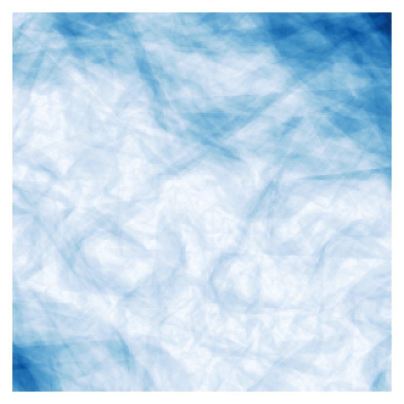
(c) $\lambda=100$

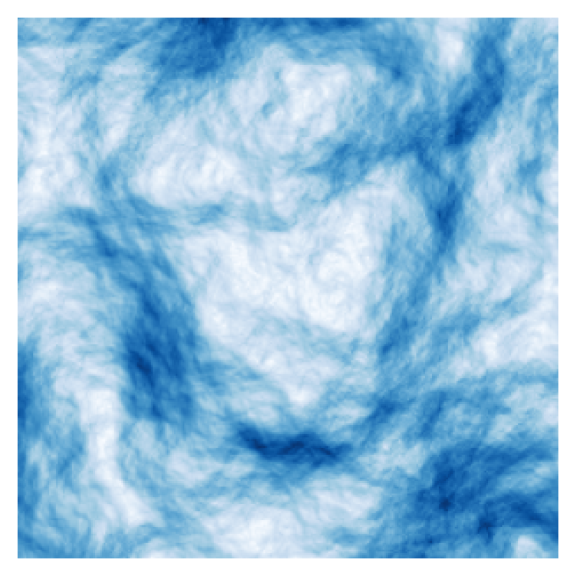
(d) $\lambda=1000$

Figure 1: $\mathbf{P}_{V}$ is Gaussian.

(a) $\lambda=1$

(b) $\lambda=10$

(c) $\lambda=100$

(d) $\lambda=1000$

Figure 2: $\mathbf{P}_{V}$ is symmetric ($\alpha=1.25$)-stable.

7 Conclusion

We have investigated the statistical properties of random ReLU neural networks. We proved that these networks are well-defined non-Gaussian processes in the non-asymptotic regime. We showed that these processes are isotropic and wide-sense self-similar with Hurst exponent $3/2$. Remarkably, the autocovariances of these processes have simple closed-form expressions. Finally, we showed that, under suitable hypotheses, as the expected width tends to infinity, these processes can converge in law not only to Gaussian processes, but also to non-Gaussian processes depending on the law of the weights. These asymptotic results recover the classical observation that wide networks converge to Gaussian processes as well as prove that wide networks can converge to non-Gaussian processes under certain choices of initialization.

Acknowledgments and Disclosure of Funding

This work was supported in part by the Swiss National Science Foundation under Grant 200020_219356 / 1 and in part by the European Research Council (ERC Project FunLearn) under Grant 101020573.

Appendix A Proof of Theorem 9

As preparation before the proof of Theorem 9, we collect and prove some intermediary results. To begin, we shall first prove that $w_{\mathrm{Poi}}$ is a well-defined stochastic process taking values in $\mathcal{S}_{\operatorname{\mathscr{R}}}^{\prime}$. Recall that $w_{\mathrm{Poi}}$ is an impulsive white noise that is realized by a Poisson-type random measure of the form

$$w_{\mathrm{Poi}}=\sum_{k\in\mathbb{Z}}v_{k}\,\delta^{\mathsf{e}}_{({\bm{w}}_{k},b_{k})},$$ (43)

where $v_{k}\overset{\text{i.i.d.}}{\sim}\mathbf{P}_{V}$ for some admissible $\mathbf{P}_{V}$ (in the sense of Definition 5) and the collection of random variables $\mathopen{}\mathclose{{}\left(({\bm{w}}_{k},b_{k})}\right)_{k\in\mathbb{Z}}$ is a (homogeneous) Poisson point process on ${\mathbb{S}^{d-1}\times\mathbb{R}}$ with rate parameter $\lambda>0$. This point process satisfies the following properties.

1. The $({\bm{w}}_{k},b_{k})$ are mutually independent.

2. For any measurable subset $\Pi\subset{\mathbb{S}^{d-1}\times\mathbb{R}}$, if we define the random variable

   $$N_{\Pi}=\lvert\{({\bm{w}}_{k},b_{k})\>\colon\>({\bm{w}}_{k},b_{k})\in\Pi\}\rvert,$$ (44)

   then

   $$\mathbf{P}(N_{\Pi}=n)=\frac{(\lambda\lvert\Pi\rvert)^{n}}{n!}{\mathrm{e}}^{-\lambda\lvert\Pi\rvert},$$ (45)

   where $\lvert\Pi\rvert$ denotes the $d$-dimensional Hausdorff measure of $\Pi$. That is to say, $N_{\Pi}$ is a Poisson random variable with mean $\lambda\lvert\Pi\rvert$.

3. For any measurable subset $B\subset{\mathbb{S}^{d-1}\times\mathbb{R}}$,

   $$\mathbf{P}\mathopen{}\mathclose{{}\left(({\bm{w}}_{k},b_{k})\in B\>|\>({\bm{w}}_{k},b_{k})\in\Pi}\right)=\frac{\lvert B\cap\Pi\rvert}{\lvert\Pi\rvert}.$$ (46)

   That is to say, if a point lies in $\Pi$, then its location will be uniformly distributed on $\Pi$.

Lemma 12

The random measure $w_{\mathrm{Poi}}$ can be viewed as a measurable mapping

$$w_{\mathrm{Poi}}:(\Omega,\mathcal{F},\mathbf{P})\to(\mathcal{S}_{\operatorname{\mathscr{R}}}^{\prime},\operatorname{\mathcal{B}}(\mathcal{S}_{\operatorname{\mathscr{R}}}^{\prime}))$$ (47)

with characteristic functional given by

$$\widehat{\mathbf{P}}_{w_{\mathrm{Poi}}}(\psi)=\exp\mathopen{}\mathclose{{}\left(\lambda\int_{\mathbb{R}}\int_{\mathbb{R}}\int_{\mathbb{S}^{d-1}}\mathopen{}\mathclose{{}\left({\mathrm{e}}^{\mathrm{i}v\psi({\bm{u}},t)}-1}\right)\,\mathrm{d}{\bm{u}}\,\mathrm{d}t\,\mathrm{d}\mathbf{P}_{V}(v)}\right),$$ (48)

where $\mathrm{d}{\bm{u}}$ denotes integration against the surface measure on $\mathbb{S}^{d-1}$.

Proof  Let $\operatorname{\mathcal{D}}(\mathbb{R}^{d})\subset\mathcal{S}(\mathbb{R}^{d})$ denote the space of infinitely differentiable and compactly supported functions on $\mathbb{R}^{d}$. Let $\operatorname{\mathcal{D}}_{\operatorname{\mathscr{R}}}\coloneqq\operatorname{\mathscr{R}}\mathopen{}\mathclose{{}\left(\operatorname{\mathcal{D}}(\mathbb{R}^{d})}\right)$ denote the range of the Radon transform on $\operatorname{\mathcal{D}}(\mathbb{R}^{d})$. We now summarize the properties of $\operatorname{\mathcal{D}}_{\operatorname{\mathscr{R}}}$ that are relevant for our problem (cf., Ludwig, 1966). First, $\operatorname{\mathcal{D}}_{\operatorname{\mathscr{R}}}$ is a closed subspace of $\operatorname{\mathcal{D}}({\mathbb{S}^{d-1}\times\mathbb{R}})$, the nuclear space of infinitely differentiable and compactly supported functions on ${\mathbb{S}^{d-1}\times\mathbb{R}}$ and is therefore nuclear. Furthermore, $\operatorname{\mathcal{D}}_{\operatorname{\mathscr{R}}}$ is dense in $\mathcal{S}_{\operatorname{\mathscr{R}}}$, which implies that $\mathcal{S}_{\operatorname{\mathscr{R}}}^{\prime}$ is continuously embedded in $\operatorname{\mathcal{D}}_{\operatorname{\mathscr{R}}}^{\prime}$. In particular, $\operatorname{\mathcal{D}}_{\operatorname{\mathscr{R}}}$ is the subspace of compactly supported functions in $\mathcal{S}_{\operatorname{\mathscr{R}}}$.

Next, we shall prove that $w_{\mathrm{Poi}}$ can be viewed as a measurable mapping

$$w_{\mathrm{Poi}}:(\Omega,\mathcal{F},\mathbf{P})\to(\operatorname{\mathcal{D}}_{\operatorname{\mathscr{R}}}^{\prime},\operatorname{\mathcal{B}}_{c}(\operatorname{\mathcal{D}}_{\operatorname{\mathscr{R}}}^{\prime}))$$ (49)

by computing its characteristic functional $\widehat{\mathbf{Q}}_{w_{\mathrm{Poi}}}$ on $\operatorname{\mathcal{D}}_{\operatorname{\mathscr{R}}}$. Let $\psi\in\operatorname{\mathcal{D}}_{\operatorname{\mathscr{R}}}$ and let

$$N_{\psi}=\lvert\{({\bm{w}}_{k},b_{k})\>\colon\>({\bm{w}}_{k},b_{k})\in\operatorname{supp}\psi\}\rvert.$$ (50)

We have, by definition, that

$$\langle w_{\mathrm{Poi}},\psi\rangle_{\operatorname{\mathcal{D}}_{\operatorname{\mathscr{R}}}^{\prime}\times\operatorname{\mathcal{D}}_{\operatorname{\mathscr{R}}}}=\sum_{k=1}^{N_{\psi}}v_{k}^{\prime}\psi({\bm{w}}_{k}^{\prime},b_{k}^{\prime}),$$ (51)

where we use an appropriate relabeling of $\{v_{k},{\bm{w}}_{k},b_{k}\>\colon\>({\bm{w}}_{k},b_{k})\in\operatorname{supp}\psi\}$. Therefore,

$$\widehat{\mathbf{Q}}_{w_{\mathrm{Poi}}}(\psi) ={\mathbf{E}}[{\mathrm{e}}^{\mathrm{i}\langle w_{\mathrm{Poi}},\psi\rangle_{\operatorname{\mathcal{D}}_{\operatorname{\mathscr{R}}}^{\prime}\times\operatorname{\mathcal{D}}_{\operatorname{\mathscr{R}}}}}]$$

$$={\mathbf{E}}[{\mathrm{e}}^{\mathrm{i}\sum_{k=1}^{N_{\psi}}v_{k}^{\prime}\psi({\bm{w}}_{k}^{\prime},b_{k}^{\prime})}]$$

$$={\mathbf{E}}\mathopen{}\mathclose{{}\left[{\mathbf{E}}\mathopen{}\mathclose{{}\left[\prod_{k=1}^{N_{\psi}}{\mathrm{e}}^{\mathrm{i}v_{k}^{\prime}\psi({\bm{w}}_{k}^{\prime},b_{k}^{\prime})}\>|\>N_{\psi}}\right]}\right]$$

$$={\mathbf{E}}\mathopen{}\mathclose{{}\left[\prod_{k=1}^{N_{\psi}}{\mathbf{E}}\mathopen{}\mathclose{{}\left[{\mathrm{e}}^{\mathrm{i}v_{k}^{\prime}\psi({\bm{w}}_{k}^{\prime},b_{k}^{\prime})}\>|\>N_{\psi}}\right]}\right]$$ (52)

$$={\mathbf{E}}\mathopen{}\mathclose{{}\left[\prod_{k=1}^{N_{\psi}}{\mathbf{E}}\mathopen{}\mathclose{{}\left[{\mathrm{e}}^{\mathrm{i}v_{k}^{\prime}\psi({\bm{w}}_{k}^{\prime},b_{k}^{\prime})}}\right]}\right]$$

$$={\mathbf{E}}\mathopen{}\mathclose{{}\left[\prod_{k=1}^{N_{\psi}}{\mathbf{E}}\mathopen{}\mathclose{{}\left[{\mathbf{E}}\mathopen{}\mathclose{{}\left[{\mathrm{e}}^{\mathrm{i}v_{k}^{\prime}\psi({\bm{w}}_{k}^{\prime},b_{k}^{\prime})}\>|\>v_{k}}\right]}\right]}\right]$$

$$={\mathbf{E}}\mathopen{}\mathclose{{}\left[\prod_{k=1}^{N_{\psi}}{\mathbf{E}}\mathopen{}\mathclose{{}\left[\frac{1}{\lvert\operatorname{supp}\psi\rvert}\int_{\operatorname{supp}\psi}{\mathrm{e}}^{\mathrm{i}v_{k}^{\prime}\psi({\bm{w}},b)}\,\mathrm{d}({\bm{w}},b)}\right]}\right]$$ (53)

$$={\mathbf{E}}\mathopen{}\mathclose{{}\left[\prod_{k=1}^{N_{\psi}}\frac{1}{\lvert\operatorname{supp}\psi\rvert}\int_{\mathbb{R}}\int_{\operatorname{supp}\psi}{\mathrm{e}}^{\mathrm{i}v\psi({\bm{w}},b)}\,\mathrm{d}({\bm{w}},b)\,\mathrm{d}\mathbf{P}_{V}(v)}\right],$$ (54)

where Eq. 52 holds by the mutual independence of the $({\bm{w}}_{k},b_{k})$ and Eq. 53 holds since the random variables

$$({\bm{w}}_{k}^{\prime},b_{k}^{\prime})\>|\>({\bm{w}}_{k}^{\prime},b_{k}^{\prime})\in\operatorname{supp}\psi$$ (55)

are uniformly distributed on $\operatorname{supp}\psi$. Next, define the auxiliary functional

$$M(\psi)=\int_{\mathbb{R}}\int_{\operatorname{supp}\psi}{\mathrm{e}}^{\mathrm{i}v\psi({\bm{w}},b)}\,\mathrm{d}({\bm{w}},b)\,\mathrm{d}\mathbf{P}_{V}(v).$$ (56)

We have that

$$\widehat{\mathbf{Q}}_{w_{\mathrm{Poi}}}(\psi) ={\mathbf{E}}\mathopen{}\mathclose{{}\left[\prod_{k=1}^{N_{\psi}}\frac{M(\psi)}{\lvert\operatorname{supp}\psi\rvert}}\right]$$

$$={\mathbf{E}}\mathopen{}\mathclose{{}\left[\mathopen{}\mathclose{{}\left(\frac{M(\psi)}{\lvert\operatorname{supp}\psi\rvert}}\right)^{N_{\psi}}}\right]$$

$$=\sum_{n=0}^{\infty}\mathopen{}\mathclose{{}\left(\frac{M(\psi)}{\lvert\operatorname{supp}\psi\rvert}}\right)^{n}\frac{(\lambda\lvert\operatorname{supp}\psi\rvert)^{n}}{n!}{\mathrm{e}}^{-\lambda\lvert\operatorname{supp}\psi\rvert}$$ (57)

$$={\mathrm{e}}^{-\lambda\lvert\operatorname{supp}\psi\rvert}\sum_{n=0}^{\infty}\frac{\mathopen{}\mathclose{{}\left(\lambda M(\psi)}\right)^{n}}{n!}$$

$$={\mathrm{e}}^{-\lambda\lvert\operatorname{supp}\psi\rvert}{\mathrm{e}}^{\lambda M(\psi)}$$ (58)

$$=\exp\mathopen{}\mathclose{{}\left(\lambda(M(\psi)-\lvert\operatorname{supp}\psi\rvert}\right)$$ (59)

$$=\exp\mathopen{}\mathclose{{}\left(\lambda\int_{\mathbb{R}}\int_{{\mathbb{S}^{d-1}\times\mathbb{R}}}\mathopen{}\mathclose{{}\left({\mathrm{e}}^{\mathrm{i}v\psi({\bm{z}})}-1}\right)\,\mathrm{d}{\bm{z}}\,\mathrm{d}\mathbf{P}_{V}(v)}\right),$$ (60)

where Eq. 57 holds since $N_{\psi}$ is a Poisson random variable with mean $\lambda\lvert\operatorname{supp}\psi\rvert$, Eq. 58 holds by the Taylor series expansion of $t\mapsto{\mathrm{e}}^{t}$, Eq. 59 holds since $\lvert\operatorname{supp}\psi\rvert=\int_{\operatorname{supp}\psi}1\,\mathrm{d}{\bm{z}}$, and Eq. 60 holds since ${\bm{z}}\mapsto{\mathrm{e}}^{\mathrm{i}v\psi({\bm{z}})}-1$ vanishes outside $\operatorname{supp}\psi$. At this point, we remark that, since $\mathbf{P}_{V}$ is a Lévy measure (Definition 5), it is well-known that the form of Eq. 60 is continuous, positive definite, and satisfies $\widehat{\mathbf{Q}}_{w_{\mathrm{Poi}}}(0)=1$ (see, e.g., Gelfand and Vilenkin, 1964, Theorem 2, p. 275). This implies that $w_{\mathrm{Poi}}$ is indeed a generalized stochastic process that takes values in $\operatorname{\mathcal{D}}_{\operatorname{\mathscr{R}}}^{\prime}$.

To prove the lemma, it remains to extend the domain of $\widehat{\mathbf{Q}}_{w_{\mathrm{Poi}}}$ to $\mathcal{S}_{\operatorname{\mathscr{R}}}$. To that end, let

$$\widehat{\mathbf{P}}_{w_{\mathrm{Poi}}}(\psi)=\exp\mathopen{}\mathclose{{}\left(\lambda\int_{\mathbb{R}}\int_{{\mathbb{S}^{d-1}\times\mathbb{R}}}\mathopen{}\mathclose{{}\left({\mathrm{e}}^{\mathrm{i}v\psi({\bm{z}})}-1}\right)\,\mathrm{d}{\bm{z}}\,\mathrm{d}\mathbf{P}_{V}(v)}\right),\quad\psi\in\mathcal{S}_{\operatorname{\mathscr{R}}}.$$ (61)

We now invoke an adaption of Fageot et al. (2014, Theorem 3) which investigates impulsive white noise defined on $\mathbb{R}^{d}$ as a special case. Their theorem implies that, thanks to the admissibility conditions on $\mathbf{P}_{V}$ (Definition 5), the probability measures $\mathbf{Q}_{w_{\mathrm{Poi}}}$ and $\mathbf{P}_{w_{\mathrm{Poi}}}$ are compatible on $\operatorname{\mathcal{B}}(\mathcal{S}_{\operatorname{\mathscr{R}}}^{\prime})=\operatorname{\mathcal{B}}_{c}(\mathcal{S}_{\operatorname{\mathscr{R}}}^{\prime})\subset\operatorname{\mathcal{B}}_{c}(\operatorname{\mathcal{D}}_{\operatorname{\mathscr{R}}}^{\prime})$ in the sense that

$$\mathbf{Q}_{w_{\mathrm{Poi}}}(B)=\mathbf{P}_{w_{\mathrm{Poi}}}(B),\quad\text{for all }B\in\operatorname{\mathcal{B}}(\mathcal{S}_{\operatorname{\mathscr{R}}}^{\prime})$$ (62)

and $\mathbf{Q}_{w_{\mathrm{Poi}}}(\operatorname{\mathcal{D}}_{\operatorname{\mathscr{R}}}^{\prime}\setminus\mathcal{S}_{\operatorname{\mathscr{R}}}^{\prime})=0$, which proves the lemma.  

Let $\mathcal{S}_{\Delta}(\mathbb{R}^{d})\coloneqq\Delta\mathopen{}\mathclose{{}\left(\mathcal{S}(\mathbb{R}^{d})}\right)$ denote the range of the Laplacian operator on $\mathcal{S}(\mathbb{R}^{d})$. This is a closed subspace of $\mathcal{S}(\mathbb{R}^{d})$. Observe that its dual $\mathcal{S}_{\Delta}^{\prime}(\mathbb{R}^{d})$ can be identified with the quotient space $\mathcal{S}^{\prime}(\mathbb{R}^{d})/\mathcal{N}_{\Delta}$, where

$$\mathcal{N}_{\Delta}=\{f\in\mathcal{S}^{\prime}(\mathbb{R}^{d})\>\colon\>\Delta f=0\Leftrightarrow\langle f,\phi\rangle_{\mathcal{S}^{\prime}(\mathbb{R}^{d})\times\mathcal{S}(\mathbb{R}^{d})}=0\text{ for all }\phi\in\mathcal{S}_{\Delta}(\mathbb{R}^{d})\}.$$ (63)

is the null space of the Laplacian operator. It is well-known that $\mathcal{N}_{\Delta}$ is infinite-dimensional and that its members are necessary polynomials, the so-called harmonic polynomials. Therefore, the members of $\mathcal{S}_{\Delta}^{\prime}(\mathbb{R}^{d})$ are actually equivalence classes of the form

$$[f]=\{f+h\>\colon\>h\in\mathcal{N}_{\Delta}\}\in\mathcal{S}_{\Delta}^{\prime}(\mathbb{R}^{d}),$$ (64)

where $f\in\mathcal{S}^{\prime}(\mathbb{R}^{d})$. With this notation, we now prove Theorem 9.

Proof [Proof of Theorem 9] Recall that $\operatorname{T}_{\operatorname{ReLU}}=\operatorname{K}\operatorname{\mathscr{R}}\Delta$ and so $\operatorname{T}_{\operatorname{ReLU}}^{*}=\Delta\operatorname{\mathscr{R}}^{*}\operatorname{K}$. Observe that, by Proposition 4,

$$\operatorname{T}_{\operatorname{ReLU}}^{*}:\mathcal{S}_{\operatorname{\mathscr{R}}}\to\mathcal{S}_{\Delta}(\mathbb{R}^{d})$$ (65)

is a continuous bijection, where we equip the closed subspaces $\mathcal{S}_{\operatorname{\mathscr{R}}}\subset\mathcal{S}({\mathbb{S}^{d-1}\times\mathbb{R}})$ and $\mathcal{S}_{\Delta}(\mathbb{R}^{d})\subset\mathcal{S}(\mathbb{R}^{d})$ with the subspace topology from their respective parent Fréchet spaces. By the open mapping theorem for Fréchet spaces (see, e.g., Rudin, 1991, Theorem 2.11), there exists a continuous inverse operator

$$\operatorname{T}_{\operatorname{ReLU}}^{*-}:\mathcal{S}_{\Delta}(\mathbb{R}^{d})\to\mathcal{S}_{\operatorname{\mathscr{R}}}$$ (66)

with the properties that that $\operatorname{T}_{\operatorname{ReLU}}^{*}\operatorname{T}_{\operatorname{ReLU}}^{*-}=\operatorname{Id}$ on $\mathcal{S}_{\Delta}(\mathbb{R}^{d})$ and $\operatorname{T}_{\operatorname{ReLU}}^{*-}\operatorname{T}_{\operatorname{ReLU}}^{*}=\operatorname{Id}$ on $\mathcal{S}_{\operatorname{\mathscr{R}}}$. Therefore, by duality, we have the continuous bijections

$$\operatorname{T}_{\operatorname{ReLU}}:\mathcal{S}_{\Delta}^{\prime}(\mathbb{R}^{d})\to\mathcal{S}_{\operatorname{\mathscr{R}}}$$

$$\operatorname{T}_{\operatorname{ReLU}}^{-}:\mathcal{S}_{\operatorname{\mathscr{R}}}^{\prime}\to\mathcal{S}_{\Delta}^{\prime}(\mathbb{R}^{d}),$$ (67)

where we recall that $\mathcal{S}_{\Delta}^{\prime}(\mathbb{R}^{d})\cong\mathcal{S}^{\prime}(\mathbb{R}^{d})/\mathcal{N}_{\Delta}$.

Next, we note that the operator

$$\operatorname{T}_{\operatorname{ReLU}}^{\dagger\varepsilon*}:\varphi\mapsto\int_{\mathbb{R}^{d}}k^{\varepsilon}_{\bm{x}}(\mkern 1.0mu\cdot\mkern 1.0mu)\varphi({\bm{x}})\,\mathrm{d}{\bm{x}}$$ (68)

specified in Eq. 33 continuously maps $\mathcal{S}_{\Delta}(\mathbb{R}^{d})\to\mathcal{S}_{\operatorname{\mathscr{R}}}$ (cf., Unser, 2023, p. 21). Observe that, by Proposition 7, its extension by duality $\operatorname{T}_{\operatorname{ReLU}}^{\dagger\varepsilon}:\mathcal{S}_{\operatorname{\mathscr{R}}}^{\prime}\to\mathcal{S}_{\Delta}^{\prime}(\mathbb{R}^{d})$ coincides with $\operatorname{T}_{\operatorname{ReLU}}^{-}$. In particular, $\operatorname{T}_{\operatorname{ReLU}}^{\dagger\varepsilon}$ imposes the boundary conditions from Eq. 24 on the affine component of the harmonic polynomials in the equivalence classes in $\mathcal{S}_{\Delta}^{\prime}(\mathbb{R}^{d})$. Said differently, the range space $\operatorname{T}_{\operatorname{ReLU}}^{\dagger\varepsilon}\mathopen{}\mathclose{{}\left(\mathcal{S}_{\operatorname{\mathscr{R}}}^{\prime}}\right)$ is the closed subspace of $\mathcal{S}_{\Delta}^{\prime}(\mathbb{R}^{d})$ whose equivalence class members $[s]\in\mathcal{S}_{\Delta}^{\prime}(\mathbb{R}^{d})$ additionally satisfy

$$\mathopen{}\mathclose{{}\left[(\partial^{\bm{m}}g_{d}^{\varepsilon})*s_{0}}\right]({\bm{0}})=0,\lvert{\bm{m}}\rvert\leq 1$$ (69)

for all $s_{0}\in[s]$. Therefore, we can rewrite the SDE Eq. 34 as

$$s\overset{\mathscr{L}}{=}\operatorname{T}_{\operatorname{ReLU}}^{\dagger\varepsilon}w_{\mathrm{Poi}},$$ (70)

where the equality is understood in $\mathcal{S}_{\Delta}^{\prime}(\mathbb{R}^{d})$, i.e.,

$$\langle s,\phi\rangle_{\mathcal{S}_{\Delta}^{\prime}(\mathbb{R}^{d})\times\mathcal{S}_{\Delta}(\mathbb{R}^{d})}\overset{\mathscr{L}}{=}\langle\operatorname{T}_{\operatorname{ReLU}}^{\dagger\varepsilon}w_{\mathrm{Poi}},\phi\rangle_{\mathcal{S}_{\Delta}^{\prime}(\mathbb{R}^{d})\times\mathcal{S}_{\Delta}(\mathbb{R}^{d})}=\langle w_{\mathrm{Poi}},\operatorname{T}_{\operatorname{ReLU}}^{\dagger\varepsilon*}\phi\rangle_{\mathcal{S}_{\operatorname{\mathscr{R}}}^{\prime}\times\mathcal{S}_{\operatorname{\mathscr{R}}}},$$ (71)

for all $\phi\in\mathcal{S}_{\Delta}(\mathbb{R}^{d})$. The above equality implies that the characteristic functional of any solution $s$ to Eq. 70 (and, subsequently, the original SDE Eq. 34) takes the form

$$\widehat{\mathbf{P}}_{s}(\phi)=\widehat{\mathbf{P}}_{\operatorname{T}_{\operatorname{ReLU}}^{\dagger\varepsilon}w_{\mathrm{Poi}}}(\phi)=\widehat{\mathbf{P}}_{w_{\mathrm{Poi}}}(\operatorname{T}_{\operatorname{ReLU}}^{\dagger\varepsilon*}\phi).$$ (72)

This characteristic functional is well-defined for any $\phi\in\mathcal{S}_{\Delta}(\mathbb{R}^{d})$ since $\operatorname{T}_{\operatorname{ReLU}}^{\dagger\varepsilon*}\phi\in\mathcal{S}_{\operatorname{\mathscr{R}}}$, which ensures that the right-hand side is well-defined by Lemma 12.

Since $s_{\operatorname{ReLU}}^{\varepsilon}\coloneqq\operatorname{T}_{\operatorname{ReLU}}^{\dagger\varepsilon}w_{\mathrm{Poi}}$ via the computation in Eq. 28, we see that $s_{\operatorname{ReLU}}^{\varepsilon}$ is one member in an equivalence class in $\mathcal{S}^{\prime}(\mathbb{R}^{d})/\mathcal{N}_{\Delta}$. In particular, this implies that $s_{\operatorname{ReLU}}\in\mathcal{S}^{\prime}(\mathbb{R}^{d})$ and that the equivalence class $[s_{\operatorname{ReLU}}^{\varepsilon}]=\{s_{\operatorname{ReLU}}^{\varepsilon}+h\>\colon\>h\in\mathcal{N}_{\Delta}\}$ is a well-defined stochastic process that takes values in $\mathcal{S}_{\Delta}^{\prime}(\mathbb{R}^{d})\cong\mathcal{S}^{\prime}(\mathbb{R}^{d})/\mathcal{N}_{\Delta}$ whose characteristic functional on $\mathcal{S}_{\Delta}$ is given by Eq. 72. Equivalently stated, the full set of tempered weak solutions of the SDE Eq. 34 has members that necessarily take the form $s_{\operatorname{ReLU}}^{\varepsilon}+h$, where $h\in\mathcal{N}_{\Delta}$ is a harmonic polynomial of degree $\geq 2$ (since boundary conditions of the SDE, imposed by $\operatorname{T}_{\operatorname{ReLU}}^{\dagger\varepsilon}$, force the affine component of all solutions to be the same). Consequently, from these boundary conditions, we readily see that the only CPwL solution to the SDE is $s_{\operatorname{ReLU}}^{\varepsilon}$.

To complete the proof we need to derive the form of the characteristic functional of $s_{\operatorname{ReLU}}^{\varepsilon}$ on the larger space $\mathcal{S}(\mathbb{R}^{d})\supset\mathcal{S}_{\Delta}(\mathbb{R}^{d})$. For any $\varphi\in\mathcal{S}(\mathbb{R}^{d})$, we have that

$$\langle s_{\operatorname{ReLU}}^{\varepsilon},\varphi\rangle_{\mathcal{S}^{\prime}(\mathbb{R}^{d})\times\mathcal{S}(\mathbb{R}^{d})}\overset{\mathscr{L}}{=}\langle\operatorname{T}_{\operatorname{ReLU}}^{\dagger\varepsilon}w_{\mathrm{Poi}},\varphi\rangle_{\mathcal{S}^{\prime}(\mathbb{R}^{d})\times\mathcal{S}(\mathbb{R}^{d})}$$ (73)

From the expression of the kernel $({\bm{u}},t)\mapsto k^{\varepsilon}_{\bm{x}}({\bm{u}},t)$ in Eq. 26 we see that (i) it is continuous in the variables $({\bm{u}},t)\in{\mathbb{S}^{d-1}\times\mathbb{R}}$ and (ii) it decays faster than any polynomial in the $t$-variable. Therefore, for every $\varphi\in\mathcal{S}(\mathbb{R}^{d})$, the function $\operatorname{T}_{\operatorname{ReLU}}^{\dagger\varepsilon*}\{\varphi\}$ is a continuous function in $({\bm{u}},t)\in{\mathbb{S}^{d-1}\times\mathbb{R}}$ that decays faster than any polynomial in the $t$-variable. In particular, this ensures that, for any $1\leq p\leq\infty$, the map

$$\operatorname{T}_{\operatorname{ReLU}}^{\dagger\varepsilon*}:\mathcal{S}(\mathbb{R}^{d})\to L^{p}({\mathbb{S}^{d-1}\times\mathbb{R}})$$ (74)

is continuous.

The right-hand side of Eq. 73 is, by definition, the integration of $\operatorname{T}_{\operatorname{ReLU}}^{\dagger\varepsilon*}\{\varphi\}$ against the locally finite Radon measure $w_{\mathrm{Poi}}$, i.e., for any $\varphi\in\mathcal{S}(\mathbb{R}^{d})$ we have that

$$\langle s_{\operatorname{ReLU}}^{\varepsilon},\varphi\rangle_{\mathcal{S}^{\prime}(\mathbb{R}^{d})\times\mathcal{S}(\mathbb{R}^{d})} \overset{\mathclap{\mathscr{L}}}{=}\int_{{\mathbb{S}^{d-1}\times\mathbb{R}}}\operatorname{T}_{\operatorname{ReLU}}^{\dagger\varepsilon*}\{\varphi\}\,\mathrm{d}\mathopen{}\mathclose{{}\left(\sum_{k\in\mathbb{Z}}v_{k}\,\delta^{\mathsf{e}}_{({\bm{w}}_{k},b_{k})}}\right)$$

$$=\sum_{k\in\mathbb{Z}}v_{k}\int_{{\mathbb{S}^{d-1}\times\mathbb{R}}}\operatorname{T}_{\operatorname{ReLU}}^{\dagger\varepsilon*}\{\varphi\}\,\mathrm{d}\delta^{\mathsf{e}}_{({\bm{w}}_{k},b_{k})}$$

$$=\sum_{k\in\mathbb{Z}}v_{k}\operatorname{T}_{\operatorname{ReLU}}^{\dagger\varepsilon*}\{\varphi\}({\bm{w}}_{k},b_{k}),$$ (75)

where interchanging of the integral and sum in the second line is well-defined due to the regularity of $\operatorname{T}_{\operatorname{ReLU}}^{\dagger\varepsilon*}\{\varphi\}$ and the third line uses the fact that the range of $\operatorname{T}_{\operatorname{ReLU}}^{\dagger\varepsilon*}$ on $\mathcal{S}(\mathbb{R}^{d})$ is a space of even functions. This proves that

$$\phantom{{}={}}\widehat{\mathbf{P}}_{s_{\operatorname{ReLU}}^{\varepsilon}}(\varphi)$$

$$=\widehat{\mathbf{P}}_{w_{\mathrm{Poi}}}(\operatorname{T}_{\operatorname{ReLU}}^{\dagger\varepsilon*}\varphi)=\exp\mathopen{}\mathclose{{}\left(\lambda\int_{\mathbb{R}}\int_{\mathbb{R}}\int_{\mathbb{S}^{d-1}}\mathopen{}\mathclose{{}\left({\mathrm{e}}^{\mathrm{i}v\operatorname{T}_{\operatorname{ReLU}}^{\dagger\varepsilon*}\{\varphi\}({\bm{u}},t)}-1}\right)\,\mathrm{d}{\bm{u}}\,\mathrm{d}t\,\mathrm{d}\mathbf{P}_{V}(v)}\right),$$ (76)

for all $\varphi\in\mathcal{S}(\mathbb{R}^{d})$, where the last equality comes from Lemma 12. We shall now verify that $\widehat{\mathbf{P}}_{s_{\operatorname{ReLU}}^{\varepsilon}}$ is a valid characteristic functional on $\mathcal{S}(\mathbb{R}^{d})$. This then implies that $s_{\operatorname{ReLU}}^{\varepsilon}:(\Omega,\mathcal{F},\mathbf{P})\to(\mathcal{S}^{\prime}(\mathbb{R}^{d}),\operatorname{\mathcal{B}}(\mathcal{S}^{\prime}(\mathbb{R}^{d}))$ is a measurable mapping and therefore a well-defined stochastic process.

Observe that the second admissibility condition on $\mathbf{P}_{V}$ (Item 2 in Definition 5) states that $\mathbf{P}_{V}$ has a finite absolute moment. This is a sufficient condition to ensure that this characteristic functional Eq. 76 is well-defined for every $\varphi\in\mathcal{S}(\mathbb{R}^{d})$. Indeed, we have that

$$\Psi(\xi)\coloneqq\lambda\int_{\mathbb{R}}\mathopen{}\mathclose{{}\left({\mathrm{e}}^{\mathrm{i}v\xi}-1}\right)\,\mathrm{d}\mathbf{P}_{V}(v)\leq\lambda\,\lvert\xi\rvert\,{\mathbf{E}}[\lvert V\rvert],$$ (77)

where $V\sim\mathbf{P}_{V}$ (cf., Unser et al., 2014, p. 1952). Therefore,

$$\widehat{\mathbf{P}}_{s_{\operatorname{ReLU}}^{\varepsilon}}(\varphi) =\exp\mathopen{}\mathclose{{}\left(\lambda\int_{\mathbb{R}}\int_{\mathbb{R}}\int_{\mathbb{S}^{d-1}}\mathopen{}\mathclose{{}\left({\mathrm{e}}^{\mathrm{i}v\operatorname{T}_{\operatorname{ReLU}}^{\dagger\varepsilon*}\{\varphi\}({\bm{u}},t)}-1}\right)\,\mathrm{d}{\bm{u}}\,\mathrm{d}t\,\mathrm{d}\mathbf{P}_{V}(v)}\right)$$

$$=\exp\mathopen{}\mathclose{{}\left(\int_{{\mathbb{S}^{d-1}\times\mathbb{R}}}\Psi\mathopen{}\mathclose{{}\left(\operatorname{T}_{\operatorname{ReLU}}^{\dagger\varepsilon*}\{\varphi\}}\right)\,\mathrm{d}{\bm{z}}}\right)$$

$$\leq\exp\mathopen{}\mathclose{{}\left(C\,\lVert\operatorname{T}_{\operatorname{ReLU}}^{\dagger\varepsilon*}\{\varphi\}\rVert_{L^{1}}}\right)$$

$$<\infty,$$ (78)

for any $\varphi\in\mathcal{S}(\mathbb{R}^{d})$, where $C=\lambda\,{\mathbf{E}}[\lvert V\rvert]<\infty$, where in the last line we used Eq. 74 with $p=1$. Since $\operatorname{T}_{\operatorname{ReLU}}^{\dagger\varepsilon*}:\mathcal{S}(\mathbb{R}^{d})\to L^{1}({\mathbb{S}^{d-1}\times\mathbb{R}})$ linearly and continuously, Proposition 3.1 of Fageot and Unser (2019) then guarantees that $\widehat{\mathbf{P}}_{s_{\operatorname{ReLU}}}$ is continuous, positive definite, and satisfies $\widehat{\mathbf{P}}_{s_{\operatorname{ReLU}}}(0)=1$. Therefore, the Bochner–Minlos theorem ensures that $\widehat{\mathbf{P}}_{s_{\operatorname{ReLU}}^{\varepsilon}}$ is the characteristic functional of the well-defined stochastic process $s_{\operatorname{ReLU}}^{\varepsilon}$.

By taking $\varepsilon\to 0$, we see that the random neural network $s_{\operatorname{ReLU}}\sim\mathcal{RP}(\lambda;\mathbf{P}_{V})$ is a measurable mapping $(\Omega,\mathcal{F},\mathbf{P})\to(\mathcal{S}^{\prime}(\mathbb{R}^{d}),\operatorname{\mathcal{B}}(\mathcal{S}^{\prime}(\mathbb{R}^{d}))$ whose characteristic functional is

$$\widehat{\mathbf{P}}_{s_{\operatorname{ReLU}}}(\varphi)=\exp\mathopen{}\mathclose{{}\left(\lambda\int_{\mathbb{R}}\int_{\mathbb{R}}\int_{\mathbb{S}^{d-1}}\mathopen{}\mathclose{{}\left({\mathrm{e}}^{\mathrm{i}v\operatorname{T}_{\operatorname{ReLU}}^{\dagger*}\{\varphi\}({\bm{u}},t)}-1}\right)\,\mathrm{d}{\bm{u}}\,\mathrm{d}t\,\mathrm{d}\mathbf{P}_{V}(v)}\right),\quad\varphi\in\mathcal{S}(\mathbb{R}^{d}),$$ (79)

where we observe that this limiting characteristic functional remains to be valid in the sense of the Bochner–Minlos theorem since the property that, for any $1\leq p\leq\infty$, the map

$$\operatorname{T}_{\operatorname{ReLU}}^{\dagger*}:\mathcal{S}(\mathbb{R}^{d})\to L^{p}({\mathbb{S}^{d-1}\times\mathbb{R}})$$ (80)

is continuous, remains to be true since $k_{\bm{x}}=\lim_{\varepsilon\to 0}k^{\varepsilon}_{\bm{x}}$ is compactly supported. Consequently, $s_{\operatorname{ReLU}}$ is the unique CPwL solution to SDE Eq. 36.  

Appendix B Proof of Theorem 10

Proof 

1. Thanks to the moment generating properties of the characteristic functional (Gelfand and Vilenkin, 1964), the mean functional of $s_{\operatorname{ReLU}}$ can be obtained as

   $$\mu_{s_{\operatorname{ReLU}}}(\varphi)={\mathbf{E}}[\langle s_{\operatorname{ReLU}},\varphi\rangle_{\mathcal{S}^{\prime}(\mathbb{R}^{d})\times\mathcal{S}(\mathbb{R}^{d})}]=(-\mathrm{i})\frac{\,\mathrm{d}}{\,\mathrm{d}\xi}\widehat{\mathbf{P}}_{s_{\operatorname{ReLU}}}(\xi\varphi)\Big{\rvert}_{\xi=0},$$ (81)

   where $\varphi\in\mathcal{S}(\mathbb{R}^{d})$. First, observe that the characteristic functional of $s_{\operatorname{ReLU}}$ can be written as

   $$\widehat{\mathbf{P}}_{s_{\operatorname{ReLU}}}(\varphi)=\exp\mathopen{}\mathclose{{}\left(\int_{{\mathbb{S}^{d-1}\times\mathbb{R}}}\Psi\mathopen{}\mathclose{{}\left(\operatorname{T}_{\operatorname{ReLU}}^{\dagger*}\{\varphi\}({\bm{z}})}\right)\,\mathrm{d}{\bm{z}}}\right)$$ (82)

   with $\Psi$ defined as in Eq. 77. Here, note that we have

   $$\Psi^{\prime}(x)=\mathrm{i}\lambda\int_{\mathbb{R}}v{\mathrm{e}}^{\mathrm{i}vx}\,\mathrm{d}\mathbf{P}_{V}(v).$$ (83)

   Let us denote $h({\bm{z}})=\operatorname{T}_{\operatorname{ReLU}}^{\dagger*}\{\varphi\}({\bm{z}})$. By applying the chain rule, we can write

   $$\dfrac{\mathrm{d}{}}{\mathrm{d}{\xi}}\widehat{\mathbf{P}}_{s_{\operatorname{ReLU}}}(\xi\varphi)=\exp\mathopen{}\mathclose{{}\left(\int_{\mathbb{R}\times\mathbb{S}^{d-1}}\Psi\mathopen{}\mathclose{{}\left(\xi h({\bm{z}})}\right)\,\mathrm{d}{\bm{z}}}\right)\cdot\int_{\mathbb{R}\times\mathbb{S}^{d-1}}\Psi^{\prime}\mathopen{}\mathclose{{}\left(\xi h({\bm{z}})}\right)h({\bm{z}})\,\mathrm{d}{\bm{z}}.$$ (84)

   On setting $\xi=0$, we get

   $$\dfrac{\mathrm{d}{}}{\mathrm{d}{\xi}}\widehat{\mathbf{P}}_{s_{\operatorname{ReLU}}}(\xi\varphi)\Big{\rvert}_{\xi=0}=\Psi^{\prime}(0)\int_{\mathbb{R}\times\mathbb{S}^{d-1}}h({\bm{z}})\,\mathrm{d}{\bm{z}}$$ (85)

   as $\Psi(0)=0$. Therefore, the mean functional is

   $$\mu_{s_{\operatorname{ReLU}}}(\varphi) =(-\mathrm{i})\frac{\,\mathrm{d}}{\,\mathrm{d}\xi}\widehat{\mathbf{P}}_{s_{\operatorname{ReLU}}}(\xi\varphi)\Big{\rvert}_{\xi=0}$$

   $$=\lambda{\mathbf{E}}[V]\int_{{\mathbb{S}^{d-1}\times\mathbb{R}}}\operatorname{T}_{\operatorname{ReLU}}^{\dagger*}\{\varphi\}({\bm{z}})\,\mathrm{d}{\bm{z}}$$

   $$=\lambda{\mathbf{E}}[V]\int_{\mathbb{R}^{d}}\int_{\mathbb{R}}\int_{\mathbb{S}^{d-1}}k_{{\bm{x}}}({\bm{u}},t)\varphi({\bm{x}})\,\mathrm{d}{\bm{u}}\,\mathrm{d}t\,\mathrm{d}{\bm{x}}.$$ (86)

   Next, we establish a link between the mean functional of $s_{\operatorname{ReLU}}$ and the quantity ${\mathbf{E}}[s_{\operatorname{ReLU}}({\bm{x}})]$. Since $s_{\operatorname{ReLU}}$ has a pointwise interpretation, we have

   $$\langle s_{\operatorname{ReLU}},\varphi\rangle_{\mathcal{S}^{\prime}(\mathbb{R}^{d})\times\mathcal{S}(\mathbb{R}^{d})}=\int_{\mathbb{R}^{d}}s_{\operatorname{ReLU}}({\bm{x}})\varphi({\bm{x}})\,\mathrm{d}{\bm{x}}.$$ (87)

   Consequently, the mean functional can also be computed as

   $$\mu_{s_{\operatorname{ReLU}}}(\varphi) ={\mathbf{E}}[\langle s_{\operatorname{ReLU}},\varphi\rangle_{\mathcal{S}^{\prime}(\mathbb{R}^{d})\times\mathcal{S}(\mathbb{R}^{d})}]={\mathbf{E}}\mathopen{}\mathclose{{}\left[\int_{\mathbb{R}^{d}}s_{\operatorname{ReLU}}({\bm{x}})\varphi({\bm{x}})\,\mathrm{d}{\bm{x}}}\right]$$

   $$=\int_{\mathbb{R}^{d}}{\mathbf{E}}[s_{\operatorname{ReLU}}({\bm{x}})]\varphi({\bm{x}})\,\mathrm{d}{\bm{x}},$$ (88)

   where exchanging the expectation and the integral is justified by the Fubini–Tonelli theorem since the integrand in Eq. 86 is absolutely integrable by Eq. 80 with $p=1$. On comparing Eq. 88 with Eq. 86, we see that

   $${\mathbf{E}}[s_{\operatorname{ReLU}}({\bm{x}})]=\lambda{\mathbf{E}}[V]\int_{\mathbb{R}}\int_{\mathbb{S}^{d-1}}k_{{\bm{x}}}({\bm{u}},t)\,\mathrm{d}{\bm{u}}\,\mathrm{d}t.$$ (89)

2. The covariance functional of $s_{\operatorname{ReLU}}$ is given by

   $$\phantom{{}={}}\Sigma_{s_{\operatorname{ReLU}}}(\varphi_{1},\varphi_{2})$$

   $$={\mathbf{E}}\Big{[}\mathopen{}\mathclose{{}\left(\langle s_{\operatorname{ReLU}},\varphi_{1}\rangle_{\mathcal{S}^{\prime}(\mathbb{R}^{d})\times\mathcal{S}(\mathbb{R}^{d})}-\mu_{s_{\operatorname{ReLU}}}(\varphi_{1})}\right)\mathopen{}\mathclose{{}\left(\langle s_{\operatorname{ReLU}},\varphi_{2}\rangle_{\mathcal{S}^{\prime}(\mathbb{R}^{d})\times\mathcal{S}(\mathbb{R}^{d})}-\mu_{s_{\operatorname{ReLU}}}(\varphi_{2})}\right)\Big{]}$$

   $$=\mathcal{R}_{s_{\operatorname{ReLU}}}(\varphi_{1},\varphi_{2})-\mu_{s_{\operatorname{ReLU}}}(\varphi_{1})\mu_{s_{\operatorname{ReLU}}}(\varphi_{2}),$$ (90)

   where $\varphi_{1},\varphi_{2}\in\mathcal{S}(\mathbb{R}^{d})$ and

   $$\mathcal{R}_{s_{\operatorname{ReLU}}}(\varphi_{1},\varphi_{2})={\mathbf{E}}\mathopen{}\mathclose{{}\left[\langle s_{\operatorname{ReLU}},\varphi_{1}\rangle_{\mathcal{S}^{\prime}(\mathbb{R}^{d})\times\mathcal{S}(\mathbb{R}^{d})}\ \langle s_{\operatorname{ReLU}},\varphi_{2}\rangle_{\mathcal{S}^{\prime}(\mathbb{R}^{d})\times\mathcal{S}(\mathbb{R}^{d})}}\right]$$ (91)

   is the correlation functional of $s_{\operatorname{ReLU}}$. This quantity can be computed from its characteristic functional (cf., Gelfand and Vilenkin, 1964) as

   $$\mathcal{R}_{s_{\operatorname{ReLU}}}(\varphi_{1},\varphi_{2})=-\frac{\mathrm{d}^{2}}{\mathrm{d}\xi_{1}\mathrm{d}\xi_{2}}\widehat{\mathbf{P}}_{s_{\operatorname{ReLU}}}(\xi_{1}\varphi_{1}+\xi_{2}\varphi_{2})\Big{\rvert}_{\xi_{1}=0,\xi_{2}=0}.$$ (92)

   Let us first define the quantity $f(\xi_{1},\xi_{2})$ as

   $$f(\xi_{1},\xi_{2}) =\int_{{\mathbb{S}^{d-1}\times\mathbb{R}}}\Psi\mathopen{}\mathclose{{}\left(\operatorname{T}_{\operatorname{ReLU}}^{\dagger*}\{\xi_{1}\varphi_{1}+\xi_{2}\varphi_{2}\}({\bm{z}})}\right)\,\mathrm{d}{\bm{z}}$$

   $$=\int_{{\mathbb{S}^{d-1}\times\mathbb{R}}}\Psi\mathopen{}\mathclose{{}\left(\xi_{1}\operatorname{T}_{\operatorname{ReLU}}^{\dagger*}\{\varphi_{1}\}({\bm{z}})+\xi_{2}\operatorname{T}_{\operatorname{ReLU}}^{\dagger*}\{\varphi_{2}\}({\bm{z}})}\right)\,\mathrm{d}{\bm{z}}.$$ (93)

   Further, let us denote $h_{1}({\bm{z}})=\operatorname{T}_{\operatorname{ReLU}}^{\dagger*}\{\varphi_{1}\}({\bm{z}})$ and $h_{2}({\bm{z}})=\operatorname{T}_{\operatorname{ReLU}}^{\dagger*}\{\varphi_{2}\}({\bm{z}})$. By applying the chain rule twice, we write

   $$\frac{\mathrm{d}^{2}}{\mathrm{d}\xi_{1}\mathrm{d}\xi_{2}}\widehat{\mathbf{P}}_{s_{\operatorname{ReLU}}}(\xi_{1}\varphi_{1} +\xi_{2}\varphi_{2})$$

   $$=\exp(f(\xi_{1},\xi_{2}))\mathopen{}\mathclose{{}\left(\frac{\mathrm{d}^{2}}{\mathrm{d}\xi_{1}\mathrm{d}\xi_{2}}f(\xi_{1},\xi_{2})+\frac{\mathrm{d}}{\mathrm{d}\xi_{1}}f(\xi_{1},\xi_{2})\frac{\mathrm{d}}{\mathrm{d}\xi_{2}}f(\xi_{1},\xi_{2})}\right),$$ (94)

   where

   $$\frac{\mathrm{d}}{\mathrm{d}\xi_{k}}f(\xi_{1},\xi_{2})=\int_{{\mathbb{S}^{d-1}\times\mathbb{R}}}\Psi^{\prime}\mathopen{}\mathclose{{}\left(\xi_{1}h_{1}({\bm{z}})+\xi_{2}h_{2}({\bm{z}})}\right)h_{k}({\bm{z}})\,\mathrm{d}{\bm{z}}$$ (95)

   and

   $$\frac{\mathrm{d}^{2}}{\mathrm{d}\xi_{1}\mathrm{d}\xi_{2}}f(\xi_{1},\xi_{2})=\int_{{\mathbb{S}^{d-1}\times\mathbb{R}}}\Psi^{\prime\prime}\mathopen{}\mathclose{{}\left(\xi_{1}h_{1}({\bm{z}})+\xi_{2}h_{2}({\bm{z}})}\right)h_{1}({\bm{z}})h_{2}({\bm{z}})\,\mathrm{d}{\bm{z}}.$$ (96)

   On setting $\xi_{1}=0$ and $\xi_{2}=0$, we get

   $$\frac{\mathrm{d}^{2}}{\mathrm{d}\xi_{1}\mathrm{d}\xi_{2}}\widehat{\mathbf{P}}_{s_{\operatorname{ReLU}}}(\xi_{1}\varphi_{1}+\xi_{2}\varphi_{2}) \Big{\rvert}_{\xi_{1}=0,\xi_{2}=0}=\ \Psi^{\prime\prime}(0)\int_{{\mathbb{S}^{d-1}\times\mathbb{R}}}h_{1}({\bm{z}})h_{2}({\bm{z}})\,\mathrm{d}{\bm{z}}$$

   $$+\mathopen{}\mathclose{{}\left(\Psi^{\prime}(0)\int_{{\mathbb{S}^{d-1}\times\mathbb{R}}}h_{1}({\bm{z}})\mathrm{d}{\bm{z}}}\right)\mathopen{}\mathclose{{}\left(\Psi^{\prime}(0)\int_{{\mathbb{S}^{d-1}\times\mathbb{R}}}h_{2}({\bm{z}})\,\mathrm{d}{\bm{z}}}\right).$$ (97)

   Note that we have

   $$\Psi^{\prime\prime}(x)=-\lambda\int_{\mathbb{R}}v^{2}{\mathrm{e}}^{\mathrm{i}vx}\,\mathrm{d}\mathbf{P}_{V}(v).$$ (98)

   Thus, the correlation functional is of the form

   $$\mathcal{R}_{s_{\operatorname{ReLU}}}(\varphi_{1},\varphi_{2}) =-\frac{\mathrm{d}^{2}}{\mathrm{d}\xi_{1}\mathrm{d}\xi_{2}}\widehat{\mathbf{P}}_{s_{\operatorname{ReLU}}}(\xi_{1}\varphi_{1}+\xi_{2}\varphi_{2})\Big{\rvert}_{\xi_{1}=0,\xi_{2}=0}$$

   $$=\lambda{\mathbf{E}}[V^{2}]\mathopen{}\mathclose{{}\left(\int_{{\mathbb{S}^{d-1}\times\mathbb{R}}}\operatorname{T}_{\operatorname{ReLU}}^{\dagger*}\{\varphi_{1}\}({\bm{z}})\operatorname{T}_{\operatorname{ReLU}}^{\dagger*}\{\varphi_{2}\}({\bm{z}})\,\mathrm{d}{\bm{z}}}\right)$$

   $$\ \ \ \ +\mu_{s_{\operatorname{ReLU}}}(\varphi_{1})\mu_{s_{\operatorname{ReLU}}}(\varphi_{2}).$$ (99)

   Consequently, the covariance functional is given by

   $$\phantom{{}={}}\Sigma_{s_{\operatorname{ReLU}}}(\varphi_{1},\varphi_{2})$$

   $$=\lambda{\mathbf{E}}[V^{2}]\int_{{\mathbb{S}^{d-1}\times\mathbb{R}}}\operatorname{T}_{\operatorname{ReLU}}^{\dagger*}\{\varphi_{1}\}({\bm{z}})\operatorname{T}_{\operatorname{ReLU}}^{\dagger*}\{\varphi_{2}\}({\bm{z}})\,\mathrm{d}{\bm{z}}$$

   $$=\lambda{\mathbf{E}}[V^{2}]\int_{\mathbb{R}^{d}}\int_{\mathbb{R}^{d}}\int_{\mathbb{R}}\int_{\mathbb{S}^{d-1}}k_{{\bm{x}}}({\bm{u}},t)k_{{\bm{y}}}({\bm{u}},t)\varphi_{1}({\bm{x}})\varphi_{2}({\bm{y}})\,\mathrm{d}{\bm{u}}\,\mathrm{d}t\,\mathrm{d}{\bm{x}}\,\mathrm{d}{\bm{y}}.$$ (100)

   Next, we derive the connection between the covariance functional of $s_{\operatorname{ReLU}}$ and the autocovariance ${\mathbf{E}}[(s_{\operatorname{ReLU}}({\bm{x}})-{\mathbf{E}}[s_{\operatorname{ReLU}}({\bm{x}})])(s_{\operatorname{ReLU}}({\bm{y}})-{\mathbf{E}}[s_{\operatorname{ReLU}}({\bm{y}})])]$. Since $s_{\operatorname{ReLU}}$ has a pointwise interpretation, the covariance functional can also be computed as

   $$\phantom{{}={}}\Sigma_{s_{\operatorname{ReLU}}}(\varphi_{1},\varphi_{2})$$

   $$={\mathbf{E}}\Big{[}\mathopen{}\mathclose{{}\left(\langle s_{\operatorname{ReLU}},\varphi_{1}\rangle_{\mathcal{S}^{\prime}(\mathbb{R}^{d})\times\mathcal{S}(\mathbb{R}^{d})}-\mu_{s_{\operatorname{ReLU}}}(\varphi_{1})}\right)\mathopen{}\mathclose{{}\left(\langle s_{\operatorname{ReLU}},\varphi_{2}\rangle_{\mathcal{S}^{\prime}(\mathbb{R}^{d})\times\mathcal{S}(\mathbb{R}^{d})}-\mu_{s_{\operatorname{ReLU}}}(\varphi_{2})}\right)\Big{]}$$

   $$={\mathbf{E}}\mathopen{}\mathclose{{}\left[\mathopen{}\mathclose{{}\left(\int_{\mathbb{R}^{d}}\mathopen{}\mathclose{{}\left(s_{\operatorname{ReLU}}({\bm{x}})-{\mathbf{E}}[s_{\operatorname{ReLU}}({\bm{x}})]}\right)\varphi_{1}({\bm{x}})\,\mathrm{d}{\bm{x}}}\right)\mathopen{}\mathclose{{}\left(\int_{\mathbb{R}^{d}}\mathopen{}\mathclose{{}\left(s_{\operatorname{ReLU}}({\bm{y}})-{\mathbf{E}}[s_{\operatorname{ReLU}}({\bm{y}})]}\right)\varphi_{2}({\bm{y}})\,\mathrm{d}{\bm{y}}}\right)}\right]$$

   $$=\int_{\mathbb{R}^{d}}\int_{\mathbb{R}^{d}}{\mathbf{E}}[(s_{\operatorname{ReLU}}({\bm{x}})-{\mathbf{E}}[s_{\operatorname{ReLU}}({\bm{x}})])(s_{\operatorname{ReLU}}({\bm{y}})-{\mathbf{E}}[s_{\operatorname{ReLU}}({\bm{y}})])]\varphi_{1}({\bm{x}})\varphi_{2}({\bm{y}})\,\mathrm{d}{\bm{x}}\,\mathrm{d}{\bm{y}},$$ (101)

   where exchanging the expectation and the integral is justified by the Fubini–Tonelli theorem since the integrand in Eq. 100 is absolutely integrable from Eq. 80 with $p=2$. If we compare Eq. 101 with Eq. 100, we see that

   $$C_{s_{\operatorname{ReLU}}}({\bm{x}},{\bm{y}}) ={\mathbf{E}}[(s_{\operatorname{ReLU}}({\bm{x}})-{\mathbf{E}}[s_{\operatorname{ReLU}}({\bm{x}})])(s_{\operatorname{ReLU}}({\bm{y}})-{\mathbf{E}}[s_{\operatorname{ReLU}}({\bm{y}})])]$$

   $$=\lambda{\mathbf{E}}[V^{2}]\int_{\mathbb{R}}\int_{\mathbb{S}^{d-1}}k_{{\bm{x}}}({\bm{u}},t)k_{{\bm{y}}}({\bm{u}},t)\,\mathrm{d}{\bm{u}}\,\mathrm{d}t.$$ (102)

   To simplify the double integral in Eq. 102, we first observe that, by definition,

   $$({\bm{x}},{\bm{y}})\mapsto\int_{\mathbb{R}}\int_{\mathbb{S}^{d-1}}k_{{\bm{x}}}({\bm{u}},t)k_{{\bm{y}}}({\bm{u}},t)\,\mathrm{d}{\bm{u}}\,\mathrm{d}t,\quad({\bm{x}},{\bm{y}})\in\mathbb{R}^{d}\times\mathbb{R}^{d},$$ (103)

   is the (Schwartz) kernel of the operator $\operatorname{T}_{\operatorname{ReLU}}^{\dagger}\operatorname{T}_{\operatorname{ReLU}}^{\dagger*}$. Next, we note that the right-inverse operator can be equivalently specified as the composition of operators $\operatorname{T}_{\operatorname{ReLU}}^{\dagger}=(\operatorname{Id}-\operatorname{P})\Delta^{-1}\operatorname{\mathscr{R}}^{*}$ (cf. Unser, 2023, Equation (57)), where $\Delta^{-1}$ is the Riesz potential of order $2$, i.e., it is the Fourier multiplier

   $$\leavevmode\hbox{\set@color\hskip 15.78825pt\leavevmode\hbox{\set@color$(-\Delta)^{-\frac{\gamma}{2}}f$}\raisebox{2.49445pt}{\leavevmode\hbox{\set@color$\leavevmode\hbox{\set@color\raisebox{0.0pt}{\leavevmode\resizebox{0.10333pt}{10.33327pt}{\hbox{\raisebox{0.0pt}{$\mathchoice{\raisebox{0.0pt}{\leavevmode\resizebox{0.0pt}{614.295pt}{\hbox{\raisebox{0.0pt}{$\displaystyle\mathchoice{\raisebox{0.0pt}{\leavevmode\resizebox{0.0pt}{614.295pt}{\hbox{\raisebox{0.0pt}{$\displaystyle\kern 0.1pt\mathchar 866\relax\kern 0.1pt$}}}}}{\raisebox{0.0pt}{\leavevmode\resizebox{0.0pt}{614.295pt}{\hbox{\raisebox{0.0pt}{$\textstyle\kern 0.1pt\mathchar 866\relax\kern 0.1pt$}}}}}{\raisebox{0.0pt}{\leavevmode\resizebox{0.0pt}{614.295pt}{\hbox{\raisebox{0.0pt}{$\scriptstyle\kern 0.1pt\mathchar 866\relax\kern 0.1pt$}}}}}{\raisebox{0.0pt}{\leavevmode\resizebox{0.0pt}{614.295pt}{\hbox{\raisebox{0.0pt}{$\scriptscriptstyle\kern 0.1pt\mathchar 866\relax\kern 0.1pt$}}}}}$}}}}}{\raisebox{0.0pt}{\leavevmode\resizebox{0.0pt}{614.295pt}{\hbox{\raisebox{0.0pt}{$\textstyle\mathchoice{\raisebox{0.0pt}{\leavevmode\resizebox{0.0pt}{614.295pt}{\hbox{\raisebox{0.0pt}{$\displaystyle\kern 0.1pt\mathchar 866\relax\kern 0.1pt$}}}}}{\raisebox{0.0pt}{\leavevmode\resizebox{0.0pt}{614.295pt}{\hbox{\raisebox{0.0pt}{$\textstyle\kern 0.1pt\mathchar 866\relax\kern 0.1pt$}}}}}{\raisebox{0.0pt}{\leavevmode\resizebox{0.0pt}{614.295pt}{\hbox{\raisebox{0.0pt}{$\scriptstyle\kern 0.1pt\mathchar 866\relax\kern 0.1pt$}}}}}{\raisebox{0.0pt}{\leavevmode\resizebox{0.0pt}{614.295pt}{\hbox{\raisebox{0.0pt}{$\scriptscriptstyle\kern 0.1pt\mathchar 866\relax\kern 0.1pt$}}}}}$}}}}}{\raisebox{0.0pt}{\leavevmode\resizebox{0.0pt}{614.295pt}{\hbox{\raisebox{0.0pt}{$\scriptstyle\mathchoice{\raisebox{0.0pt}{\leavevmode\resizebox{0.0pt}{614.295pt}{\hbox{\raisebox{0.0pt}{$\displaystyle\kern 0.1pt\mathchar 866\relax\kern 0.1pt$}}}}}{\raisebox{0.0pt}{\leavevmode\resizebox{0.0pt}{614.295pt}{\hbox{\raisebox{0.0pt}{$\textstyle\kern 0.1pt\mathchar 866\relax\kern 0.1pt$}}}}}{\raisebox{0.0pt}{\leavevmode\resizebox{0.0pt}{614.295pt}{\hbox{\raisebox{0.0pt}{$\scriptstyle\kern 0.1pt\mathchar 866\relax\kern 0.1pt$}}}}}{\raisebox{0.0pt}{\leavevmode\resizebox{0.0pt}{614.295pt}{\hbox{\raisebox{0.0pt}{$\scriptscriptstyle\kern 0.1pt\mathchar 866\relax\kern 0.1pt$}}}}}$}}}}}{\raisebox{0.0pt}{\leavevmode\resizebox{0.0pt}{614.295pt}{\hbox{\raisebox{0.0pt}{$\scriptscriptstyle\mathchoice{\raisebox{0.0pt}{\leavevmode\resizebox{0.0pt}{614.295pt}{\hbox{\raisebox{0.0pt}{$\displaystyle\kern 0.1pt\mathchar 866\relax\kern 0.1pt$}}}}}{\raisebox{0.0pt}{\leavevmode\resizebox{0.0pt}{614.295pt}{\hbox{\raisebox{0.0pt}{$\textstyle\kern 0.1pt\mathchar 866\relax\kern 0.1pt$}}}}}{\raisebox{0.0pt}{\leavevmode\resizebox{0.0pt}{614.295pt}{\hbox{\raisebox{0.0pt}{$\scriptstyle\kern 0.1pt\mathchar 866\relax\kern 0.1pt$}}}}}{\raisebox{0.0pt}{\leavevmode\resizebox{0.0pt}{614.295pt}{\hbox{\raisebox{0.0pt}{$\scriptscriptstyle\kern 0.1pt\mathchar 866\relax\kern 0.1pt$}}}}}$}}}}}$}}}}}$}}\hskip 15.78825pt}({\bm{\omega}})=\lVert{\bm{\omega}}\rVert_{2}^{-\gamma}\,\widehat{f}({\bm{\omega}}),\quad{\bm{\omega}}\in\mathbb{R}^{d},$$ (104)

   with $\gamma=2$, and $\operatorname{P}$ is the projection onto the space of affine functions adapted to the boundary conditions of the SDE Eq. 36. Concretely,

   $$\operatorname{P}\{f\}=\sum_{n=0}^{d}\langle\phi_{n},f\rangle p_{n},$$ (105)

   where $p_{0}({\bm{x}})=1$ and $p_{n}({\bm{x}})=x_{n}$, $n=1,\ldots,d$ is a basis for the space of affine function on $\mathbb{R}^{d}$ and $\phi_{0}=\delta$ (Dirac distribution) and $\phi_{n}=-\delta_{n}^{\prime}\coloneqq-\partial_{x_{n}}\delta$, $n=1,\ldots,d$, is the linear functional that evaluates the partial derivative in the $n$th component at ${\bm{0}}$, i.e., $\langle\phi_{n},f\rangle=\partial_{x_{n}}f({\bm{0}})$, $n=1,\ldots,d$. Consequently, the adjoint projector is given by

   $$\operatorname{P}^{*}\{f\}=\sum_{n=0}^{d}\langle p_{n},f\rangle\phi_{n}.$$ (106)

   With this notation, we have that

   $$\operatorname{T}_{\operatorname{ReLU}}^{\dagger}\operatorname{T}_{\operatorname{ReLU}}^{\dagger*} =(\operatorname{Id}-\operatorname{P})\Delta^{-1}\operatorname{\mathscr{R}}^{*}\operatorname{\mathscr{R}}\Delta^{-1}(\operatorname{Id}-\operatorname{P}^{*})$$

   $$=(\operatorname{Id}-\operatorname{P})\Delta^{-1}(-\Delta)^{-\frac{d-1}{2}}\Delta^{-1}(\operatorname{Id}-\operatorname{P}^{*})$$

   $$=(\operatorname{Id}-\operatorname{P})(-\Delta)^{-\frac{d+3}{2}}(\operatorname{Id}-\operatorname{P}^{*}),$$ (107)

   where the second line follows from Proposition 4. The (Schwartz) kernel of the operator (generalized impulse response) can be identified with $({\bm{x}},{\bm{y}})\mapsto\operatorname{T}_{\operatorname{ReLU}}^{\dagger}\operatorname{T}_{\operatorname{ReLU}}^{\dagger*}\{\delta(\mkern 1.0mu\cdot\mkern 1.0mu-{\bm{y}})\}({\bm{x}})$. We have that

   $$(\operatorname{Id}-\operatorname{P}^{*})\{\delta(\mkern 1.0mu\cdot\mkern 1.0mu-{\bm{y}})\}=\delta(\mkern 1.0mu\cdot\mkern 1.0mu-{\bm{y}})-\sum_{k=0}^{d}\langle p_{k},\delta(\mkern 1.0mu\cdot\mkern 1.0mu-{\bm{y}})\rangle\phi_{n}=\delta(\mkern 1.0mu\cdot\mkern 1.0mu-{\bm{y}})-\delta+\sum_{n=1}^{d}y_{1}\delta_{n}^{\prime},$$ (108)

   where we used the property that the shifted Dirac distribution is the sampling functional. Next,

   $$(-\Delta)^{-\frac{d+3}{2}}(\operatorname{Id}-\operatorname{P}^{*})\{\delta(\mkern 1.0mu\cdot\mkern 1.0mu-{\bm{y}})\}({\bm{x}}) =A\mathopen{}\mathclose{{}\left(\lVert{\bm{x}}-{\bm{y}}\rVert_{2}^{3}-\lVert{\bm{x}}\rVert_{2}^{3}+\sum_{n=1}^{d}y_{1}(3x_{n}\lVert{\bm{x}}\rVert_{2})}\right)$$

   $$=A\mathopen{}\mathclose{{}\left(\lVert{\bm{x}}-{\bm{y}}\rVert_{2}^{3}-\lVert{\bm{x}}\rVert_{2}^{3}+3{\bm{x}}^{\mathsf{T}}{\bm{y}}\lVert{\bm{x}}\rVert_{2}}\right),$$ (109)

   where $A=\frac{\Gamma(-3/2)}{2^{d+3}\pi^{d/2}\Gamma((d+3)/2)}$ and we used the fact that ${\bm{x}}\mapsto A\lVert{\bm{x}}\rVert_{2}^{3}$ is the radially symmetric Green’s function of $(-\Delta)^{\frac{d+3}{2}}$ (Gelfand and Shilov, 1964). Finally,

   $$\phantom{{}={}}(\operatorname{Id}-\operatorname{P})(-\Delta)^{-\frac{d+3}{2}}(\operatorname{Id}-\operatorname{P}^{*})\{\delta(\mkern 1.0mu\cdot\mkern 1.0mu-{\bm{y}})\}({\bm{x}})$$

   $$=A\mathopen{}\mathclose{{}\left(\lVert{\bm{x}}-{\bm{y}}\rVert_{2}^{3}-\lVert{\bm{x}}\rVert_{2}^{3}+3{\bm{x}}^{\mathsf{T}}{\bm{y}}\lVert{\bm{x}}\rVert_{2}}\right)-A\mathopen{}\mathclose{{}\left(\lVert{\bm{y}}\rVert_{2}^{3}-\sum_{n=1}^{d}3y_{n}\lVert{\bm{y}}\rVert_{2}x_{n}}\right)$$

   $$=A\mathopen{}\mathclose{{}\left(\lVert{\bm{x}}-{\bm{y}}\rVert_{2}^{3}-\lVert{\bm{x}}\rVert_{2}^{3}-\lVert{\bm{y}}\rVert_{2}^{3}+3{\bm{x}}^{\mathsf{T}}{\bm{y}}\mathopen{}\mathclose{{}\left(\lVert{\bm{x}}\rVert_{2}+\lVert{\bm{y}}\rVert_{2}}\right)}\right).$$ (110)

   Putting everything together, we find that the autocovariance takes the form

   $$C_{s_{\operatorname{ReLU}}}({\bm{x}},{\bm{y}})=\lambda A{\mathbf{E}}[V^{2}]\mathopen{}\mathclose{{}\left(\lVert{\bm{x}}-{\bm{y}}\rVert_{2}^{3}-\lVert{\bm{x}}\rVert_{2}^{3}-\lVert{\bm{y}}\rVert_{2}^{3}+3{\bm{x}}^{\mathsf{T}}{\bm{y}}\mathopen{}\mathclose{{}\left(\lVert{\bm{x}}\rVert_{2}+\lVert{\bm{y}}\rVert_{2}}\right)}\right).$$ (111)

3. In order to show that $s_{\operatorname{ReLU}}$ is isotropic, we will show that its characteristic functional satisfies

   $$\widehat{\mathbf{P}}_{s_{\operatorname{ReLU}}}(\varphi)=\widehat{\mathbf{P}}_{s_{\operatorname{ReLU}}}\mathopen{}\mathclose{{}\left(\varphi\mathopen{}\mathclose{{}\left(\mathbf{U}\cdot}\right)}\right)$$ (112)

   for any $\varphi\in\mathcal{S}(\mathbb{R}^{d})$ and any $(d\times d)$ rotation matrix $\mathbf{U}$. First, we note that the kernel of $\operatorname{T}_{\operatorname{ReLU}}^{\dagger}$ can be written as

   $$k_{\bm{x}}({\bm{u}},t) =\operatorname{ReLU}({\bm{u}}^{\mathsf{T}}{\bm{x}}-t)-\frac{({\bm{u}}^{\mathsf{T}}{\bm{x}}-t)}{2}-\frac{\lvert t\rvert}{2}+({\bm{u}}^{\mathsf{T}}{\bm{x}})\frac{\operatorname{sgn}(t)}{2}$$

   $$=\operatorname{ReLU}({\bm{u}}^{\mathsf{T}}{\bm{x}}-t)+({\bm{u}}^{\mathsf{T}}{\bm{x}})h_{1}(t)+h_{2}(t),$$ (113)

   where $h_{1}(t)=\frac{\operatorname{sgn}(t)-1}{2}$ and $h_{2}(t)=\frac{t-\lvert t\rvert}{2}$. Let $\mathbf{U}$ be a $(d\times d)$ rotation matrix. Then, we have

   $$\operatorname{T}_{\operatorname{ReLU}}^{\dagger*}\{\varphi(\mathbf{U}\cdot)\}({\bm{u}},t) =\int_{\mathbb{R}^{d}}k_{{\bm{x}}}({\bm{u}},t)\varphi(\mathbf{U}{\bm{x}})\,\mathrm{d}{\bm{x}}$$

   $$=\int_{\mathbb{R}^{d}}k_{\mathbf{U}^{\mathsf{T}}{\bm{\widetilde{x}}}}({\bm{u}},t)\varphi({\bm{\widetilde{x}}})\,\mathrm{d}{\bm{\widetilde{x}}}$$ (114)

   $$=\int_{\mathbb{R}^{d}}k_{{\bm{\widetilde{x}}}}(\mathbf{U}{\bm{u}},t)\varphi({\bm{\widetilde{x}}})\,\mathrm{d}{\bm{\widetilde{x}}}$$ (115)

   $$=\operatorname{T}_{\operatorname{ReLU}}^{\dagger*}\{\varphi\}(\mathbf{U}{\bm{u}},t).$$ (116)

   The transition from Eq. 114 to Eq. 115 is possible because

   $$k_{\mathbf{U}^{\mathsf{T}}{\bm{\widetilde{x}}}}({\bm{u}},t) =\operatorname{ReLU}({\bm{u}}^{\mathsf{T}}\mathbf{U}^{\mathsf{T}}{\bm{\widetilde{x}}}-t)+({\bm{u}}^{\mathsf{T}}\mathbf{U}^{\mathsf{T}}{\bm{\widetilde{x}}})h_{1}(t)+h_{2}(t)$$

   $$=\operatorname{ReLU}((\mathbf{U}{\bm{u}})^{\mathsf{T}}{\bm{\widetilde{x}}}-t)+((\mathbf{U}{\bm{u}})^{\mathsf{T}}{\bm{\widetilde{x}}})h_{1}(t)+h_{2}(t)$$

   $$=k_{\bm{\widetilde{x}}}(\mathbf{U}{\bm{u}},t).$$

   From Theorem 9, the characteristic functional of $s_{\operatorname{ReLU}}$ is given by

   $$\widehat{\mathbf{P}}_{s_{\operatorname{ReLU}}}(\varphi)=\exp\mathopen{}\mathclose{{}\left(\int_{\mathbb{R}}\int_{\mathbb{S}^{d-1}}\Psi\mathopen{}\mathclose{{}\left(\operatorname{T}_{\operatorname{ReLU}}^{\dagger*}\{\varphi\}({\bm{u}},t)}\right)\,\mathrm{d}{\bm{u}}\,\mathrm{d}t}\right)$$ (117)

   with $\Psi$ defined as in Eq. 77. Thus, based on Eqs. 117 and 116, we can write

   $$\widehat{\mathbf{P}}_{s_{\operatorname{ReLU}}}(\varphi(\mathbf{U}\cdot)) =\exp\mathopen{}\mathclose{{}\left(\int_{\mathbb{R}}\int_{\mathbb{S}^{d-1}}\Psi\mathopen{}\mathclose{{}\left(\operatorname{T}_{\operatorname{ReLU}}^{\dagger*}\{\varphi(\mathbf{U}\cdot)\}({\bm{u}},t)}\right)\,\mathrm{d}{\bm{u}}\,\mathrm{d}t}\right)$$

   $$=\exp\mathopen{}\mathclose{{}\left(\int_{\mathbb{R}}\int_{\mathbb{S}^{d-1}}\Psi\mathopen{}\mathclose{{}\left(\operatorname{T}_{\operatorname{ReLU}}^{\dagger*}\{\varphi\}(\mathbf{U}{\bm{u}},t)}\right)\,\mathrm{d}{\bm{u}}\,\mathrm{d}t}\right)$$

   $$=\exp\mathopen{}\mathclose{{}\left(\int_{\mathbb{R}}\int_{\mathbb{S}^{d-1}}\Psi\mathopen{}\mathclose{{}\left(\operatorname{T}_{\operatorname{ReLU}}^{\dagger*}\{\varphi\}({\bm{\widetilde{u}}},t)}\right)\,\mathrm{d}{\bm{\widetilde{u}}}\,\mathrm{d}t}\right)$$

   $$=\widehat{\mathbf{P}}_{s_{\operatorname{ReLU}}}(\varphi).$$ (118)

4. In order to show that $s_{\operatorname{ReLU}}$ (when $\mathbf{P}_{V}$ has zero mean and a finite second moment) is wide-sense self-similar with Hurst exponent $H=3/2$, we will show that for $a>0$,

   $$a^{2H}{\mathbf{E}}[s_{\operatorname{ReLU}}({\bm{x}}/a)s_{\operatorname{ReLU}}({\bm{y}}/a)]={\mathbf{E}}[s_{\operatorname{ReLU}}({\bm{x}})s_{\operatorname{ReLU}}({\bm{y}})].$$ (119)

   Since $\mathbf{P}_{V}$ has zero mean, based on Eq. 39, we have that ${\mathbf{E}}[s_{\operatorname{ReLU}}({\bm{x}})]=0$. Thus, using Eq. 40, we immediately see that

   $${\mathbf{E}}[s_{\operatorname{ReLU}}({\bm{x}}/a)s_{\operatorname{ReLU}}({\bm{y}}/a)]=a^{-3}{\mathbf{E}}[s_{\operatorname{ReLU}}({\bm{x}})s_{\operatorname{ReLU}}({\bm{y}})].$$ (120)

5. From the mean and covariance functionals in Eqs. 86 and 100, respectively, and the form of the characteristic functional Eq. 35, we deduce from Definition 3 that $s_{\operatorname{ReLU}}$ is non-Gaussian, even when $\mathbf{P}_{V}$ has a finite second moment

 

Appendix C Asymptotic Results

To prove Theorem 11, we rely on a generalized version of the Lévy continuity theorem from Biermé et al. (2018, Theorem 2.3), which we state below.

Theorem 13 (Generalized Lévy continuity theorem)

Let $(s_{n})_{n\in\mathbb{N}}$ be a sequence of generalized stochastic processes that take values in $\mathcal{S}^{\prime}(\mathbb{R}^{d})$ with characteristic functionals $(\widehat{\mathbf{P}}_{s_{n}})_{n\in\mathbb{N}}$. If $\widehat{\mathbf{P}}_{s_{n}}$ converges pointwise to a functional $\widehat{\mathbf{Q}}:\mathcal{S}(\mathbb{R}^{d})\to\mathbb{C}$ that is continuous at ${\bm{0}}$, then there exists a generalized stochastic process $s$ such that its characteristic functional satisfies $\widehat{\mathbf{P}}_{s}=\widehat{\mathbf{Q}}$ and $s_{n}\xrightarrow[n\to\infty]{\mathscr{L}}s$.

Proof [Proof of Theorem 11] By Theorem 13, we need to show that

1. for every $\varphi\in\mathcal{S}(\mathbb{R}^{d})$, the sequence $\mathopen{}\mathclose{{}\left(\widehat{\mathbf{P}}_{s_{\operatorname{ReLU}}^{n}}(\varphi)}\right)_{n\in\mathbb{N}}$ converges to

   $$\widehat{\mathbf{P}}_{s_{\operatorname{ReLU}}^{\infty}}(\varphi)\coloneqq\exp\mathopen{}\mathclose{{}\left(-|b|^{\alpha}\|\operatorname{T}_{\operatorname{ReLU}}^{\dagger*}\{\varphi\}\|_{L^{\alpha}}^{\alpha}}\right)$$ (121)

   and

2. the functional $\widehat{\mathbf{P}}_{s_{\operatorname{ReLU}}^{\infty}}$ is continuous on $\mathcal{S}(\mathbb{R}^{d})$.

We first show that, for every $\varphi\in\mathcal{S}(\mathbb{R}^{d})$,

$$\lim_{n\rightarrow\infty}\widehat{\mathbf{P}}_{s_{\operatorname{ReLU}}^{n}}(\varphi)=\widehat{\mathbf{P}}_{s_{\operatorname{ReLU}}^{\infty}}(\varphi).$$ (122)

Our derivation is inspired from the proof of Lemma 2 of Fageot et al. (2020). Since $s_{\operatorname{ReLU}}^{n}$ is a bona fide generalized stochastic process that takes values in $\mathcal{S}^{\prime}(\mathbb{R}^{d})$, the functional $\widehat{\mathbf{P}}_{s_{\operatorname{ReLU}}^{n}}(\varphi)$ is well-defined for $\varphi\in\mathcal{S}(\mathbb{R}^{d})$. On the other hand, we observe that $\widehat{\mathbf{P}}_{s_{\operatorname{ReLU}}^{\infty}}(\varphi)$ is also well-defined for $\varphi\in\mathcal{S}(\mathbb{R}^{d})$ due to Eq. 80. Next, we prove the convergence. The characteristic functional of $s_{\operatorname{ReLU}}^{n}$ is

$$\widehat{\mathbf{P}}_{s_{\operatorname{ReLU}}^{n}}(\varphi)=\exp\mathopen{}\mathclose{{}\left(\int_{\mathbb{R}}\int_{\mathbb{S}^{d-1}}\Psi_{n}\mathopen{}\mathclose{{}\left(\operatorname{T}_{\operatorname{ReLU}}^{\dagger*}\{\varphi\}({\bm{u}},t)}\right)\,\mathrm{d}{\bm{u}}\,\mathrm{d}t}\right),$$ (123)

where

$$\Psi_{n}(\xi)\coloneqq n\mathopen{}\mathclose{{}\left({\mathrm{e}}^{-\frac{|b\xi|^{\alpha}}{n}}-1}\right).$$ (124)

For a fixed ${\bm{z}}\in{\mathbb{S}^{d-1}\times\mathbb{R}}$, we have that

$$\Psi_{n}(\phi({\bm{z}}))=n\mathopen{}\mathclose{{}\left({\mathrm{e}}^{-\frac{|b\phi({\bm{z}})|^{\alpha}}{n}}-1}\right)\xrightarrow[n\rightarrow\infty]{}-|b\phi({\bm{z}})|^{\alpha},$$ (125)

where $\phi=\operatorname{T}_{\operatorname{ReLU}}^{\dagger*}\{\varphi\}$. Thus, we need to show that

$$\int_{{\mathbb{S}^{d-1}\times\mathbb{R}}}\Psi_{n}(\phi({\bm{z}}))\,\mathrm{d}{\bm{z}}\xrightarrow[n\rightarrow\infty]{}\int_{{\mathbb{S}^{d-1}\times\mathbb{R}}}-|b\phi({\bm{z}})|^{\alpha}\,\mathrm{d}{\bm{z}}.$$ (126)

From p. 1058 in Fageot et al. (2020), we have that

$$|\Psi_{n}(\phi({\bm{z}}))|\leq\sqrt{2}|b\phi({\bm{z}})|^{\alpha}.$$ (127)

The function ${\bm{z}}\mapsto|b\phi({\bm{z}})|^{\alpha}$ is in $L^{1}({\mathbb{S}^{d-1}\times\mathbb{R}})$ due to Eq. 80. Thus, we can apply the Lebesgue dominated convergence theorem to show that Eq. 126, and consequently Eq. 122, holds. Finally, the continuity of $\widehat{\mathbf{P}}_{s_{\operatorname{ReLU}}^{\infty}}(\varphi)$ on $\mathcal{S}(\mathbb{R}^{d})$ follows from the fact that the operator $\operatorname{T}_{\operatorname{ReLU}}^{\dagger*}$ continuously maps $\mathcal{S}(\mathbb{R}^{d})$ to $L^{p}({\mathbb{S}^{d-1}\times\mathbb{R}})$ for $p\in[1,2]$ (cf., Equation 80).  

Gaussianity of $s_{\operatorname{ReLU}}^{\infty}$

When $\alpha=2$, the characteristic functional of $s_{\operatorname{ReLU}}^{\infty}$ can be written as

$$\widehat{\mathbf{P}}_{s_{\operatorname{ReLU}}^{\infty}}(\varphi)=\exp\mathopen{}\mathclose{{}\left(\int_{\mathbb{R}}\int_{\mathbb{S}^{d-1}}\Psi_{\infty}\mathopen{}\mathclose{{}\left(\operatorname{T}_{\operatorname{ReLU}}^{\dagger*}\{\varphi\}({\bm{u}},t)}\right)\,\mathrm{d}{\bm{u}}\,\mathrm{d}t}\right),$$ (128)

where $\varphi\in\mathcal{S}(\mathbb{R}^{d})$ and $\Psi_{\infty}(\xi)=-|b\xi|^{2}$ for $\xi\in\mathbb{R}$. Using the moment generating properties of the characteristic functional (as in Appendix B), we get that the mean functional is

$$\mu_{s_{\operatorname{ReLU}}^{\infty}}(\varphi)=0,\quad\varphi\in\mathcal{S}(\mathbb{R}^{d}),$$ (129)

as $\Psi_{\infty}^{\prime}(0)=0$, and the covariance functional is

$$\Sigma_{s_{\operatorname{ReLU}}^{\infty}}(\varphi_{1},\varphi_{2})=2|b|^{2}\int_{{\mathbb{S}^{d-1}\times\mathbb{R}}}\operatorname{T}_{\operatorname{ReLU}}^{\dagger*}\{\varphi_{1}\}({\bm{z}})\operatorname{T}_{\operatorname{ReLU}}^{\dagger*}\{\varphi_{2}\}({\bm{z}})\,\mathrm{d}{\bm{z}},\quad\varphi_{1},\varphi_{2}\in\mathcal{S}(\mathbb{R}^{d}),$$ (130)

as $\Psi_{\infty}^{\prime\prime}(0)=-2|b|^{2}$. Thus, from Eqs. 128, 129, 130, and 3, we see that $s_{\operatorname{ReLU}}^{\infty}$ is a Gaussian process when $\alpha=2$.

Appendix D Discussion of the Numerical Examples

We generated realizations of the random neural networks by taking advantage of the property that Poisson points are uniformly distributed in each finite volume (cf., Equation 22) combined with the fact that the width of a random neural network observed on a compact domain is a Poisson random variable with mean proportional to the rate parameter $\lambda$ multiplied by a property related to the geometry of the domain (cf., Section 4.1). In particular, the random neural network realizations in Figures 1 and 2 were plotted on the compact domain $\Omega=[-1,+1]^{d}$ and were generated according to the following procedure.

1. Generate a Poisson random variable $N_{\lambda,\Omega}$ with mean $\lambda\lvert\mathcal{Z}_{\Omega}\rvert$, where $\mathcal{Z}_{\Omega}$ was defined in Eq. 38.

2. Generate $N_{\lambda,\Omega}$ points i.i.d. uniformly on the finite volume $\mathcal{Z}_{\Omega}\subset{\mathbb{S}^{d-1}\times\mathbb{R}}$, which we denote by $\{({\bm{w}}_{k},b_{k})\}_{k=1}^{N_{\lambda,\Omega}}$.

3. Generate $N_{\lambda,\Omega}$ i.i.d. random variables according to the law $\mathbf{P}_{V}$, which we denote by $\{v_{k}\}_{k=1}^{N_{\lambda,\Omega}}$.

4. Construct the random neural network

   $$s_{\operatorname{ReLU}}^{\text{numeric}}({\bm{x}})=\sum_{k=1}^{N_{\lambda,\Omega}}v_{k}\mathopen{}\mathclose{{}\left[\operatorname{ReLU}({\bm{w}}_{k}^{\mathsf{T}}{\bm{x}}-b_{k})+{\bm{c}}_{k}^{\mathsf{T}}{\bm{x}}+c_{0,k}}\right]$$ (131)

   according to the computation in Eq. 28 with $\varepsilon\to 0$.

The resulting random neural network $s_{\operatorname{ReLU}}^{\text{numeric}}$ is, up to an affine function, a realization of $\mathcal{RP}(\lambda;\mathbf{P}_{V})$. Finally, in order to highlight the linear regions of the generated networks, we color the top-down plots in Figures 1 and 2 according to the magnitude of the gradient of $s_{\operatorname{ReLU}}^{\text{numeric}}$. As the color map choice is arbitrary, the resulting plots are thus realizations of $\mathcal{RP}(\lambda;\mathbf{P}_{V})$ (since the magnitude of the gradient of an affine function is a constant, and therefore simply shifts the color map). We include some additional plots of the random neural networks in Figures 3 and 4. These figures are surface plots of the random neural networks in Figures 1 and 2, respectively.

(a) $\lambda=1$

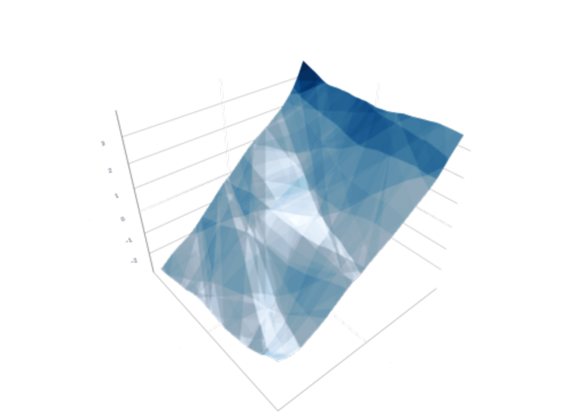
(b) $\lambda=10$

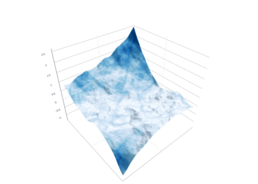
(c) $\lambda=100$

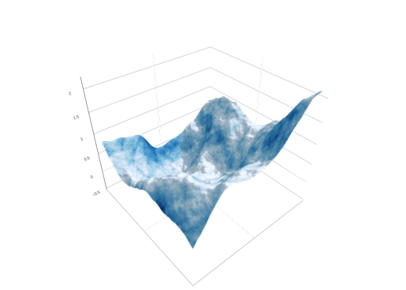
(d) $\lambda=1000$

Figure 3: $\mathbf{P}_{V}$ is Gaussian.

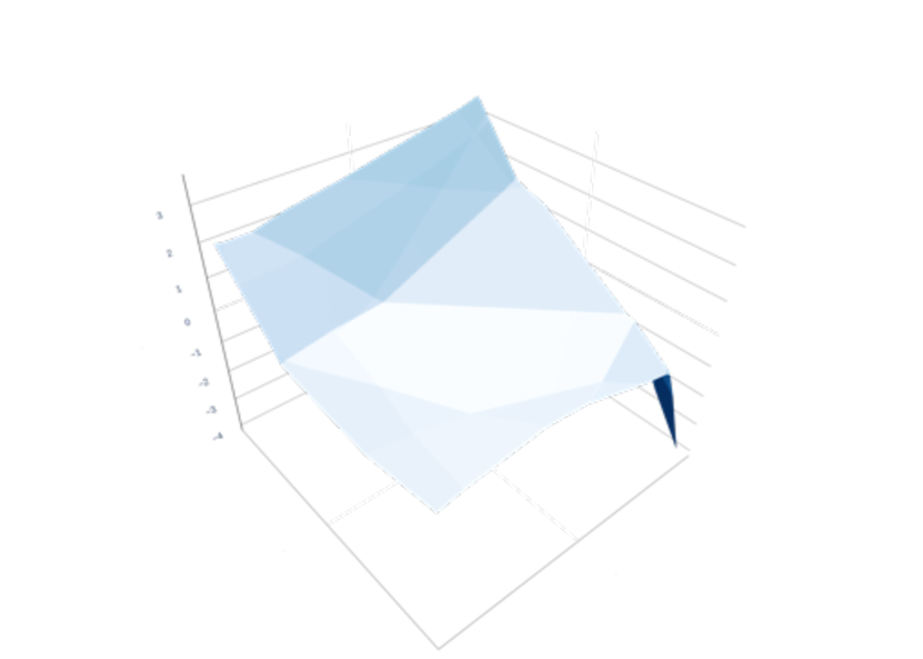
(a) $\lambda=1$

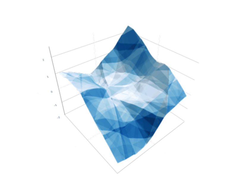
(b) $\lambda=10$

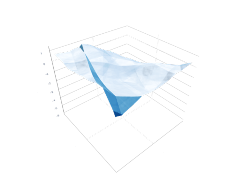
(c) $\lambda=100$

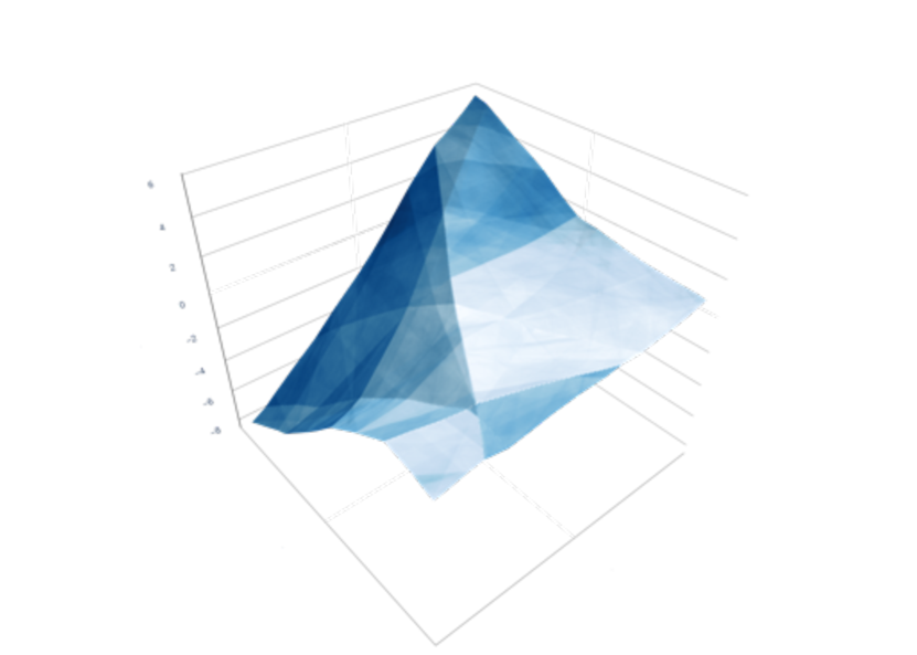
(d) $\lambda=1000$

Figure 4: $\mathbf{P}_{V}$ is symmetric ($\alpha=1.25$)-stable.

References

- Bartolucci et al. [2023] Francesca Bartolucci, Ernesto De Vito, Lorenzo Rosasco, and Stefano Vigogna. Understanding neural networks with reproducing kernel Banach spaces. Applied and Computational Harmonic Analysis, 62:194–236, 2023.
- Biermé et al. [2018] Hermine Biermé, Olivier Durieu, and Yizao Wang. Generalized random fields and Lévy’s continuity theorem on the space of tempered distributions. Communications on Stochastic Analysis, 12(4):4, 2018.
- Daley and Vere-Jones [2007] Daryl J. Daley and David Vere-Jones. An Introduction to the Theory of Point Processes: Volume II: General Theory and Structure. Probability and Its Applications. Springer New York, 2007.
- Duttweiler and Kailath [1973] Donald L. Duttweiler and Thomas Kailath. RKHS approach to detection and estimation problems–IV: Non-Gaussian detection. IEEE Transactions on Information Theory, 19(1):19–28, 1973.
- Dyer and Gur-Ari [2020] Ethan Dyer and Guy Gur-Ari. Asymptotics of wide networks from Feynman diagrams. In International Conference on Learning Representations, 2020.
- Fageot and Unser [2019] Julien Fageot and Michael Unser. Scaling limits of solutions of linear stochastic differential equations driven by Lévy white noises. Journal of Theoretical Probability, 32(3):1166–1189, 2019.
- Fageot et al. [2014] Julien Fageot, Arash Amini, and Michael Unser. On the continuity of characteristic functionals and sparse stochastic modeling. Journal of Fourier Analysis and Applications, 20:1179–1211, 2014.
- Fageot et al. [2020] Julien Fageot, Virginie Uhlmann, and Michael Unser. Gaussian and sparse processes are limits of generalized Poisson processes. Applied and Computational Harmonic Analysis, 48(3):1045–1065, 2020.
- Fernique [1967] Xavier Fernique. Processus linéaires, processus généralisés. Annales de l’institut Fourier, 17(1):1–92, 1967.
- Garriga-Alonso et al. [2019] Adrià Garriga-Alonso, Carl Edward Rasmussen, and Laurence Aitchison. Deep convolutional networks as shallow Gaussian processes. In International Conference on Learning Representations, 2019.
- Gelfand [1955] Izrail M. Gelfand. Generalized random processes. Dokl. Akad. Nauk SSSR (N.S.), 100:853–856, 1955.
- Gelfand and Shilov [1964] Izrail M. Gelfand and Georgiy E. Shilov. Generalized functions. Vol. I: Properties and operations. Academic Press, 1964.
- Gelfand and Vilenkin [1964] Izrail M. Gelfand and Naum Ya. Vilenkin. Generalized functions, Vol. 4: Applications of harmonic analysis. Academic Press, 1964.
- Gelfand et al. [1966] Izrail M. Gelfand, Mark I. Graev, and Naum Ya. Vilenkin. Generalized functions. Vol. 5: Integral geometry and representation theory. Academic Press, 1966.
- Hanin [2023] Boris Hanin. Random neural networks in the infinite width limit as Gaussian processes. The Annals of Applied Probability, 33(6A):4798–4819, 2023.
- Helgason [2011] Sigurdur Helgason. Integral Geometry and Radon Transforms. Springer New York, 2011.
- Hida and Ikeda [1967] Takeyuki Hida and Nobuyuki Ikeda. Analysis on Hilbert space with reproducing kernel arising from multiple Wiener integral. In Proc. Fifth Berkeley Sympos. Math. Statist. and Probability, pages 117–143. Univ. California Press, Berkeley, CA, 1967.
- Itô [1954] Kiyosi Itô. Stationary random distributions. Memoirs of the College of Science. University of Kyoto. Series A. Mathematics, 28:209–223, 1954.
- Itô [1984] Kiyosi Itô. Foundations of stochastic differential equations in infinite dimensional spaces, volume 47. SIAM, 1984.
- Jacob and Schilling [2001] Niels Jacob and René L. Schilling. Lévy-Type Processes and Pseudodifferential Operators, pages 139–168. Birkhäuser Boston, Boston, MA, 2001. ISBN 978-1-4612-0197-7.
- Kolmogorov [1935] Andrei N. Kolmogorov. La transformation de Laplace dans les espaces linéaires. CR Acad. Sci. Paris, 200:1717–1718, 1935.
- Lee et al. [2018] Jaehoon Lee, Yasaman Bahri, Roman Novak, Samuel S. Schoenholz, Jeffrey Pennington, and Jascha Sohl-Dickstein. Deep neural networks as Gaussian processes. In International Conference on Learning Representations, 2018.
- Ludwig [1966] Donald Ludwig. The Radon transform on Euclidean space. Communications on Pure and Applied Mathematics, 19:49–81, 1966.
- Mandelbrot and Van Ness [1968] Benoit B. Mandelbrot and John W. Van Ness. Fractional Brownian motions, fractional noises and applications. SIAM Review, 10(4):422–437, 1968.
- Matthews et al. [2018] Alexander G. de G. Matthews, Jiri Hron, Mark Rowland, Richard E. Turner, and Zoubin Ghahramani. Gaussian process behaviour in wide deep neural networks. In International Conference on Learning Representations, 2018.
- Minlos [1959] Robert A. Minlos. Generalized random processes and their extension in measure. Trudy Moskovskogo Matematicheskogo Obshchestva, 8:497–518, 1959.
- Neal [1996] Radford M. Neal. Bayesian Learning for Neural Networks. Lecture Notes in Statistics. Springer New York, 1996.
- Novak et al. [2019] Roman Novak, Lechao Xiao, Yasaman Bahri, Jaehoon Lee, Greg Yang, Daniel A. Abolafia, Jeffrey Pennington, and Jascha Sohl-Dickstein. Bayesian deep convolutional networks with many channels are Gaussian processes. In International Conference on Learning Representations, 2019.
- Ongie et al. [2020] Greg Ongie, Rebecca Willett, Daniel Soudry, and Nathan Srebro. A function space view of bounded norm infinite width ReLU nets: The multivariate case. In International Conference on Learning Representations, 2020.
- Parhi and Nowak [2021] Rahul Parhi and Robert D. Nowak. Banach space representer theorems for neural networks and ridge splines. Journal of Machine Learning Research, 22(43):1–40, 2021.
- Parhi and Nowak [2022] Rahul Parhi and Robert D. Nowak. What kinds of functions do deep neural networks learn? Insights from variational spline theory. SIAM Journal on Mathematics of Data Science, 4(2):464–489, 2022.
- Parhi and Nowak [2023a] Rahul Parhi and Robert D. Nowak. Near-minimax optimal estimation with shallow ReLU neural networks. IEEE Transactions on Information Theory, 69(2):1125–1140, 2023a.
- Parhi and Nowak [2023b] Rahul Parhi and Robert D. Nowak. Deep learning meets sparse regularization: A signal processing perspective. IEEE Signal Processing Magazine, 40(6):63–74, 2023b.
- Ramm and Katsevich [1996] Alexander G. Ramm and Alexander I. Katsevich. The Radon transform and local tomography. CRC Press, Boca Raton, FL, 1996.
- Rudin [1991] Walter Rudin. Functional analysis. International Series in Pure and Applied Mathematics. McGraw-Hill, Inc., New York, second edition, 1991.
- Sato [1999] Ken-Iti Sato. Lévy Processes and Infinitely Divisible Distributions. Cambridge Studies in Advanced Mathematics. Cambridge University Press, 1999.
- Unser [2023] Michael Unser. Ridges, neural networks, and the Radon transform. Journal of Machine Learning Research, 24(37):1–33, 2023.
- Unser et al. [2014] Michael Unser, Pouya D. Tafti, and Qiyu Sun. A unified formulation of Gaussian versus sparse stochastic processes—Part I: Continuous-domain theory. IEEE Transactions on Information Theory, 60(3):1945–1962, 2014.
- Williams [1996] Christopher Williams. Computing with infinite networks. Advances in Neural Information Processing Systems, 9, 1996.
- Yaida [2020] Sho Yaida. Non-Gaussian processes and neural networks at finite widths. In Mathematical and Scientific Machine Learning, pages 165–192. PMLR, 2020.
- Yang [2019] Greg Yang. Tensor programs I: Wide feedforward or recurrent neural networks of any architecture are Gaussian processes. Advances in Neural Information Processing Systems, 32, 2019.