Interplay between Domain Walls in Type-II Superconductors
and Gradients of Temperature/Spin Density

Abstract

We theoretically investigate the motion of a domain wall in type-II superconductors driven by inhomogeneities of temperature or spin density. The model consists of the time-dependent Ginzburg-Landau equation and the thermal/spin diffusion equation whose transport coefficients (the thermal/spin conductivity and the spin relaxation time) depend on the order parameter, interpolating the values for the superconducting and the normal states. Both numerical and analytical calculations suggest that the domain wall moves toward the higher temperature/spin-density region where the order parameter is suppressed. Both motions can be understood as dynamical processes minimizing the loss of the condensation energy. We also clearly define the forces on the domain wall according to their origins.

I Introduction

Among the vast field of research on superconductivity, studies involving quantum vortices, in particular, have been a central interest for many researchers. Vortices can be regarded as singularities in the phase of the order parameter and stably behave as topologically defected particle-like objects under magnetic fields. They are not only prominent in understanding transport properties such as electric resistance of the superconducting systems, but also play a vital role in the Berezinskii-Kosterlitz-Thouless (BKT) transition [1, 2, 3], known as the mechanism of the superfluid transition in two-dimensional systems. In addition, there are many condensed matter systems in which the motion of topological defects becomes important, such as superfluid helium and skyrmions in chiral magnets to which some theoretical applications can be expected [4]. Therefore, enhancing the possibilities of controlling vortex motion in superconductors is the greatest advantage from both an academic interest and an application perspective, and it is potentially available to all those engaged in these fields.

The most common way to drive vortices in type-II superconductors, which has long been studied [5, 6, 7, 8, 9, 10, 11, 12, 13, 14, 15, 16, 17], is to apply the transport electric currents $\bm{J}_{\textrm{tr}}$. We thus begin by reviewing currently established understanding of the driving force acting on an isolated quantum vortex by the transport current. It has been assumed that the driving force per unit length along the magnetic field is given by the following equation in the SI units:

$$\bm{F}_{\textrm{drv}}=\bm{J}_{\textrm{tr}}\times\bm{\phi}_{0},$$ (1)

where $\bm{\phi}_{0}$ is a vector along the vortex axis whose amplitude is $h/(2\lvert e\rvert)$. $h$ and $\lvert e\rvert$ denote the Planck constant and the the charge unit respectively. This force is often conventionally referred to as the ‘Lorentz force’. However, the question of whether its physical origin is the same as the ‘Lorentz force’ that drives charges with finite velocity under a magnetic field has caused long-standing controversy; Some studies have argued that there must be some contribution from a hydrodynamic force: the ‘Magnus force’, which acts on a rotating object in a flow [18, 19, 20, 21].

In the framework of the time-dependent Ginzburg-Landau (TDGL) equation [9, 22], we have recently presented a clear description to this question [16, 17]. In this work, the forces on an isolated vortex are defined as the net momentum per unit time flowing into the region surrounding the vortex. The magnetic force and the hydrodynamic force are respectively expressed as the surface integral of the Maxwell stress tensor and the momentum flux tensor derived from the TDGL equation and the Ampère’s law. Each contribution depends on the integral region and thus cannot be regarded as a force, as itself, on the vortex core. However, the sum of these two forces becomes independent of the integral region and can be defined as a driving force on the vortex. Therefore, the answer to the previous question is that only the sum of the magnetic and hydrodynamic forces is a physically meaningful force on a vortex. The conclusions presented here were soon extended in [17]. By solving the same equations numerically under the finite GL parameters, it was found that the value of the driving force that was previously known had to be corrected by multiplying it by a numerical factor.

Hence, the method based on the TDGL equation and the momentum balance relation derived from it to define the forces on the isolated vortex was a significant achievement in settling the long controversy. We focused on the possibilities of this scheme to examine alternative transport methods, such as heat flows induced by temperature gradients and spin currents induced by spin accumulation gradients. Brief overviews of the current understanding of the motion of vortices under each current is given in the following two paragraphs.

heat flow

The history of research on the motion of vortices under temperature gradients can be traced back in the 1960s [23, 24, 25, 26, 27, 28, 29, 30, 31, 32, 33]. The pioneering theoretical work was done by Stephen [24], in which an expression for the effective thermal force on a vortex line was derived based on thermodynamic considerations. This expression is given by

$$\bm{F}_{\textrm{th}}=-\frac{\phi_{0}S}{B}\nabla T,$$ (2)

where $S$ is the entropy, and $B$ is the magnetic induction. This expression shows that the thermal force is oriented opposite to the temperature gradient. Therefore, he stated that the vortex is driven from the hotter to the colder region. An equation similar to Eq. (2) was written by Yntema in [28]. In Stephen’s paper, the coefficient $-\frac{\phi_{0}S}{B}$ which appears in Eq. (2) is simply explained as “the entropy of unit length of a vortex line”. However, it is not immediately evident how this can be related to what is currently known as “the transport entropy”, as pointed out in [29].

At the same time, the thermoelectric effects (the Nernst and Ettingshausen effects) in vortex systems were experimentally investigated [25, 29, 26, 30]. It was consistently assumed that vortices under a temperature gradient would move toward the lower temperature region.

Studies on similar systems have been continued to the present day. However, in recent years, there have been reports from several viewpoints including theoretical [34], experimental [35], and numerical studies [36, 37], suggesting that the vortices would move to or located on the higher temperature region.

In 2010, Sergeev et al. derived the effective thermal force [34]. They highlighted the significance of the magnetization current induced by the temperature gradient, a factor that the authors in [34] claimed to be. The ‘Lorentz force’ , which arises from this current, was identified to be directed from the colder to the hotter region.

Following the study, Veshchunov et al. carried out experiments aimed at thermally controlling quantum vortices [35]. This experiment revealed that the local temperature gradient generated by the laser drives the vortices and attracts them in the direction of the laser spot (i.e., the local high temperature region), allowing them to be easily positioned. This implies that driving vortices driven by temperature gradients have the potential to be carried out with high speed and precision [35].

Duarte et al. [36] and de Toledoet al. [37] numerically solved the TDGL equation under a uniform temperature gradient, and reported that the vortices begin to form in the hotter region when the magnetic field is sufficiently weak.

Taking into account these situations, we currently have two crucial issues which still remain unresolved.

1. There is a lack of consensus among previous studies regarding the direction of motion of superconducting vortices under a temperature gradient.

2. The origin of the thermal force is to be clarified. In particular, it is necessary to establish the precise and quantitative definition of the thermal force based on the law of momentum conservation.

spin current

Another possible way to drive vortices is the use of spin currents. In recent years spintronics in superconductors has attracted many researchers’ attention [38, 39, 40, 41, 42, 43, 44, 45]. However, understanding of the driving force on a vortex due to the spin currents is not well established and thus further research is desirable.

In order to address these issues, we start with a more tractable target. In this paper, we investigate one-dimensional systems where a domain wall, rather than a vortex, flows under different currents: heat flow and spin current. The goal of this paper is to describe the motion of the domain wall and propose more preferable definitions of the forces on it than that currently in use. We utilize the TDGL equation, which has successfully described the properties of vortices in the flux flow state as mentioned above, and diffusion equations for the temperature or spin accumulation.

In Sec. II, we introduce the model for the case with a temperature gradient, and both numerical and analytical calculations perform. The results of these calculations show a good agreement with each other. In Sec. III, we address the system with spin accumulation gradient, and the discussion proceeds in a similar manner. In Sec. IV, we discuss some possible applications of our analyses. Sec. V presents a summary of the main results and their interpretation.

II motion of domain wall under temperature gradient

In this section, we discuss the motion of a domain wall in a one-dimentinal superconductor system with a finite length under a temperature gradient, using the TDGL equation. The equation of motion for the temperature is the standard thermal diffusion equation, which forms a boundary value problem of simultaneous differential equations together with the TDGL equation. We investigate the model both numerically and analytically.

II.1 Model

We consider a superconductor under a temperature gradient in the framework of the Ginzburg-Landau theory. All physical quantities depend only on the $x$-coordinate and are isotropic in the $y,z$-axis directions. Hence, the problem becomes a one-dimensional boundary value problem defined in the region $x_{\textrm{L}}\leq x\leq x_{\textrm{R}}$. For the sake of simplicity, in this paper, our discussion is limited to the case of $x_{\textrm{L}}=-x_{\textrm{R}}$.

II.1.1 TDGL. equation

In the ordinary Ginzburg-Landau theory, the free energy $F$ per unit area on the $yz$-plane of the system can be written as follows:

$$F =\int_{x_{\textrm{L}}}^{x_{\textrm{R}}}\text{d}x\;\left[\frac{\hbar^{2}}{2m}\left(\frac{\text{d}\Psi(x)}{\text{d}x}\right)^{2}\right.$$

$$\left.\hskip 8.5359pt+\alpha_{0}\frac{T(x)-T_{\textrm{c}}}{T_{\textrm{c}}}\Psi^{2}(x)+\frac{\beta}{2}\Psi^{4}(x)\right].$$ (3)

Here, $\Psi(x)$ denotes the condensate wavefunction, whose dimension is $(\textrm{volume})^{-1/2}$. We can take $\Psi(x)$ as real, due to the absence of the magnetic field. $m,\hbar$ is the mass of a Cooper pair, Planck constant devided by 2$\pi$, respectively. $\alpha_{0},\beta$ are positive constants independent of the temperature and the position. $T_{\textrm{c}}$ is the critical temperature. Taking the variational of the free energy gives the Ginzburg-Landau equation,

$$-\frac{\hbar^{2}}{2m}\frac{\text{d}^{2}\Psi(x)}{\text{d}x^{2}}+\alpha_{0}\frac{T(x)-T_{\textrm{c}}}{T_{\textrm{c}}}\Psi(x)+\beta\Psi^{3}(x)=0.$$ (4)

To discuss the dynamics of the domain wall, we introduce the time dependency of the order parameter $\Psi(x,t)$ and temperature $T(x,t)$. Then we assume that the time development is governed by the following TDGL equation:

$${-\frac{\hbar^{2}}{2m}\frac{\partial^{2}\Psi(x,t)}{\partial x^{2}}+\alpha_{0}\frac{T(x,t)-T_{\textrm{c}}}{T_{\textrm{c}}}\Psi(x,t)+\beta\Psi^{3}(x,t)}$$

$$=-\gamma\frac{\partial\Psi(x,t)}{\partial t},$$ (5)

where $\gamma(>0)$ in the RHS is a relaxation coefficient. The boundary conditions are imposed in the form of

$$\displaystyle T\left(x_{\textrm{L}},t\right) =T_{\textrm{L}}$$ (6a)

$$\displaystyle T\left(x_{\textrm{R}},t\right) =T_{\textrm{R}}$$ (6b)

for the temperature with $T_{\textrm{L}},\ T_{\textrm{R}}<T_{\textrm{c}}$, and

$$\displaystyle\Psi\left(x_{\textrm{L}},t\right) =-\sqrt{\frac{\alpha_{0}}{\beta}\frac{T_{\textrm{L}}-T_{\textrm{c}}}{T_{c}}}$$ (7a)

$$\displaystyle\Psi\left(x_{\textrm{R}},t\right) =+\sqrt{\frac{\alpha_{0}}{\beta}\frac{T_{\textrm{R}}-T_{\textrm{c}}}{T_{\textrm{c}}}}$$ (7b)

for the order parameter. The RHSs of Eqs. (7a) and (7b) are set to the values that the order parameter takes in the bulk in thermal equilibrium under the local temperature. The different signs guarantee that a domain wall exists somewhere between Eqs. (7a) and (7b) in the region.

For later convenience, we rewrite the TDGL equation into the dimensionless form as

$${-\xi^{2}\frac{\partial^{2}\psi(x,t)}{\partial x^{2}}+\frac{\tau(x,t)-1}{1-\tau_{\textrm{L}}}\psi(x,t)+\psi^{3}(x,t)}$$

$$=-\tilde{\gamma}\frac{\partial\psi(x,t)}{\partial t}.$$ (8)

Here,

$$\psi(x,t)\equiv\displaystyle\frac{\Psi(x,t)}{\sqrt{\displaystyle\frac{\alpha_{0}}{\beta}\frac{T_{\textrm{L}}-T_{\textrm{c}}}{T_{c}}}}$$ (9)

and

$$\tau(x,t)\equiv\displaystyle\frac{T(x,t)}{T_{\textrm{c}}}$$ (10)

are the dimensionless order parameter and temperature, respectively. The symbol $\xi\equiv\sqrt{\hbar^{2}T_{\textrm{c}}/2m\alpha_{0}(T_{\textrm{c}}-T_{\textrm{L}})}$ denotes the coherence length and $\tilde{\gamma}\equiv\gamma T_{\textrm{c}}/\alpha_{0}(T_{\textrm{c}}-T_{\textrm{L}})$ denotes the relaxation coefficient in the dimensionless TDGL Eq. (II.1.1). We assume $\xi\ll x_{\textrm{R}}$.

The boundary conditions Eqs. (6) and (7) also are rewritten in the dimensionless expressions as

$$\tau(x_{\textrm{L}},t) =\tau_{\textrm{L}}$$ (11a)

$$\tau(x_{\textrm{R}},t) =\tau_{\textrm{R}}$$ (11b)

$$\psi(x_{\textrm{L}},t) =-1$$ (11c)

$$\psi(x_{\textrm{R}},t) =\displaystyle+\sqrt{\frac{1-\tau_{\textrm{R}}}{1-\tau_{\textrm{L}}}}.$$ (11d)

II.1.2 Thermal diffusion equation

Another equation of motion is the one-dimensional thermal diffusion equation:

$$-\frac{\partial}{\partial x}\left[-\kappa(x,t)\frac{\partial T(x,t)}{\partial x}\right]=C\frac{\partial T(x,t)}{\partial t},$$ (12)

where $C$ is the specific heat. The symbol $\kappa(x,t)$ denotes the thermal conductivity which spatially and temporally varies. We assume that the thermal conductivity $\kappa(x,t)$ depends on the order parameter to reflect the fact that the value for the superconducting state $\kappa_{\textrm{s}}$ is lower than that for the normal state $\kappa_{\textrm{n}}$. Therefore, we assume the phenomenological expression for the thermal conductivity:

$$\kappa(x,t)=\kappa_{\textrm{n}}+\left(\kappa_{\textrm{s}}-\kappa_{\textrm{n}}\right)\psi^{2}(x,t).$$ (13)

According to this formula, $\kappa=\kappa_{\textrm{n}}$ when $\psi=0$ and $\kappa=\kappa_{\textrm{s}}$ when $\psi=1$ respectively, interpolating the two values.

The dimensionless expression for Eq. (12) is given as

$${\frac{\partial}{\partial x}\left[\left\{1+(k-1)\psi^{2}(x,t)\right\}\frac{\partial\tau(x,t)}{\partial x}\right]}$$

$$=\frac{C}{\kappa_{\textrm{n}}}\frac{\partial\tau(x,t)}{\partial t},$$ (14)

where $k\equiv\kappa_{\textrm{s}}/\kappa_{\textrm{n}}$ is the ratio of the thermal conductivity for the superconducting and normal state.

II.1.3 summary of the problem

We solve the TDGL Eq. (II.1.1) and the thermal diffusion Eq. (II.1.2) with the boundary conditions Eqs. from (11a) to (11d).

II.2 Numerical simulation

Let us begin by solving the equations numerically. The explicit Euler method is employed as a numerical method, whereby the solution is updated from the initial state which satisfies the boundary conditions. The results of a series of the simulations are shown in FIG. 1 for the parameters $k=0.5$, $\tilde{\gamma}\kappa_{\textrm{n}}/(C\xi^{2})=1$, $\tau_{\textrm{L}}=0.990$, and $\tau_{\textrm{R}}=0.995$. The snapshots (a) to (d) are arranged in order of time evolution. The horizontal axis represents the length measured in units of the coherence length, and the size of the system is set to 50 times the coherence length (i.e., $x_{\textrm{R}}=25$). The value of the order parameter is represented on the vertical axis, with the blue line indicating the solution, and the red dashed line indicating where the order parameter vanishes. The defect is located at the crossing point of the red dashed line and the blue line. The domain wall is formed where the order parameter varies drastically within a region of the order of the coherence length. The domain wall, from a given initial state, with a characteristic shape immediately forms and moves up against the heat flow toward the hotter region. During the motion, the domain wall keeps moving straight toward the higher temperature boundary, and no oscillating behaviour is observed.

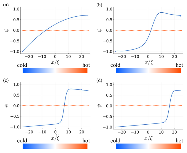
Figure 1: Numerical solutions of the TDGL Eq. (II.1.1) coupled with the thermal diffusion Eq. (II.1.2). (a) The given initial state satisfying the boundary conditions Eqs. (11c) and (11d). (b) The initial state immediately is re-formed and the domain wall-like structure is found. (c), (d) The domain wall keeps on flowing against the heat flow. Note that the coloured bands under the horizontal axes symbolically indicate the presence of a temperature gradient, but are not exact reflections of the solution.

II.3 Analytical calculation

The numerical results indicate that, within our model, the domain wall moves toward the region with the higher temperature. The reason for this will now be demonstrated analytically. In the following section, we consider a flow state in which the domain wall far from the boundaries of the system moves slowly with a constant velocity $v$. The goals of this section are followings. (1) To provide explicit definitions of forces on the domain wall. (2) To derive the relation that links the velocity $v$ and the heat flow $q=-\kappa\partial\tau/\partial x$ to explain the direction of motion which the numerical simulation shows.

II.3.1 method

The strategy is the linearization of the variables with respect to $v$ [9, 11, 12]. The order parameter $\psi(x,t)$ and the temperature $\tau(x,t)$ are expanded as follows with respect to $v$:

$$\begin{split}\psi(x,t)&=\psi_{0}(x-vt)+\psi_{1}(x)+\mathcal{O}(v^{2})\\ &=\psi_{0}(x)+\left(-vt\frac{\text{d}\psi_{0}(x)}{\text{d}x}+\psi_{1}(x)\right)+\mathcal{O}(v^{2})\end{split}$$

$$=\psi_{0}(x)+\phi_{1}(x,t)+\mathcal{O}(v^{2})$$ (15)

and

$$\begin{split}\tau(x,t)&=\tau_{0}(x-vt)+\tau_{1}(x)+\mathcal{O}(v^{2})\end{split}$$

$$=\tau_{\textrm{L}}+\tau_{1}(x)+\mathcal{O}(v^{2}).$$ (16)

The subscripts 0 or 1 denote the order of the velocity $v$. Therefore, $\psi_{0}$ and $\tau_{0}$ are the equilibrium solutions when we set $\tau_{0}(x,t)=\tau_{\textrm{L}}$. The explicit expression for $\psi_{0}(x)$ is given in Appendix A. The solutions to our equations are expressed as the sum of the translation of the solutions in equilibrium: ($\psi_{0}$, $\tau_{0}$) and the modulation components: ($\psi_{1}$, $\tau_{1}$). The function $\phi_{1}(x,t)\equiv-vt\frac{\text{d}\psi_{0}(x)}{\text{d}x}+\psi_{1}(x)$ includes all the first order contributions with respect to $v$ in $\psi(x,t)$. In discussion below, the terms in $\mathcal{O}(v^{2})$ are neglected.

By substituting these expansions Eqs. (II.3.1) and  (II.3.1) into Eqs. (II.1.1) and (II.1.2), the relations for each order of the velocity $v$ can be obtained. However, the relations for the 0th order are trivial because the results are the Ginzburg-Landau equation in equilibrium from Eq. (II.1.1) and an identity from Eq. (II.1.2). The following subsections discuss the first-order relations for $v$.

II.3.2 linearization of the TDGL equation

The linearization of the TDGL equation (II.1.1) yields

$$\hat{L}\phi_{1}(x,t)+\frac{\psi_{0}(x)\tau_{1}(x)}{1-\tau_{\textrm{L}}}=\tilde{\gamma}v\frac{\text{d}\psi_{0}(x)}{\text{d}x},$$ (17)

where the linear operator $\hat{L}\equiv-\xi^{2}\frac{\partial^{2}}{\partial x^{2}}-1+3\psi_{0}^{2}(x)$ is introduced. By multiplying Eq. (17) by $\frac{\text{d}\psi_{0}(x)}{\text{d}x}$, we obtain

$${-\xi^{2}\frac{\partial}{\partial x}\left[\frac{\text{d}\psi_{0}(x)}{\text{d}x}\frac{\partial\phi_{1}(x,t)}{\partial x}-\frac{\text{d}^{2}\psi_{0}(x)}{\text{d}x^{2}}\phi_{1}(x,t)\right]}$$

$$-\tilde{\gamma}v\left(\frac{\text{d}\psi_{0}(x)}{\text{d}x}\right)^{2}+\frac{\tau_{1}(x)}{2(1-\tau_{\textrm{L}})}\frac{\text{d}}{\text{d}x}\psi_{0}^{2}(x)=0.$$ (18)

This equation corresponds to the equation called “the local momentum balance relation” derived in [16]. The detailed derivation of Eq. (II.3.2) and its physical meaning as the local momentum balance relation, as the previous study [16, 17] showed, are given in Appendix B.

II.3.3 linearization of the thermal diffusion equation

The first-order relation, obtained from the thermal diffusion equation, is as follows:

$$\frac{\text{d}}{\text{d}x}\left[\left\{1+(k-1)\psi_{0}^{2}(x)\right\}\frac{\text{d}\tau_{1}(x)}{\text{d}x}\right]=0.$$ (19)

It is more convenient to use the notation of the one-dimensional heat flow $q(x,t)$ defined as

$$q(x,t)\equiv-\kappa(x,t)\frac{\partial T(x,t)}{\partial x},$$ (20)

and by expanding $q(x,t)$ with respect to $v$ in the same way as the case for Eq. (II.1.1) and Eq. (II.1.2), we easily obtain

$${q(x,t)=-\kappa_{n}T_{\textrm{c}}\left\{1+(k-1)\psi_{0}^{2}(x)\right\}\frac{\text{d}\tau_{1}(x)}{\text{d}x}}$$

$$+\mathcal{O}(v^{2}),$$ (21)

which is obviously related to Eq. (19). This expression shows that the heat flow is temporally uniform up to the first order of $v$. Discarding the term in $\mathcal{O}(v^{2})$ and combining Eq. (II.3.3) with Eq. (19), the relation is simplified as

$$\frac{\partial q(x,t)}{\partial x}=0,$$ (22)

which implies that the heat flow is not only temporally but also spatially uniform. Hence, we can introduce a constant $q$ satisfying

$$\tau_{1}(x)=\frac{-q}{\kappa_{\textrm{n}}T_{\textrm{c}}}\int_{x_{\textrm{L}}}^{x}\frac{\text{d}x^{\prime}}{1+(k-1)\psi_{0}^{2}(x^{\prime})}.$$ (23)

The spatial distribution of temperature is determined by this integral equation Eq. (23).

II.3.4 forces on domain wall

Each term on the LHS of the local momentum balance relation Eq. (II.3.2) in our model represents force densities which are localized at the region near the domain wall because both of the second and the third terms include the spatial derivatives of the order parameter in equilibrium, and thus also the first term is localized at the region near the domain wall. This fact guarantees that the integrals of these terms over the whole system give the forces on the domain wall because the integrands become independent of the size of the system if it is enough larger than $\xi$. Then the forces on the domain wall are well-defined in a physically meaningful manner and classified into three types according to their origins.

driving force

The first term on the LHS of Eq. (II.3.2) has a spatial derivative over the entire term, and its integral defines the net momentum that enters and exits through the boundaries, namely the driving force. The integral of the term that includes $\frac{\text{d}\psi_{0}(x)}{\text{d}x}$ does not contribute to the surface term because of the boundary conditions Eqs. (56). Therefore, we can define and evaluate the driving force as

$$\begin{split}F_{\textrm{drv}}&\equiv-\xi^{2}\int_{x_{\textrm{L}}}^{x_{\textrm{R}}}d\text{d}x \;\frac{\partial}{\partial x}\left[\frac{\text{d}\psi_{0}(x)}{\text{d}x}\frac{\partial\phi_{1}(x,t)}{\partial x}\right.\\ &\left.\hskip 54.06006pt-\frac{\text{d}^{2}\psi_{0}(x)}{\text{d}x^{2}}\phi_{1}(x,t)\right]\end{split}$$

$$=-\xi^{2}\left.\frac{\text{d}^{2}\psi_{0}(x)}{\text{d}x^{2}}\right|_{x=x_{\textrm{R}}}\left(1-\sqrt{\frac{1-\tau_{\textrm{R}}}{1-\tau_{\textrm{L}}}}\right).$$ (24)

viscous force

The second term on the LHS of Eq. (II.3.2) has a negative sign and $v$, so the integral can be considered as a viscous force on the domain wall

$$F_{\textrm{vis}}\equiv-\tilde{\gamma}v\int_{x_{\textrm{L}}}^{x_{\textrm{R}}}\text{d}x\;\left(\frac{\text{d}\psi_{0}(x)}{\text{d}x}\right)^{2}.$$ (25)

thermal force

The thermal force is defined as the integral of the third term on the LHS of Eq. (II.3.2) as

$$F_{\textrm{th}}\equiv\frac{1}{2(1-\tau_{\textrm{L}})}\int_{x_{\textrm{L}}}^{x_{\textrm{R}}}\text{d}x\;\tau_{1}(x)\frac{\text{d}}{\text{d}x}\psi_{0}^{2}(x).$$ (26)

II.3.5 force-balance

The sum of these forces is equal to 0. Using the notations defined above, the force-balance relation can be written as

$$F_{\textrm{drv}}+F_{\textrm{vis}}+F_{\textrm{th}}=0.$$ (27)

II.3.6 linear relation between $v$ and $q$

$F_{\textrm{drv}}$ and $F_{\textrm{th}}$ can be expressed in terms of the heat flow. First, when we let $x=x_{\textrm{R}}$ in Eq. (23), the temperature difference between boundaries is given by

$$\tau_{\textrm{R}}-\tau_{\textrm{L}}=\frac{-q}{\kappa_{\textrm{n}}T_{\textrm{c}}}\int_{x_{\textrm{L}}}^{x_{\textrm{R}}}\frac{\text{d}x}{1+(k-1)\psi_{0}^{2}(x)}.$$ (28)

Substituting this into the definition of $F_{\textrm{drv}}$ Eq. (II.3.4), we obtain

$${-\xi^{2}\left.\frac{\text{d}^{2}\psi_{0}(x)}{\text{d}x^{2}}\right|_{x=x_{\textrm{R}}}\left(1-\sqrt{\frac{1-\tau_{\textrm{R}}}{1-\tau_{\textrm{L}}}}\right)}$$

$$=\frac{-\xi^{2}\left(\tau_{\textrm{R}}-\tau_{\textrm{L}}\right)}{\sqrt{1-\tau_{\textrm{L}}}\left(\sqrt{1-\tau_{\textrm{R}}}+\sqrt{1-\tau_{\textrm{L}}}\right)}\left.\frac{\text{d}^{2}\psi_{0}(x)}{\text{d}x^{2}}\right|_{x=x_{\textrm{R}}}$$

$$=\frac{q\eta}{2\left(1-\tau_{\textrm{L}}\right)\kappa_{\textrm{n}}T_{\textrm{c}}}\int_{x_{\textrm{L}}}^{x_{\textrm{R}}}\frac{\text{d}x}{1+(k-1)\psi_{0}^{2}\left(x\right)},$$ (29)

where

$$\eta\equiv 2\xi^{2}\frac{\sqrt{1-\tau_{\textrm{L}}}}{\left(\sqrt{1-\tau_{\textrm{R}}}+\sqrt{1-\tau_{\textrm{L}}}\right)}\left.\frac{\text{d}^{2}\psi_{0}(x)}{\text{d}x^{2}}\right|_{x=x_{\textrm{R}}}$$ (30)

is a negative constant. Next, the thermal force is evaluated. By performing the integral by parts in the definition of $F_{\textrm{th}}$ Eq. (26) and using Eq. (28) and Eq. (59), we have

$$F_{\textrm{th}} =\frac{-q}{2\left(1-\tau_{\textrm{L}}\right)\kappa_{\textrm{n}}T_{\textrm{c}}}\int_{x_{\textrm{L}}}^{x_{\textrm{R}}}\text{d}x\;\frac{\psi_{0}^{2}\left(x_{\textrm{R}}\right)-\psi_{0}^{2}\left(x\right)}{1+(k-1)\psi_{0}^{2}\left(x\right)}.$$ (31)

Finally, the force-balance relation Eq. (27), Eqs. (II.3.6) and (31) yield the linear relation between $v$ and $q$ as

$$v=\frac{-q}{2(1-\tau_{\textrm{L}})\tilde{\gamma}\kappa_{\textrm{n}}T_{\textrm{c}}}G[\psi_{0}(x)],$$ (32)

where

$$G[\psi_{0}(x)]\equiv\frac{\displaystyle\int_{x_{\textrm{L}}}^{x_{\textrm{R}}}\text{d}x\; \frac{\psi_{0}^{2}\left(x_{\textrm{R}}\right)-\psi_{0}^{2}\left(x\right)-\eta}{1+(k-1)\psi_{0}^{2}(x)}}{\displaystyle\int_{x_{\textrm{L}}}^{x_{\textrm{R}}}\text{d}x\; \left(\frac{\text{d}\psi_{0}(x)}{\text{d}x}\right)^{2}}.$$ (33)

The functional $G$ is always positive only if $k$ is smaller than $1$ because $\psi_{0}^{2}(x)\leq\psi_{0}^{2}(x_{\textrm{R}})\leq 1$. Hence, Eq. (32) shows that $v$ and $q$ have the different sign. In conclusion, within our framework, the domain wall moves from the lower to higher temperature region, not along, but against the heat flow. This statement is consistent with the results obtained from the numerical simulation shown in Eq. (II.2). This is the reason why Eq. (32) is considered as the theoretical basis for this phenomenon under conditions where the temperature gradient or heat flow is sufficiently weak.

II.4 Remarks

The signs of the domain wall’s velocity $v$, the heat flow $q$ and forces $F_{\textrm{drv}}$, $F_{\textrm{vis}}$, $F_{\textrm{th}}$ are easily determined. Equation (28) tells us $q<0$, so $v>0$ since they have different signs. It is obvious that $F_{\textrm{vis}}<0$ as it is against $v$. Equations (II.3.6) and (31) show $F_{\textrm{drv}}$, $F_{\textrm{th}}>0$. These results are summarized in FIG. 2.

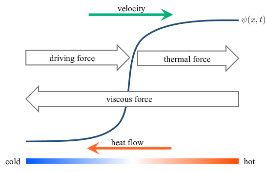
Figure 2: The illustration of the heat flow, velocity and three forces. According to Eq. (32), the domain wall’s velocity is directed to the hotter region since the heat flow is directed to the colder region. The viscous force is against the velocity, and the signs of the driving force and the thermal force can be determined by Eqs. (II.3.6) and (31) respectively.

The direction of the domain wall’s motion toward the higher temperature region can be understood in the same way as the pinning of vortices where defects or impurities locally reduce the order parameter of superconductivity and exert an attractive force on vortices. It is more energetically preferable when vortices are located at the center of pinning where superconductivity is broken. By analogy with this example of pinning, we can claim that the domain wall tends to move to the hotter region where the amplitude of the order parameter is likely to be smaller than that in the colder region to reduce the total energy, which makes it more stable (FIG. 3).

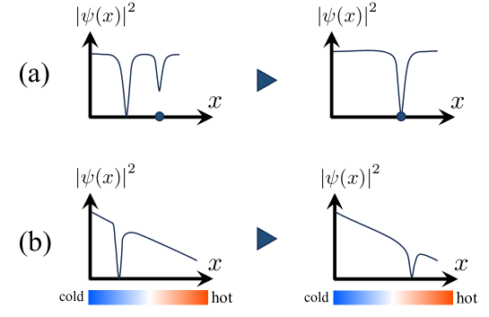
Figure 3: A comparison between the motion of the order parameters. (a) In the pinning effect, the defect tends to move to the pinning centers, such as impurities, represented by the dot on the horizontal axes. (b) The motion of the domain wall under a temperature gradient discussed so far. We find a similarity between the two cases as processes minimizing the loss of the condensation energy.

III motion of domain wall under spin-density gradient

In this section, we address the domain wall under the spin accumulation gradient. As in the previous section, we consider a one-dimensional superconductor in the finite region $x_{\textrm{L}}\leq x\leq x_{\textrm{R}}$. The model consists of the TDGL equation and the spin diffusion equation. The spatial variation of the spin accumulation affects the critical temperature [38, 43] in the TDGL equation. The microscopic derivation of the spin diffusion equation was presented in [40].

III.1 Model

We introduce the spin accumulation $\mu(x,t)$ and the spin accumulation-dependent critical temperature $T_{\textrm{c}}\left(\mu^{2}(x,t)\right)$. Here, it is assumed that the critical temperature is an even function of the spin accumulation because the spin $\uparrow$ and $\downarrow$ are equivalent in this model. The dimensionless TDGL equation is given by

$${-\xi^{2}\frac{\partial^{2}\psi(x,t)}{\partial x^{2}}+\frac{T-T_{\textrm{c}}\left(\mu^{2}(x,t)\right)}{T_{\textrm{c}}\left(\mu^{2}(x,t)\right)}\frac{T_{\textrm{c}}\left(0\right)}{T_{\textrm{c}}\left(0\right)-T}\psi(x,t)}$$

$$+\psi^{3}(x,t)=-\tilde{\gamma}\frac{\partial\psi(x,t)}{\partial t},$$ (34)

where the coherence length, the dimensionless order parameter and the relaxation coefficient are respectively defined as

$$\xi\equiv\sqrt{\frac{\hbar^{2}T_{\textrm{c}}\left(0\right)}{2m\alpha_{0}\left(T_{\textrm{c}}\left(0\right)-T\right)}}$$ (35)

$$\psi(x,t)\equiv\frac{\displaystyle\Psi(x,t)}{\sqrt{\frac{\displaystyle\alpha_{0}\left(T_{\textrm{c}}\left(0\right)-T\right)}{\displaystyle\beta T_{\textrm{c}}\left(0\right)}}}$$ (36)

$$\tilde{\gamma}\equiv\frac{\gamma}{\alpha_{0}}\frac{T_{\textrm{c}}\left(0\right)}{T_{\textrm{c}}\left(0\right)-T}.$$ (37)

Note that the temperature $T$ is a constant unlike the model discussed in the previous section.

In addition, we adopt the spin diffusion equation

$$\frac{\partial}{\partial x}\left[\sigma(x,t)\frac{\partial\mu(x,t)}{\partial x}\right]-\frac{\mu(x,t)}{\tau(x,t)}=\frac{\partial\mu(x,t)}{\partial t}.$$ (38)

Here, $\sigma(x,t)$ and $\tau(x,t)$ denote the spin conductivity and the spin relaxation time. Again, as we did before, we assume that these parameters spatially and temporally vary via the order parameter dependency given by

$$\sigma(x,t)=\sigma_{\textrm{n}}+\left(\sigma_{\textrm{s}}-\sigma_{\textrm{n}}\right)\psi^{2}(x,t)$$ (39)

$$\tau(x,t)=\tau_{\textrm{n}}+\left(\tau_{\textrm{s}}-\tau_{\textrm{n}}\right)\psi^{2}(x,t),$$ (40)

indicating that the values for the superconducting (with subscript s) and normal (with subscript n) states are interpolated.

Taking $\mu^{2}(x,t)$, instead of $\mu(x,t)$ itself, as a new variable, the spin diffusion equation Eq. (38) can be rewritten into the following form:

$${\frac{\partial}{\partial x}\left[\sigma(x,t)\frac{\partial\mu^{2}(x,t)}{\partial x}\right]-\frac{\sigma(x,t)}{2\mu^{2}(x,t)}\left(\frac{\partial\mu^{2}(x,t)}{\partial x}\right)^{2}}$$

$$-\frac{2\mu^{2}(x,t)}{\tau(x,t)}=\frac{\partial\mu^{2}(x,t)}{\partial t}.$$ (41)

We impose the boundary conditions for the spin accumulation as

$$\displaystyle\mu^{2}(x_{\textrm{L}},t) =0$$ (42a)

$$\displaystyle\mu^{2}(x_{\textrm{R}},t) =\mu^{2}_{\textrm{R}},$$ (42b)

and those for the dimensionless order parameter are given as

$$\displaystyle\psi(x_{\textrm{L}},t) =-1$$ (43a)

$$\displaystyle\psi(x_{\textrm{R}},t) =\displaystyle\sqrt{\frac{T_{\textrm{c}}\left(\mu^{2}_{\textrm{R}}\right)-T}{T_{\textrm{c}}\left(\mu^{2}_{\textrm{R}}\right)}\frac{T_{\textrm{c}}\left(0\right)}{T_{\textrm{c}}\left(0\right)-T}},$$ (43b)

which are the values for an equilibrium state in the bulk (See Eq. (7).) and normalized to become $-1$ at $x=x_{\textrm{L}}$.

To sum up, we numerically and analytically solve the TDGL equation Eq. (III.1) and the spin diffusion equation in terms of $\mu^{2}(x,t)$ Eq. (III.1) under the boundary conditions Eqs. (42a),  (42b),  (43a) and (43b).

III.2 Numerical simulation

Equation (III.1) and (III.1) are numerically solved, and the results are arranged from (a) to (d) in time order in FIG. 4. The numerical calculations are carried out under the parameters, $x_{\textrm{R}}/\xi^{2}=25$, $\sigma_{\textrm{s}}/\sigma_{\textrm{n}}=\tau_{\textrm{s}}/\tau_{\textrm{n}}=1.1$, $\xi^{2}/(\sigma_{\textrm{n}}\tau_{\textrm{n}})=1/100$, $\xi^{2}/(\sigma_{\textrm{n}}{\gamma})=5$, $T=0.990T_{\textrm{c}}(\mu^{2}_{\textrm{R}})$ and $T_{\textrm{c}}(\mu^{2}_{\textrm{R}})\simeq 0.996T_{\textrm{c}}(0)$. The horizontal and vertical axes and the red dashed line represent the same as those in FIG. 1.

Until now, we have not determined the specific dependency of the transition temperature on the spin accumulation $T_{\textrm{c}}\left(\mu^{2}\right)$. In the process of obtaining the results, the transition temperature is determined by numerically solving the gap equation, which takes into account the difference between the chemical potentials of electrons with each spin [38, 39].

As in the case of the temperature gradient shown in FIG. 1 , it is found that the domain wall moves toward the right side, i.e. toward the boundary where the square of the spin accumulation is larger.

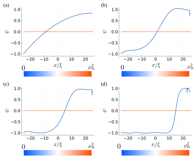
Figure 4: Numerical solutions to the TDGL equation Eq. (III.1) coupled with the spin diffusion equation Eq. (III.1). (a) The given initial state satisfying the boundary conditions Eqs. (42a),  (42b),  (43a) and (43b). (b) - (d) The domain wall moves to the region where the modulus of the spin accumulation is larger.

III.3 Analytical calculation

We consider a flux flow state where the domain wall slowly moves with a constant velocity $v$. We start from the linearization of the variables and equations with respect to $v$. There is no change in the result for the order parameter from Eq. (II.3.1). We expand $\mu^{2}(x,t)$ as

$$\begin{split}\mu^{2}(x,t)&=\mu^{2}_{0}(x-vt)+\mu^{2}_{1}(x)+\mathcal{O}(v^{2})\end{split}$$

$$=\mu^{2}_{1}(x)+\mathcal{O}(v^{2}).$$ (44)

No term in the $0$th order appears since there is no spin accumulation in equilibrium.

III.3.1 linearization with respect to $v$

After the same procedure explained in Sec. II.3, the TDGL equation and the spin diffusion equation are respectively linearized as

$${-\xi^{2}\frac{\partial}{\partial x}\left[\frac{\text{d}\psi_{0}(x)}{\text{d}x}\frac{\partial\phi_{1}(x,t)}{\partial x}-\frac{\text{d}^{2}\psi_{0}(x)}{\text{d}x^{2}}\phi_{1}(x,t)\right]}$$

$$-\tilde{\gamma}v\left(\frac{\text{d}\psi_{0}(x)}{\text{d}x}\right)^{2}-\frac{b}{2}\mu^{2}_{1}(x)\frac{\text{d}}{\text{d}x}\psi^{2}_{0}(x)=0$$ (45)

and

$${\frac{\text{d}}{\text{d}x}\left[\sigma_{0}(x)\frac{\text{d}\mu^{2}_{1}(x)}{\text{d}x}\right]-\frac{\sigma_{0}(x)}{2\mu^{2}_{1}(x)}\left(\frac{\text{d}\mu^{2}_{1}(x)}{\text{d}x}\right)^{2}}$$

$$\frac{2\mu^{2}_{1}(x)}{\tau_{0}(x)}=0,$$ (46)

where the following notations are introduced:

$$b\equiv\frac{T}{T_{\textrm{c}}\left(0\right)\left(T_{\textrm{c}}\left(0\right)-T\right)}\left.\frac{\text{d}T_{\textrm{c}}\left(\mu^{2}\right)}{\text{d}\mu^{2}}\right|_{\mu^{2}=0},$$ (47)

$$\begin{cases}\sigma_{0}(x)\equiv\sigma_{\textrm{n}}+\left(\sigma_{\textrm{s}}-\sigma_{\textrm{n}}\right)\psi_{0}^{2}(x)\\ \tau_{0}(x)\equiv\tau_{\textrm{n}}+\left(\tau_{\textrm{s}}-\tau_{\textrm{n}}\right)\psi_{0}^{2}(x).\end{cases}$$ (48)

Equation (III.3.1) also can be read as the local momentum balance relation. The first and second terms are identical to the ones in Eq. (II.3.2). The third term has $\mu_{1}^{2}(x)$ so that this term provides a force due to the spin density gradient.

III.3.2 forces on domain wall

Forces on the domain wall can be classified into three types based on their origins. The definition of $F_{\textrm{vis}}$ does not require any corrections to Eq. (25). As for the driving force, we define it as

$$\begin{split}F_{\textrm{drv}}&\equiv-\xi^{2}\int_{x_{\textrm{L}}}^{x_{\textrm{R}}}\text{d}x \;\frac{\partial}{\partial x}\left[\frac{\text{d}\psi_{0}(x)}{\text{d}x}\frac{\partial\phi_{1}(x,t)}{\partial x}\right.\\ &\left.\hskip 54.06006pt-\frac{\text{d}^{2}\psi_{0}(x)}{\text{d}x^{2}}\phi_{1}(x,t)\right]\end{split}$$

$$\simeq\xi^{2}\left.\frac{\text{d}^{2}\psi_{0}(x)}{\text{d}x^{2}}\right|_{x=x_{\textrm{R}}}\sqrt{\frac{T_{\textrm{c}}\left(0\right)}{T_{\textrm{c}}\left(0\right)-T}}$$

$$\times\left.\frac{\text{d}}{\text{d}\mu^{2}}\left[\sqrt{\frac{T_{\textrm{c}}\left(\mu^{2}\right)-T}{T_{\textrm{c}}\left(\mu^{2}\right)}}\right]\right|_{\mu^{2}=0}\mu^{2}_{\textrm{R}}$$

$$={\frac{b\xi^{2}}{2}\left.\frac{\text{d}^{2}\psi_{0}(x)}{\text{d}x^{2}}\right|_{x=x_{\textrm{R}}}\mu^{2}_{\textrm{R}}}.$$ (49)

Here, the higher orders of $\mu_{\textrm{R}}^{2}$ are neglected. Both $b$ and $\left.\frac{\text{d}^{2}\psi_{0}(x)}{\text{d}x^{2}}\right|_{x=x_{\textrm{R}}}$ are positive, and so is $F_{\textrm{drv}}>0$, which shows $F_{\textrm{drv}}$ is directed to the boundary with the finite spin accumulation.

The force due to the spin accumulation gradient is defined as

$$\begin{split}F_{\textrm{spin}}&\equiv-\frac{b}{2}\int_{x_{\textrm{L}}}^{x_{\textrm{R}}}\text{d}x \;\mu^{2}_{1}(x)\frac{\text{d}}{\text{d}x}\psi^{2}_{0}(x)\\ &=-\frac{b}{2}\bigg{(}\psi^{2}_{0}(x_{\textrm{R}})\mu^{2}_{1}(x_{\textrm{R}})\\ &-\int_{x_{\textrm{L}}}^{x_{\textrm{R}}}\text{d}x \;\psi^{2}_{0}(x)\frac{\text{d}\mu^{2}_{1}(x)}{\text{d}x}\bigg{)}\\ &=-\frac{b}{2}\bigg{(}\int_{x_{\textrm{L}}}^{x_{\textrm{R}}}\text{d}x \;\psi^{2}_{0}(x_{\textrm{R}})\frac{\text{d}\mu^{2}_{1}(x)}{\text{d}x}\\ &-\int_{x_{\textrm{L}}}^{x_{\textrm{R}}}\text{d}x \;\psi^{2}_{0}(x)\frac{\text{d}\mu^{2}_{1}(x)}{\text{d}x}\bigg{)}\end{split}$$

$$=-\frac{b}{2}\int_{x_{\textrm{L}}}^{x_{\textrm{R}}}\text{d}x \;\left(\psi^{2}_{0}(x_{\textrm{R}})-\psi^{2}_{0}(x)\right)\frac{\text{d}\mu^{2}_{1}(x)}{\text{d}x}.$$ (50)

The factor $\psi^{2}_{0}(x_{\textrm{R}})-\psi^{2}_{0}(x)$ in the integrand of Eq. (III.3.2) makes the force density concentrated around the domain wall. Therefore, it can be regarded as a physically meaningful force acting on the domain wall.

It is essential to evaluate the signs of $\frac{\text{d}\mu^{2}_{1}(x)}{\text{d}x}$ to obtain the sign (direction) of the force. We can easily prove the inequality

$$0\leq\frac{\text{d}\mu^{2}_{1}(x)}{\text{d}x},$$ (51)

which means $\mu^{2}_{1}(x)$ is a monotonically increasing function with respect to $x$. See Appendix C for the proof. For this reason, we have $F_{\textrm{spin}}>0$.

Now, we are ready to determine the sign of the velocity, namely the direction of the motion of the domain wall. From the force-balance relation

$$F_{\textrm{drv}}+F_{\textrm{vis}}+F_{\textrm{spin}}=0,$$ (52)

and the fact that both $F_{\textrm{drv}}$ and $F_{\textrm{spin}}$ are positive, it follows that $F_{\textrm{vis}}<0$. Because of Eq. (25), the signs of the viscous force and the velocity are the opposite, $v>0$. In other words, the domain wall moves toward the region where the modulus of the spin accumulation is larger.

III.4 Remarks

We considered systems with a temperature gradient and a spin accumulation gradient, and found that these two cases can be understood in a similar way. In both cases, the domain wall moves toward the region of the smaller amplitude of the order parameter, namely higher temperature or larger absolute value of spin accumulation.

We note the spin current $j_{\textrm{spin}}$ is not a convenient quantity to describe the phenomena. The ordinary definition of the one-dimantional spin current is given by

$$j_{\textrm{spin}}(x,t)\equiv-\sigma(x,t)\frac{\partial\mu(x,t)}{\partial x}.$$ (53)

When only the sign of $\mu(x,t)$ is changed ($\mu\rightarrow-\mu$), the spin current defined above also is directed to the opposite. However, in our model, what is required as the boundary condition at $x=x_{\textrm{R}}$ is $\mu_{\textrm{R}}^{2}$ due to the spin accumulation-dependency of the critical temperature, and it is not necessary to determine the sign of $\mu_{\textrm{R}}$ itself. This guarantees that the sign of the spin accumulation is not an essential factor for the direction of the motion of the domain wall. In this sense, therefore, we can conclude that the spin current defined by Eq. (53) does not interact with the domain wall, rather the gradient of $\mu^{2}$ is more essential.

IV discussion

We discuss the applicability and prospects of our analysis, which are summarised in the following three points:

1. Our original interest has been in motion of vortices. Nevertheless, the reason for discussing domain walls in this paper was to make the problem more mathematically easier to deal with, and thanks to this, we have successfully obtained analytical expressions such as Eq. (32). The results based on this work can again be recognised as a prototype which provides a theoretical basis to reconsider the motion of vortices under a temperature gradient or spin density gradient.

2. A particularly important field for further application is spintronics in superconductors. Among these, the vortex spin Hall effect, which was recently examined in [41, 42, 44, 45], provides certain evidence of the important role of moving vortices in the spin transport in superconductors. These studies have been carried out under a higher magnetic field region and thus can be regarded as complementary to this work.

3. On the other hand, we can also consider the significance of addressing the domain wall problem instead of vortices. This is the periodic structure of the order parameter in the real space in the Fulde-Ferrell-Larkin-Ovchinnikov (FFLO) state [46, 47]. Here, the Cooper pairs with finite center-of-mass momentum are formed and the periodic structure corresponding to their momentum appears in the real space. In other words, this can be treated as a series of domain walls corresponding to a periodic extension of the system discussed in this study. In fact, the FFLO state that might be realised in zero magnetic field have recently been proposed [48], and dynamics of these states under homogeneous temperature or spin density gradient is an important extension in future.

V conclusion

We studied the dynamics of domain walls in type-II superconductors under the influence of a temperature or a spin accumulation gradient. The time-dependent Ginzburg-Landau equation, which has been widely known to be an effective model for the motion of vortices in the flux flow state under a transport current, and the thermal/spin diffusion equation, whose coefficients vary spatially and temporally depending on the order parameter, were solved. The numerical and analytical results indicate that the domain wall moves toward the hotter boundary in the case of the temperature gradient, and toward the region with the larger magnitude of the spin accumulation in the case of the spin accumulation gradient. These findings from the two different cases are consistently understood as the consequence of the minimization of loss of the condensation energy.

Appendix A Profiles of $\psi_{0}(x)$

From Eq. (II.1.1), the equilibrium Ginzburug-Landau equation is given as

$$-\xi^{2}\frac{\text{d}^{2}\psi(x)}{\text{d}x^{2}}-\psi(x)+\psi^{3}(x)=0.$$ (54)

If $x_{\textrm{R}}=\infty$ and the boundary conditions $\psi(\pm\infty)=\pm 1$ are imposed, the exact solution of the differential equation is given by

$$\psi(x)=\tanh\left(\frac{x}{\sqrt{2}\xi}\right).$$ (55)

However, our target is a finite system, thus some modifications are necessary. To obtain an explicit expression of the exact solution, we assume the solution is odd and holds the boundary conditions

$$\left.\frac{\text{d}\psi(x)}{\text{d}x}\right|_{x=x_{\textrm{L}}}=\left.\frac{\text{d}\psi(x)}{\text{d}x}\right|_{x=x_{\textrm{R}}}=0.$$ (56)

Let $\psi_{0}(x)$ be the odd solution to Eq. (54) under the boundary conditions Eq. (56). Then $\psi_{0}(x)$ can be written as

$$\psi_{0}(x)=\sqrt{1-c}\;\textrm{sn}\left(\sqrt{\frac{1+c}{2}}x,\frac{1-c}{1+c}\right),$$ (57)

where a constant $c$ satisfies

$$\textrm{cn}\left(\sqrt{\frac{1+c}{2}}x_{\textrm{R}},\frac{1-c}{1+c}\right)=0,$$ (58)

and the functions sn, cn are the Jacobi’s elliptic functions. $\psi_{0}(x)$ defined here is a monotonically increasing function which satisfies

$$\left.\frac{\text{d}^{2}\psi(x)}{\text{d}x^{2}}\right|_{x=x_{\textrm{L}}}=-\left.\frac{\text{d}^{2}\psi(x)}{\text{d}x^{2}}\right|_{x=x_{\textrm{R}}}$$ (59)

since it is an odd function.

If $c\rightarrow 0$, then $x_{\textrm{R}}\rightarrow\infty$ and the solution of the Ginzburg-Landau equation approaches $\tanh\left(\frac{x}{\sqrt{2}\xi}\right)$. This is consistent with the well-known result Eq. (55).

Appendix B Derivation of Eq. (II.3.2)

Taking the derivative of both sides of Eq. (54), we find

$$-\xi^{2}\frac{\text{d}^{3}\psi_{0}(x)}{\text{d}x^{3}}-\frac{\text{d}\psi_{0}(x)}{\text{d}x}+3\psi_{0}^{2}(x)\frac{\text{d}\psi_{0}(x)}{\text{d}x}=0.$$ (60)

This is identical to the following expression in terms of the linear operator $\hat{L}\equiv-\xi^{2}\frac{\partial^{2}}{\partial x^{2}}-1+3\psi_{0}^{2}(x)$:

$$\hat{L}\frac{\text{d}\psi_{0}(x)}{\text{d}x}=0.$$ (61)

The similar conditions can be found in the previous studies [11, 12, 17]. In fact, especially in [12], the corresponding condition is called the solvability condition of the inhomogeneous linear differential equations (See Eq. (17)).

For arbitrary differentiable functions $f(x)$ and $g(x)$, we have an identity:

$${\frac{\text{d}}{\text{d}x}\left[f(x)\frac{\text{d}}{\text{d}x}g(x)-g(x)\frac{\text{d}}{\text{d}x}f(x)\right]}$$

$$=f(x)\frac{\text{d}^{2}}{\text{d}x^{2}}g(x)-g(x)\frac{\text{d}^{2}}{\text{d}x^{2}}f(x).$$ (62)

This leads to

$${\frac{\text{d}\psi_{0}(x)}{\text{d}x}\hat{L}\phi_{1}(x,t)=\phi_{1}(x,t)\underset{=0}{\underline{\hat{L}\frac{\text{d}\psi_{0}(x)}{\text{d}x}}}}$$

$$-\xi^{2}\frac{\partial}{\partial x}\left[\frac{\text{d}\psi_{0}(x)}{\text{d}x}\frac{\partial\phi_{1}(x,t)}{\partial x}-\frac{\text{d}^{2}\psi_{0}(x)}{\text{d}x^{2}}\phi_{1}(x,t)\right],$$ (63)

which yields Eq. (II.3.2) when it is combined with Eq. (17). Equation (II.3.2) also can be derived starting from Eq. (15) in [16] which is called ‘the local balance of the force density’ extracting only the $x$-components and omitting electromagnetic quantities.

Appendix C Proof of the inequality (51)

Fron Eq. (III.1), The inequality

$${\frac{\text{d}}{\text{d}x}\left[\sigma_{0}(x)\frac{\text{d}\mu^{2}_{1}(x)}{\text{d}x}\right]}$$

$$=\frac{\sigma_{0}(x)}{2\mu^{2}_{1}(x)}\left(\frac{\text{d}\mu^{2}_{1}(x)}{\text{d}x}\right)^{2}+\frac{2\mu^{2}_{1}(x)}{\tau_{0}(x)}>0$$ (64)

holds. This leads to

$$\frac{\sigma_{0}(x_{\textrm{L}})}{\sigma_{0}(x)}\left.\frac{\text{d}\mu^{2}_{1}(x)}{\text{d}x}\right|_{x=x_{\textrm{L}}}\leq\frac{d\mu^{2}_{1}(x)}{\text{d}x}$$ (65)

for any $x$ in the system. Taking into account $\mu^{2}_{1}(x)\geq 0$ and $\mu^{2}_{1}(x_{\textrm{L}})=0$, we obtain the inequality (51).

References

- Berezinsky [1971] V. L. Berezinsky, Sov. Phys. JETP 32, 493 (1971).
- Berezinsky [1972] V. L. Berezinsky, Sov. Phys. JETP 34, 610 (1972).
- Kosterlitz and Thouless [1973] J. M. Kosterlitz and D. J. Thouless, J. Phys. C: Solid State Phys. 6, 1181 (1973).
- Nagaosa and Tokura [2013] N. Nagaosa and Y. Tokura, Nat. Nanotechnol. 8, 899 (2013).
- Gorter [1962] C. Gorter, Phys. Lett. 1, 69 (1962).
- De Gennes and Matricon [1964] P. G. De Gennes and J. Matricon, Rev. Mod. Phys. 36, 45 (1964).
- Strnad et al. [1964] A. Strnad, C. Hempstead, and Y. Kim, Phys. Rev. Lett. 13, 794 (1964).
- Kim et al. [1965] Y. Kim, C. Hempstead, and A. Strnad, Phys. Rev. 139, A1163 (1965).
- Schmid [1966] A. Schmid, Phys. Kondens. Mater. 5, 302 (1966).
- Gorkov and Kopnin [1971] L. Gorkov and N. Kopnin, Sov. Phys. JETP 33, 1251 (1971).
- Gor’kov and Kopnin [1975] L. P. Gor’kov and N. B. Kopnin, Sov. Phys. Usp. 18, 496 (1975).
- Dorsey [1992] A. T. Dorsey, Phys. Rev. B 46, 8376 (1992).
- Chen et al. [1998] D.-X. Chen, J. J. Moreno, A. Hernando, A. Sanchez, and B.-Z. Li, Phys. Rev. B 57, 5059 (1998).
- Narayan [2003] O. Narayan, J. Phys. A: Math. Gen. 36, L373 (2003).
- Chen et al. [2010] D.-X. Chen, E. Pardo, and A. Sanchez, Physica C 470, 444 (2010).
- Kato and Chung [2016] Y. Kato and C.-K. Chung, J. Phys. Soc. Jpn. 85, 033703 (2016).
- Sugai et al. [2021] S. Sugai, N. Kurosawa, and Y. Kato, Phys. Rev. B 104, 064516 (2021).
- Nozières and Vinen [1966] P. Nozières and W. Vinen, Philos. Mag.-J. Theor. Exp. Appl. Phys. 14, 667 (1966).
- Ao and Thouless [1993] P. Ao and D. J. Thouless, Phys. Rev. Lett. 70, 2158 (1993).
- Šimánek [1995] E. Šimánek, Phys. Rev. B 52, 10336 (1995).
- Sonin [1997] E. Sonin, Phys. Rev. B 55, 485 (1997).
- Gor’kov and Ãliashberg [1968] L. P. Gor’kov and G. M. Ãliashberg, Sov. Phys. JETP 27, 328 (1968).
- Maki [1965] K. Maki, Phys. Rev. 139, A702 (1965).
- Stephen [1966] M. J. Stephen, Phys. Rev. Lett. 16, 801 (1966).
- Otter and Solomon [1966] F. A. Otter and P. R. Solomon, Phys. Rev. Lett. 16, 681 (1966).
- Huebener [1967] R. Huebener, Solid State Commun. 5, 947 (1967).
- Ohta [1967] T. Ohta, Jpn. J. Appl. Phys. 6, 645 (1967).
- Yntema [1967] G. Yntema, Phys. Rev. Lett. 18, 642 (1967).
- Solomon and Otter Jr [1967] P. Solomon and F. Otter Jr, Phys. Rev. 164, 608 (1967).
- Solomon [1968] P. Solomon, Phys. Lett. A 26, 293 (1968).
- Maki [1969] K. Maki, J. Low Temp. Phys. 1, 45 (1969).
- Huebener and Seher [1969] R. P. Huebener and A. Seher, Phys. Rev. 181, 701 (1969).
- de Lange [1974] O. L. de Lange, J. Phys. F 4, 1222 (1974).
- Sergeev et al. [2010] A. Sergeev, M. Reizer, and V. Mitin, Europhys. Lett. 92, 27003 (2010).
- Veshchunov et al. [2016] I. S. Veshchunov, W. Magrini, S. V. Mironov, A. G. Godin, J.-B. Trebbia, A. I. Buzdin, P. Tamarat, and B. Lounis, Nat. Commun. 7, 12801 (2016).
- Duarte et al. [2019] E. C. S. Duarte, A. Presotto, D. Okimoto, V. S. Souto, E. Sardella, and R. Zadorosny, J. Phys.: Condens. Matter 31, 405901 (2019).
- de Toledo et al. [2021] L. V. de Toledo, A. Presotto, L. R. Cadorim, D. Filenga, R. Zadorosny, and E. Sardella, Phys. Lett. A 406, 127449 (2021).
- Takahashi et al. [1999] S. Takahashi, H. Imamura, and S. Maekawa, Phys. Rev. Lett. 82, 3911 (1999).
- Yang et al. [2010] H. Yang, S.-H. Yang, S. Takahashi, S. Maekawa, and S. S. P. Parkin, Nat. Mater. 9, 586 (2010).
- Taira et al. [2018] T. Taira, M. Ichioka, S. Takei, and H. Adachi, Phys. Rev. B 98 (2018).
- Kim et al. [2018] S. K. Kim, R. Myers, and Y. Tserkovnyak, Phys. Rev. Lett. 121, 187203 (2018).
- Vargunin and Silaev [2019] A. Vargunin and M. Silaev, Sci. Rep. 9, 5914 (2019).
- Vargas and Moura [2020] V. Vargas and A. Moura, J. Magn. Magn. Mater 494, 165813 (2020).
- Taira et al. [2021] T. Taira, Y. Kato, M. Ichioka, and H. Adachi, Phys. Rev. B 103, 134417 (2021).
- Adachi et al. [2024] H. Adachi, Y. Kato, J.-i. Ohe, and M. Ichioka, Phys. Rev. B 109, 174503 (2024).
- Fulde and Ferrell [1964] P. Fulde and R. A. Ferrell, Phys. Rev. 135, A550 (1964).
- Larkin and Ovchinnikov [1964] A. I. Larkin and Y. N. Ovchinnikov, Zh. Eksp. Teor. Fiz. 47, 1136 (1964).
- Sumita et al. [2023] S. Sumita, M. Naka, and H. Seo, Phys. Rev. Res. 5, 043171 (2023).