Searching for the QCD critical endpoint using multi-point Padé approximations
Abstract
Using the multi-point Padé approach, we locate Lee-Yang edge singularities of the QCD pressure in the complex baryon chemical potential plane. These singularities are extracted from singularities in the net baryon-number density calculated in lattice QCD at physical quark mass and purely imaginary chemical potential. Taking an appropriate scaling ansatz in the vicinity of the conjectured QCD critical endpoint, we extrapolate the singularities on lattices to pure real baryon chemical potential to estimate the position of the critical endpoint (CEP). We find MeV and MeV, which compares well with recent estimates in the literature. For the slope of the transition line at the critical point we find .
pacs:
11.10.Wx, 11.15.Ha, 12.38.Aw, 12.38.Gc, 12.38.Mh, 24.60.Ky, 25.75.Gz, 25.75.NqIntroduction.—A central goal of the experimental program at the Relativistic Heavy-Ion Collider (RHIC) of Brookhaven National Laboratory (BNL) in the US and at the Large Hadron Collider (LHC) at CERN, Switzerland is the exploration of the phase diagram of quarks and gluons in the plane of temperature and baryon chemical potential as described by the theory of the strong interaction, quantum chromodynamics (QCD). At low and , QCD matter is known to exist as a gas of hadrons. At high and/or , hadrons start to melt and quark-gluon plasma (QGP) is created. The QGP created at high may experience a sharp first-order phase transition as it cools, with bubbles of QGP and hadrons coexisting at a well-defined temperature. The coexistence region ends in a critical point (CEP), where QGP and hadronic matter become indistinguishable. The conjectured CEP belongs to the 3-, universality class.
Progress in understanding the phase diagram at from first-principle lattice QCD calculations, in particular locating the CEP, is stymied by the infamous sign problem. In spite of this difficulty, lattice calculations are able to provide some controlled information of the diagram at sufficiently small . This is accomplished using various techniques, for instance reweighting [1, 2], analytic continuation from purely imaginary [3, 4], and Taylor expansion in [5, 6]. The Taylor expansion technique, while highly successful, is severely limited by the computational power required to compute higher-order Taylor coefficients, with state-of-the-art calculations achieving eighth order [7, 8]. In response to this challenge, various resummation schemes have been proposed [9, 10, 11], which all attempt to probe deeper into the phase diagram without having to compute even higher-order cumulants. Recently the STAR collaboration has found tantalizing evidence of the hint of a QCD critical point [12] in the net proton fluctuation data. However, from the analysis of the QCD equation of state [13, 14] using Taylor expansion and Padé approximation, it is concluded that the CEP is likely not located in the energy range of the beam energy scan II (BESII) program at RHIC in collider mode.
In this paper we adopt the multi-point-Padé resummation method introduced in [15]. The method uses information from simulations at purely imaginary to construct a Padé approximation to the logarithm of the QCD grand partition function for complex . We then determine singularities of the approximant to estimate the CEP location. In particular we consider temperature-like and magnetization-like couplings and near the CEP. Then according to the Lee-Yang theorem [16] applied to the universal theory (3- ), at , zeroes of in the complex -plane that approach the real axis in the thermodynamic limit correspond to phase transitions. For , the closest singularities to the origin are the Lee-Yang edges (LYE). We extrapolate the position of the singularity to the the CEP by following LYE scaling [17].
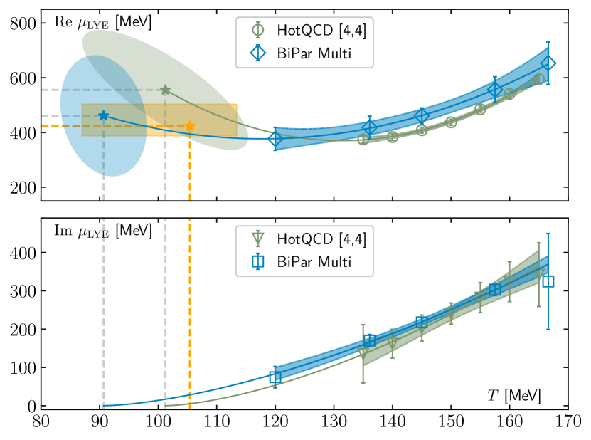
From model calculations and model-independent symmetry arguments we understood that the location of has to be searched below the chiral transition temperature MeV [18]. Thus, we extend our calculations down to MeV in this paper. Our final results are summarized in Fig. 1. We note that they are consistent with the bounds on and mentioned above.
Lattice simulation details.—We generated configurations for a lattice with and and dynamical highly improved staggered quarks (HISQ) [19] using the SIMULATeQCD [20, 21] implementation of the rational hybrid Monte Carlo algorithm (RHMC) [22]. We choose bare parameters along the line of constant physical pion mass obtained for the ratio of light to strange quark mass in Refs. [23, 24, 25]. The simulations run at pure imaginary in the range to avoid the sign problem. For simplicity we set light and strange quark chemical potentials to equal values, , which corresponds to baryon chemical potential and zero strangeness chemical potential . A number of configurations ranging from to was generated for a set of five temperatures ( and MeV) extending far below the chiral transition temperature as summarized in Table 1. The configurations are separated by 10 molecular dynamic time units (MDTU).
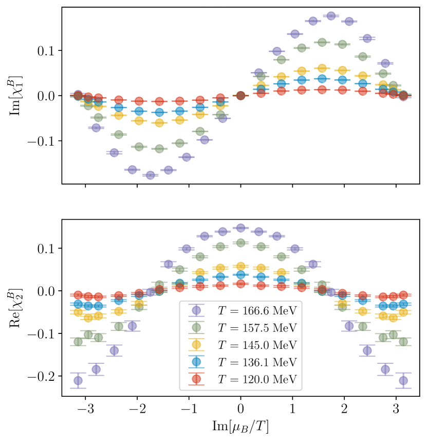
We measured the first- and second-order cumulants of the net baryon-number density, defined as
| (1) |
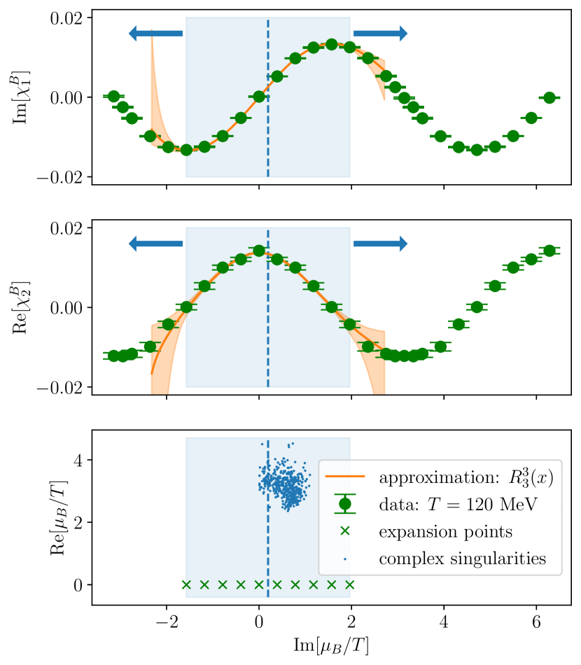
A total of 500 random vectors were used to construct unbiased noisy estimators of the observables. Numerical results are illustrated in Fig. 2. The first-order cumulant is a pure imaginary, odd, and -periodic function of whose signal gets damped as the temperature is decreased. Conversely the second-order cumulant is a pure real, even, and -periodic function of .
| [MeV] | |||
|---|---|---|---|
| 6.170 | 166.6 | 10 | 1800 |
| 6.120 | 157.5 | 10 | 4780 |
| 6.038 | 145.0 | 10 | 5300 |
| 5.980 | 136.1 | 10 | 6840 |
| 5.850 | 120.0 | 10 | 24000 |
Mapping Poles of the multi-point Padé to Lee-Yang Edge singularities.—The first order cumulant is approximated by a rational function of the form
| (2) |
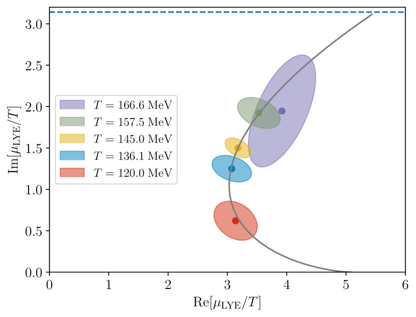
In the generalized least square process [15], data of the first two cumulants are taken into account. The fit interval is contained in , and the length is varied between and . In this way we construct 55 rational approximations per temperature. We obtain the poles of the rational approximation by calculating the roots of the polynomial in the denominator. We keep only the roots in the first quadrant and pick the one which is closest to the center of our fit interval. For each fit interval and temperature we repeat the calculation of poles on samples, generated by bootstrapping over the standard deviation of the cumulant data. In this way we generate distributions of poles which we may represent as 1-confidence ellipses, as shown in Fig. 3 for a particular choice of intervals. We observe that the imaginary part of the poles decreases with decreasing temperature. The large error on the position of the point is likely due to the much lower number of gauge configurations as compared to the other points (see Table 1). The solid grey line in Fig. 3 stems from the fit described below. We note that for MeV, the poles accumulate on the dashed line in Fig. 3 and follow a scaling associated with the Roberge-Weiss transition in QCD [15, 26, 27].
Estimation of CEP location.—The QCD CEP is expected to belong to the 3-, universality class. The mapping from the control parameters and to the temperature-like and magnetization-like scaling directions and of the Ising model is not known. We thus adopt a frequently used linear ansatz for the mapping [28, 29, 30, 31],
| (3) | ||||
with , , and constants , . For the extrapolation of the poles to the real axis, we would like to follow the path of the LYE. Expressed in terms of the scaling variable , it has a constant position [17]
| (4) |
Here , are the well known critical exponents of the 3-, universality class; we use the values , [32]. For a discussion of the universal constant see [33, 34, 35, 36]. Plugging eq. (3) into eq. (4) then implies that should scale [37] as
| (5) | ||||
where the coefficients are functions of the mixing parameters , . In particular we have , which denotes the slope of the transition line at the CEP in the (,)-diagram. Note that the presence of the coefficient goes beyond the linear ansatz of eq. (3) but seems important to extrapolate our current data.
We use eq. (5) to simultaneously fit the real and imaginary parts of our singularities. In total the fit has 5 parameters, , , , , and . We checked that separate fits to real and imaginary parts give very similar results with slightly reduced errors.
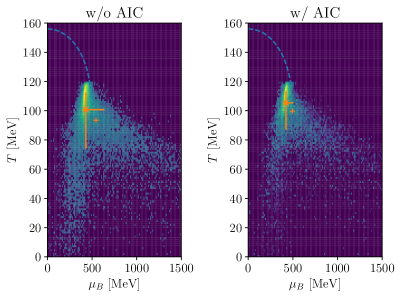
Results for the CEP.—We perform different fits by varying the rational approximation for each temperature, based on different intervals and bootstrapping over the data. The results for the coordinates of the CEP are presented in Fig. 1 as a histogram, weighted with (right) and without (left) the Akaike information criterion (AIC). The median and the 68% confidence interval is estimated and presented in Fig. 1 by star symbols and error bars. In the AIC-weighted case we find
| (6) |
where the errors are statistical errors only. The plus symbols represent the arithmetic mean. Also plotted in Fig. 1 as a blue, dashed line is the crossover temperature. It is interesting to note that the histograms indicate two branches in the tails of the distribution. Whether these branches contain further information on the QCD phase diagram, e.g. on binodal or spinodal lines, will be interesting to discuss in future publications.
In order to compare the results from imaginary chemical potential calculations with the eighth-order Taylor expansion results from [7], the fit with the best (smallest) is presented in Fig. 4 (and Fig. 3). The same fit is applied to the singularities extracted from the [4,4]-Padé resummation of the pressure expansion presented in [7]. The blue and green ellipses drawn in Fig. 4 are the 68%-confidence ellipses obtained from the covariance matrix of the fit parameters. The orange square gives the estimate of the AIC-weighted median over all fits. The error bands on the fit are obtained with error propagation implemented in the AnalysisToolbox [38], which is also used to carry out the fits. Data points and fits of and calculations are compatible within errors; the extrapolated location of the CEP might, however, give rise to some cutoff effects. The fit parameters are summarized in Table 2.
| multi-point Padé | [4,4]-Padé | |||||||||||||||||||||||
| [MeV] | [MeV] | [MeV] | [MeV] | |||||||||||||||||||||
| best fit | 90.7 | 7.7 | 461.2 | 220 | 5.09 | 0.68 | 101 | 15 | 560 | 140 | 5.5 | 1.7 | ||||||||||||
| weight-1 | 105.4 | 8.0 | 18.4 | 422.9 | 80.5 | 34.9 | 3.92 | 1.52 | 0.24 | |||||||||||||||
| weight-2 | 100.8 | 11.6 | 26.8 | 430.9 | 208.2 | 42.2 | 4.20 | 4.13 | 0.47 | |||||||||||||||
| best fit | -6.2 | 9.2 | 0.115 | 0.090 | 0.424 | 0.086 | -12.3 | 8.1 | 0.203 | 0.059 | 0.55 | 0.25 | ||||||||||||
Besides the location of the CEP, we can also estimate the slope of the transition line at the CEP. In the -diagram, the slope is given as . Since the direction of the temperature-like scaling field is tangential to the transition line at the CEP, we can also estimate the angles between the -axis and the axes of the -diagram.
| (7) |
We note that the map in eq. (3) can be decomposed into translation, rotations and scales. In this case one of the above angles enters directly the mapping between the QCD parameter and the scaling fields.
Discussion.—An important consistency check for our results on the CEP location is the comparison with the crossover line. A natural parametrization of the pseudo-critical temperature is given as
| (8) |
where MeV is the crossover temperature at and . In recent lattice QCD and other calculations, continuum extrapolated results for the curvature coefficients and were presented and remarkably agreement was found at least for : (for the case ) [39, 40, 41, 42, 43, 44, 45]. Note that frequently the crossover line is also parametrized with and coefficients , . We can map one parametrization to the other by setting and , with differences remaining at . Our CEP location for is roughly in agreement with the parametrization in . This parametrization is shown in Fig. 1 as dashed line. However, in the region where the CEP is located the contribution of the coefficient would already be significant, i.e. the two parametrizations with and differ substantially for MeV or MeV. Plugging or into the latter, would increase or respectively. We note that current cutoff effects that we observe between and calculations would lead to a continuum result of that is consistent with , which is favored by lattice calculations. Current estimates give (again for ) [39]. More precisely the value of would increase to MeV. The reason why we are not seriously attempting to perform the continuum extrapolation here is that the and calculations differ by their methodology and might suffer from different systematic effects.
Our estimate for the CEP location (at least when taking cutoff effects into account) compares favorably with a number of other results and constraints. To begin with, it ought to lie outside the estimated convergence region of the Taylor series for , i.e. it is expected111Strictly speaking, this estimate of the convergence radius depends on e.g. the temperature. Some of these earlier estimates come from coarse lattices. Still, they indicate convergence in the same general regime. that [46, 47, 48, 7]. Moreover, if the CEP exists, it is expected to occur at a lower temperature than the chiral transition temperature [49], which is known to be MeV [18]. Our estimate conforms to both of these expectations. Additionally it is in rough agreement with recent predictions from Dyson-Schwinger equations [44, 50], the functional renormalization group [43], and black-hole engineering [51]. Similar to our approach, the conformal Padé applied to the same HotQCD data yields a compatible result as well [52].
An important limitation of the estimates presented here222And therefore also for Ref. [52]. is that they are not fully extrapolated to the continuum limit. For the multi-point Padé, we are limited to , and the HotQCD data utilize and on lattices. At this stage, it appears clear that both data sets are sensitive to a non-trivial singularity structure in that is consistent with Lee-Yang edge scaling, but in principle our estimates of the location of are distorted by cutoff effects.
Summary.—Here we present a new strategy for the critical point search at by means of first principle lattice QCD calculations. Based on rational function approximations of the cumulants of the baryon-number fluctuations at imaginary chemical potential we determine singularities in the complex plane. We extrapolate these singularities using a scaling ansatz motivated by the temperature scaling of the Lee-Yang edge singularity. The rational function approximations are obtained by a multi-point Padé analysis on a sliding interval embedded in . For the results we find MeV and MeV, based on different fits. However we expect that cutoff effects will alter towards larger values of around MeV. This estimate is roughly consistent with other estimates in the literature and also with the current determination of the crossover line.
Acknowledgement.—This work was supported by the Deutsche Forschungsgemeinschaft (DFG, German Research Foundation) Proj. No. 315477589-TRR 211, by the PUNCH4NFDI consortium supported by the Deutsche Forschungsgemeinschaft (DFG, German Research Foundation) with project number 460248186 (PUNCH4NFDI) and by INFN (Istituto Nazionale di Fisica Nucleare) under research project i.s. QCDLAT. In its early phase this work also received funding from the European Union’s Horizon 2020 research and innovation programme under the Marie Skłodowska-Curie grant agreement No. 813942 (EuroPLEx). Numerical calculations have been made possible through EuroHPC JU and PRACE grants at CINECA, Italy on Leonardo and Marconi100, and through the Gauss Centre for Supercomputing e.V. (www.gauss-centre.eu) on the GCS Supercomputer JUWELS [53] at Jülich Supercomputing Centre (JSC). Additional calculations have been performed on Leonardo under the INFN-CINECA agreement for HPC and on the GPU clusters at Bielefeld University, Germany. We also acknowledge support of the Bielefeld NPC.NRW team. DAC was supported by the National Science Foundation under Grant PHY20-13064. KZ acknowledges support by the project “Non-perturbative aspects of fundamental interactions, in the Standard Model and beyond” funded by MUR, Progetti di Ricerca di Rilevante Interesse Nazionale (PRIN), Bando 2022, Grant 2022TJFCYB (CUP I53D23001440006).
References
- Barbour et al. [1998] I. M. Barbour, S. E. Morrison, E. G. Klepfish, J. B. Kogut, and M.-P. Lombardo, Results on finite density QCD, Nuclear Physics B - Proceedings Supplements 60, 220 (1998).
- Fodor and Katz [2002] Z. Fodor and S. Katz, A new method to study lattice QCD at finite temperature and chemical potential, Physics Letters B 534, 87 (2002).
- de Forcrand and Philipsen [2002] P. de Forcrand and O. Philipsen, The QCD phase diagram for small densities from imaginary chemical potential, Nucl. Phys. B 642, 290 (2002), arXiv:hep-lat/0205016 .
- D’Elia and Lombardo [2003] M. D’Elia and M.-P. Lombardo, Finite density QCD via imaginary chemical potential, Phys. Rev. D 67, 014505 (2003), arXiv:hep-lat/0209146 .
- Gavai and Gupta [2003] R. V. Gavai and S. Gupta, Pressure and nonlinear susceptibilities in QCD at finite chemical potentials, Phys. Rev. D 68, 034506 (2003), arXiv:hep-lat/0303013 .
- Allton et al. [2005] C. R. Allton, M. Doring, S. Ejiri, S. J. Hands, O. Kaczmarek, F. Karsch, E. Laermann, and K. Redlich, Thermodynamics of two flavor QCD to sixth order in quark chemical potential, Phys. Rev. D 71, 054508 (2005), arXiv:hep-lat/0501030 .
- Bollweg et al. [2022] D. Bollweg, J. Goswami, O. Kaczmarek, F. Karsch, S. Mukherjee, P. Petreczky, C. Schmidt, and P. Scior (HotQCD), Taylor expansions and Padé approximants for cumulants of conserved charge fluctuations at nonvanishing chemical potentials, Phys. Rev. D 105, 074511 (2022), arXiv:2202.09184 [hep-lat] .
- Borsanyi et al. [2018] S. Borsanyi, Z. Fodor, J. N. Guenther, S. K. Katz, K. K. Szabo, A. Pasztor, I. Portillo, and C. Ratti, Higher order fluctuations and correlations of conserved charges from lattice QCD, JHEP 10, 205, arXiv:1805.04445 [hep-lat] .
- Borsányi et al. [2021] S. Borsányi, Z. Fodor, J. N. Guenther, R. Kara, S. D. Katz, P. Parotto, A. Pásztor, C. Ratti, and K. K. Szabó, Lattice QCD equation of state at finite chemical potential from an alternative expansion scheme, Phys. Rev. Lett. 126, 232001 (2021), arXiv:2102.06660 [hep-lat] .
- Mondal et al. [2022] S. Mondal, S. Mukherjee, and P. Hegde, Lattice QCD Equation of State for Nonvanishing Chemical Potential by Resumming Taylor Expansions, Phys. Rev. Lett. 128, 022001 (2022), arXiv:2106.03165 [hep-lat] .
- Mitra et al. [2022] S. Mitra, P. Hegde, and C. Schmidt, New way to resum the lattice QCD Taylor series equation of state at finite chemical potential, Phys. Rev. D 106, 034504 (2022), arXiv:2205.08517 [hep-lat] .
- Adam et al. [2021] J. Adam et al. (STAR), Nonmonotonic Energy Dependence of Net-Proton Number Fluctuations, Phys. Rev. Lett. 126, 092301 (2021), arXiv:2001.02852 [nucl-ex] .
- Bollweg et al. [2023] D. Bollweg, D. A. Clarke, J. Goswami, O. Kaczmarek, F. Karsch, S. Mukherjee, P. Petreczky, C. Schmidt, and S. Sharma (HotQCD), Equation of state and speed of sound of (2+1)-flavor QCD in strangeness-neutral matter at nonvanishing net baryon-number density, Phys. Rev. D 108, 014510 (2023), arXiv:2212.09043 [hep-lat] .
- Goswami [2023] J. Goswami (HotQCD), The isentropic equation of state of (2+1)-flavor QCD: An update based on high precision Taylor expansion and Pade-resummed expansion at finite chemical potentials, PoS LATTICE2022, 149 (2023), arXiv:2212.10016 [hep-lat] .
- Dimopoulos et al. [2022] P. Dimopoulos, L. Dini, F. Di Renzo, J. Goswami, G. Nicotra, C. Schmidt, S. Singh, K. Zambello, and F. Ziesché, Contribution to understanding the phase structure of strong interaction matter: Lee-Yang edge singularities from lattice QCD, Phys. Rev. D 105, 034513 (2022), arXiv:2110.15933 [hep-lat] .
- Yang and Lee [1952] C.-N. Yang and T. D. Lee, Statistical theory of equations of state and phase transitions. 1. Theory of condensation, Phys. Rev. 87, 404 (1952).
- Fisher [1978] M. E. Fisher, Yang-Lee Edge Singularity and Field Theory, Phys. Rev. Lett. 40, 1610 (1978).
- Ding et al. [2019] H. T. Ding et al. (HotQCD), Chiral Phase Transition Temperature in ( 2+1 )-Flavor QCD, Phys. Rev. Lett. 123, 062002 (2019), arXiv:1903.04801 [hep-lat] .
- Follana et al. [2007] E. Follana, Q. Mason, C. Davies, K. Hornbostel, G. P. Lepage, J. Shigemitsu, H. Trottier, and K. Wong (HPQCD, UKQCD), Highly improved staggered quarks on the lattice, with applications to charm physics, Phys. Rev. D 75, 054502 (2007), arXiv:hep-lat/0610092 .
- Altenkort et al. [2022] L. Altenkort, D. Bollweg, D. A. Clarke, O. Kaczmarek, L. Mazur, C. Schmidt, P. Scior, and H.-T. Shu, HotQCD on multi-GPU Systems, PoS LATTICE2021, 196 (2022), arXiv:2111.10354 [hep-lat] .
- Mazur et al. [2024] L. Mazur et al. (HotQCD), SIMULATeQCD: A simple multi-GPU lattice code for QCD calculations, Comput. Phys. Commun. 300, 109164 (2024), arXiv:2306.01098 [hep-lat] .
- Clark and Kennedy [2007] M. A. Clark and A. D. Kennedy, Accelerating dynamical fermion computations using the rational hybrid Monte Carlo (RHMC) algorithm with multiple pseudofermion fields, Phys. Rev. Lett. 98, 051601 (2007), arXiv:hep-lat/0608015 .
- Bazavov et al. [2012] A. Bazavov et al., The chiral and deconfinement aspects of the QCD transition, Phys. Rev. D 85, 054503 (2012), arXiv:1111.1710 [hep-lat] .
- Bazavov et al. [2014] A. Bazavov et al. (HotQCD), Equation of state in ( 2+1 )-flavor QCD, Phys. Rev. D 90, 094503 (2014), arXiv:1407.6387 [hep-lat] .
- Bollweg et al. [2021] D. Bollweg, J. Goswami, O. Kaczmarek, F. Karsch, S. Mukherjee, P. Petreczky, C. Schmidt, and P. Scior (HotQCD), Second order cumulants of conserved charge fluctuations revisited: Vanishing chemical potentials, Phys. Rev. D 104, 074512 (2021), arXiv:2107.10011 [hep-lat] .
- Clarke et al. [2023] D. A. Clarke, K. Zambello, P. Dimopoulos, F. Di Renzo, J. Goswami, G. Nicotra, C. Schmidt, and S. Singh, Determination of Lee-Yang edge singularities in QCD by rational approximations, PoS LATTICE2022, 164 (2023), arXiv:2301.03952 [hep-lat] .
- Schmidt et al. [2024] C. Schmidt, D. A. Clarke, P. Dimopoulos, F. Di Renzo, J. Goswami, S. Singh, V. V. Skokov, and K. Zambello, Universal scaling and the asymptotic behaviour of Fourier coefficients of the baryon-number density in QCD, in 40th International Symposium on Lattice Field Theory (2024) arXiv:2401.07790 [hep-lat] .
- Rehr and Mermin [1973] J. J. Rehr and N. D. Mermin, Revised Scaling Equation of State at the Liquid-Vapor Critical Point, Phys. Rev. A 8, 472 (1973).
- Nonaka and Asakawa [2005] C. Nonaka and M. Asakawa, Hydrodynamical evolution near the QCD critical end point, Phys. Rev. C 71, 044904 (2005), arXiv:nucl-th/0410078 .
- Parotto et al. [2020] P. Parotto, M. Bluhm, D. Mroczek, M. Nahrgang, J. Noronha-Hostler, K. Rajagopal, C. Ratti, T. Schäfer, and M. Stephanov, QCD equation of state matched to lattice data and exhibiting a critical point singularity, Phys. Rev. C 101, 034901 (2020), arXiv:1805.05249 [hep-ph] .
- Kahangirwe et al. [2024] M. Kahangirwe, S. A. Bass, E. Bratkovskaya, J. Jahan, P. Moreau, P. Parotto, D. Price, C. Ratti, O. Soloveva, and M. Stephanov, Finite density QCD equation of state: critical point and lattice-based -expansion, (2024), arXiv:2402.08636 [nucl-th] .
- El-Showk et al. [2014] S. El-Showk, M. F. Paulos, D. Poland, S. Rychkov, D. Simmons-Duffin, and A. Vichi, Solving the 3d Ising Model with the Conformal Bootstrap II. c-Minimization and Precise Critical Exponents, J. Stat. Phys. 157, 869 (2014), arXiv:1403.4545 [hep-th] .
- Connelly et al. [2020] A. Connelly, G. Johnson, F. Rennecke, and V. Skokov, Universal Location of the Yang-Lee Edge Singularity in Theories, Phys. Rev. Lett. 125, 191602 (2020), arXiv:2006.12541 [cond-mat.stat-mech] .
- Rennecke and Skokov [2022] F. Rennecke and V. V. Skokov, Universal location of Yang–Lee edge singularity for a one-component field theory in 1d4, Annals Phys. 444, 169010 (2022), arXiv:2203.16651 [hep-ph] .
- Johnson et al. [2023] G. Johnson, F. Rennecke, and V. V. Skokov, Universal location of Yang-Lee edge singularity in classic O(N) universality classes, Phys. Rev. D 107, 116013 (2023), arXiv:2211.00710 [hep-ph] .
- Karsch et al. [2024] F. Karsch, C. Schmidt, and S. Singh, Lee-Yang and Langer edge singularities from analytic continuation of scaling functions, Phys. Rev. D 109, 014508 (2024), arXiv:2311.13530 [hep-lat] .
- Stephanov [2006] M. A. Stephanov, QCD critical point and complex chemical potential singularities, Phys. Rev. D 73, 094508 (2006), arXiv:hep-lat/0603014 .
- Altenkort et al. [2023] L. Altenkort, D. A. Clarke, J. Goswami, and H. Sandmeyer, Streamlined data analysis in Python, 40th International Symposium on Lattice Field Theory, PoS LATTICE2023, 136 (2023), arXiv:2308.06652 [hep-lat] .
- Bazavov et al. [2019] A. Bazavov et al. (HotQCD), Chiral crossover in QCD at zero and non-zero chemical potentials, Phys. Lett. B 795, 15 (2019), arXiv:1812.08235 [hep-lat] .
- Borsanyi et al. [2020] S. Borsanyi, Z. Fodor, J. N. Guenther, R. Kara, S. D. Katz, P. Parotto, A. Pasztor, C. Ratti, and K. K. Szabo, QCD Crossover at Finite Chemical Potential from Lattice Simulations, Phys. Rev. Lett. 125, 052001 (2020), arXiv:2002.02821 [hep-lat] .
- Bellwied et al. [2015] R. Bellwied, S. Borsanyi, Z. Fodor, J. Günther, S. D. Katz, C. Ratti, and K. K. Szabo, The QCD phase diagram from analytic continuation, Phys. Lett. B 751, 559 (2015), arXiv:1507.07510 [hep-lat] .
- Bonati et al. [2018] C. Bonati, M. D’Elia, F. Negro, F. Sanfilippo, and K. Zambello, Curvature of the pseudocritical line in QCD: Taylor expansion matches analytic continuation, Phys. Rev. D 98, 054510 (2018), arXiv:1805.02960 [hep-lat] .
- Fu et al. [2020] W.-j. Fu, J. M. Pawlowski, and F. Rennecke, QCD phase structure at finite temperature and density, Phys. Rev. D 101, 054032 (2020), arXiv:1909.02991 [hep-ph] .
- Gao and Pawlowski [2021] F. Gao and J. M. Pawlowski, Chiral phase structure and critical end point in QCD, Phys. Lett. B 820, 136584 (2021), arXiv:2010.13705 [hep-ph] .
- Ali et al. [2024] M. S. Ali, D. Biswas, A. Jaiswal, and H. Mishra, Effects of strangeness on the chiral pseudo-critical line, (2024), arXiv:2403.11965 [nucl-th] .
- Giordano and Pásztor [2019] M. Giordano and A. Pásztor, Reliable estimation of the radius of convergence in finite density QCD, Phys. Rev. D 99, 114510 (2019), arXiv:1904.01974 [hep-lat] .
- Giordano et al. [2020] M. Giordano, K. Kapas, S. D. Katz, D. Nogradi, and A. Pasztor, Radius of convergence in lattice QCD at finite with rooted staggered fermions, Phys. Rev. D 101, 074511 (2020), [Erratum: Phys.Rev.D 104, 119901 (2021)], arXiv:1911.00043 [hep-lat] .
- Mukherjee and Skokov [2021] S. Mukherjee and V. Skokov, Universality driven analytic structure of the QCD crossover: radius of convergence in the baryon chemical potential, Phys. Rev. D 103, L071501 (2021), arXiv:1909.04639 [hep-ph] .
- Karsch [2019] F. Karsch, Critical behavior and net-charge fluctuations from lattice QCD, PoS CORFU2018, 163 (2019), arXiv:1905.03936 [hep-lat] .
- Gunkel and Fischer [2021] P. J. Gunkel and C. S. Fischer, Locating the critical endpoint of QCD: Mesonic backcoupling effects, Phys. Rev. D 104, 054022 (2021), arXiv:2106.08356 [hep-ph] .
- Hippert et al. [2023] M. Hippert et al., Bayesian location of the QCD critical point from a holographic perspective, 2309.00579 (2023).
- Basar [2023] G. Basar, On the QCD critical point, Lee-Yang edge singularities and Pade resummations, 2312.06952 (2023).
- Jülich Supercomputing Centre [2021] Jülich Supercomputing Centre, JUWELS Cluster and Booster: Exascale Pathfinder with Modular Supercomputing Architecture at Juelich Supercomputing Centre, Journal of large-scale research facilities 7, 10.17815/jlsrf-7-183 (2021).
supplemental material
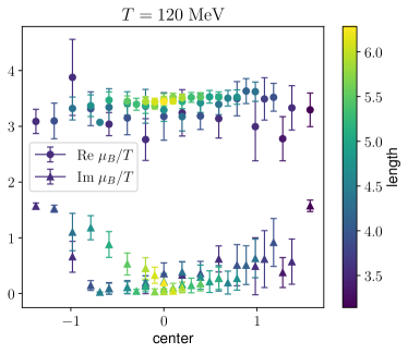
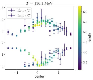
The sliding window analysis of the rational function approximation.–As we had already observed in Ref. [15], there is an interval dependence for the poles located by multi-point Padé analysis. When we change the interval we become more sensitive to some singularities and less to others. In particular we observe that for symmetric intervals centered at , thermal singularities that belong to the Roberge-Weiss transition are favored. For that reason we perform a very general sliding window analysis where we vary the interval length as well as the center of the interval used in the rational approximation. The length is varied between and , whereas the center of the interval is located in [, ]. Note that only the points between and are calculated. In other regions the data is duplicated through reflection symmetry and periodicity. The procedure is visualized in Fig. 5, for the example of the MeV data and can be summarized by the following algorithm:
The subroutine SelectInterval is chosen to be deterministic. We number all possible combinations of interval length and center in the above mentioned ranges that are possible with our data points. We find . The subroutine DrawBootstrapSample on the other hand assumes independent and normal distributed errors on the data points that have support in the interval . The subroutine RationalApproximation performs a combined fit to the and data from the sample . We use the rational function as given in eq. (2). We checked that higher order rational approximations give very similar results, however, the initial set of parameters for these fits have to be chosen more carefully to ensure convergence, and cancellations of poles in the numerator and denominator are more likely to occur. We keep only approximations with . In CalcSingularities , we determine the roots of the denominator of and check if they are canceled by poles in the numerator. For such cancellations we allow for a tolerance of . Finally we calculate the mean and error for the singularities for which we chose the median and 1- percentile of the real and imaginary part. For the ellipses shown in Fig. 3 we also calculate the Pearson correlation coefficient. We repeat the sliding window analysis for each of the temperatures. The results for the real and imaginary parts of the singularities at the example of MeV and MeV are shown in Fig. 6.
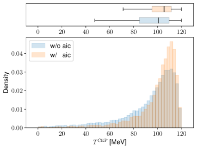
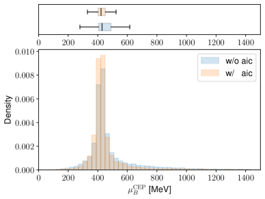
Statistical analysis of fit results.– Next we perform scaling fits to equation (5). We chose one of the 55 intervals for each of the 5 different temperatures. This gives us different data sets. In practice we chose random samples from possible interval combinations. The results for and are summarized in Fig. 1 as a 2d-histogram. We also calculate the relative likelihood of each fit in accordance with the Akaike information criterion. In particular, we calculate the weights
| (9) |
where index labels the fits and . We observe that models with small or large are further suppressed when we weight the results with . A one dimensional histogram of the and results, respectively, is shown in Fig. 7. On top of the histograms we show standard box-and-whiskers diagrams for the data, where the vertical line inside the boxes indicates the median. Note that the size of the box indicates here the interquartile range (IQR=-) and the whiskers have the length of 1.5IQR, except for , where we indicate the maximal values that occur.