PIR: Remote Sensing Image-Text Retrieval with Prior Instruction Representation Learning

Abstract

Remote sensing image-text retrieval constitutes a foundational aspect of remote sensing interpretation tasks, facilitating the alignment of vision and language representations. This paper introduces a prior instruction representation (PIR) learning paradigm that draws on prior knowledge to instruct adaptive learning of vision and text representations. Based on PIR, a domain-adapted remote sensing image-text retrieval framework PIR-ITR is designed to address semantic noise issues in vision-language understanding tasks. However, with massive additional data for pre-training the vision-language foundation model, remote sensing image-text retrieval is further developed into an open-domain retrieval task. Continuing with the above, we propose PIR-CLIP, a domain-specific CLIP-based framework for remote sensing image-text retrieval, to address semantic noise in remote sensing vision-language representations and further improve open-domain retrieval performance. In vision representation, Vision Instruction Representation (VIR) based on Spatial-PAE utilizes the prior-guided knowledge of the remote sensing scene recognition by building a belief matrix to select key features for reducing the impact of semantic noise. In text representation, Language Cycle Attention (LCA) based on Temporal-PAE uses the previous time step to cyclically activate the current time step to enhance text representation capability. A cluster-wise Affiliation Loss (AL) is proposed to constrain the inter-classes and to reduce the semantic confusion zones in the common subspace. Comprehensive experiments demonstrate that PIR could enhance vision and text representations and outperform the state-of-the-art methods of closed-domain and open-domain retrieval on two benchmark datasets, RSICD and RSITMD.

I Introduction

Remote Sensing Image-Text Retrieval (RSITR) aims to use image patches (text) to search for matching text (image patches) from large-scale remote sensing databases collected by satellites or aerial drones to obtain valuable information. Due to its important applications [1, 2, 3, 4, 5]in natural resource exploration and disaster monitoring [6, 7], RSITR has received much attention from researchers. In recent years, the rapid expansion of remote sensing data [8, 9] coupled with advancements in cross-modal retrieval techniques [10, 11, 12, 13, 14, 15, 16] has provided substantial data and technical support for RSITR.

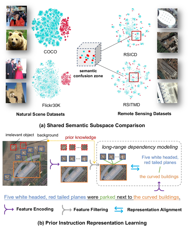
Figure 1: (a): Shared semantic subspace comparison in natural scene datasets COCO and Flickr30K, and remote sensing datasets RSICD and RSITMD, the red squares represent vision embeddings, and the blue circles represent text embeddings; (b): Pipeline of our proposed PIR to reduce the influence of semantic noise.

According to different training paradigms, RSITR can be divided into closed and open-domain retrieval. Closed-domain retrieval is a supervised training and retrieval under a single dataset, but it is less capable of retrieving more complex ground elements. In closed-domain retrieval, most existing methods are CNN-based [17] vision representation and RNN-based [18] text representation using pair-wise triplet loss [19]) for optimization. Abdullah et al. [20] first applied modality fusion to solve the remote sensing image-text matching problem. Lv et al. [21] used knowledge distillation to transform the fusion information of modality to vision and text representation learning. Mi et al. [22] utilized a knowledge graph to enrich text semantics and to reduce the information gap between vision and language. Yuan et al. [23] developed an RSCTIR model to understand multi-level visual semantics based on global and local information. Pan et al. [24] proposed a scene-aware aggregation network to improve the fine-grained perception of the scene. These approaches benefit from a good vision and text representation and perform poorly for long-range dependency modelling [25, 26]. Open-domain retrieval is fine-tuned on a small dataset after pre-training on an additional large-scale dataset with better ground element recognition. CLIP [27] inspired efforts with powerful zero-shot learning on visual interpretation tasks in open-domain retrieval. Subsequently, RemoteCLIP [28], GeoRSCLIP [29], and SkyCLIP [30] models were introduced to establish a foundation vision-language model for remote sensing (RSVLM) and improve large-scale open-domain image-text retrieval performance. Their objective is to establish a foundation RSVLM rather than delving into methods to enhance the visual representation of remote sensing.

Figure 1(a) visualizes the subspaces on the natural scene datasets COCO [31] and Flickr30K [32], and remote sensing datasets RSICD [8] and RSITMD [9] using t-SNE [33]. In the natural scene subspace, image and text representations are separated more significantly than in the remote sensing subspace. Unlike natural images, small-scale objects in remote sensing images are more prone to the interference of semantic noise [23], such as background, irrelevant objects, etc. Excessive attention to semantic noise biases the vision and text representations and causes semantic confusion zones [24] (vision embeddings and text embeddings crossover zones), which greatly affects retrieval performance. Yuan et al. [9] used a redundant feature filtering network to filter useless features. Pan et al. [24] proposed a scene-aware aggregation network to reduce the semantic confusion zones in the common subspace. Nevertheless, these methods are based on CNN-based vision representation and RNN-based text representation, which is not effective for long-range dependency modeling [34] and the growth of remote sensing data. With the powerful performance of Transformer in computer vision [35] and natural language processing [36], Transformer-based vision and text representations enable retrieval performance to be further improved. Zhang et al. [37] designed a decoupling module based on Transformer to obtain invariant features in the modalities. However, this method ignores the remote sensing data characteristics [23, 24], making limited improvement in retrieval performance. In short, a framework specific to remote sensing data becomes necessary.

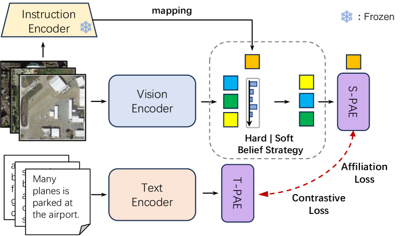
Figure 2: Overview of our proposed PIR-ITR, with two progressive attention encoders (PAE), including Spatial-PAE and Temporal-PAE, as the base template to construct Vision Instruction Representation and Language Cycle Attention for unbiased representation and utilize contrastive loss and attribution loss to optimize vision and text representations in the common subspace. S-PAE and T-PAE represent Spatial-PAE and Temporal-PAE, respectively.

We propose a Prior Instruction Representation (PIR) to reduce the influence of semantic noise as shown in Figure 1(b). Firstly, PIR-ITR is designed to utilize prior knowledge of remote sensing scene recognition [38] to perform long-range dependency modelling, ensuring the unbiased vision and text representations, as shown in Figure 2. Two progressive attention encoder (PAE) structures, Spatial-PAE and Temporal-PAE, are proposed to perform long-range dependency modelling to enhance key feature representation. Spatial-PAE utilizes external knowledge to enhance visual-spatial perception. Temporal-PAE is applied to reduce the inaccuracy of position information by leveraging the previous time step to activate the current time step cyclically. In vision representation, a Vision Instruction Representation (VIR) based on Spatial-PAE is proposed to filter features by building a belief matrix, aiming for an unbiased vision representation. In text representation, we design a Language Cycle Attention (LCA) based on Temporal-PAE to obtain an unbiased text representation. For the inter-class similarity [9] in the remote sensing data domain, a cluster-wise attribution loss is proposed to constrain the inter-classes and reduce the semantic confusion zones in the common subspace. Extensive experiments are conducted on two benchmark datasets, RSICD [8], and RSITMD [9], to demonstrate the effectiveness of our approach, resulting in improvements of 4.9% and 4.0% on the RSICD and RSITMD respectively. Based on the PIR, we propose a two-stage CLIP-based method, PIR-CLIP, to address semantic noise in remote sensing vision-language representations and improve open-domain image-text retrieval further. Unlike vanilla CLIP structure, visual prior knowledge is used to instruct visual representations, as shown in Figure 3. It has a universal model architecture and higher retrieval performance than PIR-ITR, which adjusts the visual representation through instruction embeddings and only needs to fine-tune a few parameters, with 7.3% and 9.4% improvement over open-domain state-of-the-art methods on RSICD dataset and RSITMD dataset, respectively.

Our key contributions are as follows:

• We propose a prior instruction representation (PIR) learning paradigm, which utilizes prior knowledge of the remote sensing scene recognition for unbiased representation to enhance vision-language understanding, which can be applied to closed-domain and open-domain retrieval.

• PIR-ITR is proposed for closed-domain retrieval. Two PAE structures, Spatial-PAE and Temporal-PAE, are proposed to perform long-range dependency modelling to enhance key feature representation. VIR based on Spatial-PAE uses instruction embedding to filter features by building a belief matrix aiming for an unbiased vision representation. LCA based on Temporal-PAE improves text representation by using the previous time step to activate the current time step.

• PIR-CLIP, a two-stage CLIP-based method with prior instruction representation learning, is proposed to address semantic noise in remote sensing vision-language representations and improve open-domain retrieval performance further. First, the image and text encoders are pre-trained on five million coarse-grained remote sensing image-text pairs, and then vision instruction fine-tuning is performed on fine-grained remote sensing image-text pairs.

• A cluster-wise attribution loss is proposed to constrain the inter-classes and reduce the semantic confusion zones in the common subspace.

Compared with our previous work [39], we further extend the PIR learning paradigm to open-domain retrieval based on the former closed-domain retrieval. This work designs PIR-ITR with a soft belief strategy to tune visual representation dynamically and proposes PIR-CLIP based on PIR, which address semantic noise in remote sensing vision-language representations and further improves the remote sensing image-text retrieval performance, especially in open-domain retrieval performance, as well as adds more detailed experiments to validate the effectiveness of our method.

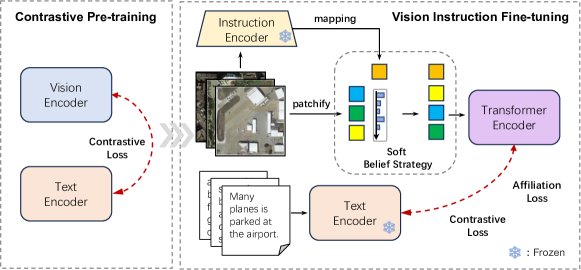
Figure 3: PIR-CLIP framework, a two-stage strategy to pre-train vision encoder and text encoder on large-scale remote sensing image-text pairs, then perform vision instruction fine-tuning on a remote sensing image-text retrieval datasets for open-domain retrieval, which adjusts the visual representation through instruction embeddings and only needs to fine-tune a few parameters.

II RELATED WORK

II-A Remote Sensing Image-text Retrieval

Although traditional cross-modal retrieval methods based on natural images are increasingly mature, these methods cannot be directly applied to multiscale and redundant remote sensing images. There is still a long way to go in remote sensing cross-modal retrieval. According to different training paradigms, the remote sensing cross-modal retrieval methods can be divided into two categories: closed-domain and open-domain methods.

Closed-domain method is a supervised method for training and retrieval under a single dataset, but it is less capable of retrieving more complex ground elements. Some works [40, 20, 22, 23, 37] only perform self-interaction on the same modality to obtain an enhanced modal semantic representation. [40, 20] used the information of different modalities to obtain a joint semantic representation. Might et al. [22] proposed a knowledge-based method to solve the problem of coarse-grained textual descriptions. Yuan et al. [23] proposed a network structure based on global and local information, using attention-based modules to fuse multi-level information dynamically. Zhang et al. [37] designed a reconstruction module to reconstruct the decoupled features, which ensures the maximum retention of information in the features. Some others [21, 41, 42, 9] use information between different attention mechanisms or shared parameter networks for interactive learning. Lv et al. [21] propose a fusion-based association learning model to fuse image and text information across modalities to improve the semantic relevance of different modalities. Particularly, Yuan et al. [41] used a shared pattern transfer module to realize the interaction between modalities, solving the semantic heterogeneity problem between different modal data. Cheng et al. [42] propose a semantic alignment module that uses an attention mechanism to enhance the correspondence between image and text. Yuan et al. [9] suggest an asymmetric multimodal feature matching network to adapt multiscale feature inputs while using visual features to guide text representation. These methods are based on partial simulations of the real complex remote sensing world and fail to learn fine-grained perceptions of the environment.

Open-domain method is fine-tuned on a small dataset after pre-training on an additional large-scale dataset, with better ground element recognition. Since the advent of CLIP [27], CLIPs for tasks in the remote sensing [28, 29, 30, 43] have emerged. Some work [43] has begun early exploration of fine-tuning CLIP to enhance remote sensing image-text retrieval, but only got poor performance. Further, Chen et al. [28] proposed RemoteCLIP, the first vision-language model for remote sensing, to implement language-guided retrieval and zero-shot tasks. Zhang et al. [29] published RS5M, a large-scale remote sensing image-text dataset with more than 5 million images, and utilized geographic information to train the vision-language model GeoRSCLIP. Coincidentally, a new remote sensing benchmark dataset, SkyScript, and a benchmark model, SkyCLIP, were proposed by Wang [30] et al. However, their goal is mainly to build a foundation vision-language model for remote sensing (RSVLM) without further exploring how to enhance the visual representation of remote sensing. We aim to propose a CLIP-based model that can upgrade the performance of remote sensing large-scale open-domain retrieval based on foundation RSVLM.

II-B Cross-Attention Mechanism

Different from self-attention [44], cross-attention is an attention mechanism in Transformer architecture that mixes two different embedding sequences. These two different embedding sequences come from different modalities or different outputs. Cross-attention [45, 46, 47] is widely used in various deep learning tasks, including image-text retrieval tasks [48, 49, 50, 51].

Lee et al. [48] introduced an innovative Stacked Cross Attention approach that allows for contextual attention from images and sentences. Wei et al. [49] presented the MultiModality Cross Attention Network for aligning images and sentences, capturing relationships within and across modalities in a single deep model. CASC framework [50] combines cross-modal attention for local alignment with multilabel prediction for global semantic consistency. However, these methods are customized and cannot be used directly elsewhere. Diao et al. [51] develop two plug-and-play regulators to automatically contextualize and aggregate cross-modal representations. The above methods forget to increase network depth for large amounts of time-scale and spatial-scale data. Therefore, a universal and easily adjustable cross-attention structure should be more desired.

III METHODOLOGY

Because PIR-ITR is more domain-specific and customized, the methodology introduction first introduces the structure of PIR-ITR. Then, it introduces PIR-CLIP for the structure based on PIR-ITR. This section presents our proposed PIR-ITR (see Figure 2), which introduces the vision encoding and text encoding in Section III-A, progressive attention encoder (PAE) in Section III-B, as a basis for describing Vision Instruction Representation (VIR) and Language Cycle Attention (LCA) in Sections III-C and III-D, respectively, the loss function in Section III-E, training paradigm of PIR-ITR and PIR-CLIP in III-F.

III-A Preliminaries

III-A1 Vision Encoding

Among RSITR methods, common image encoding methods are CNN-based image encoding [20, 42, 21, 22, 41, 52, 9, 23] and Transformer-based image encoding [37]. Since Transformer uses self-attention instead of traditional convolution [53, 54] to make it more powerful for sequence processing, we encode images by using Transformer-based [35] as a vision encoder. An input image $\bm{I}\in\mathbb{R}^{3\times H\times W}$ is firstly divided into $\frac{H}{4}$ fixed-sized patches. Then these patches are encoded to get a global correlated feature $\bm{v}_{cls}\in\mathbb{R}^{d\times 1}$ ([CLS]) and local correlated features $\bm{E}_{v}\in\mathbb{R}^{d\times m}$ as

$$\left[\bm{v}_{cls},\bm{E}_{v}\right]=\mathcal{F}\left(\bm{I};\emptyset_{s}\right),\quad\bm{E}_{v}=\left[\bm{e}_{1}^{v},\bm{e}_{2}^{v},\ldots,\bm{e}_{m}^{v}\right],$$ (1)

where $\mathcal{F}(\cdot)$ denotes the vision encoder, $\emptyset_{s}$ is the fine-tuning weights, $[\cdot,\cdot]$ indicates stacking and concatenation on the sequence length dimension, and $m$ is the number of local correlated features.

Some methods [55, 56, 57, 58, 59, 15] introduce some additional prompts or instructions to guide the models for better representations. There are much semantic noise in remote sensing images, which bias the representation of visual semantics. To assist in obtaining unbiased vision representation (see Section III-C), we use ResNet [60] pre-trained on AID dataset [61] as an instruction encoder $\mathcal{R}\left(\bm{I};\emptyset_{r}\right)$, where $\emptyset_{r}$ is the pre-trained weights, to obtain instruction embeddings $\bm{v}_{ins}\in\mathbb{R}^{d\times 1}$.

III-A2 Text Encoding

In RSITR methods, the RNN-based feature extraction approach [20, 9, 23] and the Transformer-based text feature extraction approach [22, 37] are primary. Compared to RNN [62], Transformer [44] considers all positions in the input sequence simultaneously, thus being able to capture global semantic relationships and long-range dependencies. We use a pre-trained Transformer-based text encoder to encode text $\bm{T}$. So we can get the global correlated feature $\bm{t}_{cls}\in\mathbb{R}^{d\times 1}$ ([CLS]) and local correlated features $\bm{E}_{t}\in\mathbb{R}^{d\times n}$ as

$$\left[\bm{t}_{cls},\bm{E}_{t}\right]=\mathcal{B}\left(\bm{T};\emptyset_{b}\right),\quad\bm{E}_{t}=\left[\bm{e}_{1}^{t},\bm{e}_{2}^{t},\ldots,\bm{e}_{n}^{t}\right],$$ (2)

where $\mathcal{B}(\cdot)$ denotes the text encoder, $\emptyset_{t}$ is the fine-tuning weights and $n$ is the number of local correlated features.

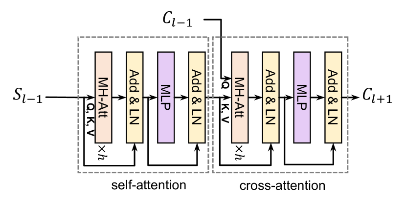
Figure 4: Transformer Encoder Layer.

III-B Progressive Attention Encoder

Existing Transformer-based models [35, 63, 64, 36] are often task-specific and not very flexible to expand according to the task. To enhance the representation of vision and text, two progressive attention encoder (PAE) structures, Spatial-PAE and Temporal-PAE, are designed to perform long-range dependency modeling, which can be used on existing Transformer-based architectures.

III-B1 Transformer Encoder Layer

Transformer Encoder Layer (TEL), as a key component of the Transformer, plays a significant role in natural language processing and computer vision. Our proposed TEL is made up of self-attention [44] and cross-attention [65], as illustrated in Figure 4. Given the packed matrix representations of queries $\bm{Q}\in\mathbb{R}^{d_{k}\times N}$, keys $\bm{K}\in\mathbb{R}^{d_{k}\times N}$, and values $\bm{V}\in\mathbb{R}^{d_{k}\times N}(d_{k}=d/h)$, the scaled dot-product attention is given by

$$\mathrm{MHA}(\bm{Q},\bm{K},\bm{V}) =\left[\mathrm{head}_{1},\mathrm{head}_{2},\ldots,\mathrm{head}_{h}\right]^{\mathrm{T}},$$ (3)

$$\text{where}\ \mathrm{head}_{i} =\mathrm{Softmax}\left(\frac{\bm{Q}^{\mathrm{T}}\bm{W}_{i}^{Q}(\bm{K}^{\mathrm{T}}\bm{W}_{i}^{K})^{\mathrm{T}}}{\sqrt{d}}\right)\bm{V}^{\mathrm{T}}\bm{W}_{i}^{V},$$

where $\bm{W}_{i}^{Q}\in\mathbb{R}^{d_{k}\times d_{k}}$, $\bm{W}_{i}^{K}\in\mathbb{R}^{d_{k}\times d_{k}}$ and $\bm{W}_{i}^{V}\in\mathbb{R}^{d_{k}\times d_{k}}$ are projection matrices, and $\mathrm{Softmax}(\cdot)$ is the softmax function. Different from self-attention, cross-attention merges two sequences regardless of modality. Given two different sequences $\bm{S}_{l-1}\in\mathbb{R}^{d\times N}$ and $\bm{C}_{l-1}\in\mathbb{R}^{d\times N}$, the calculation of TEL (see Figure 4) can be expressed as

$$\bm{S}_{l}=\bm{S}_{l-1}+\mathrm{LN}\left(\mathrm{MHA}\left(\bm{S}_{l-1},\bm{S}_{l-1},\bm{S}_{l-1}\right)\right),$$ (4)

$$\bm{S}_{l+1}=\bm{S}_{l}+\mathrm{LN}\left(\mathrm{MLP}\left(\bm{S}_{l}\right)\right),$$ (5)

$$\bm{C}_{l}=\bm{S}_{l+1}+\mathrm{LN}\left(\mathrm{MHA}\left(\bm{C}_{l-1},\bm{S}_{l+1},\bm{S}_{l+1}\right)\right),$$ (6)

$$\bm{C}_{l+1}=\bm{C}_{l}+\mathrm{LN}\left(\mathrm{MLP}\left(\bm{C}_{l}\right)\right),$$ (7)

where $\mathrm{LN}(\cdot)$ is the layer normlization, $\mathrm{MLP}(\cdot)$ stands for multilayer perceptron, a common feedforward network. For the purpose of description, we define the TEL calculation as $TEL\left(\bm{S}_{l-1},\bm{C}_{l-1}\right)$.

III-B2 Messaging between TELs

Based on the way of message transfer between TELs, we designed two different delivery methods, Spatial-PAE and Temporal-PAE, to enhance the key feature representation, as shown in Figure 5.

Spatial-PAE (see Figure 5(a)) makes a spatial connection to the input sequence of the external source using linear projection. This type of connection is not based on fusion but on cross-attention activation. In long-range dependency modeling with TELs, the self-attention mechanism is limited in capturing global information and requires longer sequence distances to establish connections. Spatial-PAE assists long-range dependency modeling with external knowledge that contains global information to enhance the spatial perception of vision and representation of key features.

Temporal-PAE (see Figure 5(b)) makes a temporal connection to the input sequence of the last moment using linear projection. In TEL, positional encoding may not accurately capture the positional relationships within a sequence. When multiple self-attention layers are stacked, potential ambiguity and inaccuracy in the representation of position information can result in performance degradation. Temporal-PAE calculates the attention map using the sequence output from the previous and current time steps, which helps mitigate the ambiguity and inaccuracy of position information with increasing depth of self-attention layers.

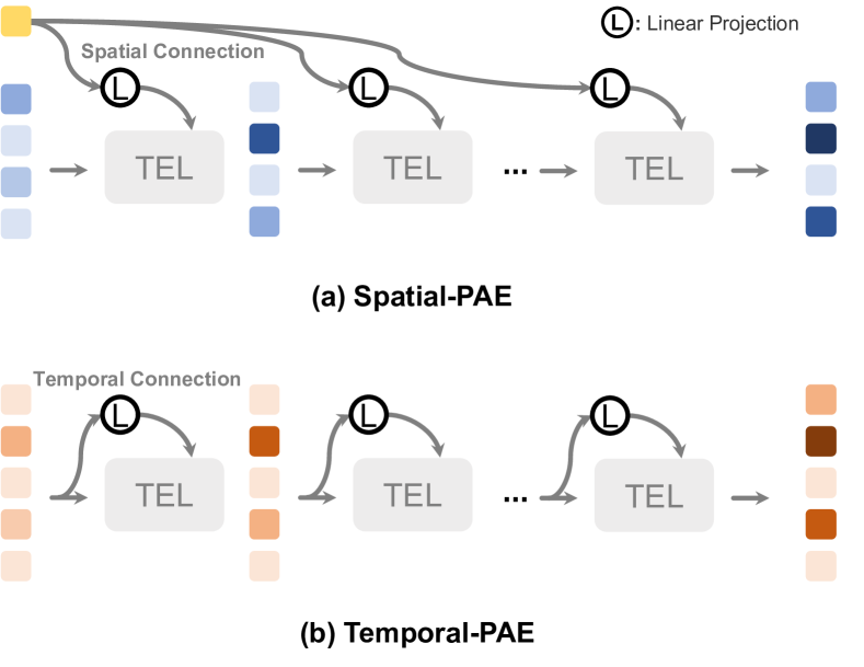
Figure 5: Two different progressive attention encoders (PAE) for messaging: (a) Spatial-PAE and (b) Temporal-PAE.

III-C Vision Instruction Representation

Unlike natural images, small-scale objects in remote sensing images are more likely to be affected by semantic noise, such as background and irrelevant objects, greatly affecting vision representation. Vision Instruction Representation (VIR) firstly construct the belief matrix using instruction embedding and then filter features for an unbiased vision representation, as shown in Figure 2.

The prior knowledge of remote sensing scene recognition $\bm{v}_{ins}$ is used to calculate the belief matrix $\bm{\mathcal{M}}^{\text{bel}}\in\mathbb{R}^{1\times(m+1)}$ on the local correlated features $\left[\bm{v}_{cls},\bm{E}_{v}\right]$, and then sort and filter features with a hard belief strategy as

$$\bm{\mathcal{M}}^{\text{bel}}=\operatorname{Softmax}\left(\bm{v}_{ins}^{\mathrm{T}}\left[\bm{v}_{cls},\bm{E}_{v}\right]\right),$$ (8)

$$\left[\bm{v}_{cls},\bm{E}_{v}\right]\underset{\text{ Sort \& Filter }}{\stackrel{{\scriptstyle\bm{\mathcal{M}}^{\text{bel }}}}{{\longrightarrow}}}\bm{F}_{v}=\left[\bm{f}_{r_{1}},\bm{f}_{r_{2}},\ldots,\bm{f}_{r_{k}}\right],\left(\bm{r}_{k}<m+1\right)$$ (9)

where $\bm{A}\underset{\text{ Sort \& Filter }}{\stackrel{{\scriptstyle\bm{\mathcal{M}}^{\text{bel }}}}{{\longrightarrow}}}\bm{B}$ represents sort and filter the $\bm{A}$ sequence according to $\bm{\mathcal{M}}^{\text{bel}}$ to get the $\bm{B}$ sequence.

To allow dynamic filtering of features, we propose a soft belief strategy without manually setting the number of features $\bm{r}_{k}$. For batch ranking, the rank $\bm{R}_{j}$ of element $\bm{\mathcal{M}}^{\text{bel}}\in\mathbb{R}^{1\times(m+1)}$.

$$\bm{R}_{j}=1+\sum_{k=1}^{m+1}\mathbb{I}\left(\bm{\mathcal{M}}^{\text{bel}}_{k}<\bm{\mathcal{M}}^{\text{bel}}_{j}\right),$$ (10)

where $\mathbb{I}(\cdot)$ is the indicator function to get the ranking weight of belief matrix scores, which is 1 when the condition inside the parenthesis is true, and 0 otherwise. For each element $\bm{F}_{l}$ of dimension $d$ in $\left[\bm{v}_{cls},\bm{E}_{v}\right]\in\mathbb{R}^{d\times(m+1)}$, we get rank-weighted visual features as

$$\bm{F}_{v}=\bm{F}_{l}\left(\bm{\mathcal{M}}^{\text{bel}}_{j}+\frac{1}{\sqrt{\bm{R}_{j}}}\right),$$ (11)

where $\bm{F}_{v}=\left[\bm{f}_{r_{1}},\bm{f}_{r_{2}},\ldots,\bm{f}_{r_{k}}\right],\left(\bm{r}_{k}=m+1\right)$. This strategy is an alternative to Equation 9 does not require setting the feature size. This strategy makes the retrieval faster and better as shown in Table I. We also use this same strategy in PIR-CLIP to learn unbiased visual representation of large-scale data. The VIR of PIR-CLIP can be specified in Algorithm 2.

Then, Spatial-PAE models long-range dependency relationships on the filtered features activated by external information $\bm{V}_{ins}=\left[\bm{v}_{ins},\bm{v}_{ins},\ldots,\bm{v}_{ins}\right]\in\mathbb{R}^{d\times\bm{r}_{k}}$ as

$$\widehat{\bm{F}}^{i}_{v}=\left\{\begin{matrix}\begin{aligned} &TEL\left(\bm{F}_{v},\bm{W}_{s}^{i}\bm{V}_{ins}\right),i=1,\\ &TEL\left(\widehat{\bm{F}}^{i-1}_{v},\bm{W}_{s}^{i}\bm{V}_{ins}\right),i=2,3,\ldots,\bm{n}_{v},\end{aligned}\end{matrix}\right.$$ (12)

where $\widehat{\bm{F}}^{i}_{v}=\left[\widehat{\bm{f}_{r_{1}}^{i}},\widehat{\bm{f}_{r_{2}}^{i}},\ldots,\widehat{\bm{f}_{r_{k}}^{i}}\right]$ is the output of $i$-th TEL, and $\bm{W}_{s}^{i}\in\mathbb{R}^{d\times d}$ denotes the $i$-th weights of linear projection. Then we can get an unbiased local correlated embedding $\bm{v}_{loc}\in\mathbb{R}^{d\times 1}$ as

$$\bm{v}_{loc}=\operatorname{Head}\left(\widehat{\bm{f}_{r_{1}}^{\bm{n}_{v}}}\right),$$ (13)

where $\operatorname{Head}(\cdot)$ represents mapping the head embedding of the last layer to unbiased embedding. To preserve global semantic correlations, the final visual embedding is obtained as $\bm{v}_{emb}=\bm{v}_{cls}+\bm{v}_{loc}$.

III-D Language Cycle Attention

The text encoder based on Transformer has the ability of bidirectional context modeling, but it still has limitations in a modeling context. Transformer is sensitive to sequence location information [44, 66], which does not explicitly process the position information, but introduces position encoding to the input sequence. This may lead to confusion or ambiguity of position information when dealing with long sequences, resulting in reduced sequence representation capability. Language Cycle Attention (LCA) obtains local correlated text features by cyclically activating word-level features from the previous time step to obtain unbiased text representation.

With Temporal-PAE, we can activate text features recursively as

$$\widehat{\bm{F}}^{i}_{t}=\left\{\begin{matrix}\begin{aligned} &TEL\left(\left[\bm{t}_{cls},\bm{E}_{t}\right],\bm{W}_{t}^{i}\left[\bm{t}_{cls},\bm{E}_{t}\right]\right),i=1,\\ &TEL\left(\widehat{\bm{F}}^{i-1}_{t},\bm{W}_{t}^{i}\widehat{\bm{F}}^{i-1}_{t}\right),i=2,3,\ldots,\bm{n}_{t},\end{aligned}\end{matrix}\right.$$ (14)

where $\widehat{\bm{F}}^{i}_{t}=\left[\widehat{\bm{t}_{cls}^{i}},\widehat{\bm{E}_{t}^{i}}\right]$ is the output of $i$-th TEL, $\bm{W}_{t}^{i}\in\mathbb{R}^{d\times d}$ denotes the $i$-th weights of linear projection, and $\widehat{\bm{E}_{t}^{i}}=\left[\widehat{\bm{e}_{1}^{t}},\widehat{\bm{e}_{2}^{t}},\ldots,\widehat{\bm{e}_{n}^{t}}\right]$. Then we can get an unbiased local correlated embedding $\bm{t}_{loc}\in\mathbb{R}^{d\times 1}$ as

$$\bm{t}_{loc}=\operatorname{Head}\left(\widehat{\bm{t}_{cls}^{\bm{n}_{t}}}\right).$$ (15)

Similarly, we add the global correlated feature to get the final text embedding as $\bm{t}_{emb}=\bm{t}_{cls}+\bm{t}_{loc}$.

III-E Loss Function

III-E1 Contrastive Loss

In RSITR, the triplet loss [19] is often used to guide the model optimization. Contrastive loss has a better optimization effect compared to the triplet loss (see Table I comparison of $VSE_{2}$(TL) and $VSE_{2}$(CL), so we use contrastive loss [67] to optimize our model, which only requires computing similarities between two samples without additional negative samples.

Given a mini-batch sample, we follow [27, 68] to randomly sample $N$ positive remote sensing image-text pairs $\left\{(\bm{I}_{1},\bm{T}_{1}),(\bm{I}_{2},\bm{T}_{2}),...,(\bm{I}_{i},\bm{T}_{i}),\dots,(\bm{I}_{N},\bm{T}_{N})\right\}$, with corresponding final vision and text embeddings ($\bm{v}_{emb}$ and $\bm{t}_{emb}$) as $\left\{(\bm{v}_{1},\bm{t}_{1}),(\bm{v}_{2},\bm{t}_{2}),...,(\bm{v}_{i},\bm{t}_{i}),...,(\bm{v}_{N},\bm{t}_{N})\right\}$, and then calculate the cosine similarity as $\bm{s}_{i,j}=\bm{v}_{i}^{\mathrm{T}}\bm{t}_{j}$. So we can get the vision-to-text contrastive loss and text-to-vision contrastive loss as

$$\mathcal{L}_{v2t}\left(\bm{v}_{\bm{i}},\bm{t}_{\bm{i}}\right)=-\log\left(\frac{\exp\left(\bm{s}_{i,i}/\tau\right)}{\sum_{j=1}^{N}\exp\left(\bm{s}_{i,j}/\tau\right)}\right),$$ (16)

$$\mathcal{L}_{t2v}\left(\bm{t}_{\bm{i}},\bm{v}_{\bm{i}}\right)=-\log\left(\frac{\exp\left(\bm{s}_{i,i}/\tau\right)}{\sum_{j=1}^{N}\exp\left(\bm{s}_{j,i}/\tau\right)}\right),$$ (17)

where $\tau$ is the temperature parameter and contrastive loss can be represented as

$$\mathcal{L}_{c}=\frac{1}{2}\sum_{i=1}^{N}\left(\mathcal{L}_{v2t}\left(\bm{v}_{\bm{i}},\bm{t}_{\bm{i}}\right)+\mathcal{L}_{t2v}\left(\bm{t}_{\bm{i}},\bm{v}_{\bm{i}}\right)\right).$$ (18)

III-E2 Affiliation Loss

In current, most retrieval tasks only consider pair-wise losses, such as contrastive loss [27, 68] and triplet loss [19], without a comprehensive consideration of the distribution characteristics of the data, as shown in Figure 6(a). We propose affiliation loss, which minimizes the distance between the modality and the clustering center of the affiliated category based on the distribution characteristics of remote sensing data [24], as shown in Figure 6(b). Affiliation loss is a cluster-wise loss [69] to reduce semantic confusion zones [24], based on the contrastive learning and scene category information.

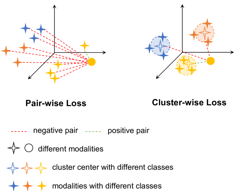
Figure 6: Pair-wise loss and cluster-wise loss.

Figure 7 shows the numpy-like pseudocode of affiliation loss. Given a mini-batch sample, we can categorize them into $C$ classes based on scene category information . For each image, its corresponding text is grouped into one category, so that we can get the positive pairs $\left\{(\bm{v}_{1},\bm{t}_{1}^{*}),(\bm{v}_{2},\bm{t}_{2}^{*}),...,(\bm{v}_{i},\bm{t}_{i}^{*}),\dots,(\bm{v}_{N},\bm{t}_{N}^{*})\right\}$, where $\bm{t}_{i}^{*}$ represents the clustering center corresponding to the $i$-th text. For each text, they are in a similar way as before. We can calculate the cosine similarity of vision-to-text $\bm{s}_{i,j}^{v}=\bm{v}_{i}^{\mathrm{T}}\bm{t}_{j}^{*}$ and the cosine similarity of text-to-vision $\bm{s}_{j,i}^{t}=\bm{t}_{j}^{\mathrm{T}}\bm{v}_{i}^{*}$. Then we can obtain the vision-to-text and text-to-vision attribution loss representations as

$$\mathcal{L}_{v2t}^{*}\left(\bm{v}_{\bm{i}},\bm{t}_{i}^{*}\right)=-\log\left(\frac{\exp\left(\bm{s}_{i,i}^{v}/\tau\right)}{\sum_{j=1}^{N}\exp\left(\bm{s}_{i,j}^{v}/\tau\right)}\right),$$ (19)

$$\mathcal{L}_{t2v}^{*}\left(\bm{t}_{\bm{i}},\bm{v}_{\bm{i}}^{*}\right)=-\log\left(\frac{\exp\left(\bm{s}_{i,i}^{t}/\tau\right)}{\sum_{j=1}^{N}\exp\left(\bm{s}_{j,i}^{t}/\tau\right)}\right),$$ (20)

so affiliation loss can be denoted as

$$\mathcal{L}_{a}=\frac{1}{2}\sum_{i=1}^{N}\left(\mathcal{L}_{v2t}^{*}\left(\bm{v}_{\bm{i}},\bm{t}_{i}^{*}\right)+\mathcal{L}_{t2v}^{*}\left(\bm{t}_{\bm{i}},\bm{v}_{\bm{i}}^{*}\right)\right),$$ (21)

and we can get the final loss function as

$$\mathcal{L}=\mathcal{L}_{c}+\bm{\lambda}_{cs}\mathcal{L}_{a},$$ (22)

where $\bm{\lambda}_{cs}$ is the center scale, indicating the extent of clustering at the category center.

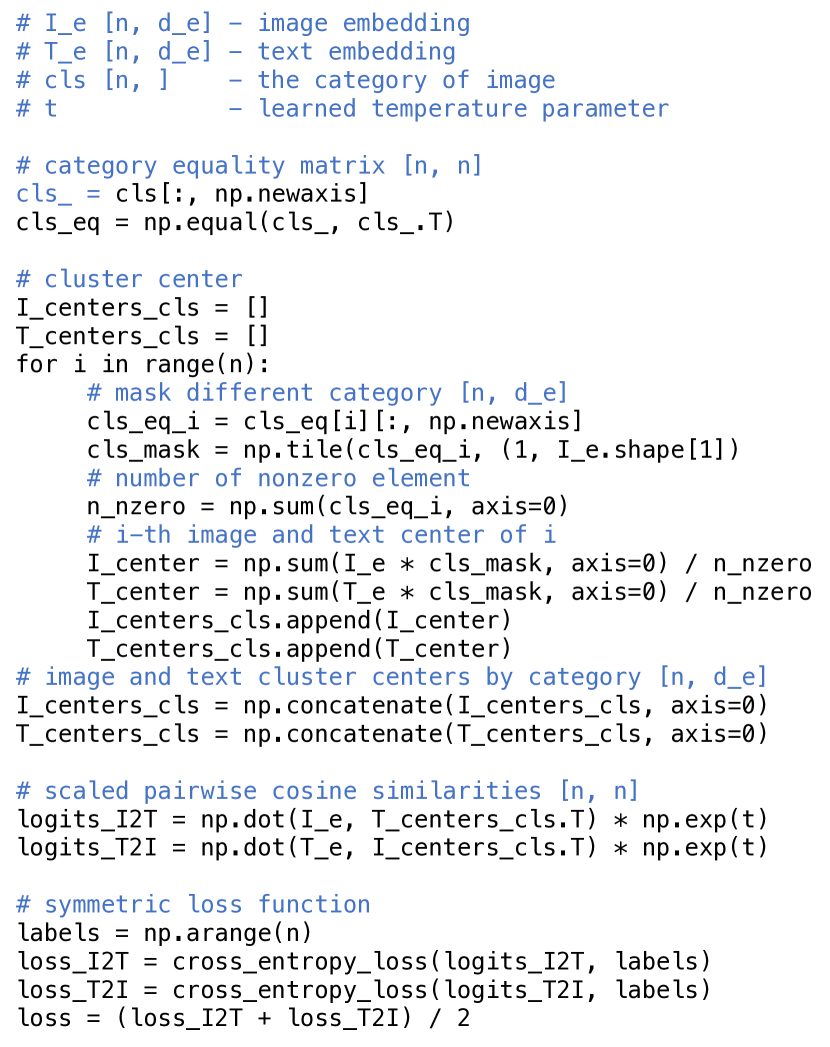
Figure 7: Numpy-like pseudocode of affiliation loss.

III-F Training Paradigm

For PIR-ITR with soft belief strategy, we train on the RSICD dataset [8] or RSITMD dataset [9] as shown in Algorithm 1. We first obtain positive remote sensing image-text pairs $\left\{(\bm{I}_{1},\bm{T}_{1},\bm{S}_{1}),(\bm{I}_{2},\bm{T}_{2},\bm{S}_{2}),\dots,(\bm{I}_{M},\bm{T}_{M},\bm{S}_{M})\right\}$ from the remote sensing image-text datasets $\mathcal{\bm{D}}$. For vision and text encoding, the image $\bm{I}$ and text $\bm{T}$ are encoded separately to obtain the corresponding visual features $\left[\bm{v}_{cls},\bm{E}_{v}\right]$, instruction embeddings $\bm{v}_{ins}$ and textual features $\left[\bm{t}_{cls},\bm{E}_{t}\right]$. For vision instruction representation, we compute the belief matrix $\bm{\mathcal{M}}^{\text{bel}}_{j}$ of visual features and instruction embeddings and calculate the rank $\bm{R}_{j}$ of element $\bm{\mathcal{M}}^{\text{bel}}_{j}$ in batch training. For each element $\bm{F}_{l}$ of dimension $d$ in $\left[\bm{v}_{cls},\bm{E}_{v}\right]\in\mathbb{R}^{d\times(m+1)}$, we get rank-weighted visual features $\bm{F}_{v}$. Then we can use Spatial-PAE and Temporal-PAE to get $\bm{v}_{emb}$ and $\bm{t}_{emb}$ respectively. Notably, the clustering centers for each scene category of each batch need to be computed before calculating affiliation loss. Finally we compute the contrastive loss $\mathcal{L}_{c}$ and affiliation loss $\mathcal{L}_{a}$ to update the model parameters $\emptyset_{s},\emptyset_{b},\emptyset_{sp},\emptyset_{te}$ that require gradient updating.

The PIR-ITR directly performs the PIR learning paradigm after visual and text encoder processing for the above closed-domain retrieval. However, this complex and large structure is not easy to train on large-scale data. For PIR-CLIP, we first pre-train on RS5M dataset [29] using CLIP with contrastive loss, then fine-tune visual representation from RSITR datasets, the fine-tuning procedure of PIR-CLIP as shown in Algorithm 2. The specific fine-tuning process is similar to that of PIR-ITR described above, with the difference that VIR is modified with the base ViT and ResNet models. LCA is replaced with a language Transformer trained on a large-scale remote sensing corpus. Compared to PIR-ITR, PIR-CLIP is a modification of the ViT structure, using convolution to accomplish patching, followed by a soft belief strategy, and then a Transformer encoder to interact between vision features and instruction features. The language encoder trained with the help of large-scale image-text pairs can directly encode the final text embedding without further post-processing by LCA.

Algorithm 1 Training Procedure of PIR-ITR

0:    $M$ positive RS image-text pairs with scene label $\mathcal{\bm{D}}=\left\{(\bm{I}_{1},\bm{T}_{1},\bm{S}_{1}),(\bm{I}_{2},\bm{T}_{2},\bm{S}_{2}),\dots,(\bm{I}_{M},\bm{T}_{M},\bm{S}_{M})\right\}$,

0:    

  for each batch $\bm{I},\bm{T},\bm{S}$ in $\mathcal{\bm{D}}$ do

     Vision and Text Encoding

     Encode visual features $\left[\bm{v}_{cls},\bm{E}_{v}\right]=\mathcal{F}\left(\bm{I};\emptyset_{s}\right)$ and instruction embeddings $\bm{v}_{ins}=\mathcal{R}\left(\bm{I};\emptyset_{r}\right)$;

     Encode text features $\left[\bm{t}_{cls},\bm{E}_{t}\right]=\mathcal{B}\left(\bm{T};\emptyset_{b}\right)$;

     Vision Instruction Representation

     Calculate belief matrix $\bm{\mathcal{M}}^{\text{bel}}_{j}=\operatorname{Softmax}\left(\bm{v}_{ins}^{\mathrm{T}}\left[\bm{v}_{cls},\bm{E}_{v}\right]\right)$;

     Calculate the rank $\bm{R}_{j}$ of element $\bm{\mathcal{M}}^{\text{bel}}_{j}$ in batch;

     for each element $\bm{F}_{l}$ of dimension $d$ in $\left[\bm{v}_{cls},\bm{E}_{v}\right]\in\mathbb{R}^{d\times(m+1)}$ do

        Calculate rank-weighted visual features $\bm{F}_{v}=\bm{F}_{l}\left(\bm{\mathcal{M}}^{\text{bel}}_{j}+\frac{1}{\sqrt{\bm{R}_{j}}}\right)$;

     end for

     Calculate $\bm{v}_{emb}=\textit{Spatial-PAE}\left(\bm{F}_{v},\bm{v}_{ins};\emptyset_{sp}\right)$;

     Language Cycle Attention

     Calculate $\bm{t}_{emb}=\textit{Temporal-PAE}\left(\left[\bm{t}_{cls},\bm{E}_{t}\right];\emptyset_{te}\right)$;

     Loss Function

     Calculate contrastive loss $\mathcal{L}_{c}=\frac{1}{2}\sum_{i=1}^{N}\left(\mathcal{L}_{v2t}\left(\bm{v}_{\bm{i}},\bm{t}_{\bm{i}}\right)+\mathcal{L}_{t2v}\left(\bm{t}_{\bm{i}},\bm{v}_{\bm{i}}\right)\right)$;

     Calculate $C$ classes clustering center based on scene label $\bm{S}$;

     Calculate affiliation loss $\mathcal{L}_{a}=\frac{1}{2}\sum_{i=1}^{N}\left(\mathcal{L}_{v2t}^{*}\left(\bm{v}_{\bm{i}},\bm{t}_{i}^{*}\right)+\mathcal{L}_{t2v}^{*}\left(\bm{t}_{\bm{i}},\bm{v}_{\bm{i}}^{*}\right)\right)$;

     Update $\emptyset_{s},\emptyset_{b},\emptyset_{sp},\emptyset_{te}$;

  end for

  return  $\emptyset_{s},\emptyset_{b},\emptyset_{sp},\emptyset_{te}$

Algorithm 2 Fine-tuning Procedure of PIR-CLIP

0:    $M$ positive RS image-text pairs with scene label $\mathcal{\bm{D}}=\left\{(\bm{I}_{1},\bm{T}_{1},\bm{S}_{1}),(\bm{I}_{2},\bm{T}_{2},\bm{S}_{2}),\dots,(\bm{I}_{M},\bm{T}_{M},\bm{S}_{M})\right\}$,pre-trained instruction encoder weights $\emptyset_{b}$ and instruction encoder weights $\emptyset_{r}$

0:    

  for each batch $\bm{I},\bm{T}$ in $\mathcal{\bm{D}}$ do

     Vision and Text Encoding

     Encode visual features $\left[\bm{v}_{cls},\bm{E}_{v}\right]=\mathcal{F}\left(\bm{I};\emptyset_{c}\right)$ with convolution and instruction embeddings $\bm{v}_{ins}=\mathcal{R}\left(\bm{I};\emptyset_{r}\right)$;

     Encode text features $\left[\bm{t}_{cls},\bm{E}_{t}\right]=\mathcal{B}\left(\bm{T};\emptyset_{b}\right)$;

     Vision Instruction Representation

     Calculate belief matrix $\bm{\mathcal{M}}^{\text{bel}}_{j}=\operatorname{Softmax}\left(\bm{v}_{ins}^{\mathrm{T}}\left[\bm{v}_{cls},\bm{E}_{v}\right]\right)$;

     Calculate the rank $\bm{R}_{j}$ of element $\bm{\mathcal{M}}^{\text{bel}}_{j}$ in batch;

     for each element $\bm{F}_{l}$ of dimension $d$ in $\left[\bm{v}_{cls},\bm{E}_{v}\right]\in\mathbb{R}^{d\times(m+1)}$ do

        Calculate rank-weighted visual features $\bm{F}_{v}=\bm{F}_{l}\left(\bm{\mathcal{M}}^{\text{bel}}_{j}+\frac{1}{\sqrt{\bm{R}_{j}}}\right)$;

     end for

     Calculate $\bm{v}_{emb}=\textit{Transformer}\left(\left[\bm{v}_{ins},\bm{F}_{v}\right];\emptyset_{tr}\right)$;

     Loss Function

     Calculate contrastive loss $\mathcal{L}_{c}=\frac{1}{2}\sum_{i=1}^{N}\left(\mathcal{L}_{v2t}\left(\bm{v}_{\bm{i}},\bm{t}_{\bm{i}}\right)+\mathcal{L}_{t2v}\left(\bm{t}_{\bm{i}},\bm{v}_{\bm{i}}\right)\right)$;

     Calculate $C$ classes clustering center based on scene label $\bm{S}$;

     Calculate affiliation loss $\mathcal{L}_{a}=\frac{1}{2}\sum_{i=1}^{N}\left(\mathcal{L}_{v2t}^{*}\left(\bm{v}_{\bm{i}},\bm{t}_{i}^{*}\right)+\mathcal{L}_{t2v}^{*}\left(\bm{t}_{\bm{i}},\bm{v}_{\bm{i}}^{*}\right)\right)$;

     Update $\emptyset_{c},\emptyset_{tr}$;

  end for

  return  $\emptyset_{c},\emptyset_{tr}$

IV EXPERIMENTS

IV-A Datasets

In our experiments, we use two benchmark datasets RISCD [8] and RSITMD [9], which are commonly used in RSITR [52, 9, 23, 24].

IV-A1 RSICD Dataset

RSICD contains 10,921 images with a resolution of 224 × 224, each with five captions. We follow [9, 23] in dividing 7,862 training images, 1,966 validation images, and 1,093 test images.

IV-A2 RSITMD Dataset

RSITMD contains 4743 images with a resolution of 256 × 256, each with five more fine-grained than RSICD. We follow [23] in 3,435 training images, 856 validation images, and 452 test images.

IV-A3 RS5M Dataset

RS5M [29] contains approximately 5 million remote sensing image-text pairs obtained by filtering publicly available remote sensing image-text datasets and captioning label-only remote sensing datasets with pre-trained image caption models. Our work uses the RS5M dataset as a pre-training dataset for PIR-CLIP.

IV-B Metrics

In accordance with previous RSITR studies [52, 9, 23, 24], we adopt the metrics of $R@K(K=1,5,10)$ and $mR$ to evaluate the effectiveness of our method. $R@K$ measures the percentage of correctly matched pairs within the top $K$ retrieved results, while $mR$ calculates the average of $R@K$ values, providing an overall assessment of the retrieval performance.

IV-C Implementation Details

For closed-domain retrieval, Swin Transformer is used as the vision encoder, pre-trained on ImageNet [70] using Swin-T (tiny version) , and BERT is used as the text encoder with pre-trained parameters from BERT-B (base version) provided by the official source . The output dimensions for both vision and text encodings are set to 768 and then linearly mapped to 512 dimensions. Both self-attention and cross-attention have a head size of 8 and a dropout rate of 0.2, with different numbers of repeat units (2 for Spatial-PAE and 3 for Temporal-PAE). ResNet-50 pre-trained on AID dataset [61] is used as the instruction encoder, with the second-to-last layer as an output of size 1024, linearly mapped to 512 dimensions. The contrastive and attribution losses have a temperature coefficient of 0.07 and a center factor of 1. Training is performed in parallel on 2 NVIDIA RTX A6000 GPUs, with a batch size of 128, using AdamW [71] optimizer with a learning rate of $6e^{-5}$ and weight decay of 0.01. VIR filter size is set to 40 both on RSITMD and RSICD.

For open-domain retrieval, ResNet-50 + ViT-B and Transformer are used as visual and textual backbones to align vanilla CLIP. We train a modified ResNet-50 on the AID dataset [61] and freeze the parameters before the attention pool layer during CLIP tuning. The pre-training epoch is set to 20, the batch size to 256, the fine-tuning is set to 10, and the batch size to 512, and the training samples go through 1,000,000 steps per epoch. The pre-training and fine-tuning of PIR-CLIP is performed on a cluster of 4 NVIDIA A100 GPUs with $1e^{-5}$ learning rate and using automatic mixed-precision. Other settings are the same as for PIR-ITR. Model codes and checkpoints are open-sourced at https://github.com/jaychempan/PIR-CLIP.

TABLE I: Comparison retrieval results of the closed-domain image-text retrieval on RSICD and RSITMD.

			RSICD Dataset			RSITMD Dataset
Method	Params	Backbone vision / text	Image-query-Text R@1 / R@5 / R@10	Text-query-Image R@1 / R@5 / R@10	mR	Image-query-Text R@1 / R@5 / R@10	Text-query-Image R@1 / R@5 / R@10	mR
$VSE_{0}$ [72] (TL)	29 M	ResNet-50 / GRU	4.56 / 16.73 / 22.94	4.37 / 15.37 / 25.35	14.89	9.07 / 21.61 / 31.78	7.73 / 27.80 / 41.00	23.17
SCAN i2t [48]	60 M	RoI Trans / GRU	4.82 / 13.66 / 21.99	3.93 / 15.20 / 25.53	14.19	8.92 / 22.12 / 33.78	7.43 / 25.71 / 39.03	22.83
SCAN t2i [48]	60 M	RoI Trans / GRU	4.79 / 16.19 / 24.86	3.82 / 15.70 / 28.28	15.61	7.01 / 20.58 / 30.90	7.06 / 26.49 / 42.21	22.37
CAMP [52]	63 M	RoI Trans / GRU	4.64 / 14.61 / 24.09	4.25 / 15.82 / 27.82	15.20	8.11 / 23.67 / 34.07	6.24 / 26.37 / 42.37	23.47
CAMERA [73]	64 M	RoI Trans / BERT	4.57 / 13.08 / 21.77	4.00 / 15.93 / 26.97	14.39	8.33 / 21.83 / 33.11	7.52 / 26.19 / 40.72	22.95
LW-MCR [52]	-	CNNs / CNNs	3.29 / 12.52 / 19.93	4.66 / 17.51 / 30.02	14.66	10.18 / 28.98 / 39.82	7.79 / 30.18 / 49.78	27.79
AMFMN [9]	36 M	ResNet-18 / GRU	5.21 / 14.72 / 21.57	4.08 / 17.00 / 30.60	15.53	10.63 / 24.78 / 41.81	11.51 / 34.69 / 54.87	29.72
GaLR [23]	46 M	ResNet-18+ppyolo / GRU	6.59 / 19.85 / 31.04	4.69 / 19.48 / 32.13	18.96	14.82 / 31.64 / 42.48	11.15 / 36.68 / 51.68	31.41
KCR [22]	-	ResNet-101 / BERT	5.95 / 18.59 / 29.58	5.40 / 22.44 / 37.36	19.89	-	-	-
SWAN [24]	40 M	ResNet-50 / GRU	7.41 / 20.13 / 30.86	5.56 / 22.26 / 37.41	20.61	13.35 / 32.15 / 46.90	11.24 / 40.40 / 60.60	34.11
HVSA [74]	-	ResNet-50 / GRU	7.47 / 20.62 / 32.11	5.51 / 21.13 / 34.13	20.61	13.20 / 32.08 / 45.58	11.43 / 39.20 / 57.45	33.16
DOVE [75]	38 M	ResNet-50+RoI Trans / GRU	8.66 / 22.35 / 34.95	6.04 / 23.95 / 40.35	22.72	16.81 / 36.80 / 49.93	12.20 / 49.93 / 66.50	37.73
$VSE_{1}$ (CL)	131 M	ViT-B / BERT	9.06 / 22.78 / 32.75	5.32 / 19.47 / 33.71	20.52	12.83 / 31.19 / 46.24	9.60 / 36.59 / 54.42	31.81
$VSE_{2}$ (TL)	137 M	Swin-T / BERT	7.96 / 21.68 / 34.31	6.44 / 22.09 / 37.49	21.66	17.70 / 36.28 / 48.67	13.58 / 41.24 / 59.29	36.13
$VSE_{2}$ (CL)	137 M	Swin-T / BERT	10.52 / 25.07 / 36.78	6.11 / 23.64 / 38.28	23.40	16.15 / 40.04 / 53.10	10.75 / 38.98 / 60.18	36.53
$VSE_{2}$+$TEL$	161 M	Swin-T / BERT	10.43 / 25.89 / 37.15	6.02 / 23.42 / 38.30	23.53	17.48 / 36.95 / 50.44	11.81 / 41.99 / 61.77	36.74
PIR-ITR with hard	161 M	Swin-T+ResNet-50 / BERT	9.88 / 27.26 / 39.16	6.97 / 24.56 / 38.92	24.46	18.14 / 41.15 / 52.88	12.17 / 41.68 / 63.41	38.24
PIR-ITR with soft	161 M	Swin-T+ResNet-50 / BERT	10.89 / 26.17 / 37.79	7.17 / 25.07 / 41.06	24.69	18.36 / 42.04 / 55.53	13.36 / 44.47 / 61.73	39.25

TABLE II: Comparison retrieval results of the open-domain image-text retrieval on RSICD and RSITMD. $\dagger$ is zero-shot CLIP and $\ddagger$ is fine-tune CLIP.

RSICD Dataset
Method	Prams	Backbone vision / text	Pre-training Dataset	Fine-tuning Dataset	Image-query-Text R@1 / R@5 / R@10	Text-query-Image R@1 / R@5 / R@10	mR
CLIP $\dagger$ [27]	151 M	ViT-B / Transformer	WIT (CLIP)	-	4.76 / 12.81 / 19.12	4.70 / 15.43 / 25.01	13.64
CLIP-FT $\ddagger$ [27]	151 M	ViT-B / Transformer	WIT (CLIP)	RSICD	15.55 / 30.56 / 41.99	14.68 / 33.63 / 42.71	29.85
PE-RSITR $\ddagger$ [76]	151 M	ViT-B / Transformer	WIT (CLIP)	RSICD	14.13 / 31.51 / 44.78	11.63 / 33.92 / 50.73	31.12
RemoteCLIP $\dagger$ [28]	151 M	ViT-B / Transformer	RET-3 + DET-10 + SEG-4	-	17.02 / 37.97 / 51.51	13.71 / 37.11 / 54.25	35.26
RemoteCLIP $\dagger$ [28]	428 M	ViT-L / Transformer	RET-3 + DET-10 + SEG-4	-	18.39 / 37.42 / 51.05	14.73 / 39.93 / 56.58	36.35
SkyCLIP $\dagger$ [30]	151 M	ViT-B / Transformer	Skyscript	-	6.59 / 16.10 / 26.53	7.14 / 22.34 / 34.29	18.83
SkyCLIP $\dagger$ [30]	428 M	ViT-L / Transformer	Skyscript	-	7.04 / 17.75 / 27.08	6.40 / 21.21 / 34.00	18.91
GeoRSCLIP $\dagger$ [29]	151 M	ViT-B / Transformer	RS5M	-	11.53 / 28.55 / 39.16	9.52 / 27.37 / 40.99	26.18
GeoRSCLIP-FT $\ddagger$ [29]	151 M	ViT-B / Transformer	RS5M	RSICD	22.14 / 40.53 / 51.78	15.26 / 40.46 / 57.79	38.00
GeoRSCLIP-FT $\ddagger$ [29]	151 M	ViT-B / Transformer	RS5M	RET-2	21.13 / 41.72 / 55.63	15.59 / 41.19 / 57.99	38.87
PIR-CLIP $\ddagger$	189 M	ResNet-50+ViT-B / Transformer	RS5M	RSICD	26.62 / 40.71 / 50.32	21.35 / 43.59 / 54.27	39.48
PIR-CLIP $\ddagger$	189 M	ResNet-50+ViT-B / Transformer	RS5M	RET-2	25.62 / 43.18 / 53.06	19.91 / 42.74 / 55.15	39.95
PIR-CLIP $\ddagger$	189 M	ResNet-50+ViT-B / Transformer	RS5M	RET-3	27.63 / 45.38 / 55.26	21.10 / 44.87 / 56.12	41.73
RSITMD Dataset
CLIP $\dagger$ [27]	151 M	ViT-B / Transformer	WIT (CLIP)	-	5.31 / 17.26 / 25.00	5.84 / 22.74 / 34.82	18.50
CLIP-FT $\ddagger$ [27]	151 M	ViT-B / Transformer	WIT (CLIP)	RSITMD	25.00 / 48.23 / 62.17	23.72 / 49.38 / 63.63	45.35
PE-RSITR $\ddagger$ [76]	151 M	ViT-B / Transformer	WIT (CLIP)	RSITMD	23.67 / 44.07 / 60.36	20.10 / 50.63 / 67.97	44.47
RemoteCLIP $\dagger$ [28]	151 M	ViT-B / Transformer	RET-3 + DET-10 + SEG-4	-	27.88 / 50.66 / 65.71	22.17 / 56.46 / 73.41	49.38
RemoteCLIP $\dagger$ [28]	428 M	ViT-L / Transformer	RET-3 + DET-10 + SEG-4	-	28.76 / 52.43 / 63.94	23.76 / 59.51 / 74.73	50.52
SkyCLIP $\dagger$ [30]	151 M	ViT-B / Transformer	Skyscript	-	10.18 / 25.44 / 35.62	10.88 / 33.27 / 49.82	27.54
SkyCLIP $\dagger$ [30]	428 M	ViT-L / Transformer	Skyscript	-	12.61 / 28.76 / 38.05	10.62 / 34.73 / 51.42	29.37
GeoRSCLIP $\dagger$ [29]	151 M	ViT-B / Transformer	RS5M	-	19.03 / 34.51 / 46.46	14.16 / 42.39 / 57.52	35.68
GeoRSCLIP-FT $\ddagger$ [29]	151 M	ViT-B / Transformer	RS5M	RSITMD	30.09 / 51.55 / 63.27	23.54 / 57.52 / 74.60	50.10
GeoRSCLIP-FT $\ddagger$ [29]	151 M	ViT-B / Transformer	RS5M	RET-2	32.30 / 53.32 / 67.92	25.04 / 57.88 / 74.38	51.81
PIR-CLIP $\ddagger$	189 M	ResNet-50+ViT-B / Transformer	RS5M	RSITMD	30.97 / 58.19 / 71.02	25.62 / 55.27 / 75.00	52.68
PIR-CLIP $\ddagger$	189 M	ResNet-50+ViT-B / Transformer	RS5M	RET-2	44.25 / 65.71 / 75.22	28.45 / 54.65 / 68.05	56.05
PIR-CLIP $\ddagger$	189 M	ResNet-50+ViT-B / Transformer	RS5M	RET-3	45.58 / 65.49 / 75.00	30.13 / 55.44 / 68.54	56.70

IV-D Performance Comparisons

In this section, we compare the proposed PIR-ITR with the state-of-the-art methods on RSICD and RSITMD. Image-query-Text (I2T) and Text-query-Image (T2I) retrieval results are counted for the experiments. Experiments are repeated three times to ensure reliability, and then the average results are taken as the final results.

IV-D1 State-of-the-art methods

We compare and analyze the closed-domain and open-domain methods separately.

Closed-domain methods can be divided into three groups: traditional image-text retrieval methods, $VSE_{0}$ [72], SCAN [48], CAMP [52], and CAMERA [73], remote sensing image-text retrieval methods, LW-MCR [52], AMFMN [9], GaLR [23], KCR [22], SWAN [24], HVSA [74], and DOVE [75], and Transformer-based backbone methods, $VSE_{1}$, $VSE_{2}$ [72] and $VSE_{2}+TEL$.

Most of the above methods are based on different vision and text feature extraction backbones. We use the provided source code for implementation for traditional image-text retrieval methods. For SCAN, CAMP, and CAMERA, RoI Trans [77] with ResNet-50 as backbone pre-trained on DOTA [78] is used to detect significant objects. For remote sensing image-text retrieval methods, we pick the best results from the original paper to make the experiments as fair as possible since the experiments are difficult to be reproduced on RSICD and RSITMD. To be as fair as possible, we add Transformer-based backbone methods compared with PIR-ITR, a further improvement of the $VSE$ method. $VSE_{i}(i=0,1,2)$ represents different vision and text backbones and TEL denotes the Transformer encoder layer. We also marked the corresponding loss function on the method (TL: triplet loss, CL: contrastive loss). “PIR-ITR with hard” and “PIR-ITR with soft” is PIR-ITR with hard and soft belief strategy.

Open-domain methods is to train a visual-semantic embedding model (VSE) with a dual-tower structure using natural language-supervised visual representations on large-scale image-text pairs dataset. CLIP [27], RemoteCLIP [28], GeoRSCLIP [29] and SkyCLIP [30] are respectively trained on WIT, RET-3 + DET-10 + SEG-4, RS5M and SkyScript, as shown in Table II. RET-3 is a combination of RSICD, RSITMD and UCM-Captions [79] datasets and follows the same method of de-duplication as RmoteCLIP [28] to avoid data leakage. We add RET-2 followed by GeoRSCLIP [29], a combination of RSICD and RSITMD that is also de-duplicated. We denote the official CLIP of 400 million image-text pairs from the Internet as WIT(CLIP). According to data availability, we pre-train our proposed PIR-CLIP on the RS5M dataset [29], which is the largest remote sensing image-text pairs dataset to our knowledge. Except for CLIP and SkyCLIP, which are chosen to be obtained by testing based on official weights, the results of the other methods are obtained from the original papers.

IV-D2 Quantitative comparison of Closed-domain methods

The experiments of closed-domain methods focus on the comparison of retrieval performance in a single dataset training and testing, as shown in Table I.

Quantitative comparison on RSICD. As shown in Table I, the remote sensing image-text retrieval method could perform better than the traditional image-text retrieval method. For Transformer-based backbone methods, we can find that using Swin Transformer [63] to extract vision features is superior to ViT [35]. Comparing $VSE_{2}$ (TL) and $VSE_{2}$ (CL), it is found that the method using contrastive loss is better than the method using triplet loss. It is observed that the retrieval performance differs significantly with different vision and text backbones, where Swin-T+BERT $>$ ViT+BERT $>$ ResNet-50+GRU. We can find that Transformer has a better representation in RSITR than CNN. We can find that $mR$ can reach 23.53 when using a combination of $VSE_{2}$+$TEL$, but the improvement is insignificant compared to $VSE_{2}$. Our proposed method can significantly improve the overall retrieval performance, with $mR$ reaching 24.69, an improvement of 4.9% (24.69 vs 23.53).

Quantitative comparison on RSITMD. Compared with RSICD, RSITMD has a more fine-grained text description. Therefore, the retrieval performance of RSITMD is significantly higher than RSICD’s. As shown in Table I, traditional image-text retrieval methods perform unsatisfactorily on RSITMD and RSICD. For the remote sensing image-text retrieval methods, SWAN based on the CNN and GRU feature extraction method makes $mR$ reach 34.11. For Transformer-based feature extraction methods, $VSE_{2}+TEL$ makes $mR$ reach 36.74. Our proposed method results in a 4.0% improvement in $mR$ (39.24 vs 37.73), with I2T $R@1$ and T2I $R@1$ reaching 18.36 and 13.36, respectively.

IV-D3 Quantitative comparison of Open-domain methods

The experiments of open-domain methods is fine-tuned on a small dataset after pre-training on an additional large-scale dataset, as shown in Table II.

Quantitative comparison on RSICD. A comparison of the zero-shot CLIP results reveals that the retrieval performance of pre-training on different large-scale datasets varies significantly, with RemoteCLIP reaching 36.35 on the RSICD dataset. From the results of the RemoteCLIP and SkyCLIP experiments, we found that their ViT-L version of CLIP can only get a limited improvement compared to the ViT-B version. The pre-trained CLIP model on the massive WIT (CLIP) dataset can improve the $mR$ from 13.64 to 29.85 after fine-tuning the RSICD dataset. Further fine-tuning on the RSITR dataset can further improve the performance of the retrieval dataset; GeoRSCLIP, fine-tuned on RET-2, can get $mR$ results 38.87. PIR-CLIP fine-tuned on RSICD, RET-2, and RET-3 allowed further $mR$ enhancement of 1.5%, 2.7%, and 7.3%, respectively, compared to the state-of-the-art method (38.87). Among them, our method has the largest $R@1$ enhancement for I2T and T2I, reaching 27.63 and 21.35. The above experimental results show that our two-stage CLIP-based PIR-CLIP method is important in enhancing the performance of image retrieval and text retrieval $R@1$.

Quantitative comparison on RSITMD. On the RSITMD dataset, RemoteCLIP achieved 50.52 on $mR$ by relying on zero-shot capability. The pre-trained CLIP model on the massive WIT (CLIP) dataset can improve the $mR$ from 18.50 to 45.35 after fine-tuning the RSITMD dataset. Compared to RemoteCLIP (ViT-L), which incorporates RET-3 in its pre-training stage, our PIR-CLIP improves $mR$ by 9.6% with smaller parameters. GeoRSCLIP allows $mR$ to reach 51.81 by fine-tuning on RET-2. PIR-CLIP fine-tuned on RSITMD, RET-2, and RET-3 allowed further $mR$ enhancement of 1.7%, 8.2%, and 9.4%, respectively, compared to the state-of-the-art method (51.81). Among them, our method has the largest $R@1$ enhancement for I2T and T2I, reaching 45.58 and 30.13. The above results show that our proposed PIR-CLIP can enhance visual representation and improve retrieval performance using the vision instruction fine-tuning approach.

IV-D4 Visualization of results

Figure 8 visualizes the top 5 retrieval results, including Image-query-Text (left) and Text-query-Image (right). In Image-query-Text, the blue box represents the query, the green text represents the mutual matching retrieval results, and the red one indicates the mismatched results; in Text-query-Image, the blue text represents the query, the green box represents the mutual matching retrieval results, and the red one indicates the mismatched results. In Image-query-Text, most of the top 5 retrieval results are matching text for an image with only five matching texts. In Text-query-Image, matching images among the top 5 retrieval results rank first or second for a text with only one matching image. We find that PIR-CLIP will outperform PIR-ITR in image and text retrieval. However, in Text-query-Image results, the top 5 returned image retrieval results of PIR-ITR are more similar, and the retrieval results of PIR-CLIP have a higher rank, with the differences in the top 5 returned results being more significant. However, some retrieval results are also similar in semantics to distinguished, indicating that there is still room for further improvement.

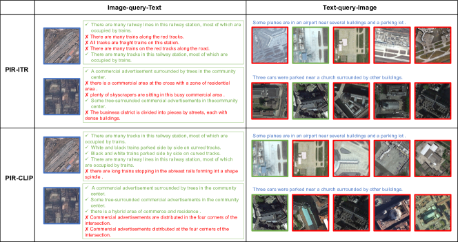
Figure 8: The visualization of the top 5 retrieval results includes Image-query-Text (left) and Text-query-Image (right). Blue text and boxes represent queries, green text and boxes represent matching retrieval results, and red text and boxes indicate mismatched retrieval results.

IV-E Ablation Studies

In this section, we design twelve sets of experiments (the first eight is for PIR-ITR, else for PIR-CLIP) to demonstrate the effectiveness of the proposed three modules VIR, LCR and affiliation loss ($\mathcal{L}_{a}$), as shown in Table III. The baseline group represents the removal of the above three modules as the blank control group. CLIP-baseline is PIR-CLIP removes VIR and attribution loss; other conditions remain the same.

IV-E1 Effects of Vision Instruction Representation

From the experimental results of +VIR, we find that using VIR alone leads to a small increase in $mR$ compared to the experimental results of baseline, with a significant increase in T2I $R@1$. From the experimental results of +VIR+LCA, we find that VIR increases $mR$ from 36.95 to 37.25 compared to the experimental results of +LCA, where VIR increases more for I2T $R@10$ and T2I $R@10$. From the experimental results of +VIR+LCA+$\mathcal{L}_{a}$, $mR$ is improved by 2.6% compared to the experimental results of +LCA+$\mathcal{L}_{a}$, where I2T $R@1$ increases from $17.04$ to $18.14$ and T2I $R@1$ increases from $11.81$ to $12.17$. For PIR-CLIP, we find that VIR increases $mR$ from 45.35 to 48.02 compared with the experimental results of +VIR $\dagger$ and CLIP-baseline, and increases $mR$ from 48.16 to 52.68 compared with the experimental results of +$\mathcal{L}_{a}$ and +VIR $\dagger$ +$\mathcal{L}_{a}$. With the above results, we find that VIR can significantly improve vision representation and enhance the ability of Text-query-Image.

TABLE III: Results of ablation experiments with different modules on the RSITMD test set. Unlike the VIR of PIR-ITR, this VIR $\dagger$ of PIR-CLIP is based on a modified ViT.

Method	Image-query-Text R@1 / R@5 / R@10	Text-query-Image R@1 / R@5 / R@10	mR
baseline	16.15 / 40.04 / 53.10	10.75 / 38.98 / 60.18	36.53
+VIR	16.59 / 38.50 / 54.65	12.88 / 40.04 / 58.19	36.81
+LCA	20.13 / 41.15 / 53.10	14.60 / 38.89 / 53.81	36.95
+$\mathcal{L}_{a}$	19.25 / 36.95 / 52.88	10.88 / 39.51 / 59.87	36.56
+VIR+LCA	17.04 / 39.16 / 54.42	13.50 / 40.04 / 59.34	37.25
+VIR+$\mathcal{L}_{a}$	16.81 / 40.04 / 55.31	11.59 / 41.50 / 61.02	37.71
+LCA+$\mathcal{L}_{a}$	17.04 / 38.72 / 53.76	11.81 / 41.64 / 60.58	37.26
+VIR+LCA+$\mathcal{L}_{a}$	18.14 / 41.15 / 52.88	12.17 / 41.68 / 63.41	38.24
CLIP-baseline	25.00 / 48.23 / 62.17	23.72 / 49.38 / 63.63	45.35
+VIR $\dagger$	24.56 / 53.32 / 66.37	21.02 / 51.86 / 71.02	48.02
+$\mathcal{L}_{a}$	27.65 / 52.21 / 63.94	25.49 / 53.10 / 66.59	48.16
+VIR $\dagger$ +$\mathcal{L}_{a}$	30.97 / 58.19 / 71.02	25.62 / 55.27 / 75.00	52.68

TABLE IV: Results of experiments of filter size in VIR on the RSITMD test set.

VIR Filter Size	Image-query-Text R@1 / R@5 / R@10	Text-query-Image R@1 / R@5 / R@10	mR
$\bm{r}_{k}$=10 with hard	17.26 / 40.71 / 54.65	13.01 / 41.06 / 61.19	37.98
$\bm{r}_{k}$=20 with hard	17.48 / 39.60 / 52.21	13.50 / 42.48 / 62.74	38.00
$\bm{r}_{k}$=30 with hard	19.03 / 37.83 / 49.78	12.83 / 41.90 / 62.08	37.24
$\bm{r}_{k}$=40 with hard	18.14 / 41.15 / 52.88	12.17 / 41.68 / 63.41	38.24
$\bm{r}_{k}$=50 with hard	18.36 / 37.61 / 50.88	13.10 / 42.88 / 62.04	37.48
$\bm{r}_{k}$=50 with soft	18.36 / 42.04 / 55.53	13.36 / 44.47 / 61.73	39.25

IV-E2 Effects of Language Cycle Attention

From the experimental results of +LCA, we find that LCA can respectively improve 24.6% and 35.8% on I2T $R@1$ and T2I $R@1$ compared to the experimental results of baseline. From the experimental results of +VIR+LCA, we can observe that a 1.2% improvement in $mR$ compared to the experimental results of +VIR. From the experimental results of +VIR+LCA+$\mathcal{L}_{a}$, LCA results in a 1.4% improvement in $mR$ compared to the experimental results of +VIR+$\mathcal{L}_{a}$, where I2T $R@1$ is improved from 16.81 to 18.14 and T2I $R@1$ is improved from 11.59 to 12.17. Comparing the experimental group +VIR with +VIR+LCA and the experimental group +$\mathcal{L}_{a}$ with +LCA+$\mathcal{L}_{a}$, we find that the effect of LCA on the Image-query-Text and Text-query-Image task is positive. With the above results, we find that LCA balances with vision representation to improve retrieval performance.

IV-E3 Effects of Affiliation Loss

From the experimental results of +$\mathcal{L}_{a}$, we find that $\mathcal{L}_{a}$ alone can significantly improve I2T $R@1$ compared to the experimental results of baseline, which is improved from 16.15 to 19.25. From the experimental results of +VIR+LCA+$\mathcal{L}_{a}$, it can be observed affiliation loss could improve $mR$ by 2.7% compared to the experimental results of +VIR+LCA, where I2T $R@1$ is improved from 17.04 to 18.14. For PIR-CLIP, we find that $\mathcal{L}_{a}$ increases $mR$ from 45.35 to 48.16 compared with the experimental results of +$\mathcal{L}_{a}$ and CLIP-baseline, and increases $mR$ from 48.02 to 52.68 compared with the experimental results of +VIR $\dagger$ and +VIR $\dagger$ +$\mathcal{L}_{a}$. From the above results, we can conclude that affiliation loss can significantly improve vision and text representations, which can help VIR and LCA to perform long-range dependency modeling.

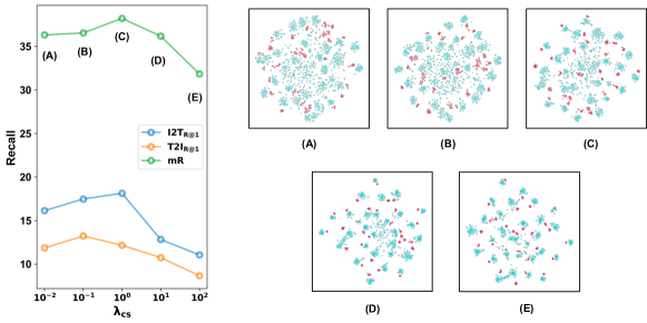
Figure 9: The effect of the center scale on retrieval results (left) and RSITMD test set visualized with t-SNE [33] in the embedding space (right), the red squares represent vision embeddings, and the blue triangles represent text embeddings.

IV-F Parameter Evaluation

There are two important parameters in our proposed modules: the filter size in VIR and the center scale of affiliation loss. This section focuses on experiments to select the appropriate parameters and verify further the roles played in the retrieval process.

IV-F1 Filter Size in VIR

For PIR-ITR with hard belief strategy, the visual features extracted based on Transformer contain much semantic noise, and some of the key features are more representative of the visual representation, so we use VIR for unbiased correction of the visual representation. The maximum number of Vision Transformer output features is 50, and we control the number of key features by adjusting the filter size. Table IV shows the bidirectional retrieval results on the RSITMD with different filter sizes $\bm{r}_{k}$ (see Equation 9). We can find that when $\bm{r}_{k}$=10, I2T $R@10$ is the largest, reaching 54.65; when $\bm{r}_{k}$=20, $mR$ reaches 38.00, and T2I $R@1$ is the largest, reaching 13.50; when $\bm{r}_{k}$=30, I2T $R@10$ is the largest, but $mR$ are relatively low compared to others; when $\bm{r}_{k}$=40, $mR$ is the largest, reaching 38.24, and the key feature is more representative of visual features at this time; when $\bm{r}_{k}$=50, $mR$ is 37.48 smaller than $\bm{r}_{k}$=10, 20, 40 indicating that some key features are susceptible to deactivation by semantic noise. For PIR-ITR with soft belief strategy, it can further enhance the image retrieval and text retrieval performance with $mR$ reaching up to 39.25. From the above experimental results, it can be concluded that semantic noise contained in remote-sensing images deactivates key features, and the retrieval performance can be effectively improved by reducing the dependence on partial features.

IV-F2 Center Scale of Affiliation Loss

The affiliation loss is used to reduce the semantic confusion region in the common subspace, and choosing an appropriate loss factor can improve the bidirectional retrieval performance. Since affiliation loss affects the degree of aggregation within a class, we also refer to this loss factor as the center scale, which measures the degree of aggregation within a class. The left side of Figure 9 shows the retrieval performance on the RSITMD at different center scales $\bm{\lambda}_{cs}$, and the right side corresponds to the visualization of the embedding space at different center scales. As the center scale increases, the inter-class constraints are enhanced, and the semantic confusion zones are gradually reduced (A to E of Figure 9). However, the retrieval performance shows an increase followed by a decrease, indicating that a proper center scale ($\bm{\lambda}_{cs}=10^{0}$) can effectively improve the retrieval performance, and too strong inter-class constraints do not necessarily improve the retrieval performance.

IV-G Instruction Strategy Analysis

To explore the impact of different instruction strategies on retrieval performance, we use different types of models as instruction encoders on PIR-ITR with hard belief strategy, where each model is pre-trained on the AID [61], RESISC45 dataset [80] and ImageNet [81] datasets for the classification task. These are divided into two categories, the CNN-based encoders, including VGG16 [82], VGG-19 [82], ResNet-50 [60], and ResNet-101 [60], and the Transformer-based encoders, including ViT [35] and Swin-T [63]. Table V shows the experimental results of the instruction encoders on the RSITMD dataset. The experimental results show that using ResNet-50 pre-trained on the AID dataset and RESISC45 dataset as the instruction encoder is more effective, performing the best at 38.24 and 38.28. We find no significant increase on retrieval performance by looking at the pre-trained ViT and Swin-T on the AID dataset as instruction encoders. By comparing VGG-16 and ResNet-50 pre-trained on ImageNet, we find that the pre-training based on remote sensing scene classification has a more obvious instructive role in guiding the vision representation. The above experimental results show that using prior knowledge based on remote sensing scene recognition can enhance vision representation and, thus, retrieval performance.

TABLE V: Results of experiments of different instruction strategy on the RSITMD test set.

Instruction Encoder	Pre-trained Dataset	Image-query-Text R@1 / R@5 / R@10	Text-query-Image R@1 / R@5 / R@10	mR
VGG-16	AID	16.15 / 37.61 / 52.21	11.77 / 40.88 / 61.95	36.76
VGG-19	AID	19.47 / 38.94 / 53.10	12.52 / 39.91 / 61.28	37.54
ResNet-50	AID	18.14 / 41.15 / 52.88	12.17 / 41.68 / 63.41	38.24
ResNet-101	AID	17.26 / 39.38 / 52.88	11.81 / 41.02 / 61.55	37.32
ViT	AID	15.71 / 37.39 / 51.11	12.43 / 41.73 / 60.18	36.42
Swin-T	AID	15.93 / 36.28 / 53.32	12.65 / 41.68 / 60.84	36.78
VGG-16	ImageNet	16.81 / 36.28 / 49.12	12.70 / 41.28 / 62.04	36.37
ResNet-50	ImageNet	16.81 / 38.27 / 52.21	13.81 / 41.68 / 61.64	37.40
Swin-T	ImageNet	15.71 / 40.93 / 52.65	13.01 / 40.31 / 60.18	37.13
VGG-16	RESISC45	16.81 / 38.27 / 50.66	11.50 / 40.58 / 60.31	36.36
ResNet-50	RESISC45	17.70 / 39.82 / 53.98	12.92 / 42.96 / 62.30	38.28
Swin-T	RESISC45	15.93 / 37.61 / 52.21	12.08 / 41.06 / 61.37	36.71

V CONCLUSION

This paper proposes the PIR framework, a new paradigm that leverages prior knowledge from the remote sensing data domain for adaptive learning of vision and text representations. We first propose the PIR-ITR for remote sensing image-text retrieval. Notably, Spatial-PAE and Temporal-PAE are applied to perform long-range dependency modelling to enhance key feature representation. In vision representation, VIR based on Spatial-PAE utilizes prior knowledge from remote sensing scene recognition to instruct unbiased vision representation and reduce semantic noise’s impact. In text representation, LCA based on Temporal-PAE activates the current time step based on the previous time step to enhance semantic representation capability. Finally, a cluster-wise attribution loss is used as an inter-class constraint to reduce semantic confusion zones in the common subspace. Building on this foundation, we propose PIR-CLIP to address semantic noise in remote sensing vision-language representations and enhance open-domain retrieval performance further. Comprehensive experiments are designed to validate the superiority and effectiveness of our approach on two benchmark datasets, RSICD and RSITMD.

In the future, a unified multimodal remote sensing foundation model that is more specific to understanding complex multimodal data from remote sensing should be proposed.

Jiancheng Pan (Student Member, IEEE) received the B.E. degree from Jiangxi Normal University, Nanchang, China, in 2022. He is currently pursuing the M.E. degree with the Zhejiang University of Technology, Hangzhou, China. His research interests include but are not limited to Cross-modal Retrieval, Vision-Language Models, and AI for Science.

Muyuan Ma received the B.E. Degree from the School of Marine Science and Technology, Tianjin University, Tianjin, China, in 2022. He is currently pursuing the PhD degree in the Department of Earth System Science, Tsinghua University, Beijing, China. His research interests include Computer Vision, deep learning applications in remote sensing and AI for Science.

Qing Ma received the B.S. and M.S. degrees from Beijing Normal University, Beijing, China, in 2002 and 2005, respectively, and the Ph.D. degree from the Zhejiang University of Technology, Hangzhou, China, in 2021. Since 2005, she has been on the faculty of the College of Science, Zhejiang University of Technology. Her research interests include cross-modal retrieval and computer vision.

Cong Bai (Member, IEEE) received the B.E. degree from Shandong University, Jinan, China, in 2003, the M.E. degree from Shanghai University, Shanghai, China, in 2009, and the Ph.D. degree from the National Institute of Applied Sciences, Rennes, France, in 2013. He is a Professor with the College of Computer Science and Technology, Zhejiang University of Technology, Hangzhou, China. His research interests include computer vision and multimedia processing.

Shengyong Chen (Senior Member, IEEE) received the Ph.D. degree in computer vision from the City University of Hong Kong, Hong Kong, in 2003. He was with the University of Hamburg, Hamburg, Germany, from 2006 to 2007. He is currently a Professor with the Tianjin University of Technology, Tianjin, China, and with the Zhejiang University of Technology, Hangzhou, China. He has authored over 100 scientific articles in international journals. His research interests include computer vision, robotics, and image analysis. Dr. Chen is a fellow of the IET and a Senior Member of the CCF. He received the National Outstanding Youth Foundation Award of China in 2013. He also received the fellowship from the Alexander von Humboldt Foundation of Germany.

References

- [1] H. Guo, X. Su, C. Wu, B. Du, and L. Zhang, “Saan: Similarity-aware attention flow network for change detection with vhr remote sensing images,” IEEE Transactions on Image Processing, vol. 33, pp. 2599–2613, 2024.
- [2] Q. He, X. Sun, W. Diao, Z. Yan, F. Yao, and K. Fu, “Multimodal remote sensing image segmentation with intuition-inspired hypergraph modeling,” IEEE Transactions on Image Processing, vol. 32, pp. 1474–1487, 2023.
- [3] S. Wang, Y. Guan, and L. Shao, “Multi-granularity canonical appearance pooling for remote sensing scene classification,” IEEE Transactions on Image Processing, vol. 29, pp. 5396–5407, 2020.
- [4] Y. Yao, Y. Zhang, Y. Wan, X. Liu, X. Yan, and J. Li, “Multi-modal remote sensing image matching considering co-occurrence filter,” IEEE Transactions on Image Processing, vol. 31, pp. 2584–2597, 2022.
- [5] X. Lu, Y. Zhong, and L. Zhang, “Open-source data-driven cross-domain road detection from very high resolution remote sensing imagery,” IEEE Transactions on Image Processing, vol. 31, pp. 6847–6862, 2022.
- [6] M. Chi, A. Plaza, J. A. Benediktsson, Z. Sun, J. Shen, and Y. Zhu, “Big data for remote sensing: Challenges and opportunities,” Proceedings of the IEEE, vol. 104, no. 11, pp. 2207–2219, 2016.
- [7] K. E. Joyce, S. E. Belliss, S. V. Samsonov, S. J. McNeill, and P. J. Glassey, “A review of the status of satellite remote sensing and image processing techniques for mapping natural hazards and disasters,” Progress in physical geography, vol. 33, no. 2, pp. 183–207, 2009.
- [8] X. Lu, B. Wang, X. Zheng, and X. Li, “Exploring models and data for remote sensing image caption generation,” IEEE Transactions on Geoscience and Remote Sensing, vol. 56, no. 4, pp. 2183–2195, 2017.
- [9] Z. Yuan, W. Zhang, K. Fu, X. Li, C. Deng, H. Wang, and X. Sun, “Exploring a fine-grained multiscale method for cross-modal remote sensing image retrieval,” arXiv preprint arXiv:2204.09868, 2022.
- [10] J. Rao, L. Ding, S. Qi, M. Fang, Y. Liu, L. Shen, and D. Tao, “Dynamic contrastive distillation for image-text retrieval,” IEEE Transactions on Multimedia, 2023.
- [11] D. Feng, X. He, and Y. Peng, “Mkvse: Multimodal knowledge enhanced visual-semantic embedding for image-text retrieval,” ACM Transactions on Multimedia Computing, Communications and Applications, 2023.
- [12] X. Xu, J. Sun, Z. Cao, Y. Zhang, X. Zhu, and H. T. Shen, “Tfun: Trilinear fusion network for ternary image-text retrieval,” Information Fusion, vol. 91, pp. 327–337, 2023.
- [13] X. Xu, T. Wang, Y. Yang, L. Zuo, F. Shen, and H. T. Shen, “Cross-modal attention with semantic consistence for image–text matching,” IEEE Transactions on Neural Networks and Learning Systems, vol. 31, no. 12, pp. 5412–5425, 2020.
- [14] Y. Zhang, Z. Ji, D. Wang, Y. Pang, and X. Li, “User: Unified semantic enhancement with momentum contrast for image-text retrieval,” IEEE Transactions on Image Processing, vol. 33, pp. 595–609, 2024.
- [15] C. Liu, Y. Zhang, H. Wang, W. Chen, F. Wang, Y. Huang, Y.-D. Shen, and L. Wang, “Efficient token-guided image-text retrieval with consistent multimodal contrastive training,” IEEE Transactions on Image Processing, vol. 32, pp. 3622–3633, 2023.
- [16] Q. Yang, M. Ye, Z. Cai, K. Su, and B. Du, “Composed image retrieval via cross relation network with hierarchical aggregation transformer,” IEEE Transactions on Image Processing, vol. 32, pp. 4543–4554, 2023.
- [17] Y. LeCun, L. Bottou, Y. Bengio, and P. Haffner, “Gradient-based learning applied to document recognition,” Proceedings of the IEEE, vol. 86, no. 11, pp. 2278–2324, 1998.
- [18] S. Hochreiter and J. Schmidhuber, “Long short-term memory,” Neural computation, vol. 9, no. 8, pp. 1735–1780, 1997.
- [19] A. Karpathy and L. Fei-Fei, “Deep visual-semantic alignments for generating image descriptions,” in Proceedings of the IEEE conference on computer vision and pattern recognition, 2015, pp. 3128–3137.
- [20] T. Abdullah, Y. Bazi, M. M. Al Rahhal, M. L. Mekhalfi, L. Rangarajan, and M. Zuair, “Textrs: Deep bidirectional triplet network for matching text to remote sensing images,” Remote Sensing, vol. 12, no. 3, p. 405, 2020.
- [21] Y. Lv, W. Xiong, X. Zhang, and Y. Cui, “Fusion-based correlation learning model for cross-modal remote sensing image retrieval,” IEEE Geoscience and Remote Sensing Letters, vol. 19, pp. 1–5, 2021.
- [22] L. Mi, S. Li, C. Chappuis, and D. Tuia, “Knowledge-aware cross-modal text-image retrieval for remote sensing images,” in Proceedings of the Second Workshop on Complex Data Challenges in Earth Observation (CDCEO 2022), 2022.
- [23] Z. Yuan, W. Zhang, C. Tian, X. Rong, Z. Zhang, H. Wang, K. Fu, and X. Sun, “Remote sensing cross-modal text-image retrieval based on global and local information,” IEEE Transactions on Geoscience and Remote Sensing, vol. 60, pp. 1–16, 2022.
- [24] J. Pan, Q. Ma, and C. Bai, “Reducing semantic confusion: Scene-aware aggregation network for remote sensing cross-modal retrieval,” in Proceedings of the 2023 ACM International Conference on Multimedia Retrieval, 2023, pp. 398–406.
- [25] A. B. Dieng, C. Wang, J. Gao, and J. Paisley, “Topicrnn: A recurrent neural network with long-range semantic dependency,” arXiv preprint arXiv:1611.01702, 2016.
- [26] Y. Cao, J. Xu, S. Lin, F. Wei, and H. Hu, “Gcnet: Non-local networks meet squeeze-excitation networks and beyond,” in Proceedings of the IEEE/CVF international conference on computer vision workshops, 2019, pp. 0–0.
- [27] A. Radford, J. W. Kim, C. Hallacy, A. Ramesh, G. Goh, S. Agarwal, G. Sastry, A. Askell, P. Mishkin, J. Clark et al., “Learning transferable visual models from natural language supervision,” in International conference on machine learning. PMLR, 2021, pp. 8748–8763.
- [28] F. Liu, D. Chen, Z. Guan, X. Zhou, J. Zhu, and J. Zhou, “Remoteclip: A vision language foundation model for remote sensing,” CoRR, vol. abs/2306.11029, 2023.
- [29] Z. Zhang, T. Zhao, Y. Guo, and J. Yin, “Rs5m: A large scale vision-language dataset for remote sensing vision-language foundation model,” 2023.
- [30] Z. Wang, R. Prabha, T. Huang, J. Wu, and R. Rajagopal, “Skyscript: A large and semantically diverse vision-language dataset for remote sensing,” arXiv preprint arXiv:2312.12856, 2023.
- [31] T.-Y. Lin, M. Maire, S. Belongie, J. Hays, P. Perona, D. Ramanan, P. Dollár, and C. L. Zitnick, “Microsoft coco: Common objects in context,” in Computer Vision–ECCV 2014: 13th European Conference, Zurich, Switzerland, September 6-12, 2014, Proceedings, Part V 13. Springer, 2014, pp. 740–755.
- [32] B. A. Plummer, L. Wang, C. M. Cervantes, J. C. Caicedo, J. Hockenmaier, and S. Lazebnik, “Flickr30k entities: Collecting region-to-phrase correspondences for richer image-to-sentence models,” in Proceedings of the IEEE international conference on computer vision, 2015, pp. 2641–2649.
- [33] L. Van der Maaten and G. Hinton, “Visualizing data using t-sne.” Journal of machine learning research, vol. 9, no. 11, 2008.
- [34] J. Liang, J. Cao, G. Sun, K. Zhang, L. Van Gool, and R. Timofte, “Swinir: Image restoration using swin transformer,” in Proceedings of the IEEE/CVF international conference on computer vision, 2021, pp. 1833–1844.
- [35] A. Dosovitskiy, L. Beyer, A. Kolesnikov, D. Weissenborn, X. Zhai, T. Unterthiner, M. Dehghani, M. Minderer, G. Heigold, S. Gelly et al., “An image is worth 16x16 words: Transformers for image recognition at scale,” arXiv preprint arXiv:2010.11929, 2020.
- [36] J. Devlin, M.-W. Chang, K. Lee, and K. Toutanova, “Bert: Pre-training of deep bidirectional transformers for language understanding,” arXiv preprint arXiv:1810.04805, 2018.
- [37] H. Zhang, Y. Sun, Y. Liao, S. Xu, R. Yang, S. Wang, B. Hou, and L. Jiao, “A transformer-based cross-modal image-text retrieval method using feature decoupling and reconstruction,” in IGARSS 2022-2022 IEEE International Geoscience and Remote Sensing Symposium. IEEE, 2022, pp. 1796–1799.
- [38] Q. Zou, L. Ni, T. Zhang, and Q. Wang, “Deep learning based feature selection for remote sensing scene classification,” IEEE Geoscience and Remote Sensing Letters, vol. 12, no. 11, pp. 2321–2325, 2015.
- [39] J. Pan, Q. Ma, and C. Bai, “A prior instruction representation framework for remote sensing image-text retrieval,” in Proceedings of the 31st ACM International Conference on Multimedia, 2023, pp. 611–620.
- [40] G. Mao, Y. Yuan, and L. Xiaoqiang, “Deep cross-modal retrieval for remote sensing image and audio,” in 2018 10th IAPR Workshop on Pattern Recognition in Remote Sensing (PRRS). IEEE, 2018, pp. 1–7.
- [41] Z. Yuan, W. Zhang, C. Tian, Y. Mao, R. Zhou, H. Wang, K. Fu, and X. Sun, “Mcrn: A multi-source cross-modal retrieval network for remote sensing,” International Journal of Applied Earth Observation and Geoinformation, vol. 115, p. 103071, 2022.
- [42] Q. Cheng, Y. Zhou, P. Fu, Y. Xu, and L. Zhang, “A deep semantic alignment network for the cross-modal image-text retrieval in remote sensing,” IEEE Journal of Selected Topics in Applied Earth Observations and Remote Sensing, vol. 14, pp. 4284–4297, 2021.
- [43] L. Djoufack Basso, “Clip-rs: A cross-modal remote sensing image retrieval based on clip, a northern virginia case study,” Ph.D. dissertation, Virginia Tech, 2022.
- [44] A. Vaswani, N. Shazeer, N. Parmar, J. Uszkoreit, L. Jones, A. N. Gomez, Ł. Kaiser, and I. Polosukhin, “Attention is all you need,” Advances in neural information processing systems, vol. 30, 2017.
- [45] M. Gheini, X. Ren, and J. May, “On the strengths of cross-attention in pretrained transformers for machine translation,” arXiv preprint arXiv:2104.08771, 2021.
- [46] R. Hou, H. Chang, B. Ma, S. Shan, and X. Chen, “Cross attention network for few-shot classification,” Advances in neural information processing systems, vol. 32, 2019.
- [47] C.-F. R. Chen, Q. Fan, and R. Panda, “Crossvit: Cross-attention multi-scale vision transformer for image classification,” in Proceedings of the IEEE/CVF international conference on computer vision, 2021, pp. 357–366.
- [48] K.-H. Lee, X. Chen, G. Hua, H. Hu, and X. He, “Stacked cross attention for image-text matching,” in Proceedings of the European conference on computer vision (ECCV), 2018, pp. 201–216.
- [49] X. Wei, T. Zhang, Y. Li, Y. Zhang, and F. Wu, “Multi-modality cross attention network for image and sentence matching,” in Proceedings of the IEEE/CVF conference on computer vision and pattern recognition, 2020, pp. 10 941–10 950.
- [50] X. Xu, T. Wang, Y. Yang, L. Zuo, F. Shen, and H. T. Shen, “Cross-modal attention with semantic consistence for image–text matching,” IEEE transactions on neural networks and learning systems, vol. 31, no. 12, pp. 5412–5425, 2020.
- [51] H. Diao, Y. Zhang, W. Liu, X. Ruan, and H. Lu, “Plug-and-play regulators for image-text matching,” IEEE Transactions on Image Processing, vol. 32, pp. 2322–2334, 2023.
- [52] Z. Yuan, W. Zhang, X. Rong, X. Li, J. Chen, H. Wang, K. Fu, and X. Sun, “A lightweight multi-scale crossmodal text-image retrieval method in remote sensing,” IEEE Transactions on Geoscience and Remote Sensing, vol. 60, pp. 1–19, 2021.
- [53] C. Bai, L. Huang, X. Pan, J. Zheng, and S. Chen, “Optimization of deep convolutional neural network for large scale image retrieval,” Neurocomputing, vol. 303, pp. 60–67, 2018.
- [54] X. Zhang, C. Bai, and K. Kpalma, “Omcbir: Offline mobile content-based image retrieval with lightweight cnn optimization,” Displays, vol. 76, p. 102355, 2023.
- [55] C. Li, W. Xu, S. Li, and S. Gao, “Guiding generation for abstractive text summarization based on key information guide network,” in Proceedings of the 2018 Conference of the North American Chapter of the Association for Computational Linguistics: Human Language Technologies, Volume 2 (Short Papers), 2018, pp. 55–60.
- [56] S. Dathathri, A. Madotto, J. Lan, J. Hung, E. Frank, P. Molino, J. Yosinski, and R. Liu, “Plug and play language models: A simple approach to controlled text generation,” arXiv preprint arXiv:1912.02164, 2019.
- [57] A. Kirillov, E. Mintun, N. Ravi, H. Mao, C. Rolland, L. Gustafson, T. Xiao, S. Whitehead, A. C. Berg, W.-Y. Lo et al., “Segment anything,” arXiv preprint arXiv:2304.02643, 2023.
- [58] J. Yang, M. Gao, Z. Li, S. Gao, F. Wang, and F. Zheng, “Track anything: Segment anything meets videos,” arXiv preprint arXiv:2304.11968, 2023.
- [59] T. Wang, J. Zhang, J. Fei, Y. Ge, H. Zheng, Y. Tang, Z. Li, M. Gao, S. Zhao, Y. Shan et al., “Caption anything: Interactive image description with diverse multimodal controls,” arXiv preprint arXiv:2305.02677, 2023.
- [60] K. He, X. Zhang, S. Ren, and J. Sun, “Deep residual learning for image recognition,” in Proceedings of the IEEE conference on computer vision and pattern recognition, 2016, pp. 770–778.
- [61] G.-S. Xia, J. Hu, F. Hu, B. Shi, X. Bai, Y. Zhong, L. Zhang, and X. Lu, “Aid: A benchmark data set for performance evaluation of aerial scene classification,” IEEE Transactions on Geoscience and Remote Sensing, vol. 55, no. 7, pp. 3965–3981, 2017.
- [62] J. Chung, C. Gulcehre, K. Cho, and Y. Bengio, “Empirical evaluation of gated recurrent neural networks on sequence modeling,” arXiv preprint arXiv:1412.3555, 2014.
- [63] Z. Liu, Y. Lin, Y. Cao, H. Hu, Y. Wei, Z. Zhang, S. Lin, and B. Guo, “Swin transformer: Hierarchical vision transformer using shifted windows,” in Proceedings of the IEEE/CVF international conference on computer vision, 2021, pp. 10 012–10 022.
- [64] C. Sun, A. Myers, C. Vondrick, K. Murphy, and C. Schmid, “Videobert: A joint model for video and language representation learning,” in Proceedings of the IEEE/CVF international conference on computer vision, 2019, pp. 7464–7473.
- [65] A. Jaegle, S. Borgeaud, J.-B. Alayrac, C. Doersch, C. Ionescu, D. Ding, S. Koppula, D. Zoran, A. Brock, E. Shelhamer et al., “Perceiver io: A general architecture for structured inputs & outputs,” arXiv preprint arXiv:2107.14795, 2021.
- [66] P.-C. Chen, H. Tsai, S. Bhojanapalli, H. W. Chung, Y.-W. Chang, and C.-S. Ferng, “A simple and effective positional encoding for transformers,” arXiv preprint arXiv:2104.08698, 2021.
- [67] R. Hadsell, S. Chopra, and Y. LeCun, “Dimensionality reduction by learning an invariant mapping,” in 2006 IEEE Computer Society Conference on Computer Vision and Pattern Recognition (CVPR’06), vol. 2. IEEE, 2006, pp. 1735–1742.
- [68] Y. Zeng, X. Zhang, and H. Li, “Multi-grained vision language pre-training: Aligning texts with visual concepts,” arXiv preprint arXiv:2111.08276, 2021.
- [69] G. Li, B. Choi, J. Xu, S. S. Bhowmick, K.-P. Chun, and G. L.-H. Wong, “Shapenet: A shapelet-neural network approach for multivariate time series classification,” in Proceedings of the AAAI Conference on Artificial Intelligence, vol. 35, no. 9, 2021, pp. 8375–8383.
- [70] A. Krizhevsky, I. Sutskever, and G. E. Hinton, “Imagenet classification with deep convolutional neural networks,” Communications of the ACM, vol. 60, no. 6, pp. 84–90, 2017.
- [71] I. Loshchilov and F. Hutter, “Decoupled weight decay regularization,” arXiv preprint arXiv:1711.05101, 2017.
- [72] F. Faghri, D. J. Fleet, J. R. Kiros, and S. Fidler, “Vse++: Improving visual-semantic embeddings with hard negatives,” arXiv preprint arXiv:1707.05612, 2017.
- [73] L. Qu, M. Liu, D. Cao, L. Nie, and Q. Tian, “Context-aware multi-view summarization network for image-text matching,” in Proceedings of the 28th ACM International Conference on Multimedia, 2020, pp. 1047–1055.
- [74] W. Zhang, J. Li, S. Li, J. Chen, W. Zhang, X. Gao, and X. Sun, “Hypersphere-based remote sensing cross-modal text-image retrieval via curriculum learning,” IEEE Transactions on Geoscience and Remote Sensing, 2023.
- [75] Q. Ma, J. Pan, J. Chen, and C. Bai, “Direction-oriented visual-semantic embedding model for remote sensing image-text retrieval,” arXiv preprint arXiv:2310.08276, 2023.
- [76] Y. Yuan, Y. Zhan, and Z. Xiong, “Parameter-efficient transfer learning for remote sensing image-text retrieval,” IEEE Transactions on Geoscience and Remote Sensing, 2023.
- [77] J. Ding, N. Xue, Y. Long, G.-S. Xia, and Q. Lu, “Learning roi transformer for oriented object detection in aerial images,” in Proceedings of the IEEE/CVF Conference on Computer Vision and Pattern Recognition, 2019, pp. 2849–2858.
- [78] G.-S. Xia, X. Bai, J. Ding, Z. Zhu, S. Belongie, J. Luo, M. Datcu, M. Pelillo, and L. Zhang, “Dota: A large-scale dataset for object detection in aerial images,” in Proceedings of the IEEE conference on computer vision and pattern recognition, 2018, pp. 3974–3983.
- [79] Y. Yang and S. Newsam, “Bag-of-visual-words and spatial extensions for land-use classification,” in Proceedings of the 18th SIGSPATIAL International Conference on Advances in Geographic Information Systems, ser. GIS ’10. New York, NY, USA: Association for Computing Machinery, 2010, p. 270–279.
- [80] G. Cheng, J. Han, and X. Lu, “Remote sensing image scene classification: Benchmark and state of the art,” Proceedings of the IEEE, vol. 105, no. 10, pp. 1865–1883, 2017.
- [81] J. Deng, W. Dong, R. Socher, L.-J. Li, K. Li, and L. Fei-Fei, “Imagenet: A large-scale hierarchical image database,” in 2009 IEEE conference on computer vision and pattern recognition. Ieee, 2009, pp. 248–255.
- [82] K. Simonyan and A. Zisserman, “Very deep convolutional networks for large-scale image recognition,” arXiv preprint arXiv:1409.1556, 2014.