SpecDETR: A Transformer-based Hyperspectral Point Object Detection Network

Abstract

Hyperspectral target detection (HTD) aims to identify specific materials based on spectral information in hyperspectral imagery and can detect point targets, some of which occupy a smaller than one-pixel area. However, existing HTD methods are developed based on per-pixel binary classification, which limits the feature representation capability for point targets. In this paper, we rethink the hyperspectral point target detection from the object detection perspective, and focus more on the object-level prediction capability rather than the pixel classification capability. Inspired by the token-based processing flow of Detection Transformer (DETR), we propose the first specialized network for hyperspectral multi-class point object detection, SpecDETR. Without the backbone part of the current object detection framework, SpecDETR treats the spectral features of each pixel in hyperspectral images as a token and utilizes a multi-layer Transformer encoder with local and global coordination attention modules to extract deep spatial-spectral joint features. SpecDETR regards point object detection as a one-to-many set prediction problem, thereby achieving a concise and efficient DETR decoder that surpasses the current state-of-the-art DETR decoder in terms of parameters and accuracy in point object detection. We develop a simulated hyperSpectral Point Object Detection benchmark termed SPOD, and for the first time, evaluate and compare the performance of current object detection networks and HTD methods on hyperspectral multi-class point object detection. SpecDETR demonstrates superior performance as compared to current object detection networks and HTD methods on the SPOD dataset, and exhibits outstanding detection capability for subpixel objects with extremely low spectral abundances. Additionally, we validate on a public HTD dataset that by using data simulation instead of manual annotation, SpecDETR can detect real-world single-spectral point objects directly. Our code and dataset will be available at https://github.com/ZhaoxuLi123/SpecDETR.

I Introduction

Hyperspectral imagery (HSI) has gained significant attention in Earth observation due to its rich spectral information in recent decades. HSI usually provides hundreds of narrow spectral bands, allowing for the land cover differentiation at the pixel level. With advancements in hyperspectral classification [1], unmixing [2], anomaly detection [3, 4], and target detection [5, 6], HSI has assumed a crucial role in various remote sensing applications such as agricultural survey, mineral exploration, and greenhouse gas detection. Hyperspectral target detection (HTD), which utilizes prior spectral information to locate specific materials, is a critical technique in these applications.

Figure 1: Subpixel target and point object illustration. (a) An original remote sensing image with a GSD of 0.28m. (b) The downsampled image. The traditional hyperspectral target detection regards all the 8 pixels composing the vehicle in (b) as subpixel targets, and predicts whether each pixel in the entire image contains the spectral signature of the vehicle. While we treat these pixels as a unified point object with little shape information, and use the object detection network to predict the position and category of the point object.

In remote sensing imagery, when the size of an object is close to or even smaller than the ground sampling distance (GSD) of the sensors, the object can lose most texture and shape information. As shown in Fig. 1, we downsample an RGB image from the DOTA dataset [7]. In Fig. 1(b), the labeled vehicle consists of 8 mixed pixels (a pixel contains two or more land cover types), making it difficult to distinguish the vehicle from the background based solely on texture and shape information. As shown in Fig. 2, Airborne Visible-Infrared Imaging Spectrometer(AVIRIS) [8] collects HSI with a GSD of 15m, where aircraft, vehicles, and ships occupy very few pixels. In hyperspectral analysis, these extremely small surface features are often referred to as point targets [9]. Some literature [10, 11, 12] refers to these mixed pixels whose target abundances (the area proportion of a specific material within a pixel) are smaller than one as subpixel targets. Fig. 2(d) illustrates the spectral differences among different land cover types, and HTD can utilize the spectral information to separate subpixel targets from the background.

Traditional HTD is typically viewed as a per-pixel binary classification problem, where each pixel in the HSI is categorized as either a target (containing the target spectrum) or background (lacking the target spectrum) based on known target spectra. In the context of pixel-level evaluation metrics, a target in HTD is essentially a pixel. However, we believe that such a per-pixel classification framework can restrict the representation of instance-level target features, leading to limitations in detection capability.

The success of general object detection networks such as Faster R-CNN [13], YOLO [14], and Detection Transformer (DETR) [15] provides us with a new perspective. Unlike the per-pixel binary classification in HTD, object detection networks can directly provide object-level category and location predictions. Additionally, HTD relies solely on prior spectra for detection, while object detection networks can effectively learn robust and high-level feature representations of objects from training images with object-level annotations. Hence, we introduce object detection into the hyperspectral point target detection task and expand the concept from point targets to point objects. In the field of object detection, small or tiny objects are defined based on the pixel number. However, in the most hyperspectral point target detection datasets, objects are composed of very few pixels, many of which are mixed pixels. As illustrated in Fig. 1(b), the pixel number can not accurately reflect the true size of the object. Therefore, we define point objects without considering the pixel number: these objects have sizes close to or smaller than the spatial resolution or GSD of the image, and their shape information alone is insufficient to support their classification. Although the object detection framework has been applied to some HSI processing tasks such as methane gas detection [16] and demonstrated advantages over the traditional HTD framework, subpixel object detection in HSI remains, to our knowledge, an unexplored challenge.

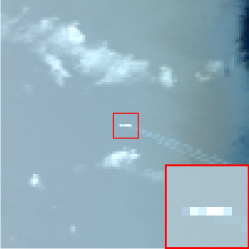
(a)

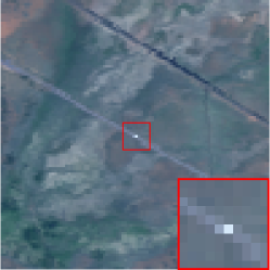
(b)

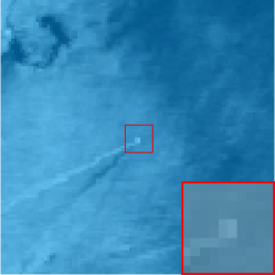
(c)

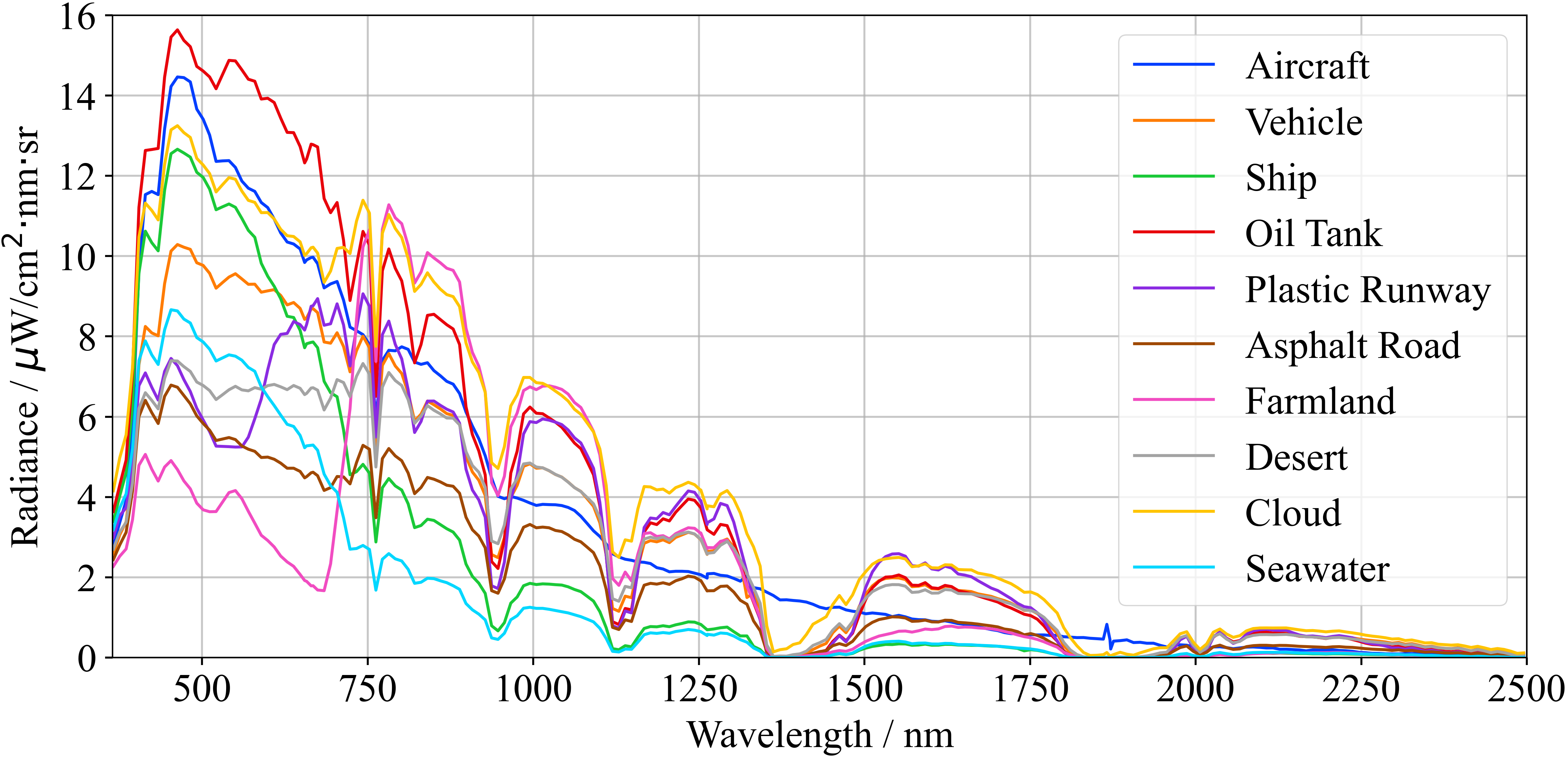
(d)

Figure 2: Real-world point objects in HSI collected by AVIRIS. (a) Aircraft. (b) Vehicle. (c) Ship. (d) Spectral radiance curves of several common objects.

Inspired by the current DETR-like detectors, we propose the first specialized network for hyperspectral point object detection, SpecDETR. We treat the spectral features of each pixel in the HSI as a token serving as the fundamental operation unit in Transformer [17]. Diverging from existing object detection networks, we bypass the backbone and directly employ a Transformer encoder to extract deep features from spectral tokens. Building upon the deformable attention module [18], we propose a local and global coordination (LGC) attention module, which efficiently samples local spectral features at the subpixel level while capturing global spectral features. Furthermore, based on the DINO [19] decoder, we design a concise decoder framework tailored for point object detection, integrating one-to-many label assignment and the end-to-end advantages of DETR. With the same attention operations and decoder layer number, our decoder achieves superior point object detection accuracy with fewer parameters than the DINO decoder. To advance the development of hyperspectral point object detection, we developed a hyperSpectral multi-class Point Object Detection dataset, termed SPOD. Using the SPOD dataset, we thoroughly evaluated the mainstream object detection networks and HTD methods. Our SpecDETR outperforms state-of-the-art (SOTA) object detection networks and current HTD methods on the SPOD dataset. The contributions of this paper can be summarized as follows:

1. We extend the hyperspectral point target detection to the point object detection and propose the first specialized hyperspectral point object detection network, SpecDETR.

2. We regard SpecDETR as a one-to-many set prediction problem and develop a concise and efficient DETR decoder framework that surpasses the current SOTA DETR decoder framework on point object detection.

3. We develop a hyperspectral point object detection benchmark and evaluate current object detection networks and HTD methods on the hyperspectral point object detection task for the first time.

The rest of this paper is organized as follows. Section II reviews the fields related to our work. Section III describes the details of SpecDETR. The datasets and experiments are presented in Section IV and Section V, respectively. Section VI presents supplementary experiments in the infrared small target detection task, followed by the conclusion in Section VII.

II Related Work

II-A Hyperspectral Detection

HTD aims to locate targets based on the spectral characteristics in HSIs [20]. Classic HTD methods can be categorized into matching methods [21], statistical analysis methods [10, 22, 23], and subspace-based methods [24, 25, 11]. While these methods demonstrate effective target-background separation in homogeneous scenarios, they have limitations in handling complex scenarios. In response to these limitations, machine learning-based techniques such as sparse representation [26, 27, 28, 29, 30, 31], kernel methods [32, 33, 34, 35, 12, 36], and deep learning [37, 38, 6, 6] have gained popularity due to their ability to handle complex data and achieve impressive performance. However, these methods are pixel-based and limited in their ability to represent features at the instance level.

Recently, object detection has been introduced to hyperspectral detection, showing promising results in fields such as camouflage object detection [39], vehicle detection [40, 41, 42], and methane gas detection [16]. For example, S2ADet [42] utilizes a two-stream network to extract spectral and spatial semantic information and aggregate them for object detection. However, these studies are designed for larger-sized objects and still rely on convolutional neural network (CNN) backbones for feature extraction, which are unsuitable for point object detection.

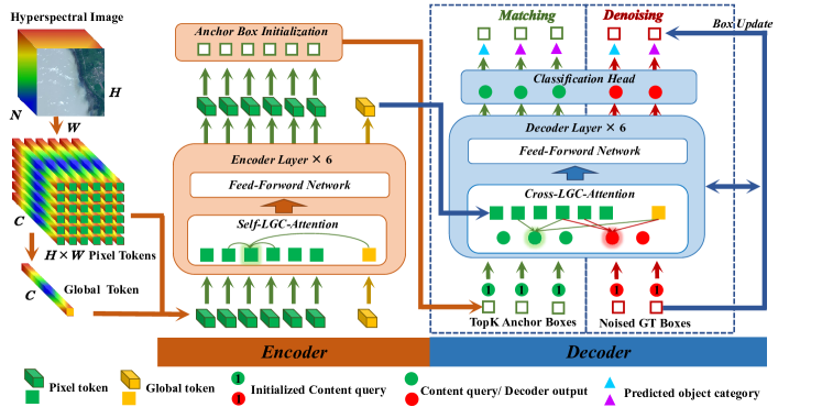
Figure 3: An overview of our SpecDETR. For clear visualization, we omit positional embedding and only display the classification prediction head of the final decoder layer.

II-B DETR

Carion et al. [15] proposed DETR, an end-to-end object detector based on Transformer [17], which reformulates object detection into a set prediction problem by employing an encoder-decoder architecture and one-to-one label assignment. Deformable DETR [18] introduces multi-scale features with deformable operations. Variants such as DAB-DETR [43] decompose the object query into the content query and positional query, incorporating explicit positional representations. Furthermore, DN-DETR [44], DINO [19], and GroupDETR [45] address the inefficiency of one-to-one matching by improving decoder queries. Our work demonstrates the superiority of the DETR architecture without the backbone in hyperspectral point object detection.

II-C Small Object Detection

In general object detection, small objects refer to limited-sized entities. For example, the COCO dataset [46] and SODA dataset [47] consider objects with a bounding box area equal to or smaller than 1024 pixels as small objects, which still contain certain texture and shape information. However, the point objects addressed in this paper have extremely limited texture and shape information. In recent years, significant progress has been made in infrared small target detection [48, 49], which can isolate point targets from single-band infrared images. However, these works primarily use saliency information to classify pixels into targets and backgrounds and cannot predict the categories of point targets. In this paper, we explore the feasibility of detecting multi-class point objects by using spectral information.

III Methodology

III-A Task Definition

Traditional HTD methods use a prior target spectral library to perform binary classification on pixels. Our work extends object detection to the hyperspectral point object detection task, aiming to achieve object-level detection of point targets. Our network learns object-level features on a set of training HSIs with bounding box (bbox) annotations of point objects. If annotations include category labels, the trained network can predict the categories of point objects. In contrast, the HTD methods always treat all target prior spectra as the same category and neglect classification ability. Additionally, hyperspectral classification methods [1] usually do not involve various background spectra not included in the prior spectral library. In contrast, hyperspectral point object detection requires identifying and rejecting these background spectra.

III-B Preliminary

Our SpecDETR is built upon DINO [19], a SOTA end-to-end object detector. DINO leverages the advancements of DAB-DETR [43], Deformable DETR [18], and DN-DETR [44]. It consists of a backbone, a Transformer encoder, a Transformer decoder, and multiple prediction heads. Following DAB-DETR, DINO decomposes decoder queries into content queries and positional queries. The positional queries are formulated as dynamic anchor boxes $\left(x,y,w,h\right)$ and refined step-by-step across decoder layers, where $x$ and $y$ are the center coordinates of the box and $w$ and $h$ are the width and height of the box. DINO employs mixed query initialization, where the initial anchor boxes (positional queries) are derived from the output of the encoder, while the content queries are learnable. DINO uses deformable attention [18] to reduce computational cost and employs a parameter update scheme called “look forward twice” to optimize decoder parameters. DN-DETR introduces denoising (DN) training by adding ground truth (GT) labels and boxes with noise into the Transformer decoder to stabilize bipartite matching during training. DINO proposed contrastive denoising (CDN) training by adding positive and negative samples of the same GT to avoid duplicate predictions.

III-C Overview

As shown in Fig. 3, our SpecDETR does not require the backbone part. It only consists of a multi-layer Transformer encoder, a multi-layer Transformer decoder, and multiple prediction heads. Given an HSI, we use a linear layer to transform the band number and treat each pixel as a token. Then, we feed them into the Transformer encoder to extract deep features. Anchor boxes based on the output of the multi-layer encoder are used as initial positional queries, while content queries are initialized as vectors of all ones. The initial anchors and content queries are sent into the multi-layer decoder and updated layer-by-layer. The outputs of SpecDETR consist of refined anchor boxes and classification results predicted by refined content features. During training, SpecDETR introduces an additional denoising branch alongside the original decoder branch, considered the matching branch. In response to the characteristics of point objects, we propose center-shifting contrastive denoising (CCDN) training to replace CDN training in DINO. While DETR treats detection as a one-to-one set prediction problem, SpecDETR views point object detection as a one-to-many set prediction problem. In the matching branch, we use a hybrid one-to-many label assigner instead of a Hungarian matching-based one-to-one label assignment in current DETR-like detectors. Based on the one-to-many matching, we simplify the decoder by removing cross-attention between content queries and initializing content queries as non-learnable vectors. Additionally, SpecDETR uses non-maximum suppression (NMS) to remove overlapping prediction boxes. Reintroducing one-to-many matching and NMS can enhance the end-to-end advantage of SpecDETR in point object detection. We will further elaborate on our improvement details in the following subsections, omitting details same to those of DINO [19].

III-D Data Tokenization

Given an HSI data cube $\bm{X}\in\mathbb{R}^{H\times W\times N}$, where $H$, $W$, and $N$ represent the width, height, and band number, we preprocess $\bm{X}$ before feeding it into the encoder by:

$$\bm{P}=LN\left(Linear\left(\frac{\bm{X}}{V}\right)\right),$$ (1)

where $Linear$ represents a linear layer, $LN$ represents a layer normalization layer [50], and $V$ is a constant. The output data cube $\bm{P}\in\mathbb{R}^{H\times W\times C}$ has a feature vector at each pixel position, serving as a pixel token for the following Transformer, where $C$ represents the dimension of tokens. Subsequently, a global token $\bm{g}$ is initialized by:

$$\bm{g}=\frac{1}{H\times W}\sum_{H\times W}^{i=1}{\bm{p}_{i}},$$ (2)

where $\bm{p}_{i}$ represents the $i-$th pixel token.

The 8-bit quantized RGB images are typically Z-score normalized on each band before being fed into a neural network. However, HSIs have higher quantization bits and more bands, and each band has different data distributions. Some bands have minor standard deviations, leading to increased values after Z-score normalization, which can affect network convergence. Therefore, in Eq. (1), we normalize the radiance values or digital number values on all bands of the HSI by dividing them by the same constant $V$. The choice of $V$ is not strict; it should ensure that most values in the normalized HSI are smaller than 1. We refer to $V$ as the normalization constant.

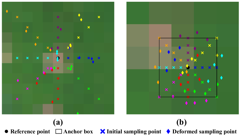
Figure 4: Sampling points of LGC attention modules with 8 attention heads and 4 points per attention head on the Avon dataset [51]. (a) Self-attention modules in the encoder. (b) Cross-attention modules in the decoder. Different colors represent different attention heads.

III-E Local and Global Coordination Attention Module

Inspired by deformable convolution [52], the deformable attention module [18] only uses a small set of sampling points around a reference point to calculate the multi-head attention [17] and solves the high computational complexity and slow convergence in DETR [15].

In HSIs, the features of point objects mainly lie in their spectra. Therefore, the feature extraction for point objects should primarily focus on a small number of pixels around the objects. We employ the deformable attention module to adaptively aggregate local neighborhood features around the reference points in the feature maps $\bm{P}$. Given a query element $\bm{q}$ and its reference point $\bm{r}$, its deformable attention feature in $\bm{P}$ is calculated by

$$Attn\left(\bm{P},\bm{q}\right)=\sum_{m=1}^{M}{\bm{W}_{m}\sum_{k=1}^{K}{\bm{W}_{m}^{\prime}A_{mk}}f\left(\bm{P},\bm{r}+\varDelta\bm{r}_{mk}\right)},$$ (3)

where $m$ indexs the attention heads, $k$ indexs the sampling pionts, $M$ is the attention head number, and $K$ is the sampled key number. $\bm{W}_{m}$ and $\bm{W}_{m}^{\prime}$ are learnable weights. $\varDelta\bm{r}_{mk}$ is the sampling piont offset of the $k$-th sampling piont in the $m$-th attention head, and $A_{mk}$ is the attention weight of the sampling piont $\bm{r}+\varDelta\bm{r}_{mk}$. $\varDelta\bm{r}_{mk}$ and $A_{mk}$ are both generated by linearly projecting $\bm{q}$. $f\left(\bm{P},\bm{r}^{\prime}\right)$ is the sampled key corresponding to the shifted sampling point $\bm{r}^{\prime}$, which is obtained through bilinear interpolation on $\bm{P}$:

$$f\left(\bm{P},\bm{r}^{\prime}\right)=\sum_{i=1}^{4}{\varepsilon_{i}\bm{p}_{i}^{\prime}},$$ (4)

where $\bm{p}_{1}^{\prime}$, $\bm{p}_{2}^{\prime}$, $\bm{p}_{3}^{\prime}$, and $\bm{p}_{4}^{\prime}$ are the four pixel tokens closest to $\bm{r}^{\prime}$, and $\varepsilon_{i}$ represents the weights based on positional distance, satisfying $\varepsilon_{i}>0$ and $\sum_{i=1}^{4}{\varepsilon_{i}}=1$. According to the linear mixing model (LMM) [53], $f\left(\bm{P},\bm{r}^{\prime}\right)$ can be viewed as the mixed spectral feature of the four pixel tokens. Through bilinear interpolation, discrete $\bm{P}$ is transformed into a spectral feature space that is continuous in positional dimensions, allowing the attention operation to capture features with subpixel granularity.

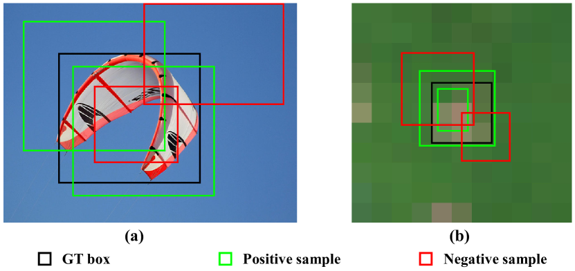
Figure 5: Illustration of positive and negative positional queries of CDN and CCDN training. (a) CDN. (b) CCDN.

For traditional hyperspectral anomaly detection methods and HTD methods [20], background spectra are necessary inputs. These traditional methods use background spectral information as the reference to search target spectra. However, the deformable attention module extracts local spectral features from local sampling points around the reference point, and the positions of sampling points are not fixed. Consequently, the background spectral features extracted by the deformable attention module are unstable. Hence, we propose a local and global coordination (LGC) attention module, which incorporates the global token $\bm{g}$ as a key element into Eq. (3), achieving the aggregation of global and local spectral features and ensuring stable background spectral information input. Eq. (3) is rewritten as:

$$LGCAttn\left(\bm{P},\bm{g},\bm{q}\right)=$$ (5)

$$\sum_{m=1}^{M}{\bm{W}_{m}\sum_{k=1}^{K}{\bm{W}_{m}^{\prime}\left(A_{mk}f\left(\bm{P},\bm{r}+\varDelta\bm{r}_{mk}\right)+A_{gmk}\bm{g}\right)}},$$

where $A_{gmk}$ is the attention weight of $\bm{g}$.

In each encoder layer of SpecDETR, the global token and pixel tokens serve not only as key elements in the attention module but also as query elements. When a pixel token is used as a query, its reference point is the center of the corresponding pixel. As shown in Fig. 4(a), the attention heads marked in light blue primarily focus on the feature of the query itself, while other attention heads focus on different neighborhood features of the query. The reference point of the global token is the midpoint of $\bm{P}$. After each encoder layer, the global token and pixel tokens are updated with the output values.

In each decoder layer of SpecDETR, the updated global token and pixel tokens from the final encoder layer act as key elements, with the content queries serving as query elements. As shown in Fig. 4(b), the sampling points of a content query are initially constrained within the corresponding anchor box, while deformed sampling points can focus on the internal and edge features of the anchor box.

III-F Hybrid Label Assigner

DETR [15] treats object detection as a one-to-one set prediction problem, using the Hungarian matching to assign only one object query to each GT box, eliminating the need for NMS whose IoU threshold requires manual selection based on the overall object overlap situation in the data. Indeed, current DETR-like detectors still cannot completely avoid redundant predictions. Therefore, SpecDETR does not reject NMS and treats hyperspectral point object detection as a one-to-many set prediction problem. Specifically, we replace the Hungarian matching with a one-to-many label assigner in the matching branch. We observed that the overlap between anchor boxes and GT boxes is dynamic during training. The initialized anchor boxes from the encoder gradually align with the GT boxes as the network converges, and each decoder layer refines the input anchor boxes. Hence, we propose a hybrid label assigner consisting of forced matching and dynamic matching to improve the quality of assigned anchor boxes as the network converges.

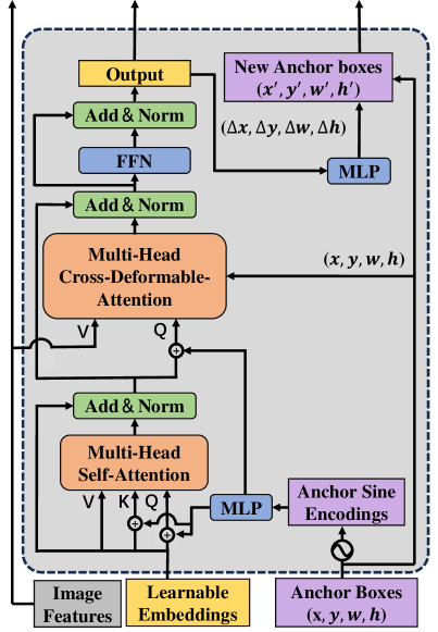
(a)

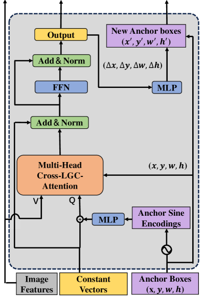
(b)

Figure 6: Comparison of decoder layer structures. (a) DINO. (b) SpecDETR. Only the first layer is illustrated. The structure of the remaining layers is identical to that of the first layer, while the content queries are the output of the preceding layers.

Forced Matching. We first employ the Hungarian matching in DETR [15] to assign a positive sample to each GT box based on class prediction and the similarity between anchor boxes and GT boxes. We forcefully assign positive samples to GT boxes without highly overlapping anchor boxes to enable the network to explore the features of hard samples.

Dynamic Matching. After the forced matching, we use the Max IoU assigner [13] to further allocate positive samples among the remaining anchor boxes. In addition to the IoU threshold, we introduce a number threshold $T$. If a GT box is assigned to more than $T$ anchor boxes, we retain only the top $T$ anchor boxes with the highest IoU as positive samples.

III-G Center-Shifting Contrastive DeNoising Training

DN-DETR introduces a DeNoising (DN) training branch in the decoder to stabilize training and accelerate convergence. DINO improved DN training to Contrastive DeNoising (CDN) training, incorporating negative queries to reject useless anchors. CDN generates positive and negative positional queries by adding two levels of noise (position offsets) to the corners of the GT boxes. However, CDN is designed for one-to-one matching, where the range of negative queries includes the positive queries, as shown in Fig. 5(a). Negative samples with high overlap with GT boxes can disrupt classification in the case of one-to-many matching. Therefore, we adopt the query generation method of DN [44], consisting of center shifting and box scaling steps controlled by hyperparameters $\tau_{1}$ and $\tau_{2}$, with $\tau_{1}>0$ and $\tau_{2}>0$. Our denoising approach adds two levels of shifting to the centers of the GT boxes to generate positive and negative positional queries, termed as Center-Shifting Contrastive DeNoising (CCDN).

Center Shifting. Given a GT box $\left(x,y,w,h\right)$, random noises $\left(n_{x},n_{y}\right)$ are added to the center$\left(x,y\right)$. For positive queries, the noise satisfies $-0.5\tau_{1}w<n_{x}<0.5\tau_{1}w$ and $-0.5\tau_{1}h<n_{y}<0.5\tau_{1}h$. For negative samples, $n_{x}$ is randomly sampled within the range $\left[-\tau_{1}w,-0.5\tau_{1}w\right]\cup\left[0.5\tau_{1}w,\tau_{1}w\right]$, and $n_{y}$ is randomly sampled within the range $\left[-\tau_{1}h,-0.5\tau_{1}h\right]\cup\left[0.5\tau_{1}h,\tau_{1}h\right]$.

Box Scaling. Regardless of positive or negative queries, the width and height are randomly sampled within the ranges $[\min\left(0,w-\tau_{2}w\right),w+\tau_{2}w]$ and $[\min\left(0,h-\tau_{2}h\right),h+\tau_{2}h]$, respectively.

(a)

(b)

(c)

(d)

(e)

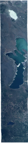
(f)

(g)

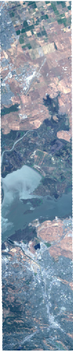
(h)

Figure 7: Partial regions of AVIRIS flight lines used to construct the SPOD dataset. (a)-(d) The flight line f180601t01p00r06 for training data. (e)-(h) The flight line f180601t01p00r10 for test data.

III-H Decoder Simplification

From the perspective of a one-to-many set prediction problem, we can optimize both the label assigner and denoising training approach while further simplifying the structure of the decoder. As shown in Fig. 6, compared to the decoder in DINO derived from Deformable DETR, our decoder removes the self-attention computation between content queries. The self-attention module helps reject redundant boxes and is unnecessary for our SpecDETR. Additionally, we initialize the content queries with vectors of all ones rather than the index embeddings used in DINO.

IV Datasets

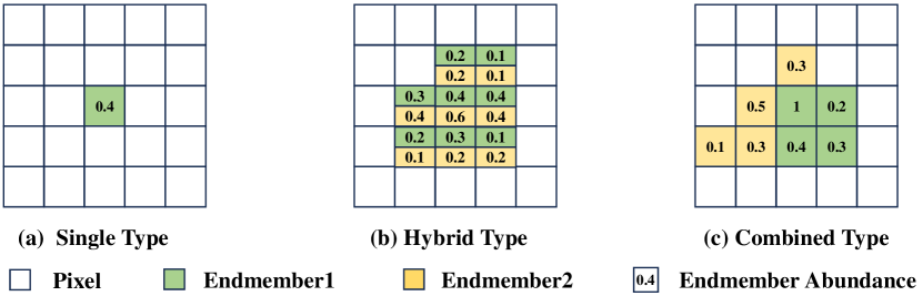
Figure 8: Diagrams of the three types of object templates on the SPOD dataset.

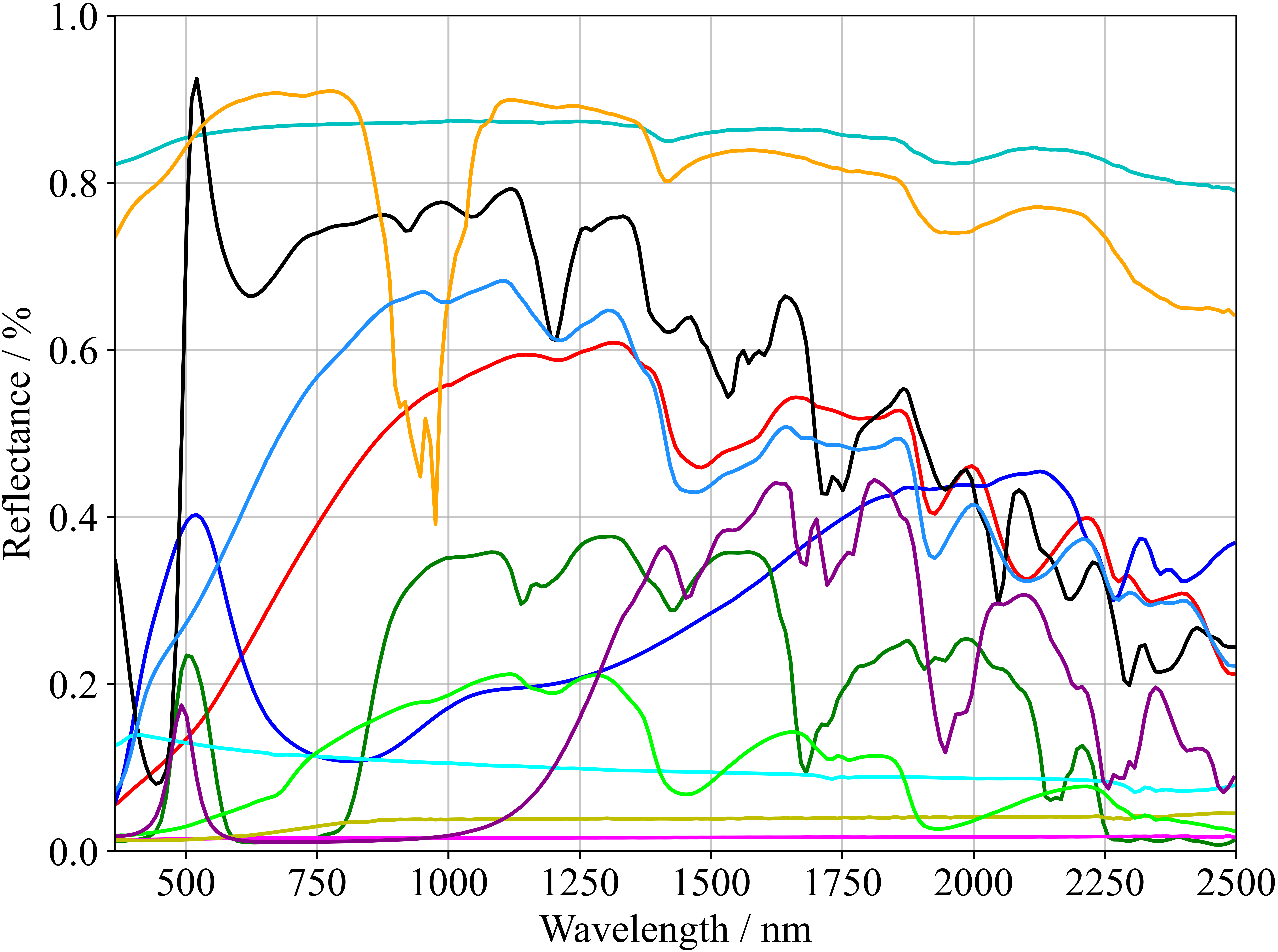
(a)

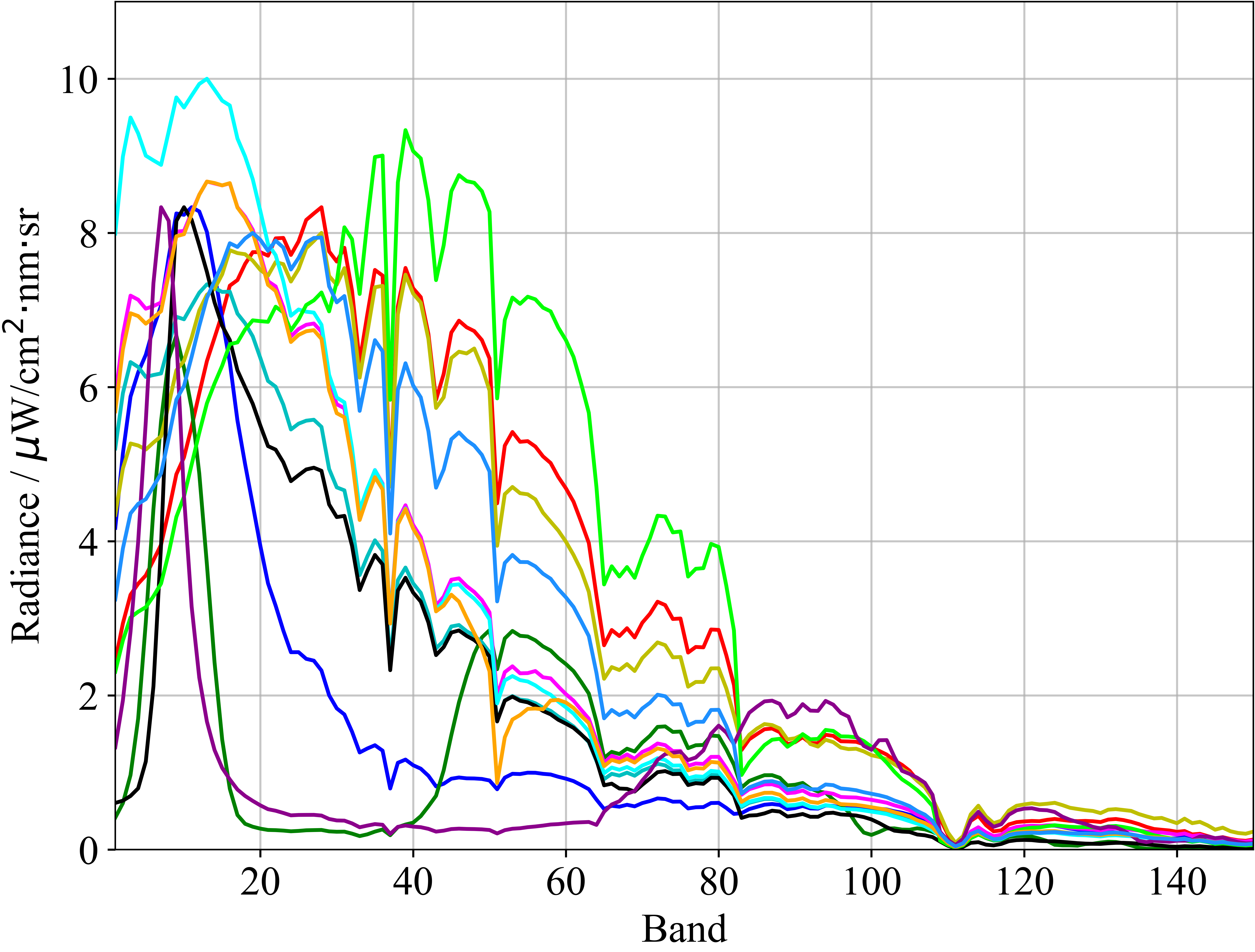
(b)

(c)

Figure 9: Spectral curves of different endmembers. (a) Reflectance curves. (b) Baseline radiance curves. (c) Radiance curves after adding noise.

TABLE I: The object simulation setup on the SPOD dataset.

Name	Type	Endmember	Pixel	Maximum	Training	Test
		Components	Number	Abundance	Samples	Samples
C1	Single	Cardboard	1	0.05-0.2	122	686
C2	Single	Malachite	1	0.05-0.2	118	674
C3	Single	Fiberglass	1-2	0.2-1	136	633
C4	Single	NickelPowder	3-5	0.2-1	120	664
C5	Single	LutetiumOxide	3-5	0.2-1	108	688
		Kerogen,
C6	Hybrid	NylonWebbing	6-10	0.2-1	122	669
		PlasticSheet,
C7	Combined	OiledMarshPlant	6-10	0.2-1	106	686
		Verdigris,
		YtterbiumOxide,
C8	Combined	WoodBeam	11-16	0.2-1	123	629

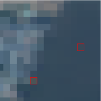
(a) C1

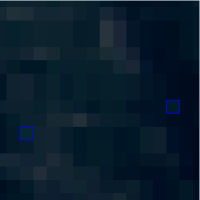
(b) C2

(c) C3

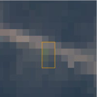
(d) C4

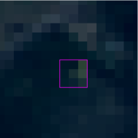
(e) C5

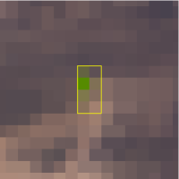
(f) C6

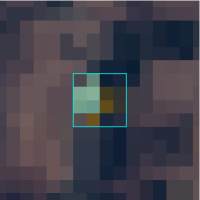
(g) C7

(h) C8

Figure 10: Examples of objects on the SPOD dataset on pseudo-color images.

This section will introduce our simulated dataset and a public hyperspectral target detection dataset.

IV-A The SPOD Dataset

Due to the spectral mixing phenomenon, acquiring a large number of high-quality manually annotated point objects is extremely challenging. Therefore, we develop a simulated high-spectral multi-class point object detection benchmark based on observed real-world patterns to evaluate the accuracy performance of various methods in point object detection. As shown in Fig. 7, we selected two flight lines captured by the AVIRIS sensor over California and Nevada, covering 21,000 $km^{2}$ of the Earth’s surface with significant geographic variation. One flight line provides 150 128$\times$128 training background images, while the other provides 500 128$\times$128 testing background images. After removing the atmospheric absorption bands, we retained 150 bands with the band IDs [8-57, 66-79, 86-103, 123-145, 146-149, 173-214].

We first generate object abundance templates. Then, following the LMM [53], we injecte object endmember spectra into background HSIs. Spectra of the same material are affected by various factors such as illumination, so we analyze the spectral local variation property and wide-area variation property of water area in AVIRIS images, using them to generate endmember spectra.

Object Template Generation: We randomly choose the pixel number $N_{P}$ and the maximum abundance $M_{A}$ from the specified ranges. Then, a clustered random combination of $N_{P}$ pixels is generated. Subsequently, $N_{P}$ object abundances are randomly generated within the range$[0.01,M_{A}]$ and distributed from the center to the edges in descending order. If all the four neighboring pixels of a pixel are object pixels, its abundance is set to 1. If all pixel abundances are smaller than $M_{A}$, the abundance of the central pixel is set to $M_{A}$. As shown in Fig. 8, in addition to single-spectral objects, we designed two types of multi-spectral object templates: hybrid objects, where each pixel contains two or more endmember spectra, and combined objects, which can be considered as spatial concatenations of multiple single-spectral objects.

Endmember Spectral Generation: As shown in Fig. 8(a), we select 12 types of artificial object spectral reflectance curves $\bm{r}_{t}$ from the USGS spectral library [54]. Based on the reflectance curve $\bm{r}_{t}$ of seawater and an average radiance curve $\bm{s}_{w}$ of a seawater region in the AVIRIS data, $\bm{r}_{t}$ is converted into simulated endmember baseline reference spectrum $\bm{s}_{t}$ by:

$$\bm{s}_{t}=\frac{M_{t}}{\max\left(\frac{\bm{r}_{t}}{\bm{r}_{w}}\circ\bm{s}_{w}\right)}\frac{\bm{r}_{t}}{\bm{r}_{w}}\circ\bm{s}_{w},$$ (6)

where $\circ$ denotes the Hadamard product, ${M_{t}}$ is the correction to ensure that the numerical range of the simulated endmember baseline reference spectra is close to the background HSIs, and ${M_{t}}$ has slight differences for different endmember. Fig. 9(b) shows the transformed simulated endmember reference spectra. Then, we generate endmember spectra by adding noise into reference spectra based on the statistical variation properties of water area spectra in AVIIS data, as shown in Fig. 9(c). Spectra of the same object only exhibit the local fluctuation property, while different objects exhibit the wide-area variation property. Further details can be found in the Supplementary Material.

As shown in Table I, we set 8 types of objects, where C1 and C2 are subpixel objects with abundances smaller than 0.2, and C5-C8 are multi-spectral objects. Examples of each object type on pseudo-color images are shown in Fig. 10, where C1 and C2 are barely perceptible to the human eye. To increase the challenge, we average every 5 adjacent bands, reducing the 150 bands to 30 bands to reduce spectral information.

IV-B The Avon Dataset

The Avon dataset was collected by a ProSpecTIR-VS sensor during the SHARE 2012 data campaign [51]. It has a spatial resolution of 1m and a spectral resolution of 5nm, with 360 bands between 400-2450nm. As shown in Fig. 11, we crop a test image of size 128$\times$128, which contains 12 blue tarps and 12 brown tarps. The spectra of the edge pixels of the tarps are a compromise between the pure tarp spectra and the grass background spectrum. Between 800-1200nm, the spectrum of brown tarps is similar to that of the soin background. We use pure and unmixed tarp spectra as prior spectra for target detection and manually select pixels from detection maps to form the per-pixel annotations shown in Fig. 11(c). Additionally, we use the pure blue tarp spectrum and brown tarp spectrum from Fig. 11(d) as endmember spectra and cut background images from another fight line collected by the SHARE 2012, generating 150 training images with 1500 simulated blue tarps and 1500 simulated brown tarps.

V Experiments

V-A Comparison Experiments on the SPOD Dataset

V-A1 Implementation Details

We use the MMDetection project [55] to implement SpecDETR and evaluate object networks provided by MMDetection on the SPOD Dataset. For SpecDETR, the parameters $\tau_{1}$ and $\tau_{2}$ of CCDN are set to 0.5 and 1.5, respectively, and the number of DN queries is fixed at 200 pairs. For the dynamic matching in the hybrid label assigner, the IoU threshold is set to 0.95, and the number threshold $T$ is set to 9. The learning rate is initialized as 0.001, and it is multiplied by 0.1 at the 20th, 30th, and 90th epochs with the setting of 24, 36, and 100 training epochs, respectively. During the inference stage, we select the top 300 predicted boxes with the highest confidence scores for each image and then use NMS to remove redundant boxes. The IoU threshold for NMS is set to 0.01, meaning that the final output predicted boxes are considered non-overlapping. The remaining parameters are set to the same values as DINO. For other evaluated networks, we upscale the input HSIs by a factor of 4 by replicating each pixel 16 times. The input channels of these networks are adjusted from 3 to the band number of the input HSIs. The training epoch number is set to 100, while the remaining parameters are set to their defaults. All the networks are trained with a batch size of 4 on an RTX 3090 GPU.

(a)

(b)

(c)

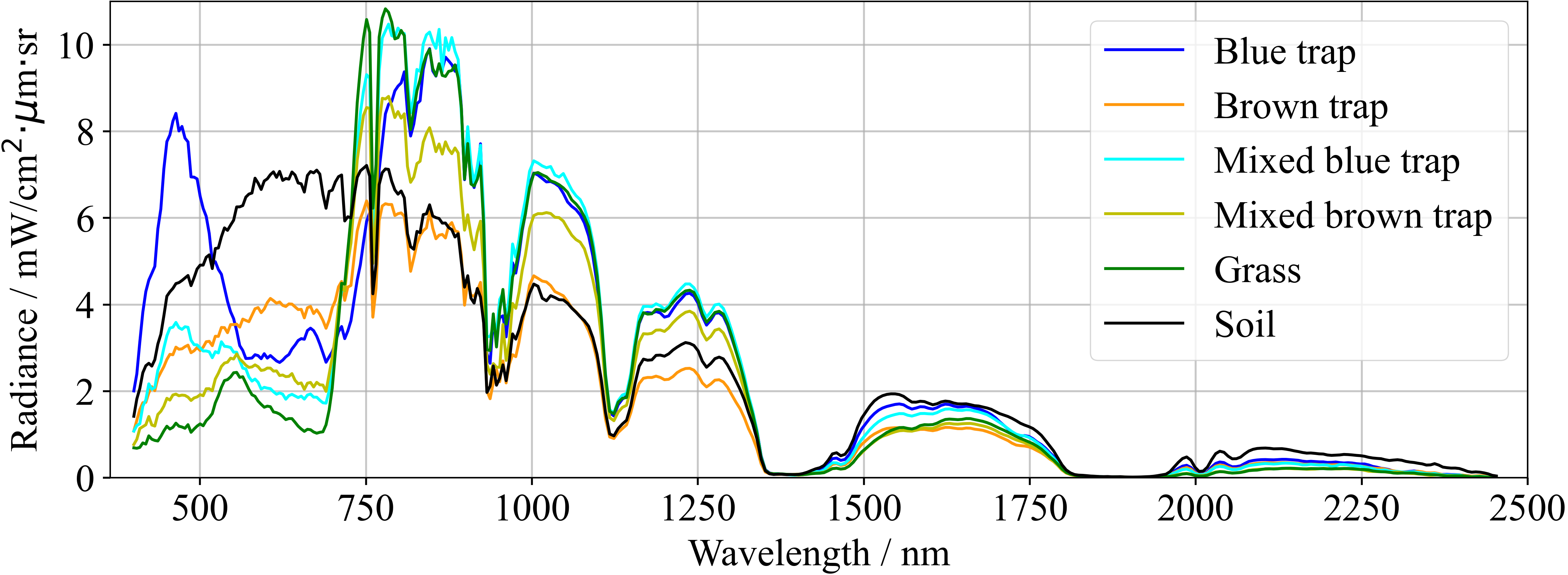
(d)

Figure 11: The Avon dataset. (a) Pseudo-color image. (b) Zoomed-in image of the surrounding area of objects. (c) GT. (d) Radiance spectral curves of objects and background.

We also evaluate traditional HTD methods [24, 10, 25, 21, 23, 56, 35, 29, 30, 11, 12, 36]. For each type of object, we provide 20 prior spectral curves. The output results of these methods are detection score maps. We perform binary segmentation on the score maps and then transform the segmentation maps into predicted boxes, where the confidence score of each box is the maximum detection score within that box. The segmentation threshold $t$ is calculated as follows:

$$t=\mu_{t}+\lambda\sigma_{t},$$ (7)

where $\mu_{t}$ and $\sigma_{t}$ are the mean and standard deviation of all scores, respectively, and $\lambda$ is the segmentation factor. For each HTD method, we traverse $\lambda$ from 1 to 15 to determine $\lambda$ that corresponds to the maximum mAP across all categories.

V-A2 Evaluation Metrics

We follow the standard COCO evaluation [46] and report the average precision (AP) of each class and mean AP (mAP) and mean average recall (mAR) across all classes. In addition, we also report the $\text{mAP}_{\text{25}}$ and mean recall $\text{mRe}_{\text{25}}$ at an IoU threshold of 0.25, which sufficiently demonstrate the localization ability for point objects. For HTD methods, we also compute the area under the ROC curve (AUC) [57] for the score maps and the IoU for the segmentation maps, and report the mean AUC (mAUC) and IoU (mIoU) across all categories.

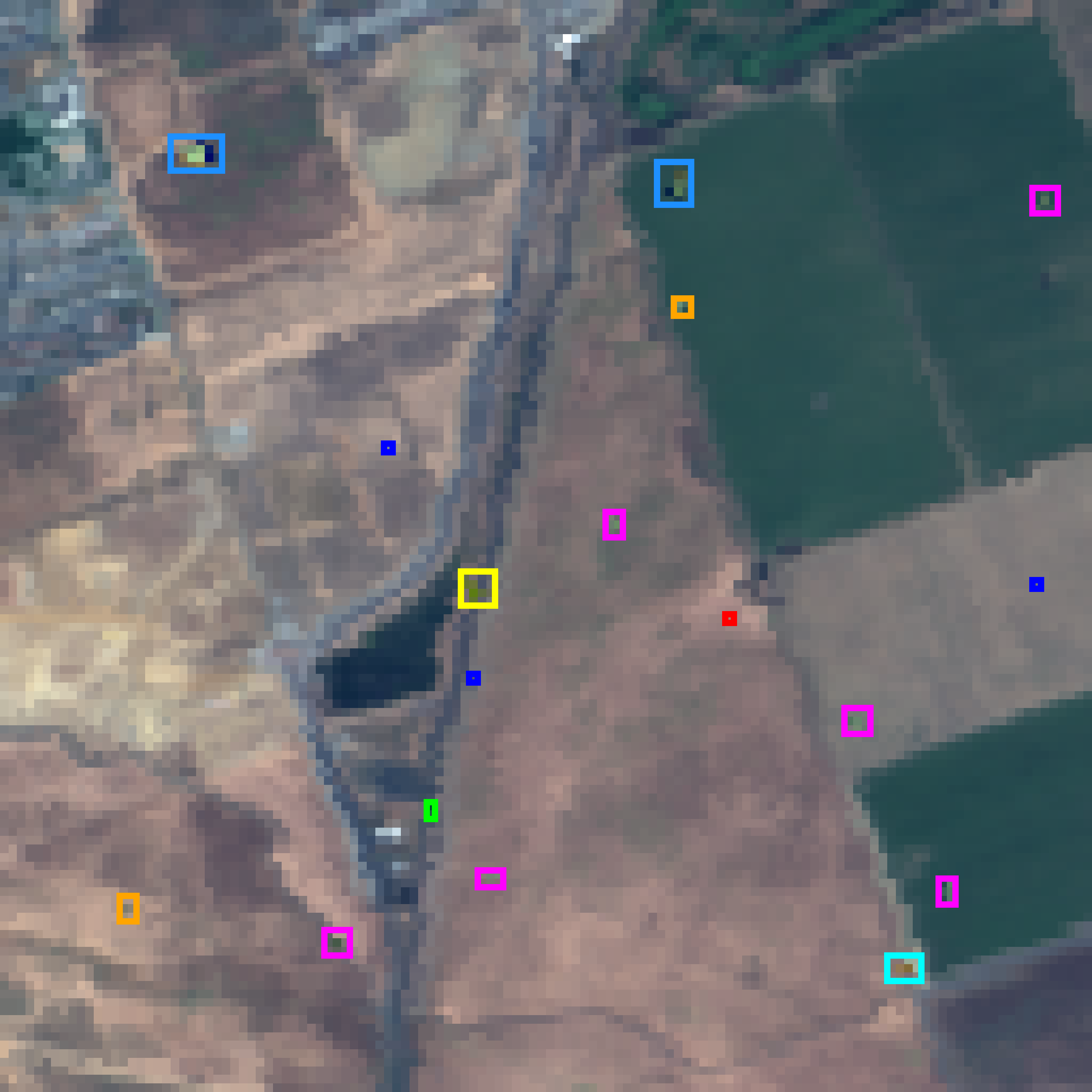
(a) GT

(b) SpecDETR

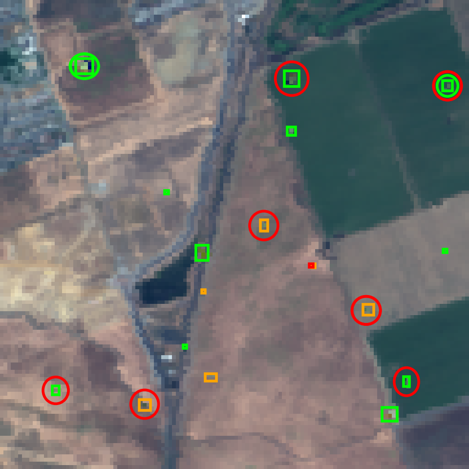
(c) DeformableDETR

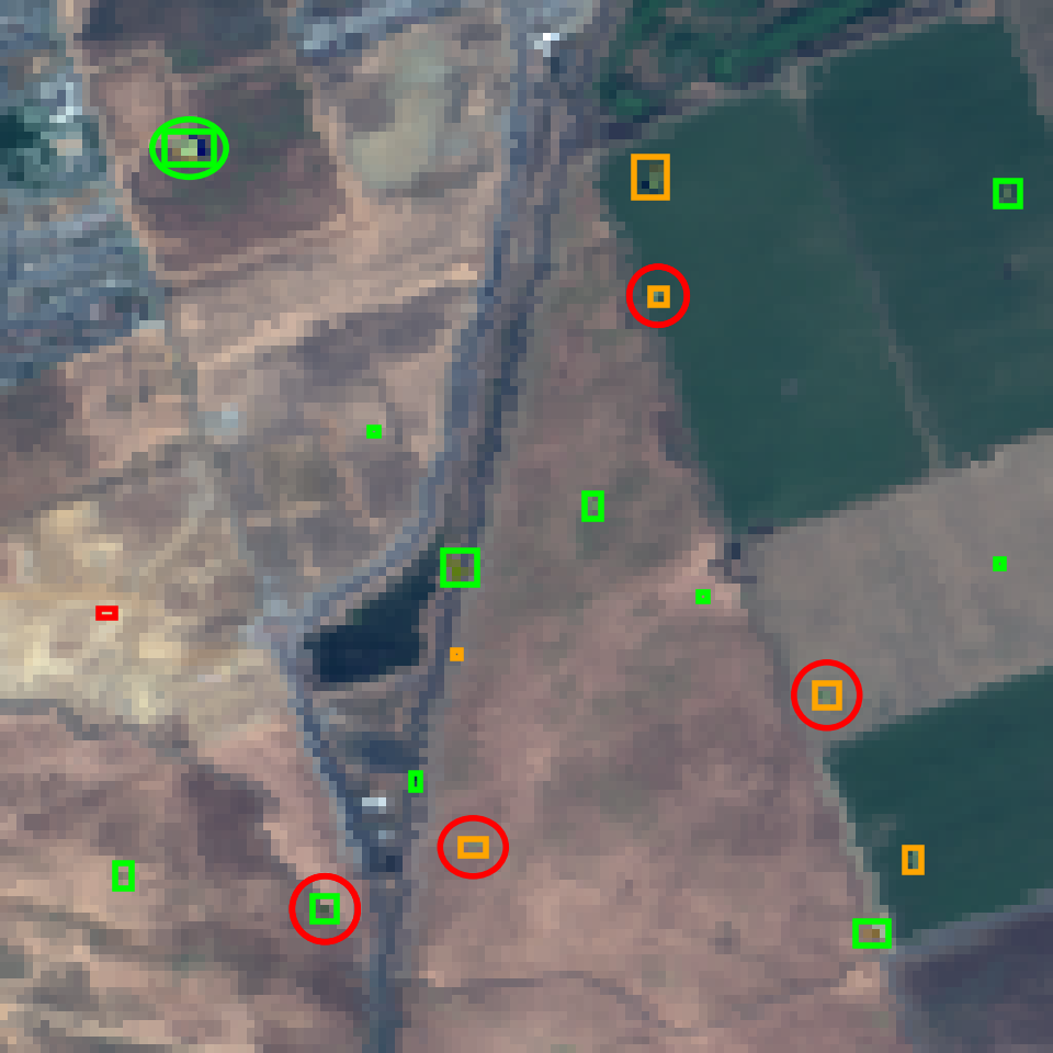
(d) DINO with Swin

Figure 12: Visualization results of SpecDETR and other DETR-like detectors. (a) The color of GT boxes is consistent with the meaning in Fig. 10. (b)-(d) Only predictions with a confidence score greater than 0.2 are shown. Green boxes are correct predictions that have an IoU greater than 0.25 with GT, red boxes are false alarms, yellow boxes are missed objects, green circles are redundant correct predictions, and red circles are predictions with incorrect categories.

TABLE II: Performance comparison of SpecDETR and object detection networks on the SPOD dataset. Size $\times$4 indicates that the input images are enlarged by a factor of 4, while $\times$1 represents the original size.

Detector	Bakebone	Epochs	Size	mAP$\uparrow$	$\text{mAP}_{\text{25}}$$\uparrow$	mAR$\uparrow$	$\text{mRe}_{\text{25}}$$\uparrow$	$\text{AP}_{\text{C1}}$$\uparrow$	$\text{AP}_{\text{C2}}$$\uparrow$	$\text{AP}_{\text{C3}}$$\uparrow$	$\text{AP}_{\text{C4}}$$\uparrow$	$\text{AP}_{\text{C5}}$$\uparrow$	$\text{AP}_{\text{C6}}$$\uparrow$	$\text{AP}_{\text{C7}}$$\uparrow$	$\text{AP}_{\text{C8}}$$\uparrow$	Params$\downarrow$
Faster R-CNN[13]	ResNet50[58]	100	$\times$4	0.197	0.377	0.245	0.419	0.000	0.000	0.000	0.035	0.026	0.537	0.430	0.550	41.5M
Faster R-CNN[13]	RegNetX[59]	100	$\times$4	0.227	0.379	0.267	0.399	0.000	0.000	0.000	0.042	0.043	0.631	0.522	0.578	31.6M
Faster R-CNN[13]	ResNeSt50[60]	100	$\times$4	0.246	0.316	0.269	0.319	0.000	0.000	0.000	0.008	0.003	0.644	0.564	0.747	44.6M
Faster R-CNN[13]	ResNeXt101[61]	100	$\times$4	0.220	0.368	0.253	0.376	0.000	0.000	0.000	0.016	0.010	0.618	0.518	0.596	99.4M
Faster R-CNN[13]	HRNet[62]	100	$\times$4	0.320	0.404	0.364	0.434	0.000	0.000	0.000	0.107	0.076	0.849	0.731	0.793	63.2M
TOOD[63]	ResNeXt101[61]	100	$\times$4	0.304	0.464	0.401	0.570	0.000	0.000	0.000	0.181	0.194	0.743	0.648	0.663	97.7M
CentripetalNet[64]	HourglassNet104[65]	100	$\times$4	0.695	0.829	0.840	0.956	0.831	0.888	0.915	0.373	0.367	0.810	0.655	0.725	205.9M
CornerNet[66]	HourglassNet104[65]	100	$\times$4	0.626	0.736	0.855	0.969	0.797	0.751	0.855	0.328	0.308	0.768	0.554	0.644	201.1M
RepPoints[67]	ResNet50[58]	100	$\times$4	0.207	0.691	0.346	0.934	0.043	0.143	0.269	0.071	0.073	0.372	0.265	0.417	36.9M
RepPoints[67]	ResNeXt101[61]	100	$\times$4	0.485	0.806	0.635	0.961	0.373	0.561	0.632	0.242	0.253	0.658	0.508	0.649	58.1M
RetinaNet[68]	EfficientNet[69]	100	$\times$4	0.462	0.836	0.611	0.971	0.566	0.602	0.530	0.182	0.210	0.566	0.471	0.569	18.5M
RetinaNet[68]	PVTv2-B3[70]	100	$\times$4	0.426	0.757	0.650	0.987	0.356	0.478	0.458	0.209	0.232	0.563	0.470	0.644	52.4M
DeformableDETR[18]	ResNet50[58]	100	$\times$4	0.231	0.692	0.385	0.883	0.230	0.316	0.234	0.077	0.070	0.289	0.238	0.395	40.2M
DINO[19]	ResNet50[58]	100	$\times$4	0.168	0.491	0.368	0.763	0.020	0.047	0.277	0.080	0.064	0.286	0.213	0.360	41.6M
DINO[19]	Swin-L[71]	100	$\times$4	0.757	0.852	0.909	0.983	0.915	0.912	0.951	0.483	0.497	0.847	0.728	0.721	218.3M
SpecDETR	-	100	$\times$1	0.856	0.938	0.897	0.955	0.963	0.969	0.970	0.698	0.648	0.905	0.844	0.850	16.1M

TABLE III: Performance comparison of SpecDETR and HTD methods on the SPOD dataset.

Method	$\lambda$	mAUC$\uparrow$	mIoU$\uparrow$	mAP$\uparrow$	$\text{mAP}_{\text{25}}$$\uparrow$	mAR$\uparrow$	$\text{mRe}_{\text{25}}$$\uparrow$	$\text{AP}_{\text{C1}}$$\uparrow$	$\text{AP}_{\text{C2}}$$\uparrow$	$\text{AP}_{\text{C3}}$$\uparrow$	$\text{AP}_{\text{C4}}$$\uparrow$	$\text{AP}_{\text{C5}}$$\uparrow$	$\text{AP}_{\text{C6}}$$\uparrow$	$\text{AP}_{\text{C7}}$$\uparrow$	$\text{AP}_{\text{C8}}$$\uparrow$
ASD[24]	2	0.991	0.067	0.025	0.031	0.638	0.749	0.000	0.000	0.089	0.012	0.012	0.027	0.036	0.028
CEM[10]	14	0.981	0.140	0.034	0.078	0.185	0.452	0.001	0.059	0.204	0.001	0.001	0.006	0.001	0.000
OSP[25]	11	0.969	0.137	0.024	0.078	0.220	0.558	0.005	0.042	0.133	0.002	0.001	0.009	0.005	0.000
SMF[21]	5	0.904	0.032	0.003	0.016	0.067	0.260	0.000	0.000	0.024	0.000	0.000	0.000	0.000	0.000
HSS[23]	3	0.799	0.296	0.103	0.278	0.356	0.592	0.000	0.000	0.000	0.065	0.072	0.297	0.109	0.286
MSD[56]	3	0.982	0.483	0.224	0.490	0.547	0.882	0.069	0.241	0.743	0.093	0.075	0.233	0.082	0.259
KMSD[35]	9	0.965	0.321	0.110	0.277	0.376	0.692	0.010	0.006	0.543	0.043	0.041	0.129	0.049	0.058
SRBBH[29]	3	0.800	0.127	0.029	0.067	0.372	0.598	0.000	0.000	0.000	0.038	0.029	0.055	0.049	0.063
CSRBBH[30]	8	0.977	0.155	0.043	0.110	0.281	0.632	0.030	0.016	0.260	0.006	0.004	0.008	0.010	0.008
TCIMF[11]	5	0.975	0.071	0.017	0.057	0.334	0.729	0.004	0.000	0.082	0.008	0.005	0.013	0.015	0.011
KTCIMF[12]	2	0.863	0.007	0.002	0.010	0.260	0.644	0.000	0.000	0.004	0.003	0.004	0.002	0.001	0.002
SVMCK[36]	4	0.875	0.023	0.005	0.026	0.201	0.574	0.000	0.000	0.016	0.004	0.003	0.005	0.004	0.007
SpecDETR	-	-	-	0.856	0.938	0.897	0.955	0.963	0.969	0.970	0.698	0.648	0.905	0.844	0.850

V-A3 Result Analysis

Table II provides the performance comparison between SpecDETR and the networks that are effective in point object detection. SpecDETR achieves the highest mAP of 0.856 after 100 epochs among all compared networks. Due to the removal of the backbone part, SpecDETR has a parameter of only 16.1M. SpecDETR exhibits remarkable detection capability for subpixel objects and achieves $\text{AP}_{\text{C1}}$, $\text{AP}_{\text{C2}}$, and $\text{AP}_{\text{C3}}$ of 0.963, 0.969, and 0.97, respectively. Fig. 12 presents the detection results of SpecDETR, DeformableDETR, and DINO on a test HSI. Despite being end-to-end detectors, both DeformableDETR and DINO still exhibit redundant correct predictions, indicating the necessity of reintroducing NMS in SpecDETR. SpecDETR produces incorrect category predictions for C4 and C5, resulting in lower $\text{AP}_{\text{C4}}$ and $\text{AP}_{\text{C5}}$. Compared to other objects, C4 and C5 pose more challenging category prediction for SpecDETR, leading to lower $\text{AP}_{\text{C4}}$ and $\text{AP}_{\text{C5}}$.

We also observe that those backbones that can offer high-resolution shallow features are more valuable in point object detection. Followed by Faster R-CNN, HRNet, which achieves multi-scale feature interaction, outperforms ResNeXt. CentripetalNet and CornerNet with HourglassNet achieve 0.626 mAP and 0.691 mAP, respectively.

Moreover, the backbones based on Visual Transformer can also provide valuable features of point objects in HSIs. As shown in Table III, SpecDETR outperforms the compared HTD methods in detection accuracy. AUC, the classic evaluation metric for HTD, fails to reflect instance-level object detection performance. While ASD achieves the highest mAUC of 0.991, it only achieves a mIoU of 0.067 and an mAP of 0.025.

V-B Impact of Spectral Information on Point Object Detection

In the experiments in Sec. V-A, we performed spectral downsampling on the SPOD dataset, effectively simulating multispectral images with 30 bands from HSIs with 150 bands. The full width at half maximum (FWHM) on the 30-band SPOD dataset is equivalent to 50nm. There are differences in spectral information for hyperspectral and aligned multispectral images, but processing technology is consistent. We employ the same downsampling way to sequentially obtain versions of the SPOD dataset with 1, 2, 3, 5, 10, 15, 20, 25, 50, and 100 bands to evaluate the impact of spectral information on the point object detection performance of SpecDETR. As shown in Table IV, SpecDETR demonstrates improved detection performance for point objects with increased spectral information. SpecDETR fails to detect point objects on the SPOD dataset with only 1 band but achieves 0.134 mAP and 0.3 $\text{mAP}_{25}$ on the SPOD dataset with 2 bands. Furthermore, with just 10 bands, SpecDETR achieves 0.679 mAP and 0.853 $\text{mAP}_{\text{25}}$. These results highlight the significant role of spectral information in point object detection.

V-C Comparison Experiments on the Avon Dataset

TABLE IV: Detection performance of SpecDETR on the SPOD datasets with different spectral information.

Bands	Equivalent FWHM	mAP$\uparrow$	$\text{mAP}_{\text{25}}$$\uparrow$	mAR$\uparrow$	$\text{mRe}_{\text{25}}$$\uparrow$
1	1500nm	0.000	0.000	0.000	0.008
2	750nm	0.134	0.300	0.225	0.435
3	500nm	0.292	0.531	0.442	0.668
5	300nm	0.392	0.575	0.513	0.686
10	150nm	0.679	0.853	0.752	0.897
15	100nm	0.783	0.902	0.847	0.932
20	75nm	0.828	0.921	0.876	0.944
25	60nm	0.845	0.927	0.894	0.950
30	50nm	0.856	0.938	0.897	0.955
50	30nm	0.861	0.937	0.901	0.954
100	15nm	0.876	0.946	0.912	0.960
150	10nm	0.868	0.941	0.905	0.957

TABLE V: Performance comparison of SpecDETR and HTD methods on the Avon dataset. BL represents the blue trap, and BR represents the brown trap.

Method	$\lambda$	mAUC$\uparrow$	mIoU$\uparrow$	mAP$\uparrow$	$\text{mAP}_{\text{25}}$$\uparrow$	mAR$\uparrow$	$\text{mRe}_{\text{25}}$$\uparrow$	$\text{AP}_{\text{BL}}$$\uparrow$	$\text{AP}_{\text{BR}}$$\uparrow$
ASD[24]	6	0.961	0.640	0.345	0.793	0.604	1.000	0.312	0.379
KASD[34]	5	0.941	0.516	0.166	0.613	0.446	1.000	0.180	0.446
CEM[10]	4	0.967	0.452	0.166	0.520	0.471	1.000	0.197	0.134
KCEM[32]	2	0.964	0.146	0.085	0.178	0.604	1.000	0.049	0.121
OSP[25]	4	0.967	0.452	0.166	0.520	0.471	1.000	0.197	0.134
KOSP[33]	2	0.977	0.305	0.141	0.251	0.721	1.000	0.164	0.118
SMF[21]	1	0.957	0.090	0.058	0.103	0.658	1.000	0.031	0.085
KSMF[34]	2	0.965	0.157	0.078	0.169	0.579	0.958	0.046	0.109
KMSD[35]	2	0.963	0.590	0.264	0.722	0.575	1.000	0.239	0.289
KSR[28]	2	0.944	0.208	0.077	0.202	0.550	1.000	0.039	0.114
KSRBBH[31]	2	0.868	0.451	0.144	0.701	0.400	1.000	0.064	0.223
TCIMF[11]	3	0.982	0.440	0.203	0.445	0.621	1.000	0.244	0.163
KTCIMF[12]	2	0.964	0.146	0.085	0.178	0.604	1.000	0.049	0.121
SVMCK[36]	3	0.858	0.267	0.075	0.260	0.425	0.958	0.031	0.120
SpecDETR	-	-	-	0.885	0.990	0.925	1.000	0.924	0.847

V-C1 Implementation Details

The training epochs for SpecDETR are set to 36, and the remaining settings are consistent with those described in Sec. V-A. The predicted bounding boxes from SpecDETR are rounded to integers. Furthermore, we use the pure blue tarp spectrum and brown tarp spectrum from Fig. 11(d) as the prior target spectra for the HTD methods to ensure consistency in prior information between SpecDETR and the HTD methods.

V-C2 Result Analysis

As shown in Table V, SpecDETR achieves 0.885 mAP and 0.925 mAR, outperforming compared HTD methods across all metrics. This demonstrates that elaborate manual annotation is unnecessary for single-spectral point object detection. With a single prior spectrum, SpecDETR can achieve object-level detection of real-world objects via simulation-based data augmentation. As shown in Fig. 13, SpecDETR only reports 4 false alarms on the soil, which has spectra similar to brown tarps. While most HTD methods can detect all objects, they also generate numerous false alarms. This phenomenon results in much lower APs for HTD methods compared to ARs, as shown in Tables. III and V.

V-D Model Analysis

V-D1 DETR Decoder

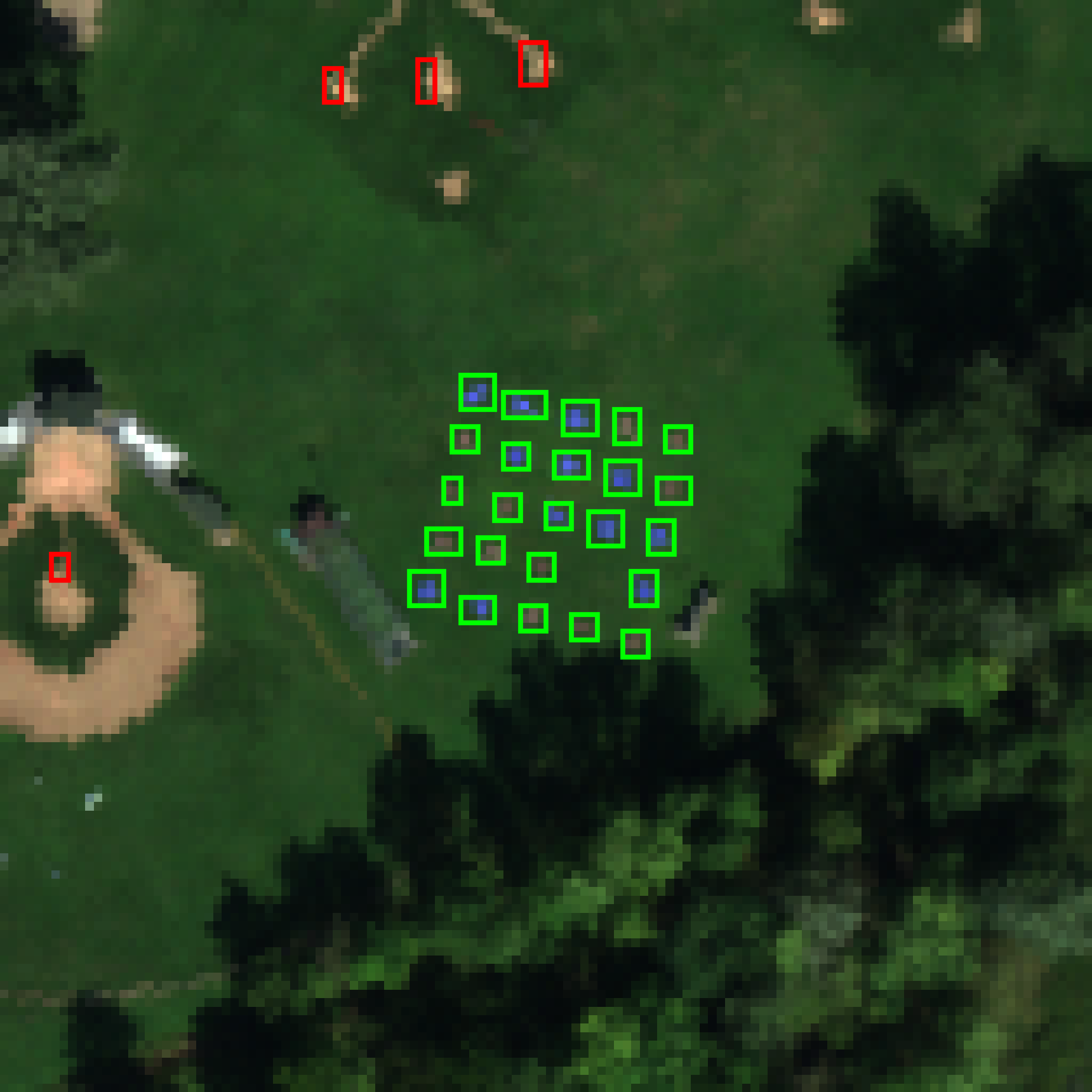
(a) SpecDETR

(b) ASD

(c) KASD

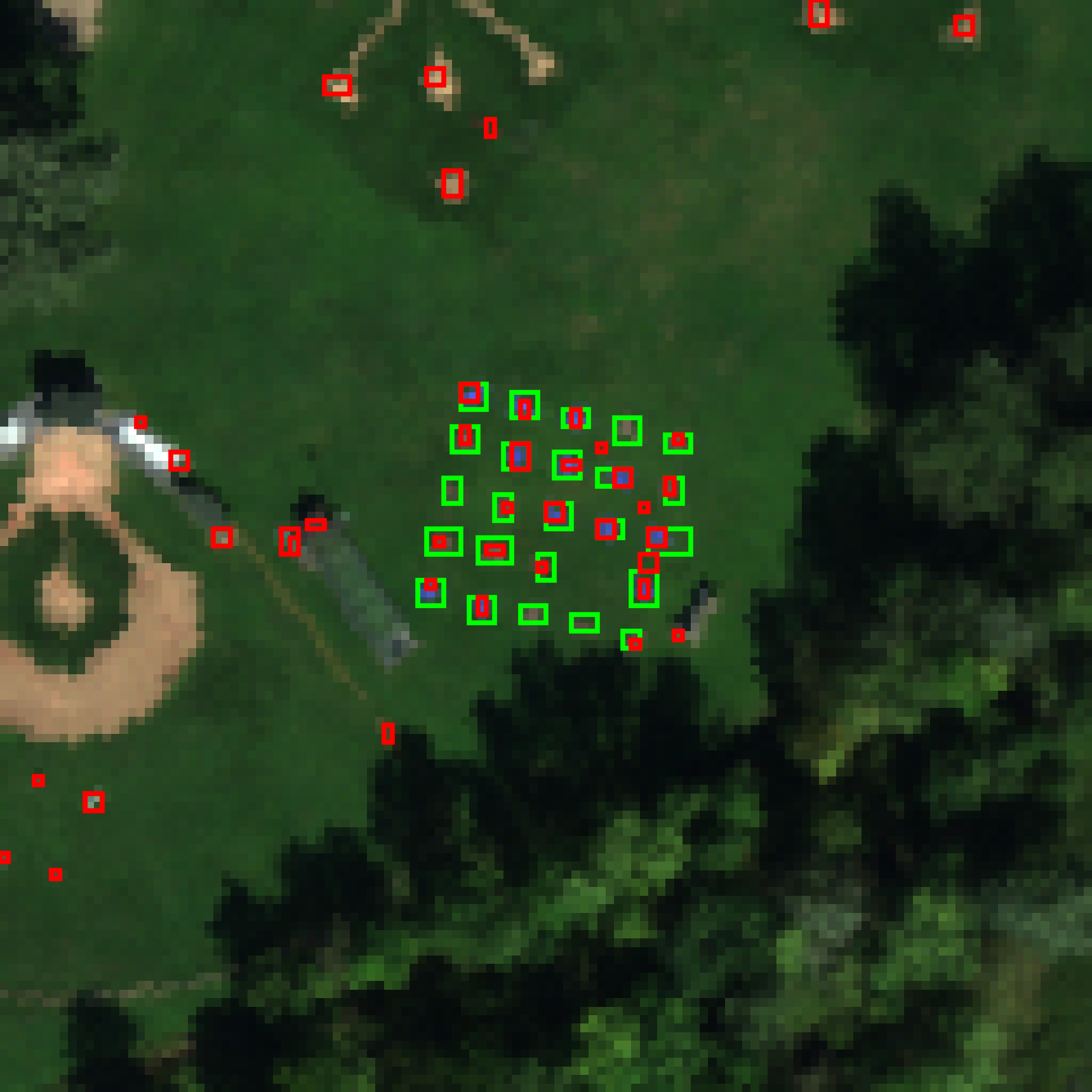
(d) CEM

(e) OSP

(f) TCIMF

Figure 13: Visualization results of SpecDETR and HTD methods on the Avon dataset. Green boxes are correct predictions, while red boxes are incorrect predictions.

TABLE VI: Comparison of the SpecDETR Decoder and DINO Decoder on the SPOD Dataset.

Decoder	mAP$\uparrow$			FLOPs$\downarrow$	Params$\downarrow$
	24epochs	36epochs	100epochs
DINO	0.663	0.759	0.849	143.6G	17.9M
SpecDETR	0.706($\uparrow$6.5%)	0.799($\uparrow$5.3%)	0.856	139.7G	16.1M($\downarrow$10.6%)

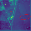
(a)

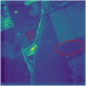
(b)

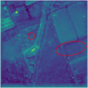
(c)

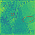
(d)

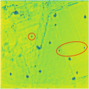
(e)

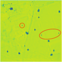
(f)

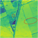
(a) The 1st layer

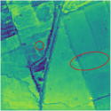
(b) The 2nd layer

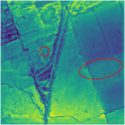
(c) The 3rd layer

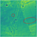
(d) The 4th layer

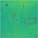
(e) The 5th layer

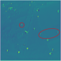
(f) The 6th layer

Figure 14: Feature maps generated by each encoder layer of SpecDETR on a test HSI from the SPOD dataset. The red circles highlight three subpixel objects.

DINO decoder is the SOTA DETR decoder among current DETR-like detectors, helping Co-DETR [72] achieve the best mAP of 0.66 on the COCO test-dev. By employing the SpecDETR encoder and LGC attention modules uniformly, we compare detectors with the DINO decoder and SpecDETR decoder in terms of point object detection accuracy, floating point operations (FLOPs), and the number of parameters on the SPOD dataset. As shown in Table VI, the SpecDETR decoder outperforms the DINO decoder in these metrics. Compared to the DINO decoder, the SpecDETR decoder achieves a 6.5% and 5.3% increase in mAP at 24 and 36 epochs settings, respectively. Meanwhile, the number of parameters is decreased by 10.6%.

V-D2 Positive and Negative Sample Setting

SpecDETR is a one-to-many set prediction problem, primarily reflected in the positive and negative sample setting, which includes the label assignment in the matching branch and the GT box noise addition in the denoising branch. As shown in Table VII, we investigate the impact of different positive and negative sample settings on the performance of SpecDETR. The label assignment considers one-to-one assignment (Forced Matching) and one-to-many assignment (Forced Matching + Dynamic Matching). For the denoising branch, we consider DN [44], CDN [19], our CCDN, and the case without denoising training. Under the three denoising ways, SpecDETR performs significantly better than the case without denoising training. This indicates that even when the matching part adopts one-to-many label assignment, SpecDETR still needs to rely on denoising training to accelerate convergence. Under one-to-many matching, CCDN outperforms CDN and DN. Additionally, under one-to-one label assignment, CDN is lower than DN by 2.2% and 1.7% in AP at 36 epochs and 100 epochs, respectively, because CDN generates negative samples that are highly similar to the GT, which interferes with the classification head of SpecDETR. Our one-to-many label assignment introduces more high-quality positive samples into the classification head from the matching branch. It improves detection performance regardless of whether DN, CDN, or CCDN is adopted.

V-D3 LGC Attention Module

Table VIII shows that with attention computation based only on local features, i.e., Eq. (3), SpecDETR achieves only 0.228 mAP, 0.54 mAP, and 0.804 mAP at 24 epochs, 36 epochs, and 100 epochs settings on the SPOD dataset, respectively. This indicates the necessity of introducing global spectral information into attention computation in SpecDETR. Compared to fixed sampling points, using deformable sampling points as described in equation Eq. (5) in SpecDETR results in improvements of 8.3%, 6.8%, and 2.0% in mAP at 24 epochs, 36 epochs, and 100 epochs, respectively.

V-D4 Content Query Initialization

As shown in Table IX, we explore the impact of different content query initialization for SpecDETR. “Constant” represents initializing all content queries as all one vectors, “Random” represents initializing queries with random values each time, and “Embedding” represents the index embedding in DINO [19]. SpecDETR converges fastest with the constant initialization. At 24 epochs, the constant initialization achieved an mAP that is 9.1% higher than the embedding initialization and 15.4% higher than the random initialization. DINO is regarded as a one-to-one set prediction problem, requiring embedding initialization for content queries to differentiate them. We consider SpecDETR as a one-to-many set prediction problem, so the initialization of content queries should be consistent.

TABLE VII: Performance Comparison of SpecDETR with Different Positive and Negative Sample Settings on the SPOD Dataset.

DeNosing	Lable Assigner		mAP
	Forced Matching	Dynamic Matching	36epochs	100epochs
✗	✓		0.611	0.796
	✓	✓	0.595	0.800
DN[44]	✓		0.773	0.836
	✓	✓	0.785	0.844
CDN[19]	✓		0.756	0.822
	✓	✓	0.791	0.846
CCDN	✓		0.780	0.829
	✓	✓	0.799	0.856

TABLE VIII: Performance Comparison of SpecDETR with Different Attention Modules on the SPOD Dataset.

Local	Global	Deformable	mAP
Attention	Attention	Sampling	24epochs	36epochs	100epochs
✓	✗	✓	0.228	0.540	0.804
✓	✓	✗	0.652	0.748	0.842
✓	✓	✓	0.706	0.799	0.856

V-D5 Redundant Predictions and NMS

In the classic evaluation on the COCO dataset [46], the top 100 prediction boxes are chosen, leading many detectors to provide numerous redundant predictions to boost mAP. However, in practical applications, a large number of redundant predictions are unnecessary. Therefore, in hyperspectral point object detection, SpecDETR places NMS as the last step to reduce redundant boxes in the final output predictions. As shown in Table X, we explore the impact of different IoU thresholds of NMS on the prediction count and detection performance of SpecDETR on the SPOD Dataset and Avon Dataset. On the SPOD Dataset, as the IoU threshold exceeds 0.5, both mAP and mAR improve. This is because previously misclassified predicted boxes now have corresponding redundant boxes with correct classes. When NMS is not used, mAP reaches 0.951. However, the increase in the IoU threshold also introduces redundant boxes. With the IoU threshold being set to the default value of 0.01, the output prediction count is only 10.4% of that without using NMS. For the Avon dataset, we round the predicted boxes, so there is no change in the prediction count with variations in the IoU threshold.

V-D6 Feature Extraction in SpecDETR Encoder

Fig. 14 visualizes the feature maps generated by different SpecDETR encoder layers. As the encoder layer number increases, the background area with the complex texture structure gradually smooths out, while objects gradually stand out from the background. We circle three subpixel objects with abundances below 0.2 in red. On the feature maps generated by the first encoder layer, these three objects are barely discernible, while on the feature maps generated by the last encoder layer, these three objects are very prominent. This indicates that our SpecDETR encoder can effectively extract useful information about objects from HSIs.

TABLE IX: AP Performance Comparison of SpecDETR with Different Content Query Initialization on the SPOD Dataset.

Content Query	24epochs	36epochs	100epochs
Embedding	0.647	0.771	0.845
Random	0.612	0.790	0.855
Constant	0.706	0.799	0.856

TABLE X: The Comparison of Prediction Count and Detection Performance of SpecDETR with different IoU Thresholds of NMS on the SPOD Dataset and Avon Dataset.

IoU Threshold	SPOD Dataset			Avon Dataset
	Predictions	mAP	mAR	Predictions	mAP	mAR
0.01	15615	0.856	0.897	28	0.885	0.925
0.1	15799	0.856	0.897	28	0.885	0.925
0.2	16101	0.856	0.897	28	0.885	0.925
0.3	16708	0.856	0.897	28	0.885	0.925
0.4	17844	0.856	0.897	28	0.885	0.925
0.5	20821	0.858	0.900	28	0.885	0.925
0.6	26334	0.860	0.904	28	0.885	0.925
0.7	31561	0.862	0.909	28	0.885	0.925
0.8	36095	0.864	0.915	28	0.885	0.925
0.9	41731	0.865	0.920	28	0.885	0.925
✗	150000	0.546	0.951	300	0.423	0.925

VI Supplementary Experiments in Infrared Small Target Detction

Infrared small target detection (IRSTD) aims to utilize grayscale and morphological abnormality information to search for interesting targets on single-channel infrared images. Consistent with traditional HTD methods, traditional IRSTD methods also employ a per-pixel binary classification framework, categorizing each pixel in the image as either background or target pixel. In recent years, deep learning-based IRSTD methods [48, 49, 73] have modeled IRSTD as a semantic segmentation problem, believing it helps to better address the performance degradation caused by small target areas. These segmentation networks are still considered the per-pixel binary classification framework but can learn general deep features of infrared small targets from a large number of training images, achieving detection performance superior to traditional IRSTD methods. In this section, we extend SpecDETR to the IRSTD task and evaluate SpecDETR and these segmentation networks’ object-level detection performance on three public IRSTD datasets.

TABLE XI: Image and Object Sample Information for Three Public IRSTD Datasets.

Dataset	IRSTD-1K [48]	IRSTD-1K	SIRST [73]	NUDT-SIRST [49]
		for SpecDETR
Training images	800	800	213	663
Test images	201	201	214	664
Training samples	1198	1188	270	918
Test samples	297	294	263	945
Image size	512$\times$512	256$\times$256	Max:592$\times$400	256$\times$256
			Min:135$\times$96
Sample size	Max:53$\times$56	Max:27$\times$28	Max:25$\times$24	Max:20$\times$14
	Min:1$\times$1	Min:1$\times$1	Min:2$\times$2	Min:1$\times$1

TABLE XII: Comparison of Detection Performance between SpecDETR and Seven IRSTD Networks on Three Public IRSTD Datasets.

Method	IRSTD-1K [48]						SIRST [73]						NUDT-SIRST [49]
	AP	$\text{AP}_{\text{25}}$	$\text{AP}_{\text{50}}$	AR	$\text{Re}_{\text{25}}$	$\text{Re}_{\text{50}}$	AP	$\text{AP}_{\text{25}}$	$\text{AP}_{\text{50}}$	AR	$\text{Re}_{\text{25}}$	$\text{Re}_{\text{50}}$	AP	$\text{AP}_{\text{25}}$	$\text{AP}_{\text{50}}$	AR	$\text{Re}_{\text{25}}$	$\text{Re}_{\text{50}}$
ACM [73]	0.286	0.795	0.664	0.465	0.919	0.822	0.340	0.905	0.760	0.484	0.924	0.833	0.398	0.942	0.870	0.547	0.965	0.921
ALCNet [74]	0.299	0.800	0.655	0.482	0.919	0.825	0.201	0.803	0.601	0.357	0.863	0.741	0.272	0.961	0.703	0.426	0.974	0.813
DNANet [49]	0.414	0.855	0.744	0.545	0.889	0.818	0.560	0.920	0.862	0.710	0.943	0.913	0.913	0.989	0.989	0.946	0.992	0.990
ISNet [48]	0.411	0.821	0.738	0.555	0.886	0.828	0.448	0.918	0.820	0.622	0.954	0.901	0.577	0.950	0.914	0.722	0.975	0.958
ISTDU-Net [75]	0.412	0.866	0.774	0.561	0.923	0.859	0.539	0.933	0.888	0.690	0.954	0.932	0.867	0.976	0.965	0.914	0.983	0.978
RDIAN [76]	0.377	0.802	0.720	0.523	0.869	0.808	0.468	0.903	0.815	0.629	0.935	0.882	0.599	0.976	0.927	0.731	0.982	0.956
UIUNet [77]	0.405	0.839	0.719	0.562	0.906	0.828	0.558	0.915	0.870	0.694	0.928	0.901	0.816	0.971	0.971	0.886	0.988	0.986
SpecDETR	0.415	0.841	0.740	0.574	0.929	0.850	0.541	0.930	0.894	0.666	0.943	0.913	0.812	0.955	0.946	0.876	0.984	0.980

VI-A Dataset

We select three public IRSTD datasets, namely IRSTD-1K [48], SIRST [73], and NUDT-SIRST [49]. These datasets consist of single-channel infrared images with per-pixel mask annotations, where all target pixels are considered as the same category. Following the previous practice [49] in the IRSTD field, we consider a connected set of target pixels in an eight-connected region as one object sample. We take the maximum bounding rectangle of the object as its box annotation and convert the mask annotations of the three datasets to box annotations. The statistical information of the images and target samples for the three datasets is shown in Table XI. Unlike the Avon and SPOD datasets in Section V, the object sizes in the three IRSTD datasets vary greatly. For example, the smallest object size in the NUDT-SIRST dataset is only 1x1 pixel, while the largest target size is 20x14 pixels. In addition, the image size of the IRSTD-1K dataset is 512x512. To avoid excessive VRAM usage of SpecDETR, we downsample the images in the IRSTD-1K dataset by 1/2. Some non-adjacent target pixels are connected by an eight-connectivity domain after the downsampling, resulting in a reduction of 10 training sample instances and 3 testing sample instances.

VI-B Implementation Details

Considering the lack of spectral information in single-channel infrared images, we remove the global token of SpecDETR’s attention module and increase the number of attention heads from 8 to 16, providing more sampling points to better perceive local shape information. As the image sizes of the three IRSTD datasets are relatively large, we reduce the number of encoder and decoder layers of SpecDETR from 6 to 3. Additionally, we round the predicted boxes and filter out those with confidence scores less than 0.1. The other parameters of SpecDETR were set the same as in Section V.

We select seven segmentation-based IRSTD networks, ACM [73], ALCNet [74], DNANet [49], ISNet [48], ISTDU-Net [75], RDIAN [76], and UIUNet [77], as the comparison methods, and obtain their detection results from the BasicIRSTD toolbox. To estimate the object-level detection performance, we convert the per-pixel prediction results of the seven comparison methods into object-level box prediction results. Similar to the mask annotation conversion, we regard a connected set of predicted target pixels in an eight-connectivity domain as a predicted object, and take the maximum bounding box enclosing the target pixels as the predicted box, with the maximum confidence score of the target pixels as the predicted score.

We compare the AP, AR, and APs and recalls at IoU thresholds of 0.25 and 0.5 between SpecDETR and the seven IRSTD networks.

VI-C Result Analysis

As shown in Table XII, our SpecDETR achieves comparable object-level detection performance to the current SOTA IRSTD networks on the IRSTD-1K and SIRST datasets. Particularly on the IRSTD-1K dataset, SpecDETR achieves a best AP of 0.415 and a best AR of 0.574, despite using smaller image sizes (256x265 instead of 512x512) and coarser bounding box annotations instead of per-pixel masks. On the NUDT-SIRST dataset, SpecDETR achieves an AP of 0.812 and an AR of 0.876, while DNANet outperforms other IRSTD networks and SpecDETR significantly. After excluding DNANet, SpecDETR performs comparably to the remaining IRSTD networks such as UIUNet and ISTDU-Net.

Although SpecDETR is designed for point object detection, the experiments on the three IRSTD datasets demonstrate that SpecDETR still possesses the detection capability for larger and shaped objects. Despite being trained with coarse box annotations, while IRSTD networks are trained with fine-grained per-pixel mask annotations, SpecDETR does not show inferiority to IRSTD networks in object-level detection evaluation. The question of whether the IRSTD task must adhere to the per-pixel binary classification framework, which needs laborious and time-consuming per-pixel mask annotations, is worth further discussion.

VII Conclusion

In this paper, we extended the hyperspectral point target detection task to the hyperspectral point object detection task, highlighting the crucial role of spectral information in point object detection. Through experiments on a synthetic and public dataset, we demonstrated the significant superiority of our proposed SpecDETR in point object detection. However, due to limitations in the current development of the field, we have yet to validate the capability of SpecDETR to detect composite-spectra point objects in the real world. In the future, we will develop a large-scale, real-world hyperspectral point object detection dataset to advance this task further.

References

- [1] C. Zhao, B. Qin, S. Feng, W. Zhu, W. Sun, W. Li, and X. Jia, “Hyperspectral image classification with multi-attention transformer and adaptive superpixel segmentation-based active learning,” IEEE Trans. Image Process., 2023.
- [2] L. Drumetz, J. Chanussot, C. Jutten, W.-K. Ma, and A. Iwasaki, “Spectral variability aware blind hyperspectral image unmixing based on convex geometry,” IEEE Trans. Image Process., vol. 29, pp. 4568–4582, 2020.
- [3] J. E. Fowler and Q. Du, “Anomaly detection and reconstruction from random projections,” IEEE Trans. Image Process., vol. 21, no. 1, pp. 184–195, 2011.
- [4] Z. Li, Y. Wang, C. Xiao, Q. Ling, Z. Lin, and W. An, “You only train once: Learning a general anomaly enhancement network with random masks for hyperspectral anomaly detection,” IEEE Trans. Geosci. Remote Sens., vol. 61, pp. 1–18, 2023.
- [5] B. Du, Y. Zhang, L. Zhang, and D. Tao, “Beyond the sparsity-based target detector: A hybrid sparsity and statistics-based detector for hyperspectral images,” IEEE Trans. Image Process., vol. 25, no. 11, pp. 5345–5357, 2016.
- [6] Y. Li, Y. Shi, K. Wang, B. Xi, J. Li, and P. Gamba, “Target detection with unconstrained linear mixture model and hierarchical denoising autoencoder in hyperspectral imagery,” IEEE Trans. Image Process., vol. 31, pp. 1418–1432, 2022.
- [7] G. Xia, X. Bai, J. Ding, Z. Zhu, S. Belongie, J. Luo, M. Datcu, M. Pelillo, and L. Zhang, “DOTA: A large-scale dataset for object detection in aerial images,” in IEEE Conf. Comput. Vis. Pattern Recog., 2018, pp. 3974–3983.
- [8] G. Vane, R. O. Green, T. G. Chrien, H. T. Enmark, E. G. Hansen, and W. M. Porter, “The airborne visible/infrared imaging spectrometer (AVIRIS),” Remote sensing of environment, vol. 44, no. 2-3, pp. 127–143, 1993.
- [9] C. E. Caefer, S. R. Rotman, J. Silverman, and P. W. Yip, “Algorithms for point target detection in hyperspectral imagery,” in Imaging Spectrometry VIII, vol. 4816. SPIE, 2002, pp. 242–257.
- [10] J. C. Harsanyi, “Detection and classification of subpixel spectral signatures in hyperspectral image sequences,” Ph.D. dissertation, University of Maryland Baltimore County, Baltimore, MD, USA, 1993.
- [11] H. Ren and C.-I. Chang, “Target-constrained interference-minimized approach to subpixel target detection for hyperspectral images,” Opt. Eng., vol. 39, pp. 3138–3145, 2000.
- [12] T. Wang, B. Du, and L. Zhang, “A kernel-based target-constrained interference-minimized filter for hyperspectral sub-pixel target detection,” IEEE J. Sel. Topics Appl. Earth Observ. Remote Sens., vol. 6, no. 2, pp. 626–637, Apr. 2013.
- [13] S. Ren, K. He, R. Girshick, and J. Sun, “Faster R-CNN: Towards real-time object detection with region proposal networks,” in Adv. Neural Inform. Process. Syst., vol. 28, 2015.
- [14] J. Redmon, S. Divvala, R. Girshick, and A. Farhadi, “You only look once: Unified, real-time object detection,” in IEEE Conf. Comput. Vis. Pattern Recog., 2016, pp. 779–788.
- [15] N. Carion, F. Massa, G. Synnaeve, N. Usunier, A. Kirillov, and S. Zagoruyko, “End-to-end object detection with transformers,” in Eur. Conf. Comput. Vis., 2020, pp. 213–229.
- [16] S. Kumar, I. Arevalo, A. Iftekhar, and B. Manjunath, “Methanemapper: Spectral absorption aware hyperspectral transformer for methane detection,” in IEEE Conf. Comput. Vis. Pattern Recog., 2023, pp. 17 609–17 618.
- [17] A. Vaswani, N. Shazeer, N. Parmar, J. Uszkoreit, L. Jones, A. N. Gomez, Ł. Kaiser, and I. Polosukhin, “Attention is all you need,” Adv. Neural Inform. Process. Syst., vol. 30, 2017.
- [18] X. Zhu, W. Su, L. Lu, B. Li, X. Wang, and J. Dai, “Deformable DETR: Deformable transformers for end-to-end object detection,” arXiv, 2020.
- [19] H. Zhang, F. Li, S. Liu, L. Zhang, H. Su, J. Zhu, L. M. Ni, and H.-Y. Shum, “DINO: DETR with improved denoising anchor boxes for end-to-end object detection,” arXiv, 2022.
- [20] N. M. Nasrabadi, “Hyperspectral target detection : An overview of current and future challenges,” IEEE Signal Process. Mag., vol. 31, no. 1, pp. 34–44, Dec. 2013.
- [21] F. C. Robey, D. R. Fuhrmann, E. J. Kelly, and R. Nitzberg, “A CFAR adaptive matched filter detector,” IEEE Trans. Aerosp. Electron. Syst., vol. 28, no. 1, pp. 208–216, Jan. 1992.
- [22] S. Kraut, L. L. Scharf, and R. W. Butler, “The adaptive coherence estimator: A uniformly most-powerful-invariant adaptive detection statistic,” IEEE Trans. Signal Process., vol. 53, no. 2, pp. 427–438, Feb 2005.
- [23] B. Du, Y. Zhang, L. Zhang, and D. Tao, “Beyond the sparsity-based target detector: A hybrid sparsity and statistics based detector for hyperspectral images,” IEEE Trans. Image Process., vol. 25, no. 11, pp. 5345–5357, Nov. 2016.
- [24] S. Kraut and L. L. Scharf, “The CFAR adaptive subspace detector is a scale-invariant GLRT,” IEEE Trans. Signal Process., vol. 47, no. 9, pp. 2538–2541, Sep. 1999.
- [25] J. C. Harsanyi and C.-I. Chang, “Hyperspectral image classification and dimensionality reduction: An orthogonal subspace projection approach,” IEEE Trans. Geosci. Remote Sens., vol. 32, no. 4, pp. 779–785, Jul. 1994.
- [26] Y. Chen, N. M. Nasrabadi, and T. D. Tran, “Simultaneous joint sparsity model for target detection in hyperspectral imagery,” IEEE Geosci. Remote Sens. Lett., vol. 8, no. 4, pp. 676–680, Jul. 2011.
- [27] Y. Chen, N. M. Nasrabadi, and T. D. Tran, “Sparse representation for target detection in hyperspectral imagery,” IEEE J. Sel. Topics Signal Process., vol. 5, no. 3, pp. 629–640, Jun. 2011.
- [28] Y. Chen, N. M. Nasrabadi, and T. D. Tran, “Hyperspectral image classification via kernel sparse representation,” IEEE Trans. Geosci. Remote Sens., vol. 51, no. 1, pp. 217–231, Jan. 2013.
- [29] Y. Zhang, B. Du, and L. Zhang, “A sparse representation-based binary hypothesis model for target detection in hyperspectral images,” IEEE Trans. Geosci. Remote Sens., vol. 53, no. 3, pp. 1346–1354, Mar. 2015.
- [30] Q. Ling, Y. Guo, Z. Lin, L. Liu, and W. An, “A constrained sparse-representation-based binary hypothesis model for target detection in hyperspectral imagery,” IEEE J. Sel. Topics Appl. Earth Observ. Remote Sens., vol. 12, no. 6, pp. 1933–1947, 2019.
- [31] Y. Zhang, L. Zhang, B. Du, and S. Wang, “A nonlinear sparse representation-based binary hypothesis model for hyperspectral target detection,” IEEE J. Sel. Topics Appl. Earth Observ. Remote Sens., vol. 8, no. 6, pp. 2513–2522, Jun. 2015.
- [32] X. Jiao and C.-I. Chang, “Kernel-based constrained energy minimization (K-CEM),” in Algorithms and Technologies for Multispectral, Hyperspectral, and Ultraspectral Imagery XIV. SPIE, 2008, pp. 523–533.
- [33] H. Kwon and N. M. Nasrabadi, “Kernel orthogonal subspace projection for hyperspectral signal classification,” IEEE Trans. Geosci. Remote Sens., vol. 43, no. 12, pp. 2952–2962, 2005.
- [34] H. Kwon and N. M. Nasrabadi, “A comparative analysis of kernel subspace target detectors for hyperspectral imagery,” EURASIP Journal on Advances in Signal Processing, vol. 2007, pp. 1–13, 2006.
- [35] H. Kwon and N. M. Nasrabadi, “Kernel matched subspace detectors for hyperspectral target detection,” IEEE Trans. Pattern Anal. Mach. Intell., vol. 28, no. 2, pp. 178–194, Feb 2006.
- [36] G. Camps-Valls, L. Gomez-Chova, J. Munoz-Marí, J. Vila-Francés, and J. Calpe-Maravilla, “Composite kernels for hyperspectral image classification,” IEEE Geosci. Remote Sens. Lett., vol. 3, no. 1, pp. 93–97, Jan. 2006.
- [37] W. Rao, L. Gao, Y. Qu, X. Sun, B. Zhang, and J. Chanussot, “Siamese transformer network for hyperspectral image target detection,” IEEE Trans. Geosci. Remote Sens., vol. 60, pp. 1–19, 2022.
- [38] D. Zhu, B. Du, and L. Zhang, “Two-stream convolutional networks for hyperspectral target detection,” IEEE Trans. Geosci. Remote Sens., vol. 59, no. 8, pp. 6907–6921, 2020.
- [39] L. Yan, M. Zhao, X. Wang, Y. Zhang, and J. Chen, “Object detection in hyperspectral images,” IEEE Signal Process. Lett., vol. 28, pp. 508–512, 2021.
- [40] G. Lee, J. Lee, J. Baek, H. Kim, and D. Cho, “Channel sampler in hyperspectral images for vehicle detection,” IEEE Geosci. Remote Sens. Lett., vol. 19, pp. 1–5, 2021.
- [41] A. Rangnekar, Z. Mulhollan, A. Vodacek et al., “Semi-supervised hyperspectral object detection challenge results-PBVS 2022,” in IEEE Conf. Comput. Vis. Pattern Recog. Worksh., 2022, pp. 390–398.
- [42] X. He, C. Tang, X. Liu, W. Zhang, K. Sun, and J. Xu, “Object detection in hyperspectral image via unified spectral–spatial feature aggregation,” IEEE Trans. Geosci. Remote Sens., vol. 61, pp. 1–13, 2023.
- [43] S. Liu, F. Li, H. Zhang, X. Yang, X. Qi, H. Su, J. Zhu, and L. Zhang, “DAD-DETR: Dynamic anchor boxes are better queries for DETR,” arXiv, 2022.
- [44] F. Li, H. Zhang, S. Liu, J. Guo, L. M. Ni, and L. Zhang, “DN-DETR: Accelerate DETR training by introducing query denoising,” in IEEE Conf. Comput. Vis. Pattern Recog., 2022, pp. 13 619–13 627.
- [45] Q. Chen, X. Chen, J. Wang, S. Zhang, K. Yao, H. Feng, J. Han, E. Ding, G. Zeng, and J. Wang, “Group DETR: Fast DETR training with group-wise one-to-many assignment,” in Int. Conf. Comput. Vis., 2023, pp. 6633–6642.
- [46] T.-Y. Lin, M. Maire, S. Belongie, J. Hays, P. Perona, D. Ramanan, P. Dollár, and C. L. Zitnick, “Microsoft COCO: Common objects in context,” in Eur. Conf. Comput. Vis., 2014, pp. 740–755.
- [47] G. Cheng, X. Yuan, X. Yao, K. Yan, Q. Zeng, X. Xie, and J. Han, “Towards large-scale small object detection: Survey and benchmarks,” IEEE Trans. Pattern Anal. Mach. Intell., 2023.
- [48] M. Zhang, R. Zhang, Y. Yang, H. Bai, J. Zhang, and J. Guo, “Isnet: Shape matters for infrared small target detection,” in IEEE Conf. Comput. Vis. Pattern Recog., 2022, pp. 877–886.
- [49] B. Li, C. Xiao, L. Wang, Y. Wang, Z. Lin, M. Li, W. An, and Y. Guo, “Dense nested attention network for infrared small target detection,” IEEE Trans. Image Process., vol. 32, pp. 1745–1758, 2022.
- [50] J. L. Ba, J. R. Kiros, and G. E. Hinton, “Layer normalization,” arXiv, 2016.
- [51] A. Giannandrea, N. Raqueno, D. W. Messinger, J. Faulring, J. P. Kerekes et al., “The share 2012 data campaign,” in Algorithms and Technologies for Multispectral, Hyperspectral, and Ultraspectral Imagery XIX. SPIE, 2013, pp. 94–108.
- [52] J. Dai, H. Qi, Y. Xiong, Y. Li, G. Zhang, H. Hu, and Y. Wei, “Deformable convolutional networks,” in Int. Conf. Comput. Vis., 2017, pp. 764–773.
- [53] J. Liu and J. Zhang, “Spectral unmixing via compressive sensing,” IEEE Trans. Geosci. Remote Sens., vol. 52, no. 11, pp. 7099–7110, Nov. 2014.
- [54] R. Kokaly, R. Clark, G. Swayze, K. Livo, T. Hoefen, N. Pearson, R. Wise, W. Benzel, H. Lowers, R. Driscoll et al., “USGS spectral library version 7 data: US geological survey data release,” United States Geological Survey (USGS): Reston, VA, USA, vol. 61, 2017.
- [55] K. Chen, J. Wang, J. Pang, Y. Cao et al., “MMDetection: Open mmlab detection toolbox and benchmark,” arXiv, 2019.
- [56] L. L. Scharf and B. Friedlander, “Matched subspace detectors,” IEEE Trans. Signal Process., vol. 42, no. 8, pp. 2146–2157, Aug. 1994.
- [57] C.-I. Chang, “An effective evaluation tool for hyperspectral target detection: 3D receiver operating characteristic curve analysis,” IEEE Trans. Geosci. Remote Sens., vol. 59, no. 6, pp. 5131–5153, 2020.
- [58] K. He, X. Zhang, S. Ren, and J. Sun, “Deep residual learning for image recognition,” in IEEE Conf. Comput. Vis. Pattern Recog., 2016, pp. 770–778.
- [59] I. Radosavovic, R. P. Kosaraju, R. Girshick, K. He, and P. Dollár, “Designing network design spaces,” in IEEE Conf. Comput. Vis. Pattern Recog., 2020, pp. 10 428–10 436.
- [60] H. Zhang, C. Wu, Z. Zhang, Y. Zhu, H. Lin, Z. Zhang, Y. Sun, T. He, J. Mueller, R. Manmatha et al., “ResNeSt: Split-attention networks,” in IEEE Conf. Comput. Vis. Pattern Recog., 2022, pp. 2736–2746.
- [61] S. Xie, R. Girshick, P. Dollár, Z. Tu, and K. He, “Aggregated residual transformations for deep neural networks,” in IEEE Conf. Comput. Vis. Pattern Recog., 2017, pp. 1492–1500.
- [62] K. Sun, B. Xiao, D. Liu, and J. Wang, “Deep high-resolution representation learning for human pose estimation,” in IEEE Conf. Comput. Vis. Pattern Recog., 2019, pp. 5693–5703.
- [63] C. Feng, Y. Zhong, Y. Gao, M. R. Scott, and W. Huang, “TOOD: Task-aligned one-stage object detection,” in Int. Conf. Comput. Vis., 2021, pp. 3490–3499.
- [64] Z. Dong, G. Li, Y. Liao, F. Wang, P. Ren, and C. Qian, “Centripetalnet: Pursuing high-quality keypoint pairs for object detection,” in IEEE Conf. Comput. Vis. Pattern Recog., 2020, pp. 10 519–10 528.
- [65] A. Newell, K. Yang, and J. Deng, “Stacked hourglass networks for human pose estimation,” in Eur. Conf. Comput. Vis. Springer, 2016, pp. 483–499.
- [66] H. Law and J. Deng, “Cornernet: Detecting objects as paired keypoints,” in Eur. Conf. Comput. Vis., 2018, pp. 734–750.
- [67] Z. Yang, S. Liu, H. Hu, L. Wang, and S. Lin, “Reppoints: Point set representation for object detection,” in IEEE Conf. Comput. Vis. Pattern Recog., 2019, pp. 9657–9666.
- [68] T.-Y. Lin, P. Goyal, R. Girshick, K. He, and P. Dollár, “Focal loss for dense object detection,” in IEEE Conf. Comput. Vis. Pattern Recog., 2017, pp. 2980–2988.
- [69] M. Tan and Q. Le, “Efficientnet: Rethinking model scaling for convolutional neural networks,” in ICML, 2019, pp. 6105–6114.
- [70] W. Wang, E. Xie, X. Li, D.-P. Fan, K. Song, D. Liang, T. Lu, P. Luo, and L. Shao, “PVTv2: Improved baselines with pyramid vision transformer,” Computational Visual Media, vol. 8, no. 3, pp. 415–424, 2022.
- [71] Z. Liu, Y. Lin, Y. Cao, H. Hu, Y. Wei, Z. Zhang, S. Lin, and B. Guo, “Swin Transformer: Hierarchical vision transformer using shifted windows,” in Int. Conf. Comput. Vis., 2021, pp. 10 012–10 022.
- [72] Z. Zong, G. Song, and Y. Liu, “Detrs with collaborative hybrid assignments training,” in Int. Conf. Comput. Vis., 2023, pp. 6748–6758.
- [73] Y. Dai, Y. Wu, F. Zhou, and K. Barnard, “Asymmetric contextual modulation for infrared small target detection,” in IEEE Winter Conference on Applications of Computer Vision, 2021, pp. 950–959.
- [74] Y. Dai, Y. Wu, F. Zhou, and K. Barnard, “Attentional local contrast networks for infrared small target detection,” IEEE Trans. Geosci. Remote Sens., vol. 59, no. 11, pp. 9813–9824, 2021.
- [75] Q. Hou, L. Zhang, F. Tan, Y. Xi, H. Zheng, and N. Li, “ISTDU-Net: Infrared small-target detection U-Net,” IEEE Geosci. Remote Sens. Lett., vol. 19, pp. 1–5, 2022.
- [76] H. Sun, J. Bai, F. Yang, and X. Bai, “Receptive-field and direction induced attention network for infrared dim small target detection with a large-scale dataset irdst,” IEEE Trans. Geosci. Remote Sens., vol. 61, pp. 1–13, 2023.
- [77] X. Wu, D. Hong, and J. Chanussot, “UIU-Net: U-Net in U-Net for infrared small object detection,” IEEE Trans. Image Process., vol. 32, pp. 364–376, 2022.