Single-ensemble multilevel Monte Carlo for discrete interacting-particle methods

Abstract

To solve problems in domains such as filtering, optimization, and posterior sampling, interacting-particle methods have recently received much attention. These parallelizable and often gradient-free algorithms use an ensemble of particles that evolve in time, based on a combination of well-chosen dynamics and interaction between the particles. For computationally expensive dynamics – for example, dynamics that solve inverse problems with an expensive forward model – the cost of attaining a high accuracy quickly becomes prohibitive. We exploit a hierarchy of approximations to this forward model and apply multilevel Monte Carlo (MLMC) techniques, improving the asymptotic cost-to-error relation. More specifically, we use MLMC at each time step to estimate the interaction term within a single, globally-coupled ensemble. This technique was proposed by Hoel et al. in the context of the ensemble Kalman filter; the goal of the present paper is to study its applicability to a general framework of interacting-particle methods. After extending the algorithm and its analysis to a broad set of methods with fixed numbers of time steps, we motivate the application of the method to the class of algorithms with an infinite time horizon, which includes popular methods such as ensemble Kalman algorithms for optimization and sampling. Numerical tests confirm the improved asymptotic scaling of the multilevel approach.

65C05, 65C35, 65Y20, 62F15

1 Introduction

This paper studies interacting-particle methods (IPMs), algorithms that solve various problems with an ensemble (or collection) of particles (or points, evolving over time in, e.g., a state or parameter space). Three problem classes for which IPMs have been particularly successful are filtering [1, 2, 3, 10, 15], optimization [28, 34, 38], and Bayesian-posterior sampling [5, 17, 27]. Simulated with a finite ensemble size $J$, IPMs can be viewed as Monte Carlo approximations to a corresponding mean-field model. Some example methods are introduced in Section 1.1.

Our main contribution is comparing this straightforward approximation to a newly proposed multilevel Monte Carlo (MLMC) scheme. MLMC is discussed in Section 1.2, after which we can state our goal and discuss related literature in Section 1.3. Section 1.4 summarizes the layout of the paper.

1.1 Interacting-particle methods

This subsection discusses the use of IPMs for filtering, optimization in Bayesian inverse problems, and posterior sampling. The first of these domains, filtering, is concerned with reconstructing state variables from noisy observations. Consider the discrete dynamics

(1) $$u_{n+1}=\mathcal{G}_{n}(u_{n}),\qquad 0\leq n<N,$$

where $u_{n}\in\mathbb{R}^{d_{u}}$ denotes the state at time step $n$ and $\mathcal{G}_{n}$ is the potentially stochastic forward model at that same time step. Now assume access to noisy observations

(2) $$y_{n}=Hu_{n}+\eta_{n},\qquad 0<n\leq N,$$

with $H$ a linear state-to-observation map and $\eta_{n}$ a noise term. The filtering problem is to estimate the states $\{u_{n}\}_{n=1}^{N}$ based on these noisy observations. One popular filtering algorithm is the ensemble Kalman filter (EnKF).

Example 1.1 (Ensemble Kalman filter).

The EnKF [15] is an IPM whose $J$ particles $\{u_{n}^{j}\}_{j=1}^{J}$ at time $n$ estimate the expectation and uncertainty on $u_{n}$. It assumes that $\eta_{n}\sim\mathcal{N}(0,\Gamma)$ for some positive definite $\Gamma$. An ensemble member $u_{n}^{j}$ evolves as

(3) $$u_{n+1}^{j}=(I-K_{n}H)\mathcal{G}_{n}(u_{n}^{j})+K_{n}(y_{n+1}+\sqrt{\Gamma}\eta_{n}^{j}),$$

where $K_{n}=C_{n}^{gg}H^{\mathstrut\scriptscriptstyle{\top}}(HC_{n}^{gg}H^{\mathstrut\scriptscriptstyle{\top}}+\Gamma)^{-1}$ (with $C_{n}^{gg}$ the sample covariance of $\{\mathcal{G}_{n}(u_{n}^{j})\}_{j}$) is called the Kalman gain, and where $\eta_{n}^{j}\sim\mathcal{N}(0,I)$. Theoretical studies of the EnKF and its properties often consider its mean-field limit (the limit for an infinite number of particles); convergence to that limit for finite $J$ is quantified in [31, 32].

A second problem class is that of Bayesian inverse problems. Here, we assume to have a single, deterministic forward map $\mathcal{G}\colon\mathbb{R}^{d_{u}}\rightarrow\mathbb{R}^{d_{g}}$ and an unknown parameter $u\in\mathbb{R}^{d_{u}}$. We are given a prior distribution $\pi_{\mathrm{prior}}(u)$ on $u$ and an observation

(4) $$y=\mathcal{G}(u)+\eta,$$

in which $\eta\in\mathbb{R}^{d_{g}}$ follows a known noise model $\pi_{\eta}$, such that we can define the likelihood $\pi_{\mathrm{li}}(y\mid u)\coloneqq\pi_{\eta}(y-\mathcal{G}(u))$. Bayes’ formula results in the posterior distribution

(5) $$\pi_{\mathrm{post}}(u\mid y)=\frac{\pi_{\mathrm{li}}(y\mid u)\pi_{\mathrm{prior}}(u)}{\pi_{\mathrm{ev}}(y)}.$$

The evidence $\pi_{\mathrm{ev}}(y)$ in Eq. 5 is usually intractable to compute, as it involves integration over the entire parameter domain. Hence, we work under the assumption that only an unnormalized posterior $\pi_{\mathrm{post}}(u\mid y)\propto\pi_{\mathrm{li}}(y\mid u)\pi_{\mathrm{prior}}(u)$ is available.

The posterior distribution is used in two main ways. Optimization methods can target the maximum a posteriori (MAP) parameter, the most likely $u$ value given $y$ and $\pi_{\mathrm{prior}}$. A more complete view of the posterior and its features is provided by sampling methods, which construct a sequence of $u$ values distributed according to $\pi_{\mathrm{post}}(u\mid y)$. IPMs that perform these tasks include ensemble Kalman inversion (EKI) [28] and ensemble Kalman sampling (EKS) [17], both inspired by the EnKF.

Example 1.2 (Ensemble Kalman inversion).

We again assume that $\eta\sim\mathcal{N}(0,\Gamma)$ and now require a uniform prior on $u$. (General noise distributions are handled in [13]; prior regularization is discussed in, e.g., [8, 26].) EKI was proposed as the iterated application of the EnKF (creating an artificial discrete time dimension) in [28], to which time steps $\tau_{n}$ were added in [38]. With $\eta_{n}^{j}\sim\mathcal{N}(0,I)$, the resulting dynamics are

(6) $$u_{n+1}^{j}=u_{n}^{j}+\tau_{n}C^{ug}_{n}(\tau_{n}C^{gg}_{n}+\Gamma)^{-1}(y-\mathcal{G}(u_{n}^{j})+\sqrt{\Gamma/\tau_{n}}\kern 2.0pt\eta_{n}^{j}),\qquad 1\leq j\leq J,$$

where $C_{n}^{ug}$ is the sample covariance of $\{u_{n}^{j}\}_{j}$ and $\{\mathcal{G}(u_{n}^{j})\}_{j}$. A continuous-time limit was studied in [38] and re-discretized in a slightly different form in, e.g., [30] – in that work, the (artificial) time steps $\tau_{n}$ are also determined adaptively adaptively. For simplicity, we omit this adaptivity and fix all $\tau_{n}$ in advance. Increasing $J$ improves exploration capabilities and reveals connections to gradient descent [4].

Example 1.3 (Ensemble Kalman sampling).

Assume again that $\eta\sim\mathcal{N}(0,\Gamma)$ and consider $\pi_{\mathrm{prior}}(u)$ a zero-centered Gaussian with covariance $\Gamma_{0}$. EKS was proposed and motivated in continuous-time form in [17]. In practice, a discretization should be used instead, and a common one is the linearly implicit split-step scheme (see [17])

(7a) $$u_{n+1}^{*,j} =u_{n}^{j}+\tau_{n}C_{n}^{ug}\Gamma^{-1}(y-\mathcal{G}(u_{n}^{j}))-\tau_{n}C_{n}^{uu}\Gamma_{0}^{-1}u_{n+1}^{*,j},$$

(7b) $$u_{n+1}^{j} =u_{n+1}^{*,j}+\sqrt{2\tau_{n}C_{n}^{uu}}\kern 2.0pt\eta_{n}^{j},$$

where $C_{n}^{uu}$ is the sample covariance of $\{u_{n}^{j}\}_{j}$ and where $\eta_{n}^{j}\sim\mathcal{N}(0,I)$. These dynamics estimate the posterior Eq. 5, based on linear and Gaussian ansatzes, as $n\rightarrow\infty$. Like many ensemble Kalman methods, EKS is motivated by its mean-field limit [17], and a larger $J$ implies better performance [17] and convergence to the mean-field limit [12].

Two classes of IPMs

While the above division in terms of problem classes is natural from an application point of view, the example IPMs reveal another distinction, relevant to algorithm development and analysis throughout the paper. We distinguish two classes of discrete-time IPMs based on their time dimension:

• IPMs with a fixed number of discrete time steps. The ensemble Kalman filter falls into this category, as do other filtering algorithms such as the deterministic ensemble Kalman filter (DEnKF) [37].

• IPMs with an infinite number of discrete time steps. The EKS and EKI algorithms use discrete time-stepping, but their target is the particle distribution for the time step $n\rightarrow\infty$. Another example in this class are the consensus-based sampling (CBS) algorithm and its variants [5].

While many of the IPMs in this paper discretize continuous-time equations, refinement to obtain lower errors typically uses more particles over more time steps, while keeping the time step length (e.g., [6, 17, 34]). This justifies classifying them as discrete-time methods. Other IPMs, such as the ensemble Kalman–Bucy filter [2] or EKI’s sampling variant (see [11]), are defined in continuous time over a fixed interval – lowering their error involves refinement in time. Those IPMs are outside the scope of this paper.

Advantages of IPMs

Many of these methods require no derivatives of the forward model; instead of gradient information, interaction between the ensemble members drives the particle evolution. This is crucial when gradients are expensive, unavailable, or undefined due to a non-differentiable objective [30], or when they are noisy or highly oscillatory [14]. In addition, these methods allow for straightforward parallelization, as only the interaction term requires information from multiple particles.

Error sources for finite ensembles

When simulating an IPM with a finite number of particles $J$, the interaction term depends on the stochastic positions of all particles. Hence, simulating IPMs with a finite $J$ should be interpreted as an approximation to a theoretical mean-field model. In fact, when the end goal of IPM simulation is the final particle distribution, three sources of errors compound:

1. The interaction effect at each time is computed based on a finite number of particles. This introduces a bias and a statistical error in the dynamics.

2. The finite ensemble size introduces a statistical error on the final distribution.

3. A bias on the final particle distribution is introduced in infinite-time IPMs, as we must truncate the time dimension in practical simulations.

It is plausible that error sources 1 and 2 decrease when the number of particles $J$ increases. For many methods, it turns out that this happens at the $\mathcal{O}(J^{-1/2})$ rate typical for Monte Carlo [11, 12]. When particle evolution is computationally expensive due to a complex forward model in the underlying problem, attaining a high accuracy through straightforward Monte Carlo simulation of the IPM can become prohibitive.

1.2 Multilevel Monte Carlo

To simulate interacting-particle methods with expensive forward models more quickly, this paper will use multilevel Monte Carlo (MLMC) [18]. The core MLMC idea is as follows. An expectation $\mathbb{E}[X^{L}]$ of a computationally expensive random variable $X^{L}$, to which a hierarchy of cheaper and less accurate approximations $\{X^{\ell}\}_{\ell=0}^{L-1}$ is available, is rewritten with a telescoping sum:

(8) $$\mathbb{E}[X^{L}]=\mathbb{E}[X^{0}]+\sum\nolimits_{\ell=1}^{L}\mathbb{E}[X^{\ell}-X^{\ell-1}].$$

MLMC uses this representation to approximate $\mathbb{E}[X^{L}]$. Many cheap realizations of $X^{0}$ are sampled, giving an accurate estimate of $\mathbb{E}[X^{0}]$. The difference terms are then each approximated by sampling correlated realizations of $X^{\ell}$ and $X^{\ell-1}$. This correlation reduces the variance of the difference estimator, such that fewer samples are needed. The challenge in designing MLMC algorithms is typically to find a way to correlate these realizations, and to analyze the correlation mathematically.

1.3 Related work and objectives

The idea of using MLMC to speed up simulation of IPMs is not new: multiple of these methods have been extended with multilevel variants. Research on multilevel interacting-particle methods (MLIPMs) has focused on algorithms for filtering. A multilevel EnKF was proposed in [23] and extended to spatio-temporal processes in [9]. An alternative to this approach, is developed in [24]; an adaptation to a multi-index scheme was made in [25].

[Single- and multiple-ensemble MLIPMs] We will refer to the algorithms in [9, 23] as single-ensemble MLIPMs, as they employ one single ensemble of pairwise-coupled particles – each assigned a level, with higher levels having fewer particle pairs – that interact globally. The methods in [24, 25] use multiple independent ensembles on each level. Higher levels contain ensembles that use more expensive forward models and more particles per ensemble, but they have far fewer ensembles than the lower levels. The fundamental difference between these paradigms is which quantity is chosen as the target for MLMC. In the former, that target is the EnKF covariance matrix at each time step. Hence all particles interact at each time step as well. The multiple-ensemble case, however, performs a multilevel estimation of particle distributions as a last step, after evolving all ensembles independently.

A multilevel EnKF algorithm has also been proposed that is suited for reservoir history matching in the non-asymptotic regime [16]. Another variant uses reduced-order models [35]. In addition, multiple-ensemble MLMC particle filters have been described [20, 29]. The work [41] does not use MLMC, but is related to our work as it selects an appropriate accuracy level for each time step in EKI (Example 1.2).

In the continuous-time context, a multilevel ensemble Kalman–Bucy filter [7] and many multilevel schemes for general McKean–Vlasov equations (SDEs with interacting particles) [22, 36, 39] are found in the literature. Of these, [36] comes closest to the single-ensemble approach, but uses less coupling between levels and requires the interaction term to be the expectation $\mathbb{E}[f(X)]$ of a function $f$ of the particles $X$.

In [24], the multiple-ensemble MLEnKF is compared to the single-ensemble one from [23] for some test problems. This shows the latter approach consistently outperforming the former by a constant factor. Nevertheless, single-ensemble MLIPMs remain restricted to the EnKF. The goal of this paper, then, is twofold.

1. Formulate a broad framework for interacting-particle methods and devise a single-ensemble multilevel simulation algorithm.

2. Analyze the rate at which single- and multilevel simulation algorithms converge to the mean-field model when more particles are added.

1.4 Overview of the paper

The remainder of the paper is laid out as follows. After Section 2 introduces our notational conventions, we formulate a general framework for applying single-ensemble MLMC to IPMs with a fixed number of discrete time steps in Section 3. This completes our first objective. Then, for our second objective, Section 4 states our main theorems on the asymptotic cost-to-error relation of this technique when increasing the number of particles; they are then proven in Sections 5 and 6. Section 7 discusses how our algorithms extend to IPMs that adapt the time horizon to the desired accuracy. The performance of our multilevel interacting-particle methods is studied numerically in Section 8, after which Section 9 concludes the paper. Various proofs are relegated to Appendix A.

2 Notation and prerequisites

We denote the absolute value of a scalar $u$, the 2-norm of a vector or matrix $u$, and the sum of the component norms of a tuple $u$, by $\lvert u\rvert$. We will also make heavy use of the $p$-norm of a random variable $U$:

(9) $$\lVert U\rVert_{p}\coloneqq\mathbb{E}[\lvert U\rvert^{p}]^{1/p}\quad\text{with $p\geq 2$}.$$

For a random variable (RV) $U\sim\delta_{u}$ that only takes one value $u$, it is straightforward to see that $\lVert U\rVert_{p}=\lvert u\rvert$ for any $p\geq 2$. The following properties will also prove useful.

[Generalized Hölder’s inequality] For any RVs $(U,V)$ and $p\geq 2$,

(10) $$\lVert UV\rVert_{p}\leq\lVert U\rVert_{q}\lVert V\rVert_{r}$$

whenever $1/p=1/q+1/r$. In particular,

(11) $$\lVert UV\rVert_{p}\leq\lVert U\rVert_{2p}\lVert V\rVert_{2p}.$$

[Norm ordering] For any RV $U$ and any $p\geq 2$,

(12) $$\lvert\mathbb{E}[U]\rvert\leq\mathbb{E}[\lvert U\rvert]\leq\lVert U\rVert_{p}.$$

[Monotonicity of the $p$-norm] For any RVs $(U,V)$ and $p\geq 2$,

(13) $$(\forall(u,v)\sim(U,V)\colon\lvert u\rvert\leq\lvert v\rvert)\Rightarrow\lVert U\rVert_{p}\leq\lVert V\rVert_{p}.$$

[Marcinkiewicz–Zygmund inequality] Let $X$ and $X_{1},\ldots,X_{J}$ be zero-mean i.i.d. RVs such that $\lVert X\rVert_{p}<\infty$ for all $p\geq 2$. Then, for any $p\geq 2$, there exists a constant $c_{p}$ such that

(14) $$\Big{\lVert}\frac{1}{J}\sum_{j=1}^{J}X_{j}\Big{\rVert}_{p}\leq c_{p}J^{-1/2}\lVert X\rVert_{p}.$$

Proof 2.1.

This result is easily derived from, e.g., [21, Corollary 8.2].

We write $A\succ 0$ (or $A\succeq 0$) to indicate that a matrix $A$ is positive (semi-)definite. The expressions $A\succ B$ and $A\succeq B$ mean $A-B\succ 0$ and $A-B\succeq 0$, respectively. For two positive expressions $f(x)$ and $g(x)$ in a variable $x$, the notation $f(x)\lesssim_{x}g(x)$ will denote that there exists a constant $c$ such that $f(x)\leq cg(x)$ for all $x$. We further write $f(x)\eqsim_{x}g(x)$ to mean ${f(x)\lesssim_{x}g(x)\lesssim_{x}f(x)}$. Often, the variable $x$ in question is clear from context and we simply write $\lesssim$ or $\eqsim$. For a set $\Omega$ and for any $d\in\mathbb{N}$ and $p\geq 2$, we introduce the space

(15) $$L^{p}(\Omega,\mathbb{R}^{d})\coloneqq\{U\colon\Omega\rightarrow\mathbb{R}^{d}\mid\lVert U\rVert_{p}<\infty\}.$$

We will also use the shorthand notation $L^{\geq 2}(\Omega,\mathbb{R}^{d})\coloneqq\bigcap_{p\geq 2}L^{p}(\Omega,\mathbb{R}^{d})$.

3 Presentation of the core framework

We now present our framework for IPMs. For many practical problems, the potentially stochastic forward model $\mathcal{G}$ is computationally intractable. Instead, approximations

(16) $$\mathcal{G}^{\ell}(\cdot)\approx\mathcal{G}(\cdot)\in\mathbb{R}^{d_{g}},\qquad\ell\geq 0$$

are available, with a higher $\ell$ indicating a more accurate but more expensive model. We will work in this context. First, Section 3.1 identifies a common structure to the methods introduced so far. Starting from this unified notation, Section 3.2 reformulates practical IPMs as approximations to underlying mean-field dynamics. Section 3.3 then proposes a multilevel simulation algorithm that approximates the mean-field model by using the hierarchy $\{\mathcal{G}^{\ell}\}_{\ell}$.

3.1 Single-level simulation algorithm

The dynamics in Examples 1.1, 1.2, and 1.3 display many similarities. More broadly, we will study interacting-particle methods where the particles $u_{n+1}^{L,j}\in\mathbb{R}^{d_{u}}$ at time $n+1$ are defined as

(17) $$u_{n+1}^{L,j}=\Psi_{n}(u_{n}^{L,j},\mathcal{G}^{L}(u_{n}^{L,j}),\widehat{\Theta}_{J}(\bm{x}_{n}^{L}),\eta_{n}^{j}),\qquad 1\leq j\leq J.$$

Here, $L\geq 0$ selects an accuracy level from the hierarchy Eq. 16. The variables $\eta_{n}^{j}\sim\mathcal{N}(0,I)$ are $d_{\eta}$-dimensional random noise, and $\widehat{\Theta}_{J}(\cdot)$ is a sample statistic of the ensemble that constitutes the interaction term between the particles. This may be a scalar, a vector, a matrix, or a tuple $\widehat{\Theta}_{J}(\cdot)=(\widehat{\Theta}_{J}^{(1)}(\cdot),\ldots,\widehat{\Theta}_{J}^{(M)})$ of multiple other sample statistics. For example, $\widehat{\Theta}_{J}(\cdot)$ might be the mean $E_{J}(\cdot)$ or a tuple $(E_{J}(\cdot),C_{J}(\cdot))$ of the mean and sample covariance. Throughout the paper, a variable using the letter $x$ denotes the concatenation of the corresponding $u$ (particle position) and its image under $\mathcal{G}$, or under $\mathcal{G}^{L}$ if the particle has a level $L$. Bold variables denote ensembles. Hence, the argument to $\widehat{\Theta}_{J}$ contains all particles and their $\mathcal{G}^{L}$-images:

(18) $$\bm{x}_{n}^{L}\coloneqq\Bigl{\{}\Bigl{[}\begin{smallmatrix}u_{n}^{L,j}\\ \mathcal{G}^{L}(u_{n}^{L,j})\\ \end{smallmatrix}\Bigr{]}\Bigr{\}}_{j=1}^{J}.$$

We also define $d_{x}\coloneqq d_{u}+d_{g}$.

The functions $\Psi_{n}$ in Eq. 17, together with the choice of sample statistic $\widehat{\Theta}_{J}$ and the distribution from which the initial positions $u_{0}^{L,j}$ are sampled, define the interacting-particle method. In Section A.2, we show that the IPMs from Examples 1.1, 1.2, and 1.3 fit into the framework Eq. 17.

In general, the goal of simulating Eq. 17 is not the positions of the individual particles, but some quantity of interest (QoI) of the entire ensemble. This quantity is another sample statistic, $\widehat{\Theta}_{J}^{\kern 1.0pt{\mathrm{f}}}(\cdot)$, of the ensemble at some time index $N$:

(19) $$q_{N}^{L}\coloneqq\widehat{\Theta}_{J}^{\kern 1.0pt{\mathrm{f}}}(\bm{x}_{N}^{L}),\quad\text{a reali{z}{}ation of the random variable}\quad Q_{N}^{L}.$$

3.2 Mean-field interacting-particle methods

Simulating Eq. 17 with finite $J$ and $L$ can be seen as a finite-cost approximation of $J$ independent particles following a mean-field equation. Let $(\Omega,\mathcal{F},\mathbb{P})$ be a complete probability space, such that the single-level particles’ initial positions are sampled from the known distribution ${U_{0}\in L^{\geq 2}(\Omega,\mathbb{R}^{d_{u}})}$. Then, a mean-field particle taking $N$ time steps is a realization of the correlated random variables $\{\bar{u}_{n}\colon\Omega\rightarrow\mathbb{R}^{d_{u}}\}_{n=0}^{N}$, with $u_{0}=\bar{u}_{0}$. At further time steps, the particle evolves as

(20) $$\bar{u}_{n+1}(\omega)=\Psi_{n}(\bar{u}_{n}(\omega),\mathcal{G}(\bar{u}_{n}(\omega),\omega),\Theta[\bar{X}_{n}],\eta_{n}(\omega)),$$

where $\Theta[\cdot]$ is a statistical parameter corresponding to the finite-sample statistic $\widehat{\Theta}_{J}(\cdot)$. Capital letters denote random variables and the variable $\bar{X}_{n}$ follows our established convention, where the letter $x$ indicates the concatenation of the corresponding $u$ and its $\mathcal{G}$-image. For ease of notation, we will write $\bar{u}_{n}^{j}\coloneqq\bar{u}_{n}(\omega^{j})$ and $\eta_{n}^{j}\coloneqq\eta_{n}(\omega^{j})$ with $\omega^{j}\in\Omega$, and omit $\mathcal{G}$’s second argument. Instead of Eq. 20, then, we write

(21) $$\bar{u}_{n+1}^{j}=\Psi_{n}(\bar{u}_{n}^{j},\mathcal{G}(\bar{u}_{n}^{j}),\Theta[\bar{X}_{n}],\eta_{n}^{j}).$$

The similarity to Eq. 17 is apparent. The difference lies in the use of the exact forward model $\mathcal{G}$ and the statistical parameter $\Theta[\cdot]$ of the entire particle distribution. Due to this latter difference, the particles $\bar{u}_{n+1}^{j}$ no longer interact; they depend on their own law instead. The mean-field equivalent to the QoI computed by the finite-sample statistic Eq. 19 is a statistical parameter $\Theta^{\mathrm{f}}[\cdot]\in\mathbb{R}^{d_{\mathrm{f}}}$ of the particle distribution:

(22) $$\bar{q}_{N}\coloneqq\Theta^{\mathrm{f}}[\bar{X}_{N}].$$

3.3 Single-ensemble multilevel simulation algorithm

Section 3.1 described the typical, single-level Monte Carlo approximation of the unattainable mean-field dynamics and quantity of interest Eq. 21–Eq. 22: one fixes an accuracy level $L$ and a number of particles $J$, simulates Eq. 17, and performs the estimate Eq. 19. In contrast, our single-ensemble multilevel Monte Carlo approach mixes particles on different levels, generalizing the MLEnKF from [23]. We select a maximum level $L$ and a number $J_{\ell}$ of particles or particle pairs for each level $0\leq\ell\leq L$. The ensemble then consists of base-level particles and higher-level correction pairs:

(23) $$\bm{u}_{n}^{\mathrm{ML}}=(\{u_{n}^{0,{\mathrm{F}},j}\}_{j=1}^{J_{0}},\{(u_{n}^{\ell,{\mathrm{F}},j},u_{n}^{\ell,{\mathrm{C}},j})\}_{j=1,\ell=1}^{J_{\ell},L}).$$

We define multilevel $x$ variables similarly to before, now using $\mathcal{G}^{\ell}$ for fine particles on level $\ell$ and $\mathcal{G}^{\ell-1}$ for coarse ones. The $({\mathrm{F}},{\mathrm{C}})$ pairs are correlated by setting $u_{0}^{\ell,{\mathrm{F}},j}=u_{0}^{\ell,{\mathrm{C}},j}$ (for $\ell\geq 1$) and evolving (with the same random input to both $\mathcal{G}$ invocations)

(24a) $$u_{n+1}^{\ell,{\mathrm{F}},j} =\Psi_{n}(u_{n}^{\ell,{\mathrm{F}},j},\mathcal{G}^{\ell}(u_{n}^{\ell,{\mathrm{F}},j}),\widehat{\Theta}^{\mathrm{ML}}(\bm{x}_{n}^{\mathrm{ML}}),\eta_{n}^{\ell,j}),\qquad\ell\in\{0,1,\ldots,L\},$$

(24b) $$u_{n+1}^{\ell,{\mathrm{C}},j} =\Psi_{n}(u_{n}^{\ell,{\mathrm{C}},j},\mathcal{G}^{\ell-1}(u_{n}^{\ell,{\mathrm{C}},j}),\widehat{\Theta}^{\mathrm{ML}}(\bm{x}_{n}^{\mathrm{ML}}),\eta_{n}^{\ell,j}),\qquad\ell\in\{1,\ldots,L\},$$

where $\eta_{n}^{\ell,j}\sim\mathcal{N}(0,I)$ and, analogously to Eq. 8, the multilevel sample statistic $\widehat{\Theta}^{\mathrm{ML}}$ is

(25) $$\widehat{\Theta}^{\mathrm{ML}}(\bm{x}_{n}^{\mathrm{ML}})\coloneqq\widehat{\Theta}_{J_{0}}(\{x_{n}^{0,{\mathrm{F}},j}\}_{j})+\sum_{\ell=1}^{L}\left(\widehat{\Theta}_{J_{\ell}}(\{x_{n}^{\ell,{\mathrm{F}},j}\}_{j})-\widehat{\Theta}_{J_{\ell}}(\{x_{n}^{\ell,{\mathrm{C}},j}\}_{j})\right).$$

After evolving these dynamics, a multilevel estimation of $\bar{q}_{N}$ is performed as

(26) $$q_{N}^{{\mathrm{ML}}}\coloneqq\widehat{\Theta}^{{\mathrm{f}},{\mathrm{ML}}}(\bm{x}_{N}^{\mathrm{ML}}),\quad\text{a reali{z}{}ation of the random variable}\quad Q_{N}^{{\mathrm{ML}}}.$$

Remark 3.1 (Alternative multilevel estimator).

As an alternative to Eq. 24–Eq. 25, consider using a different interaction term for each level $\ell^{\prime}$, independent of finer levels:

(27) $$\widehat{\Theta}^{{\mathrm{ML}},\ell^{\prime}}(\bm{x}_{n}^{\mathrm{ML}})\coloneqq\widehat{\Theta}_{J_{0}}(\{x_{n}^{0,{\mathrm{F}},j}\}_{j})+\sum_{\ell=1}^{\ell^{\prime}}\left(\widehat{\Theta}_{J_{\ell}}(\{x_{n}^{\ell,{\mathrm{F}},j}\}_{j})-\widehat{\Theta}_{J_{\ell}}(\{x_{n}^{\ell,{\mathrm{C}},j}\}_{j})\right).$$

The dynamics of $u_{n}^{\ell,{\mathrm{F}},j}$ and $u_{n}^{\ell,{\mathrm{C}},j}$ can then use $\widehat{\Theta}^{{\mathrm{ML}},\ell}$ and $\widehat{\Theta}^{{\mathrm{ML}},\ell-1}$, respectively. Notice that Eq. 27 is an estimator of the single-level interaction term on level $\ell^{\prime}$, rather than on level $L$. In our tests, this variation on our multilevel scheme performs comparably to Eq. 24–Eq. 25. Hence, we will focus on Eq. 24–Eq. 25, which is a more direct generalization of the methods in [9, 23].

4 Theoretical properties and convergence

In Section 4.1, we will formulate assumptions on the ingredients of the framework outlined in Section 3. Under these assumptions, Sections 4.2 and 4.3 will prove convergence rates to the mean-field model for our single- and multilevel simulation algorithms, respectively.

4.1 Assumptions

To prove convergence of the single- and multilevel algorithms from Sections 3.1 and 3.3, we need some assumptions on the ingredients of IPMs in the framework: (i) the approximations $\mathcal{G}^{\ell}$ to the exact forward model $\mathcal{G}$, (ii) the functions $\Psi_{n}$ defined in Eq. 17, and (iii) the parameter $\Theta$ and its estimator $\widehat{\Theta}$. These conditions are local, and hence contain locality conditions such as $\lVert U_{1}-U_{0}\rVert_{r}\leq d$. There exist constants $\rho$, $\beta$, and $\gamma$ such that, for any $p\geq 2$ and $U_{0}\in L^{\geq 2}(\Omega,\mathbb{R}^{d_{u}})$, there exist constants $d,c_{g,\{1,2,3\}}>0$ and $r\geq 2$ such that for any $U_{\{1,2\}}\in L^{\geq 2}(\Omega,\mathbb{R}^{d_{u}})$ with $\lVert U_{\{1,2\}}-U_{0}\rVert_{r}\leq d$, the following hold for $\ell\geq 0$.

1. The forward models $\mathcal{G}^{\ell}$ satisfy a Lipschitz bound:

   (28a) $$\lVert\mathcal{G}^{\ell}(U_{1})-\mathcal{G}^{\ell}(U_{2})\rVert_{p}\leq c_{g,1}\lVert U_{1}-U_{2}\rVert_{r}.$$

2. All $\mathcal{G}^{\ell}$ are bounded:

   (28b) $$\lVert\mathcal{G}^{\ell}(U_{1})\rVert_{p}\leq c_{g,2}.$$

3. The rate at which $\mathcal{G}^{\ell}$ approximates $\mathcal{G}$ is described by $\beta$:

   (28c) $$\lVert\mathcal{G}^{\ell}(U_{1})-\mathcal{G}(U_{1})\rVert_{p}\leq c_{g,3}\rho^{-\beta\ell/2}.$$

   Convergence as $\ell\rightarrow\infty$ justifies the notation $\mathcal{G}^{\infty}\coloneqq\mathcal{G}$.

4. The rate at which $\mathcal{G}^{\ell}$ increases in cost is described by $\gamma$:

   (28d) $$\mathrm{Cost}(\mathcal{G}^{\ell})\lesssim_{\ell}\rho^{\gamma\ell}.$$

For any $X_{0}\in L^{\geq 2}(\Omega,\mathbb{R}^{d_{x}})$, $\Theta_{0}\in L^{\geq 2}(\Omega,\mathbb{R}^{d_{\theta}})$, and $p\geq 2$, and with $\eta\sim\mathcal{N}(0,I)$, there exist constants $d,c_{\psi}>0$ and $r\geq 2$ such that, for any $X_{\{1,2\}}\in L^{\geq 2}(\Omega,\mathbb{R}^{d_{x}})$ and $\Theta_{2}\in L^{\geq 2}(\Omega,\mathbb{R}^{d_{\theta}})$, and for any fixed $\theta_{1}$, the following property holds if $\lVert X_{\{1,2\}}-X_{0}\rVert_{r}\leq d$, $\lVert\theta_{1}-\Theta_{0}\rVert_{r}\leq d$, and $\lVert\Theta_{2}-\Theta_{0}\rVert_{r}\leq d$.

1. All functions $\Psi_{n}$ satisfy a local Lipschitz bound:

   (29) $$\lVert\Psi_{n}(U_{1},G_{1},\theta_{1},\eta)-\Psi_{n}(U_{2},G_{2},\Theta_{2},\eta)\rVert_{p}\leq c_{\psi}(\lVert X_{1}-X_{2}\rVert_{r}+\lVert\theta_{1}-\Theta_{2}\rVert_{r}).$$

For any $X_{0}\in L^{\geq 2}(\Omega,\mathbb{R}^{d_{x}})$ and $p\geq 2$, there exist constants $r\geq 2$ and $d,c_{\theta,\{1,2,3,4\}}>0$ such that, for any $X_{\{1,2\}}\in L^{\geq 2}(\Omega,\mathbb{R}^{d_{x}})$ with $\lVert X_{\{1,2\}}-X_{0}\rVert_{r}\leq d$, the following hold (with $\bm{X_{i}}$ an ensemble, each distributed as $X_{i}$).

1. The summary statistic $\widehat{\Theta}$ satisfies a local Lipschitz bound:

   (30a) $$\lVert\widehat{\Theta}_{J}(\bm{X_{1}})-\widehat{\Theta}_{J}(\bm{X_{2}})\rVert_{p}\leq c_{\theta,1}\lVert X_{1}-X_{2}\rVert_{r}.$$

2. With $\bm{X_{i}}$ i.i.d., a difference in $\Theta$ is efficiently estimated by a difference in $\widehat{\Theta}$:

   (30b) $$\lVert(\widehat{\Theta}_{J}(\bm{X_{1}})-\widehat{\Theta}_{J}(\bm{X_{2}}))-(\Theta[X_{1}]-\Theta[X_{2}])\rVert_{p}\leq c_{\theta,2}J^{-1/2}\lVert X_{1}-X_{2}\rVert_{r}.$$

3. With $\bm{X_{i}}$ i.i.d., the parameter $\Theta$ is efficiently estimated by $\widehat{\Theta}$:

   (30c) $$\lVert\widehat{\Theta}_{J}(\bm{X}_{1})-\Theta[X_{1}]\rVert_{p}\leq c_{\theta,3}J^{-1/2}.$$

4. The parameter $\Theta$ and the statistic $\widehat{\Theta}$ are bounded:

   (30d) $$\lvert\Theta[X_{1}]\rvert\leq c_{\theta,4}\qquad\text{and}\qquad\lVert\widehat{\Theta}_{J}(\bm{X}_{1})\rVert_{p}\leq c_{\theta,4}.$$

The properties formulated here for $\Theta$ and $\widehat{\Theta}$ must be satisfied by $\Theta^{\mathrm{f}}$ and $\widehat{\Theta}^{\mathrm{f}}$ as well.

Remark 4.1.

By setting $J=1$ in Section 4.1(i–ii), another property emerges:

(31) $$\lvert\Theta[X_{1}]-\Theta[X_{2}]\rvert\leq(c_{\theta,1}+c_{\theta,2})\lVert X_{1}-X_{2}\rVert_{r}.$$

This inequality, then, does not need to be proven separately.

Section 4.1 pertains to $\mathcal{G}$ and hence must be checked on a case-by-case basis. Sections 4.1 and 4.1 are discussed for the IPMs used in this paper in Appendix A.

4.2 Single-level convergence

This subsection studies the properties of Eq. 17 as an approximation to the intractable Eq. 21. More specifically, we propose a choice of $L$ and $J$ and discuss the resulting cost-to-error relation.

Theorem 4.2.

Let $\epsilon>0$. If Sections 4.1, 4.1, and 4.1 are satisfied and

(32) $$L=\Big{\lfloor}\frac{2\log_{\rho}(\epsilon^{-1})}{\beta}\Big{\rfloor}\qquad\text{and}\qquad J\eqsim_{\epsilon}\epsilon^{-2},$$

then for every $p\geq 2$, there exists an $\epsilon_{0}>0$ such that we have that

(33) $$\lVert Q_{N}^{L}-\bar{q}_{N}\rVert_{p}\lesssim_{\epsilon}\epsilon\qquad\text{when}\qquad\epsilon\leq\epsilon_{0}$$

when running the single-level simulation algorithm from Section 3.1, with a cost

(34) $$\mathrm{Cost}\eqsim_{\epsilon}\epsilon^{-(2+2\gamma/\beta)}.$$

Proof 4.3.

The proof is given in Section 5.

4.3 Multilevel convergence

Our main theorem bounds the asymptotic cost-to-error relation of the single-ensemble MLIPM algorithm from Section 3.3, given that the number of levels and of particles on each level are chosen in a specified way. It generalizes [23, Theorem 3.2] from the EnKF case to our framework.

Theorem 4.4.

Let $\epsilon>0$. If Sections 4.1, 4.1, and 4.1 are satisfied and

(35) $$L=\Big{\lfloor}\frac{2\log_{\rho}(\epsilon^{-1})}{\beta}\Big{\rfloor}\qquad\text{and}\qquad J_{\ell}\eqsim_{\{\ell,\epsilon\}}\rho^{-\frac{\beta+2\gamma}{3}\ell}\begin{cases}\rho^{\beta L}&\text{if $\beta>\gamma$},\\ L^{2}\rho^{\beta L}&\text{if $\beta=\gamma$},\\ \rho^{\frac{\beta+2\gamma}{3}L}&\text{if $\beta<\gamma$},\end{cases}$$

then for every $p\geq 2$, there exists an $\epsilon_{0}>0$ such that we have that

(36) $$\lVert Q_{N}^{{\mathrm{ML}}}-\bar{q}_{N}\rVert_{p}\lesssim_{\epsilon}\epsilon\log_{\rho}(\epsilon^{-1})^{N}\qquad\text{when $\epsilon\leq\epsilon_{0}$}$$

when running the multilevel simulation algorithm from Section 3.3, with a cost

(37) $$\mathrm{Cost}\eqsim_{\epsilon}\begin{cases}\epsilon^{-2}&\text{if $\beta>\gamma$},\\ \epsilon^{-(2+\delta)}&\text{if $\beta=\gamma$},\\ \epsilon^{-2\gamma/\beta}&\text{if $\beta<\gamma$},\end{cases}\qquad\text{for any $\delta>0$.}$$

Proof 4.5.

The proof is given in Section 6.

Remark 4.6 (On the extra factor in Eq. 36).

The factor $\log_{\rho}(\epsilon^{-1})^{N}$ in Eq. 36 also appears in the bounds of [23] and its follow-up work [9]. Like us, they note that this factor does not manifest in numerical tests. This is important for the feasibility of the method: while the asymptotic effect of the factor is limited since $\log_{\rho}(\epsilon^{-1})^{N}\epsilon\lesssim_{\epsilon}\epsilon^{1-\delta}$ for all $\delta>0$, it would introduce an enormous constant when $N$ is moderate or large.

5 Proof of Theorem 4.2

To prove the theorem, we study the random variable $\bm{U}_{n}^{L}$ of ensembles of particles following the IPM dynamics. The $p$-norms in the proof below are with respect to realizations $\bm{u}_{n}^{L}=\{u_{n}^{L,j}\}_{j}$ of this variable and to the various sources of noise. For each of those realizations, we designate an arbitrary but fixed particle $u_{n}^{L}\coloneqq u_{n}^{L,1}$. To this particle, we correlate another particle $\bar{u}_{n}^{\ell}$ on every level $\ell$, following the dynamics

(38) $$\bar{u}_{n+1}^{\ell}=\Psi_{n}(\bar{u}_{n}^{\ell},\mathcal{G}^{\ell}(\bar{u}_{n}^{\ell}),\Theta[\bar{X}_{n}],\eta_{n})$$

with $\bar{u}_{0}^{\ell}=u_{0}^{L}$ and using the same $\eta_{n}$ as $u_{n}^{L}$. We will make use of $\bar{u}_{n}^{L}$ and $\bar{u}_{n}\coloneqq\bar{u}_{n}^{\infty}$.

We choose $\epsilon_{0}>0$ as some $\epsilon$ such that, whenever we use Sections 4.1, 4.1, and 4.1 in this section, their locality conditions can be satisfied with $U_{0}=\bar{U}_{n}$, $X_{0}=\bar{X}_{n}$, and $\Theta_{0}=\Theta[\bar{X}_{n}]$. Such $\epsilon_{0}$ must exist, as our proof starts at time $0$ (where all particles coincide for any $\epsilon$) and continues by induction. Hence, we can use Sections 4.1, 4.1, and 4.1 throughout this section. In addition, Assumptions 4.1(ii) and 4.1(iv) will ensure that $X_{1}$, $X_{2}$, and $\Theta_{2}$ in Section 4.1 will always be in $L^{\geq 2}(\Omega,\mathbb{R}^{d_{x}})$, as required.

The main challenge of the proof is to show that, at each time index $n$,

(39) $$\lVert\bar{U}_{n}-U^{L}_{n}\rVert_{p}\lesssim\epsilon.$$

That is, given the same driving noise $\eta_{n}$, a particle following Eq. 17 and one following Eq. 21 are at a distance from each other whose $p$-norm is at most proportional to $\epsilon$.

To prove Eq. 39, we can use the triangle inequality to write

(40) $$\lVert\bar{U}_{n}-U^{L}_{n}\rVert_{p}\leq\lVert\bar{U}_{n}-\bar{U}_{n}^{L}\rVert_{p}+\lVert\bar{U}^{L}_{n}-U_{n}^{L}\rVert_{p}.$$

The right-hand side terms are dealt with in Lemmas 5.1 and 5.7, with Lemma 5.5 providing an auxiliary result for the latter. Corollary 5.3 will be useful in Section 6.

Lemma 5.1.

It holds that

(41) $$\lVert\bar{U}_{n}-\bar{U}_{n}^{L}\rVert_{p}\lesssim\epsilon.$$

Proof 5.2.

For $n=0$, the statement definitely holds, as $\bar{u}_{0}=\bar{u}_{0}^{L}$. We now proceed by induction. If Eq. 41 holds for $n$, then, by applying Assumptions 4.1 and 4.1(i, iii),

$$\lVert\bar{U}_{n+1}-\bar{U}_{n+1}^{L}\rVert_{p} =\lVert\Psi_{n}(\bar{U}_{n},\mathcal{G}(\bar{U}_{n}),\Theta[\bar{X}_{n}],\eta_{n})-\Psi_{n}(\bar{U}_{n}^{L},\mathcal{G}^{L}(\bar{U}_{n}^{L}),\Theta[\bar{X}_{n}],\eta_{n})\rVert_{p}$$

$$\leq c_{\psi}\lVert\bar{X}_{n}-\bar{X}_{n}^{L}\rVert_{r}$$

$$\leq c_{\psi}\bigl{(}(1+c_{g,1})\lVert\bar{U}_{n}-\bar{U}_{n}^{L}\rVert_{r^{\prime}}+c_{g,3}\rho^{-\beta L/2}\bigr{)}\lesssim\epsilon.$$

The last inequality holds since $\lVert\bar{U}_{n}-\bar{U}_{n}^{L}\rVert_{r^{\prime}}\lesssim\epsilon$ due to the induction hypothesis, and since $\rho^{-\beta L/2}\eqsim\epsilon$ due to Eq. 32. All other factors are independent of $\epsilon$.

Corollary 5.3.

From Lemma 5.1 follows that

(42) $$\lVert\bar{U}_{n}^{\ell}-\bar{U}_{n}^{\ell-1}\rVert_{p}\lesssim\rho^{-\beta\ell/2}.$$

Proof 5.4.

Let us make the relation between $L$ and $\epsilon$ in Eq. 41 explicit:

(43) $$\lVert\bar{U}_{n}-\bar{U}_{n}^{L(\epsilon)}\rVert_{p}\lesssim\epsilon\Leftrightarrow\lVert\bar{U}_{n}-\bar{U}_{n}^{L}\rVert\lesssim\epsilon(L).$$

Then we can bound

$$\lVert\bar{U}_{n}^{\ell}-\bar{U}_{n}^{\ell-1}\rVert_{p} \leq\lVert\bar{U}_{n}-\bar{U}_{n}^{\ell}\rVert_{p}+\lVert\bar{U}_{n}-\bar{U}_{n}^{\ell-1}\rVert$$

$$\lesssim\epsilon(\ell)+\epsilon(\ell-1)\lesssim\rho^{-\beta\ell/2}+\rho^{-\beta(\ell-1)/2}\leq(1+\rho^{\beta/2})\rho^{-\beta\ell/2}\lesssim\rho^{-\beta\ell/2}.$$

Lemma 5.5.

It holds that

(44) $$\lvert\Theta[\bar{X}_{n}]-\Theta[\bar{X}_{n}^{L}]\rvert\lesssim\epsilon.$$

Proof 5.6.

Application of Section 4.1(i) yields

$$\lvert\Theta[\bar{X}_{n}]-\Theta[\bar{X}_{n}^{L}]\rvert \leq c_{\theta,1}\lVert\bar{X}_{n}-\bar{X}_{n}^{L}\rVert_{r}$$

$$\leq c_{\theta,1}\left((1+c_{g,1})\lVert\bar{U}_{n}-\bar{U}_{n}^{L}\rVert_{r^{\prime}}+c_{g,3}\rho^{-\beta L/2}\right)\lesssim\epsilon,$$

where the second inequality holds due to Section 4.1(i, iii). The last inequality uses Lemma 5.1 and Eq. 32.

Lemma 5.7.

It holds that

(45a) $$\lVert\bar{U}_{n}^{L}-U_{n}^{L}\rVert_{p} \lesssim\epsilon,$$

(45b) $$\lVert\Theta[\bar{X}_{n}]-\widehat{\Theta}(\bm{X}_{n}^{L})\rVert_{p} \lesssim\epsilon.$$

Proof 5.8.

The proof is one by induction. At $n=0$, Eq. 45a is clearly true. We first prove that Eq. 45b follows from Eq. 45a:

$$\lVert\Theta[\bar{X}_{n}]-\widehat{\Theta}(\bm{X}_{n}^{L})\rVert_{p}$$

$$\quad\leq\lvert\Theta[\bar{X}_{n}]-\Theta[\bar{X}_{n}^{L}]\rvert+\lVert\Theta[\bar{X}_{n}^{L}]-\widehat{\Theta}(\bm{\bar{X}_{n}^{L}})\rVert_{p}+\lVert\widehat{\Theta}(\bm{\bar{X}_{n}^{L}})-\widehat{\Theta}(\bm{X}_{n}^{L})\rVert_{p}$$

$$\quad\leq\lvert\Theta[\bar{X}_{n}]-\Theta[\bar{X}_{n}^{L}]\rvert+c_{\theta,3}J^{-1/2}+c_{\theta,1}\lVert\bar{X}_{n}^{L}-X_{n}^{L}\rVert_{r}$$

$$\quad\lesssim\epsilon.$$

For the second inequality, we used Assumptions 4.1(iii) and 4.1(i). For the last inequality, the first term was bounded as $\lesssim\epsilon$ due to Lemma 5.5, the second due to Eq. 32, and the last due to the induction hypothesis combined with Section 4.1(i).

If Eq. 45 is satisfied at time index $n$, then at $n+1$, by Sections 4.1 and 4.1(i),

$$\lVert\bar{U}_{n+1}^{L}-U_{n+1}^{L}\rVert_{p}=\lVert\Psi_{n}(\bar{U}_{n}^{L},\mathcal{G}^{L}(\bar{U}_{n}^{L}),\Theta[\bar{X}_{n}],\eta_{n})-\Psi_{n}(U_{n}^{L},\mathcal{G}^{L}(U_{n}^{L}),\widehat{\Theta}(\bm{X}_{n}^{L}),\eta_{n})\rVert_{p}$$

$$\qquad\leq c_{\psi}\lVert\bar{X}_{n}^{L}-X_{n}^{L}\rVert_{r}+c_{\psi}\lVert\Theta[\bar{X}_{n}]-\widehat{\Theta}(\bm{X}_{n}^{L})\rVert_{r}$$

$$\qquad\lesssim c_{\psi}(1+c_{g,1})\epsilon+c_{\psi}\epsilon$$

$$\qquad\lesssim\epsilon.$$

Lemmas 5.1 and 5.7 together prove Eq. 39. The proof of Eq. 33 is then identical to that of Eq. 45b, but with $\Theta^{\mathrm{f}}$ and $\widehat{\Theta}^{\mathrm{f}}$ instead of $\Theta$ and $\widehat{\Theta}$, respectively.

6 Proof of Theorem 4.4

For the multilevel convergence proof, we will first need additional definitions. The object of study is $\bm{U}_{n}^{\mathrm{ML}}$, the random variable of multilevel ensembles of particles generated by our algorithm in Section 3.3. Similarly to Section 5, we associate to realizations $\bm{u}_{n}^{\mathrm{ML}}$ of this random variable another ensemble $\bm{\bar{u}}_{n}^{\mathrm{ML}}$, which uses the same $\eta$ noise for each particle, but replaces the multilevel statistic estimates by the mean-field $\Theta[\bar{X}_{n}]$. Again we designate $u_{n}^{\ell}\coloneqq u_{n}^{\ell,{\mathrm{F}}}\coloneqq u_{n}^{\ell,{\mathrm{F}},1}$ and $u_{n}^{\ell,{\mathrm{C}}}\coloneqq u_{n}^{\ell,{\mathrm{C}},1}$. Other notations that will be used are $\bm{u}_{n}^{\ell,{\mathrm{F}}}\coloneqq\{u_{n}^{\ell,{\mathrm{F}},j}\}_{j}$ and $\bm{u}_{n}^{\ell,{\mathrm{C}}}\coloneqq\{u_{n}^{\ell,{\mathrm{C}},j}\}_{j}$. For notational convenience, we allow ourselves to write $\Theta[\bar{X}_{n}^{0,{\mathrm{C}}}]$, $\Theta[X_{n}^{0,{\mathrm{C}}}]$, $\widehat{\Theta}(\bm{\bar{X}}_{n}^{0,{\mathrm{C}}})$, and $\widehat{\Theta}(\bm{X}_{n}^{0,{\mathrm{C}}})$, which all equal zero.

We set an $\epsilon_{0}$ analogously to that in Section 5, which means that, in this section, Sections 4.1, 4.1, and 4.1 can always be used.

Lemma 6.1.

It holds that

(46) $$\lVert\widehat{\Theta}^{\mathrm{ML}}(\bm{\bar{X}}_{n}^{\mathrm{ML}})-\Theta[\bar{X}_{n}^{L}]\rVert_{p}\lesssim\epsilon.$$

Proof 6.2.

We use the definition Eq. 25 of $\widehat{\Theta}^{\mathrm{ML}}$ to decompose the left-hand side of Eq. 46, write $\Theta[\bar{X}_{n}^{L}]$ as a telescoping sum, and then use the triangle inequality to get

$$\Big{\lVert}\widehat{\Theta}^{\mathrm{ML}}(\bm{\bar{X}}_{n}^{\mathrm{ML}})-\Theta[\bar{X}_{n}^{L}]\Big{\rVert}_{p}\leq\sum_{\ell=0}^{L}\Big{\lVert}\left(\widehat{\Theta}(\bm{\bar{X}}_{n}^{\ell,{\mathrm{F}}})-\widehat{\Theta}(\bm{\bar{X}}_{n}^{\ell,{\mathrm{C}}})\right)-\left(\Theta[\bar{X}_{n}^{\ell,{\mathrm{F}}}]-\Theta[\bar{X}_{n}^{\ell,{\mathrm{C}}}]\right)\Big{\rVert}_{p}.$$

Then, there exists some $L^{\prime}\geq 0$ that is independent of $\epsilon$ such that Section 4.1(ii) with $X_{0}=\bar{X}_{n}^{L^{\prime},{\mathrm{F}}}$ bounds each term with $\ell>L^{\prime}$ as

(47) $$\Big{\lVert}\left(\widehat{\Theta}(\bm{\bar{X}}_{n}^{\ell,{\mathrm{F}}})-\widehat{\Theta}(\bm{\bar{X}}_{n}^{\ell,{\mathrm{C}}})\right)-\left(\Theta[\bar{X}_{n}^{\ell,{\mathrm{F}}}]-\Theta[\bar{X}_{n}^{\ell,{\mathrm{C}}}]\right)\Big{\rVert}_{p}\leq c_{\theta,2}J_{\ell}^{-1/2}\lVert\bar{X}_{n}^{\ell,{\mathrm{F}}}-\bar{X}_{n}^{\ell,{\mathrm{C}}}\rVert_{r},$$

while Section 4.1(iii) with $X_{0}\in\{\bar{X}_{n}^{\ell,{\mathrm{F}}},\bar{X}_{n}^{\ell,{\mathrm{C}}}\}$ ensures that the others are at most $2c_{\theta,3}J_{\ell}^{-1/2}$. By Section 4.1(i) and Corollary 5.3 with $U_{0}=\bar{U}_{n}^{\ell}$, we conclude that

(48) $$\lVert\widehat{\Theta}^{\mathrm{ML}}(\bm{\bar{X}}_{n}^{\mathrm{ML}})-\Theta[\bar{X}_{n}^{L}]\rVert_{p}\lesssim\sum_{\ell=0}^{L}J_{\ell}^{-1/2}\rho^{-\beta\ell/2}+\sum_{\ell=0}^{L^{\prime}}J_{\ell}^{-1/2}$$

$$\qquad\leq\Biggl{(}\biggl{(}\sum_{\ell=0}^{L}{\rho^{\frac{\gamma-\beta}{3}\ell}}\biggr{)}+L^{\prime}\rho^{(\beta+2\gamma)L^{\prime}/6}\Biggr{)}\begin{cases}\rho^{-\beta L/2}&\text{if $\beta>\gamma$}\\ L^{-1}\rho^{-\beta L/2}&\text{if $\beta=\gamma$}\\ \rho^{-(\beta+2\gamma)L/6}&\text{if $\beta<\gamma$}\end{cases}$$

$$\qquad\lesssim\epsilon+\epsilon\lesssim\epsilon,$$

where the first term of the first inequality starts at $\ell=0$ instead of $\ell=L^{\prime}+1$ to simplify the calculations, while clearly still providing an upper bound.

Lemma 6.3.

It holds that

(49a) $$\lVert\bar{U}_{n}^{\ell,\{{\mathrm{F}},{\mathrm{C}}\}}-U_{n}^{\ell,\{{\mathrm{F}},{\mathrm{C}}\}}\rVert_{p} \lesssim\epsilon\log_{\rho}(\epsilon^{-1})^{n-1},$$

(49b) $$\lVert\widehat{\Theta}^{\mathrm{ML}}(\bm{\bar{X}}_{n}^{\mathrm{ML}})-\widehat{\Theta}^{\mathrm{ML}}(\bm{X}_{n}^{\mathrm{ML}})\rVert_{p} \lesssim\epsilon\log_{\rho}(\epsilon^{-1})^{n}.$$

Proof 6.4.

The proof is by induction. When $n=0$, both left-hand sides are zero. If both inequalities hold at index $n$, we have (by Section 4.1 with $X_{0}=\bar{X}_{n}^{\ell,\{{\mathrm{F}},{\mathrm{C}}\}}$ and $\Theta_{0}=\Theta[\bar{X}_{n}]$) that

$$\lVert\bar{U}_{n+1}^{\ell,\{{\mathrm{F}},{\mathrm{C}}\}}-U_{n+1}^{\ell,\{{\mathrm{F}},{\mathrm{C}}\}}\rVert_{p} \leq c_{\psi}\lVert\bar{X}_{n}^{\ell,\{{\mathrm{F}},{\mathrm{C}}\}}-X_{n}^{\ell,\{{\mathrm{F}},{\mathrm{C}}\}}\rVert_{r}+c_{\psi}\lVert\Theta[\bar{X}_{n}]-\widehat{\Theta}^{\mathrm{ML}}(\bm{X}_{n}^{\mathrm{ML}})\rVert_{r}$$

$$\lesssim\epsilon+\Bigl{(}\lvert\Theta[\bar{X}_{n}]-\Theta[\bar{X}_{n}^{L}]\rvert+\lVert\Theta[\bar{X}_{n}^{L}]-\widehat{\Theta}^{\mathrm{ML}}(\bm{\bar{X}}_{n}^{\mathrm{ML}})\rVert_{r}$$

$$\qquad+\lVert\widehat{\Theta}^{\mathrm{ML}}(\bm{\bar{X}}_{n}^{\mathrm{ML}})-\widehat{\Theta}^{\mathrm{ML}}(\bm{X}_{n}^{\mathrm{ML}})\rVert_{r}\Bigr{)}$$

$$\lesssim\epsilon+\epsilon+\epsilon+\epsilon\log_{\rho}(\epsilon^{-1})^{n}\lesssim\epsilon\log_{\rho}(\epsilon^{-1})^{n}.$$

The first $\epsilon$ appears due to the induction hypothesis and Section 4.1(i) with $U_{0}=\bar{U}_{n}^{\ell}$. The other terms follow from Lemma 5.5, Lemma 6.1, and the induction hypothesis.

For the second induction step, let Eq. 49b hold for $n$ and Eq. 49a for $n+1$. Then

(50) $$\Big{\lVert}\widehat{\Theta}^{\mathrm{ML}}(\bm{\bar{X}}_{n+1}^{\mathrm{ML}})-\widehat{\Theta}^{\mathrm{ML}}(\bm{X}_{n+1}^{\mathrm{ML}})\Big{\rVert}_{p}$$

$$\qquad=\Big{\lVert}\sum_{\ell=0}^{L}\left(\widehat{\Theta}(\bm{\bar{X}}_{n+1}^{\ell,{\mathrm{F}}})-\widehat{\Theta}(\bm{\bar{X}}_{n+1}^{\ell,{\mathrm{C}}})\right)-\left(\widehat{\Theta}(\bm{X}_{n+1}^{\ell,{\mathrm{F}}})-\widehat{\Theta}(\bm{X}_{n+1}^{\ell,{\mathrm{C}}})\right)\Big{\rVert}_{p}$$

$$\qquad=\Big{\lVert}\sum_{\ell=0}^{L}\left(\widehat{\Theta}(\bm{\bar{X}}_{n+1}^{\ell,{\mathrm{F}}})-\widehat{\Theta}(\bm{X}_{n+1}^{\ell,{\mathrm{F}}})\right)-\left(\widehat{\Theta}(\bm{\bar{X}}_{n+1}^{\ell,{\mathrm{C}}})-\widehat{\Theta}(\bm{X}_{n+1}^{\ell,{\mathrm{C}}})\right)\Big{\rVert}_{p}$$

$$\qquad\leq\Big{\lvert}\sum_{\ell=0}^{L}\left(\Theta[\bar{X}_{n+1}^{\ell,{\mathrm{F}}}]-\Theta[X_{n+1}^{\ell,{\mathrm{F}}}]\right)-\left(\Theta[\bar{X}_{n+1}^{\ell,{\mathrm{C}}}]-\Theta[X_{n+1}^{\ell,{\mathrm{C}}}]\right)\Big{\rvert}$$

$$\qquad\quad+\Big{\lVert}\sum_{\ell=0}^{L}\left(\widehat{\Theta}(\bm{\bar{X}}_{n+1}^{\ell,{\mathrm{F}}})-\widehat{\Theta}(\bm{X}_{n+1}^{\ell,{\mathrm{F}}})\right)-\left(\Theta[\bar{X}_{n+1}^{\ell,{\mathrm{F}}}]-\Theta[X_{n+1}^{\ell,{\mathrm{F}}}]\right)\Big{\rVert}_{p}$$

$$\qquad\quad+\Big{\lVert}\sum_{\ell=0}^{L}\left(\widehat{\Theta}(\bm{\bar{X}}_{n+1}^{\ell,{\mathrm{C}}})-\widehat{\Theta}(\bm{X}_{n+1}^{\ell,{\mathrm{C}}})\right)-\left(\Theta[\bar{X}_{n+1}^{\ell,{\mathrm{C}}}]-\Theta[X_{n+1}^{\ell,{\mathrm{C}}}]\right)\Big{\rVert}_{p}.$$

For the first term, we recall that $\Theta[\bar{X}_{n+1}^{\ell,{\mathrm{F}}}]=\Theta[\bar{X}_{n+1}^{\ell}]$ and $\Theta[\bar{X}_{n+1}^{\ell,{\mathrm{C}}}]=\Theta[\bar{X}_{n+1}^{\ell-1}]$, and an analogous result holds for the variants without bars. The term is thus a telescoping sum equal to $\lvert\Theta[\bar{X}_{n+1}^{L}]-\Theta[X_{n+1}^{L}]\rvert$. If Section 4.1(ii) would apply to the second and third terms, we could bound the norms of the sums by $\epsilon$ and avoid the logarithmic term in Eq. 36. Unfortunately, the particles in the ensembles $\bm{X}_{n+1}^{\ell,\{{\mathrm{F}},{\mathrm{C}}\}}$ are not independent. Hence, we use the third line of Eq. 50 and bound it as

(51) $$\Big{\lVert}\sum_{\ell=0}^{L}\left(\widehat{\Theta}(\bm{\bar{X}}_{n+1}^{\ell,{\mathrm{F}}})-\widehat{\Theta}(\bm{X}_{n+1}^{\ell,{\mathrm{F}}})\right)-\left(\widehat{\Theta}(\bm{\bar{X}}_{n+1}^{\ell,{\mathrm{C}}})-\widehat{\Theta}(\bm{X}_{n+1}^{\ell,{\mathrm{C}}})\right)\Big{\rVert}_{p}$$

$$\qquad\lesssim\log_{\rho}(\epsilon^{-1})\max_{0\leq\ell\leq L}\bigl{(}\lVert\bm{\bar{X}}_{n+1}^{\ell,{\mathrm{F}}}-\bm{X}_{n+1}^{\ell,{\mathrm{F}}}\rVert_{r}+\lVert\bm{\bar{X}}_{n+1}^{\ell,{\mathrm{C}}}-\bm{X}_{n+1}^{\ell,{\mathrm{C}}}\rVert_{r}\bigr{)}$$

$$\qquad\lesssim\epsilon\log_{\rho}(\epsilon^{-1})^{n+1}.$$

For the first inequality, we used Eq. 35 and Section 4.1(i) with $X_{0}=\bar{X}_{n+1}^{\ell,\{{\mathrm{F}},{\mathrm{C}}\}}$. The second is due to Section 4.1(i) with $U_{0}=\bar{U}_{n+1}^{\ell,\{{\mathrm{F}},{\mathrm{C}}\}}$ and the induction hypothesis.

The proof of Eq. 36 is then equivalent to the combination of those of Eqs. 46 and 49b, but with $\Theta^{\mathrm{f}}$ and $\widehat{\Theta}^{\mathrm{f}}$ instead of $\Theta$ and $\widehat{\Theta}$, respectively.

7 Infinite time horizons

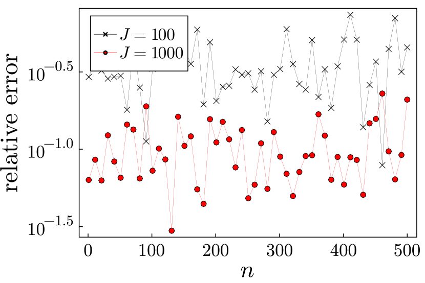
(a) Single-level, $\frac{\lvert\Theta[\bar{X}_{n}]-\widehat{\Theta}(\bm{x}_{n}^{L})\rvert}{\lvert\Theta[\bar{X}_{n}]\rvert}$

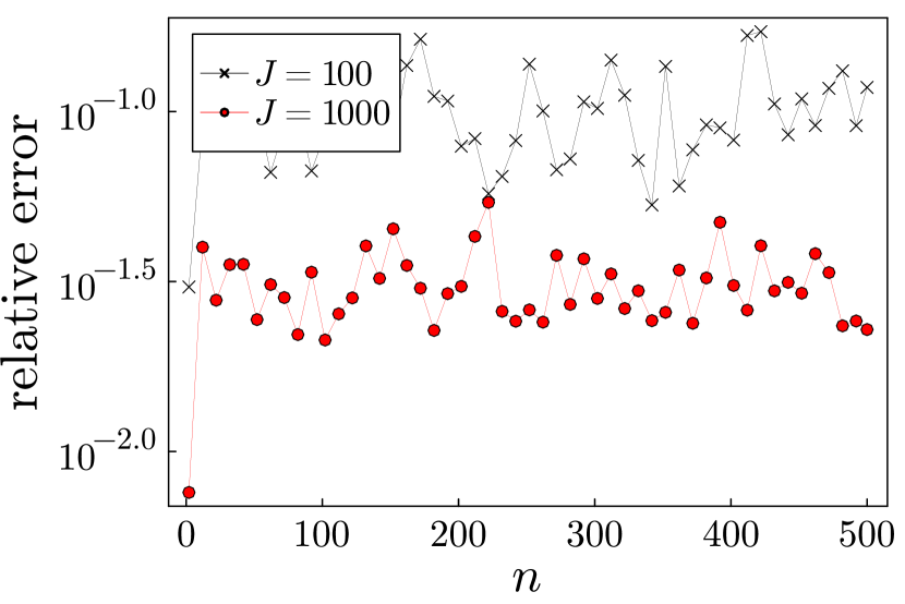
(b) Single-level, $\lvert\bar{u}_{n}^{L}-u_{n}^{L}\rvert/\lvert\bar{u}_{n}^{L}\rvert$

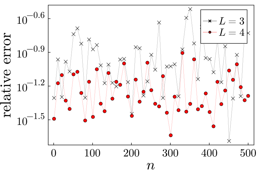
(c) Multilevel, $\frac{\lvert\Theta[\bar{X}_{n}]-\widehat{\Theta}^{\mathrm{ML}}(\bm{x}_{n}^{\mathrm{ML}})\rvert}{\lvert\Theta[\bar{X}_{n}]\rvert}$

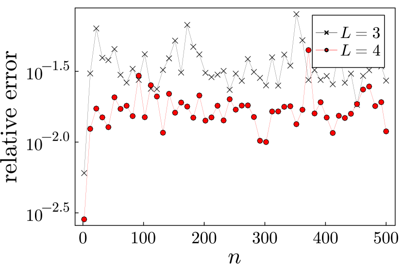
(d) Multilevel, $\lvert\bar{u}_{n}^{L}-u_{n}^{L}\rvert/\lvert\bar{u}_{n}^{L}\rvert$

Figure 1: EKS errors on the statistic and particle paths compared to the mean field.

For IPMs such as EKI and EKS (Examples 1.2 and 1.3), the goal is to approximate the mean-field particle distribution for $n\rightarrow\infty$. In practice, a finite truncation must be made. This can be achieved by simulating the IPM as in Section 3, but with an added dependence of the number of time steps $N$ on the error tolerance. We detail the differences in methodology, cost, and accuracy. In this section, we assume that $\lVert Q_{N}^{{\mathrm{ML}}}-\bar{q}_{N}\rVert_{p}\lesssim_{\epsilon}\epsilon$ without the $\log_{\rho}(\epsilon^{-1})^{N}$ factor – see Remark 4.6 for a discussion and Section 8 for supporting numerical tests.

Denote by $r$ a bound for the convergence of the QoI of the mean-field in time:

(52) $$\lvert\bar{q}_{N}-\bar{q}_{\infty}\rvert\leq r(N).$$

Let $Q_{N}$ be equal to either $Q_{N}^{L}$ or $Q_{N}^{{\mathrm{ML}}}$, depending on the context. Suppose we want the error $\lVert Q_{N}-\bar{q}_{\infty}\rVert_{p}$ to be at most asymptotically proportional to some ${\mathtt{tol}}>0$:

(53) $$\lVert Q_{N}-\bar{q}_{N}\rVert_{p}+\lvert\bar{q}_{N}-\bar{q}_{\infty}\rvert\lesssim{\mathtt{tol}}.$$

We then adapt our algorithms from Sections 3.1 and 3.3 to simulate not until a fixed $N$, but until $N({\mathtt{tol}})=r^{-1}({\mathtt{tol}})$. This prompts us to make the $N$-dependence in the asymptotic inequality Eq. 33 or Eq. 36 explicit; define a function $s$ such that

(54) $$\lVert Q_{N}-\bar{q}_{N}\rVert_{p}\lesssim s(N)\epsilon.$$

This means that we can choose (with “ih” or “fh” denoting infinite or fixed horizons)

(55) $$\epsilon_{\mathrm{ih}}({\mathtt{tol}})\eqsim\frac{{\mathtt{tol}}}{s(r^{-1}({\mathtt{tol}}))}\quad\text{with}\quad\mathrm{Cost}_{\mathrm{ih}}\eqsim r^{-1}({\mathtt{tol}})\mathrm{Cost}_{\mathrm{fh}}\Bigl{(}\frac{{\mathtt{tol}}}{s(r^{-1}({\mathtt{tol}}))}\Bigr{)}$$

and, through Eq. 54, achieve the desired $\lVert Q_{N}-\bar{q}_{N}\rVert_{p}\lesssim{\mathtt{tol}}$. Notably, if $s(N)\eqsim 1$ (i.e., if the constant hidden in Eq. 33 or Eq. 36 is $N$-independent), we can choose $\epsilon_{\mathrm{ih}}={\mathtt{tol}}$ and the cost for an infinite-horizon IPM is $r^{-1}({\mathtt{tol}})$ times the fixed-horizon cost.

Deriving $s$ for specific IPMs is outside the scope of this paper, but we will study one case numerically. Consider EKS (Example 1.3) applied to the first test problem from Section 8.2, with $N=500$ and $J\in\{100,1000\}$ (single-level) or $L\in\{3,4\}$ (multilevel). The constant hidden in Eq. 33 comes from those in Eq. 45, which pertain to the distance between the exact parameter $\Theta[\bar{X}_{n}]$ and the sample statistic $\widehat{\Theta}(\bm{x}_{n}^{L})$, and that between the particle $\bar{u}_{n}^{L}$ using the exact parameter and a correlated particle $u_{n}^{L}$ using the statistic. An analogous relation exists between Eq. 36 and the bounds Eq. 49. After approximating $\Theta[\bar{X}_{n}]$ by using $10^{5}$ particles, we plot in Fig. 1 these quantities evolving over time $n$. For this IPM and this example, all graphs plateau after a short transition period, at a level proportional to $\epsilon$. This suggests that, for EKS and this forward model, $s(N)\eqsim 1$, which indicates time-uniform errors. This situation is similar to that of multilevel particle filters [29], whose theoretical error bounds are time-dependent, while numerical tests show time-uniformity.

8 Scaling experiments

In this section, we set out to corroborate our single-level and multilevel asymptotic cost-to-error bounds under the assumptions in Section 4.1. First, in Section 8.1, we consider state estimation of an Ornstein–Uhlenbeck process in one and in twenty dimensions, by use of a filtering IPM with a fixed number of discrete time steps. Then we move to Bayesian inverse problems in Section 8.2, and apply various infinite-horizon IPMs to state estimation in an ODE, a set-up with the time-dependent heat equation, and Darcy flow. We show empirically that our analytic cost-to-error rate still holds. Finally, we discuss and interpret our results in Section 8.3. Our code is open-source and can be found in the repository

https://gitlab.kuleuven.be/numa/public/paper-code-mlipm.

8.1 IPMs with a fixed number of time steps

Our rigorous convergence results in Theorems 4.2 and 4.4 apply to IPMs with a fixed number of time steps. One such method, the ensemble Kalman filter, is extensively studied in [23], whose MLEnKF algorithm matches our method when applied to the EnKF. Hence, we do not repeat their experiments; we instead study an alternative that can now also be simulated in a multilevel way within our framework. It is introduced in Example 8.1.

Example 8.1 (Deterministic ensemble Kalman filter).

The work [37] proposes the deterministic ensemble Kalman filter (DEnKF) as an alternative to the EnKF from Example 1.1. It uses the dynamics

(56) $$u_{n+1}^{j}=(I-\frac{1}{2}K_{n}H)(\mathcal{G}(u_{n}^{j})-E_{J}(\bm{g}_{n}))+E_{J}(\bm{g}_{n})+K_{n}(y_{n+1}-H\mathcal{G}(u_{n}^{j})),$$

where $K_{n}$ is the Kalman gain introduced in Example 1.1.

An Ornstein–Uhlenbeck process

We mean to estimate the state of a $d_{u}$-dimensional Ornstein–Uhlenbeck process with parameters $\theta$ and $\sigma$, described by

(57) $$\differential u=-\theta u\differential t+\sigma\differential W,\qquad u(0)=\begin{bmatrix}1,1,\ldots,1\end{bmatrix}^{\mathstrut\scriptscriptstyle{\top}}\in\mathbb{R}^{d_{u}},$$

based on noisy measurements of $u$. We will consider two cases: $d_{u}=1$ and $d_{u}=20$. The one-dimensional variant of this problem was also used as an example in [23]. When $d_{u}=1$, we choose scalar parameters $\theta=\sigma=0.3$; when $d_{u}=20$, we set

(58) $$\theta=\frac{1}{10}\left[\begin{smallmatrix}3&1&&\\ 1&\mathinner{\mathchoice{\vbox{\kern 2.58612pt\vbox to6.1833pt{\offinterlineskip\hbox{$\displaystyle\mathpunct{.}$}\vfill\hbox{$\displaystyle\mathpunct{\kern 1.94444pt}\mathpunct{.}$}\vfill\hbox{$\displaystyle\mathpunct{\kern 1.94444pt}\mathpunct{\kern 1.94444pt}\mathpunct{.}$}}}}{\vbox{\kern 2.58612pt\vbox to6.1833pt{\offinterlineskip\hbox{$\textstyle\mathpunct{.}$}\vfill\hbox{$\textstyle\mathpunct{\kern 1.94444pt}\mathpunct{.}$}\vfill\hbox{$\textstyle\mathpunct{\kern 1.94444pt}\mathpunct{\kern 1.94444pt}\mathpunct{.}$}}}}{\vbox{\kern 2.04362pt\vbox to4.79498pt{\offinterlineskip\hbox{$\scriptstyle\mathpunct{.}$}\vfill\hbox{$\scriptstyle\mathpunct{\kern 1.36111pt}\mathpunct{.}$}\vfill\hbox{$\scriptstyle\mathpunct{\kern 1.36111pt}\mathpunct{\kern 1.36111pt}\mathpunct{.}$}}}}{\vbox{\kern 1.68195pt\vbox to3.8694pt{\offinterlineskip\hbox{$\scriptscriptstyle\mathpunct{.}$}\vfill\hbox{$\scriptscriptstyle\mathpunct{\kern 0.97221pt}\mathpunct{.}$}\vfill\hbox{$\scriptscriptstyle\mathpunct{\kern 0.97221pt}\mathpunct{\kern 0.97221pt}\mathpunct{.}$}}}}\mkern 3.0mu}&\mathinner{\mathchoice{\vbox{\kern 2.58612pt\vbox to6.1833pt{\offinterlineskip\hbox{$\displaystyle\mathpunct{.}$}\vfill\hbox{$\displaystyle\mathpunct{\kern 1.94444pt}\mathpunct{.}$}\vfill\hbox{$\displaystyle\mathpunct{\kern 1.94444pt}\mathpunct{\kern 1.94444pt}\mathpunct{.}$}}}}{\vbox{\kern 2.58612pt\vbox to6.1833pt{\offinterlineskip\hbox{$\textstyle\mathpunct{.}$}\vfill\hbox{$\textstyle\mathpunct{\kern 1.94444pt}\mathpunct{.}$}\vfill\hbox{$\textstyle\mathpunct{\kern 1.94444pt}\mathpunct{\kern 1.94444pt}\mathpunct{.}$}}}}{\vbox{\kern 2.04362pt\vbox to4.79498pt{\offinterlineskip\hbox{$\scriptstyle\mathpunct{.}$}\vfill\hbox{$\scriptstyle\mathpunct{\kern 1.36111pt}\mathpunct{.}$}\vfill\hbox{$\scriptstyle\mathpunct{\kern 1.36111pt}\mathpunct{\kern 1.36111pt}\mathpunct{.}$}}}}{\vbox{\kern 1.68195pt\vbox to3.8694pt{\offinterlineskip\hbox{$\scriptscriptstyle\mathpunct{.}$}\vfill\hbox{$\scriptscriptstyle\mathpunct{\kern 0.97221pt}\mathpunct{.}$}\vfill\hbox{$\scriptscriptstyle\mathpunct{\kern 0.97221pt}\mathpunct{\kern 0.97221pt}\mathpunct{.}$}}}}\mkern 3.0mu}\\ &\mathinner{\mathchoice{\vbox{\kern 2.58612pt\vbox to6.1833pt{\offinterlineskip\hbox{$\displaystyle\mathpunct{.}$}\vfill\hbox{$\displaystyle\mathpunct{\kern 1.94444pt}\mathpunct{.}$}\vfill\hbox{$\displaystyle\mathpunct{\kern 1.94444pt}\mathpunct{\kern 1.94444pt}\mathpunct{.}$}}}}{\vbox{\kern 2.58612pt\vbox to6.1833pt{\offinterlineskip\hbox{$\textstyle\mathpunct{.}$}\vfill\hbox{$\textstyle\mathpunct{\kern 1.94444pt}\mathpunct{.}$}\vfill\hbox{$\textstyle\mathpunct{\kern 1.94444pt}\mathpunct{\kern 1.94444pt}\mathpunct{.}$}}}}{\vbox{\kern 2.04362pt\vbox to4.79498pt{\offinterlineskip\hbox{$\scriptstyle\mathpunct{.}$}\vfill\hbox{$\scriptstyle\mathpunct{\kern 1.36111pt}\mathpunct{.}$}\vfill\hbox{$\scriptstyle\mathpunct{\kern 1.36111pt}\mathpunct{\kern 1.36111pt}\mathpunct{.}$}}}}{\vbox{\kern 1.68195pt\vbox to3.8694pt{\offinterlineskip\hbox{$\scriptscriptstyle\mathpunct{.}$}\vfill\hbox{$\scriptscriptstyle\mathpunct{\kern 0.97221pt}\mathpunct{.}$}\vfill\hbox{$\scriptscriptstyle\mathpunct{\kern 0.97221pt}\mathpunct{\kern 0.97221pt}\mathpunct{.}$}}}}\mkern 3.0mu}&\mathinner{\mathchoice{\vbox{\kern 2.58612pt\vbox to6.1833pt{\offinterlineskip\hbox{$\displaystyle\mathpunct{.}$}\vfill\hbox{$\displaystyle\mathpunct{\kern 1.94444pt}\mathpunct{.}$}\vfill\hbox{$\displaystyle\mathpunct{\kern 1.94444pt}\mathpunct{\kern 1.94444pt}\mathpunct{.}$}}}}{\vbox{\kern 2.58612pt\vbox to6.1833pt{\offinterlineskip\hbox{$\textstyle\mathpunct{.}$}\vfill\hbox{$\textstyle\mathpunct{\kern 1.94444pt}\mathpunct{.}$}\vfill\hbox{$\textstyle\mathpunct{\kern 1.94444pt}\mathpunct{\kern 1.94444pt}\mathpunct{.}$}}}}{\vbox{\kern 2.04362pt\vbox to4.79498pt{\offinterlineskip\hbox{$\scriptstyle\mathpunct{.}$}\vfill\hbox{$\scriptstyle\mathpunct{\kern 1.36111pt}\mathpunct{.}$}\vfill\hbox{$\scriptstyle\mathpunct{\kern 1.36111pt}\mathpunct{\kern 1.36111pt}\mathpunct{.}$}}}}{\vbox{\kern 1.68195pt\vbox to3.8694pt{\offinterlineskip\hbox{$\scriptscriptstyle\mathpunct{.}$}\vfill\hbox{$\scriptscriptstyle\mathpunct{\kern 0.97221pt}\mathpunct{.}$}\vfill\hbox{$\scriptscriptstyle\mathpunct{\kern 0.97221pt}\mathpunct{\kern 0.97221pt}\mathpunct{.}$}}}}\mkern 3.0mu}&\\ &&1&3\end{smallmatrix}\right]\in\mathbb{R}^{20\times 20}\quad\mathrm{and}\quad\sigma=\frac{1}{10}\left[\begin{smallmatrix}3&&&\\ &\mathinner{\mathchoice{\vbox{\kern 2.58612pt\vbox to6.1833pt{\offinterlineskip\hbox{$\displaystyle\mathpunct{.}$}\vfill\hbox{$\displaystyle\mathpunct{\kern 1.94444pt}\mathpunct{.}$}\vfill\hbox{$\displaystyle\mathpunct{\kern 1.94444pt}\mathpunct{\kern 1.94444pt}\mathpunct{.}$}}}}{\vbox{\kern 2.58612pt\vbox to6.1833pt{\offinterlineskip\hbox{$\textstyle\mathpunct{.}$}\vfill\hbox{$\textstyle\mathpunct{\kern 1.94444pt}\mathpunct{.}$}\vfill\hbox{$\textstyle\mathpunct{\kern 1.94444pt}\mathpunct{\kern 1.94444pt}\mathpunct{.}$}}}}{\vbox{\kern 2.04362pt\vbox to4.79498pt{\offinterlineskip\hbox{$\scriptstyle\mathpunct{.}$}\vfill\hbox{$\scriptstyle\mathpunct{\kern 1.36111pt}\mathpunct{.}$}\vfill\hbox{$\scriptstyle\mathpunct{\kern 1.36111pt}\mathpunct{\kern 1.36111pt}\mathpunct{.}$}}}}{\vbox{\kern 1.68195pt\vbox to3.8694pt{\offinterlineskip\hbox{$\scriptscriptstyle\mathpunct{.}$}\vfill\hbox{$\scriptscriptstyle\mathpunct{\kern 0.97221pt}\mathpunct{.}$}\vfill\hbox{$\scriptscriptstyle\mathpunct{\kern 0.97221pt}\mathpunct{\kern 0.97221pt}\mathpunct{.}$}}}}\mkern 3.0mu}&&\\ &&\mathinner{\mathchoice{\vbox{\kern 2.58612pt\vbox to6.1833pt{\offinterlineskip\hbox{$\displaystyle\mathpunct{.}$}\vfill\hbox{$\displaystyle\mathpunct{\kern 1.94444pt}\mathpunct{.}$}\vfill\hbox{$\displaystyle\mathpunct{\kern 1.94444pt}\mathpunct{\kern 1.94444pt}\mathpunct{.}$}}}}{\vbox{\kern 2.58612pt\vbox to6.1833pt{\offinterlineskip\hbox{$\textstyle\mathpunct{.}$}\vfill\hbox{$\textstyle\mathpunct{\kern 1.94444pt}\mathpunct{.}$}\vfill\hbox{$\textstyle\mathpunct{\kern 1.94444pt}\mathpunct{\kern 1.94444pt}\mathpunct{.}$}}}}{\vbox{\kern 2.04362pt\vbox to4.79498pt{\offinterlineskip\hbox{$\scriptstyle\mathpunct{.}$}\vfill\hbox{$\scriptstyle\mathpunct{\kern 1.36111pt}\mathpunct{.}$}\vfill\hbox{$\scriptstyle\mathpunct{\kern 1.36111pt}\mathpunct{\kern 1.36111pt}\mathpunct{.}$}}}}{\vbox{\kern 1.68195pt\vbox to3.8694pt{\offinterlineskip\hbox{$\scriptscriptstyle\mathpunct{.}$}\vfill\hbox{$\scriptscriptstyle\mathpunct{\kern 0.97221pt}\mathpunct{.}$}\vfill\hbox{$\scriptscriptstyle\mathpunct{\kern 0.97221pt}\mathpunct{\kern 0.97221pt}\mathpunct{.}$}}}}\mkern 3.0mu}&\\ &&&3\end{smallmatrix}\right]\in\mathbb{R}^{20\times 20}.$$

Noisy observations $y_{n}$ of the process Eq. 57 are available at times $t_{n}=n$. Let us call $\mathcal{G}$ the operator that evolves Eq. 57 exactly over a time interval of $1$. Then,

(59) $$u_{n+1} =\mathcal{G}(u_{n}),$$

$$y_{n} =u_{n}+\eta_{n},$$

with measurement noise $\eta_{n}\sim N(0,\Gamma)$. We assume that computing an exact solution to Eq. 57 is infeasible and introduce approximations $\{\mathcal{G}^{\ell}\}_{\ell}$, which are Milstein discretizations at resolutions $h^{\ell}=2^{-\ell}$. In other words, $\mathcal{G}^{\ell}(u_{n})=u_{n,2^{\ell}}$, where

(60) $$\widehat{u}_{n,k+1}^{\ell}=(1-h^{\ell}\theta)\widehat{u}_{n,k}^{\ell}+\sigma\sqrt{h^{\ell}}\Delta W^{\ell}_{n,k}\qquad\text{and}\qquad\widehat{u}_{n,0}^{\ell}=u_{n}.$$

To ensure correlation between a pair of particles on level $\ell$, the Brownian increments

(61) $$\Delta W^{\ell}_{n,k}=W(t_{n}+(k+1)h^{\ell})-W(t_{n}+kh^{\ell})$$

are computed from the same Brownian path $W$. The cost of Eq. 60 scales with $\ell$ as

(62) $$\mathrm{Cost}(\mathcal{G}^{\ell})=2^{\ell}\mathrm{Cost}(\mathcal{G}^{0}).$$

Therefore $\gamma=1$. We also have $\beta=2$ (see [19, 23]). For the QoI of the filtering distribution, we choose the particle mean. As a gold standard, a highly accurate approximation of the expected value of the mean-field particle distribution is obtained by averaging the means of $10$ large-scale ($J=10^{4}$) single-level simulations using a very accurate forward model ($L=12$). We consider the root-mean-square error (RMSE) between $10$ independent ensemble means and this gold standard.

Figure 2: RMSE as a function of relative cost (total cost compared to the cost of $\mathcal{G}^{0}$) for state estimation of an Ornstein–Uhlenbeck process with DEnKF.

The cost of simulating a single-level or multilevel ensemble can be quantified as

(63a) $$\mathrm{Cost}^{\mathrm{SL}} =J2^{L\gamma}N\mathrm{Cost}(\mathcal{G}^{0}),$$

(63b) $$\mathrm{Cost}^{\mathrm{ML}} =\Bigl{(}J_{0}+\sum\nolimits_{\ell=1}^{L}J_{\ell}(2^{\ell\gamma}+2^{(\ell-1)\gamma})\Bigr{)}N\mathrm{Cost}(\mathcal{G}^{0}).$$

In Fig. 2, this cost is plotted against the RMSE for a number of both single-level and multilevel experiments. The values of $L$, $J$, and $J_{\ell}$ are chosen in accordance with the scaling laws set out in Eq. 32 and Eq. 35. From $\beta$ and $\gamma$, by Theorems 4.2 and 4.4, we predict $\mathrm{RMSE}\lesssim(\mathrm{Cost}^{\mathrm{SL}})^{-1/3}$ for single-level and $\mathrm{RMSE}\lesssim(\mathrm{Cost}^{\mathrm{ML}})^{-1/2}$ for multilevel. The figure shows that the multilevel scheme adheres closely to this rate at all time points $N\in\{5,20,50\}$. The single-level method initially converges somewhat faster than its expected rate, but later decreases its slope to $-1/3$.

8.2 IPMs with an infinite number of time steps

Section 7 discussed applying our single- and multilevel simulation algorithms to IPMs whose time horizon grows as the required accuracy increases. In this subsection, we test this idea numerically using the EKI and EKS methods introduced earlier. The first example problem will use the base versions of these methods. For the other two examples, to stabilize and accelerate both the single-level and the multilevel methods, we use the adaptive time steps introduced in [30] and also used in [17]. This step is defined as $\tau_{n}=\alpha/(\lvert D_{n}\rvert_{F}+\varepsilon)$ for some ensemble-dependent matrix $D_{n}$ encoding the distance from the particles to each other and to the observation. Here, we denoted by $\lvert\kern 2.0pt\cdot\kern 2.0pt\rvert_{F}$ the Frobenius norm. We compute $\tau_{n}$ for each level separately, and use their minimum.

We will choose the parameters of our multilevel interacting-particle methods as if $s(N)\eqsim 1$ in Eq. 54, which is what was observed for EKS in Fig. 1. Based on the match between experiments and the expected cost-to-error relation Eq. 55, we can then assess the accuracy of this assumption. The bound $r(N)$ for the convergence of EKI in time is estimated as $r(N)\eqsim N^{-1}$, motivated by [26]. EKS and adaptive versions of both methods converges exponentially [17], but since the base of this exponential is unknown, we choose the conservative $r(N)\eqsim N^{-1/\delta}$ (with $\delta=0.1$).

Low-dimensional Bayesian inversion: A simple ODE

As a first problem, we consider the identification of the parameter $u=[u_{1},u_{2}]^{\mathstrut\scriptscriptstyle{\top}}$ in the linear ODE

(64) $$v^{\prime}(t)=u_{2}v(t),\qquad v(0)=u_{1}$$

given the observation, influenced by measurement noise $\eta\sim\mathcal{N}(0,\Gamma)$,

(65) $$y=\mathcal{G}(u)+\eta\coloneqq\Bigl{[}\begin{smallmatrix}v(0.25)\\ v(0.75)\end{smallmatrix}\Bigr{]}+\eta.$$

While the solution $v(t)=\exp(u_{2}t)u_{1}$ is trivial to compute, we will purport for this exploratory example that it must be approximated numerically with a hierarchy of implicit-Euler schemes with resolutions $h^{\ell}\eqsim 2^{2+\ell/2}$, such that $\beta=1$ and $\gamma=1/2$:

(66) $$\mathcal{G}^{\ell}(u)=\Bigl{[}\begin{smallmatrix}v^{\ell}(0.25)\\ v^{\ell}(0.75)\end{smallmatrix}\Bigr{]}\qquad\mathrm{where}\qquad v^{\ell}(t)=u_{1}(1-h^{\ell}u_{2})^{-t/h^{\ell}}.$$

We use the observed value $y=[0.85,0.65]^{\mathstrut\scriptscriptstyle{\top}}$ and a noise covariance $\Gamma=0.5^{2}I_{2}$. The prior for EKS is set to a zero-centered Gaussian with covariance $\Gamma_{0}=I_{2}$. The initial ensemble is sampled as $u_{1}\sim\mathcal{N}(1,0.25)$ and $u_{2}\sim\mathcal{U}([-1,0])$. We apply two IPMs to the problem of recovering $u$ given $y$: EKI with time steps $\tau_{n}=1$ and EKS with $\tau_{n}=0.001$ for $n\leq 50$ and $\tau_{n}=0.1$ otherwise. By Eq. 55, we expect single- and multilevel cost-to-error relations of $\mathrm{RMSE}\lesssim(\mathrm{Cost}^{\mathrm{SL}})^{-1/4}$ and $\mathrm{RMSE}\lesssim(\mathrm{Cost}^{\mathrm{ML}})^{-1/3}$ for EKI, and of $\mathrm{RMSE}\lesssim(\mathrm{Cost}^{\mathrm{SL}})^{-1/(3+\delta)}$ and $\mathrm{RMSE}\lesssim(\mathrm{Cost}^{\mathrm{ML}})^{-1/(2+\delta)}$ for EKS.

Figure 3: RMSE as a function of relative cost (total cost compared to the cost of $\mathcal{G}^{0}$) for inversion of a low-dimensional ODE problem. Note that the theoretical multilevel rate hides a logarithmic factor, which is visible in the computational results (which otherwise match the theorized rates well).

When $L$, $J$, $\{J_{\ell}\}_{\ell}$, and $N$ are chosen according to our scaling laws Eq. 32, Eq. 35, and $N=r^{-1}(\epsilon)$, Fig. 3 shows that these asymptotic rates are matched in practice. A non-asymptotic comparison of single- and multilevel IPMs should not be made on the basis of these experiments; see the discussion in Section 8.3.

Higher-dimensional Bayesian inversion: A heat equation

Figure 4: RMSE as a function of relative cost (total cost compared to the cost of $\mathcal{G}^{0}$) for inversion of a higher-dimensional time-dependent heat problem. Note, as in Fig. 3, the logarithmic factor visible in the multilevel results.

A first higher-dimensional inverse problem we consider is concerned with recovering source terms in a time-dependent heat equation, based on noisy measurements. The physical set-up consists of the one-dimensional domain $x\in[0,20]$ with boundaries of fixed temperature $\theta_{\mathrm{b}}=293$. All non-boundary integer positions are fitted with heat point sources or temperature sensors; sensors at the odd positions and sources at the even ones. The sources are modelled as Dirac deltas of unknown but time-invariant magnitude. At time $t=0$, the entire domain has temperature $\theta(x,0)=\theta_{\mathrm{b}}=293$ and the sources are activated. The sensors take measurements at $t=5$ and at $t=10$. We thus have $d_{u}=9$ unknown sources and $d_{g}=20$ measurements.

The forward problem $\mathcal{G}$ is determining $\theta(x^{*},t^{*})$ at the $10$ sensor positions $x^{*}$ at each of $2$ measurement times $t^{*}$, given that $\theta$ solves the time-dependent heat equation

(67) $$\partial_{t}\theta=\partial_{xx}\theta+f,$$

where the source $f$ is the input. Approximations $\mathcal{G}^{\ell}$ solve Eq. 67 with a backward-time centered-space scheme. We ensure that there are always spatial discretization points on the sources and sensors, and temporal ones on the measurement times. With a temporal step $h_{t}^{\ell}\eqsim 2^{(4+\ell)/2}$ and a spatial step $h_{x}^{\ell}\eqsim 2^{(18+\ell)/4}$, we obtain $\beta=1$ and $\gamma=3/4$. We model a noise covariance $\Gamma=I$ and, for EKS, use a zero-centered prior with covariance $\Gamma_{0}=10^{2}I$. The observation is generated by sampling the prior, solving the forward model at high resolution, and adding noise from $\mathcal{N}(0,\Gamma)$.

We apply EKI and EKS to this problem, both with adaptive time steps; we choose $(\alpha,\varepsilon)=(1,0.001)$. For this higher-dimensional problem, too, Fig. 4 reveals good correspondence between the theoretical convergence rates and experimental results.

Higher-dimensional Bayesian inversion: Darcy flow

Figure 5: Measurement points in the pressure fields of the Darcy flow problem

Within the literature on Bayesian inversion, the Darcy flow test problem is a classical one (see, e.g., [17, 26]). On the two-dimensional spatial domain $[0,1]^{2}$, our forward model computes the map of the positive permeability field $a(x,u)$ of a porous medium to the pressure field $p(x)$ that satisfies

(68) $$-\nabla\cdot(a(x,u)\nabla p(x)) =f(x) \text{if $x\in[0,1]^{2}$},$$

$$p(x) =0 x\in\partial[0,1]^{2}$$ if .

We set $f(x_{1},x_{2})=1000\exp(x_{1}+x_{2})$. The parameter $u$ to the model consists of the first $d_{u}=16$ terms in the Karhunen-Loève (KL) expansion

(69) $$\log a(x,u)=\sum_{k\in\mathbb{Z}^{2}\backslash\{(0,0)\}}u_{k}\sqrt{\lambda_{k}}\phi_{k}(x),$$

where the eigenpairs are [26]

(70) $$\phi_{k}(x)=\begin{cases}\sqrt{2}\cos(\pi k_{1}x_{1})&\text{if $k_{2}=0$},\\ \sqrt{2}\cos(\pi k_{2}x_{2})&\text{if $k_{1}=0$},\\ 2\cos(\pi k_{1}x_{1})\cos(\pi k_{2}x_{2})&\text{otherwise},\end{cases}$$

and

(71) $$\lambda_{k}=(\pi^{2}(k_{1}^{2}+k_{2}^{2})+\tau^{2})^{-d},$$

and which, for the purpose of truncation, is ordered by descending size of the eigenvalues $\lambda_{k}$. We model $a(x,u)$ as a log-normal random field with covariance $(-\Delta+\tau^{2})^{-d}$ that corresponds to a standard normal prior on the coefficients $u_{k}$. The output of the forward model consists of $p$ evaluated on 49 equispaced points (as shown in Fig. 5), and the noise added has covariance $\Gamma=0.01I$. EKS uses a zero-centered prior with covariance $\Gamma_{0}=I$.

Using central differences for the derivatives in Eq. 68, with steps $h^{\ell}\eqsim 2^{(13+\ell)/4}$, yields a forward model with $\beta=1$ and $\gamma=1/2$. We show experimental results, next to the theoretically expected rates, in Fig. 6. As with the other examples, the correspondence between the two is good.

Figure 6: RMSE as a function of relative cost (total cost compared to the cost of $\mathcal{G}^{0}$) for inversion of a higher-dimensional Darcy flow problem. Note, as in Fig. 3, the logarithmic factor visible in the multilevel results.

8.3 Discussion

Theorems 4.2 and 4.4 imply that, for IPMs in our framework with a fixed number of time steps, our multilevel simulation algorithm Eq. 24 asymptotically enjoys faster convergence than the more straightforward single-level algorithm Eq. 17. The numerical scaling tests conducted in Sections 8.1 and 8.2 demonstrate that these rates are accurate. These conclusions hold for the whole range of IPMs studied, and for both low- and higher-dimensional problems.

We stress that our theory only provides asymptotic rates and does not result in guidelines for selecting the constants in Eq. 32, Eq. 35, or – in the case of non-fixed time horizons – the function $r(N)$. We give the following comments.

• Changing these constants should, in general, shift the convergence graphs without changing their slopes.

• Since the constants are not optimized, we cannot compare the performance of single- and multilevel simulation for a fixed cost in a meaningful way. Their relative positions depend on these chosen values for these constants, which can be found in our code repository. However, the convergence rates can be compared, and those are the focus of this article.

• To improve the performance of our multilevel strategy in practice, adaptive or non-adaptive schemes to tune these constants are vital. We comment further on this aspect in the future-work part of Section 9.

These limitations are also present in the experiments that are performed in [9, 23]. We intend to tackle this important aspect of multilevel interacting-particle methods in a future paper.

9 Conclusions

We have proposed a general framework for interacting-particle methods, which includes many popular methods used for filtering, optimization, and sampling. Two classes of methods are identified within this framework: those with a fixed and those with an infinite number of discrete time steps. The setting we considered is that where the dynamics of the IPM include an intractable forward model $\mathcal{G}$, to which an approximation hierarchy $\{\mathcal{G}^{\ell}\}_{\ell}$ is available.

For IPMs in the framework, we have described and analyzed two methods that allow a numerical approximation of the particle density. The first is a standard Monte Carlo simulation that uses a finite ensemble of particles. As an alternative, we have developed a generalization of the multilevel Monte Carlo approach proposed for the ensemble Kalman filter in [9, 23], which we call single-ensemble MLMC. This algorithm uses a single, globally coupled ensemble whose base-level particles and higher-level correction pairs use various different levels $\ell$. The MLMC methodology is then used to estimate the interaction term at each time step.

For IPMs with a fixed number of time steps, we formulated Sections 4.1, 4.1, and 4.1, under which rigorous convergence results were shown in Theorems 4.2 and 4.4. These bounds suggest that single-ensemble MLMC always asymptotically outperforms standard Monte Carlo. For a variety of IPMs, we have shown that our assumptions hold, such that the convergence bounds are valid. Experiments suggest that the convergence rates implied by the bounds are accurate. Despite these results, two open questions remain.

• The factor $\log_{\rho}(\epsilon^{-1})^{N}$ in the upper bound Eq. 36 is fortunately absent in practice, as discussed in Remark 4.6. An upper bound for single-ensemble multilevel interacting-particle methods that does not contain this factor would improve the theoretical foundation of the MLMC approach. In this context, we also refer to the discussion in [9, Remark 5].

• Next to this $(\epsilon,N)$-dependent factor, the asymptotic bounds in Theorems 4.2 and 4.4 obscure a constant that is potentially $N$-dependent. Knowing more about this constant for a given IPM is crucial when the number of time steps depends on the required accuracy (see Section 7). Fortunately, our tests in Sections 7 and 8 suggest that these effects can be negligible in practice; [23, p. 1833] draws similar conclusions about the EnKF.

There are many interesting directions for further research in three main categories.

• Theoretical. The two open questions above require more theoretical work to settle. In addition, theory that suggests good quantitative choices for $\{J_{\ell}\}_{\ell}$, as opposed to the proportional rates in Eq. 35, may enhance performance.

• Algorithmic. For IPMs with an $\epsilon$-dependent horizon, it may be feasible to design a single-ensemble MLMC algorithm where only the fine-level particles must take more time steps for increased accuracy. In addition, for problems with high- or infinite-dimensional parameters or data, an extension of our methodology can be developed that uses level-dependent dimensions. The multilevel EnKF in [9] already deals with infinite-dimensional parameters.

• Numerical. The MLIPMs developed in this paper should be compared to other, potentially algorithm-specific, MLMC approaches. For an effective comparison, optimized techniques to select the number of particles on each level (either adaptive or theory-based) are first needed.

In addition, this paper lays a clear path for developing multilevel simulation methods for many other interacting-particle methods that have been proposed in the literature. If Sections 4.1, 4.1, and 4.1 hold for the specific forward model, dynamics, and interaction term, then the algorithm Eq. 24–Eq. 26 can be used and Theorem 4.4 applies.

Appendix A Proofs about specific IPMs

In this appendix, we give proofs about various interacting-particle methods and parameter/statistic pairs. This links the IPMs given throughout the text to the framework detailed in Section 3 – and, more specifically, to Sections 4.1 and 4.1. Section A.1 discusses parameters and statistics, after which Section A.2 studies the IPM dynamics themselves.

A.1 Parameters and statistics

We start by proving that Section 4.1 holds for two parameter/statistic pairs used in most IPMs mentioned in this text: the (sample) mean and the (sample) covariance. We then discuss whether a similar result holds for self-normalized weighted variants.

Lemma A.1.

When the parameter $\Theta[\cdot]$ is the expectation $\mathbb{E}[\cdot]$ and the sample statistic $\widehat{\Theta}(\cdot)$ is the sample mean $E(\cdot)$, Section 4.1 is satisfied.

Proof A.2.

We first deal with Section 4.1(i):

(72) $$\lVert\widehat{\Theta}_{J}(\bm{X}_{1})-\widehat{\Theta}_{J}(\bm{X}_{2})\rVert_{p}=\Big{\lVert}\frac{1}{J}\sum\nolimits_{j=1}^{J}(X_{1,j}-X_{2,j})\Big{\rVert}_{p}\leq\lVert X_{1}-X_{2}\rVert$$

for any $p\geq 2$. For (ii), we have

(73) $$\lVert E(\bm{X}_{1})-E(\bm{X}_{2})-(\mathbb{E}[X_{1}]-\mathbb{E}[X_{2}])\rVert_{p}=\lVert E((\bm{X}_{1}-\bm{X}_{2})-\mathbb{E}[X_{1}-X_{2}])\rVert_{p}.$$

Since a sample mean is an unbiased estimator, we use Sections 2 and 2 to obtain

(74) $$\lVert E((\bm{X}_{1}-\bm{X}_{2})-\mathbb{E}[X_{1}-X_{2}])\rVert_{p}\leq 2c_{p}J^{-1/2}\lVert X_{1}-X_{2}\rVert_{p}.$$

Then, (iii) follows from (ii) by setting $X_{2}=\delta_{0}$, since $\mathbb{E}[\delta_{0}]=E(\bm{0})=0$ and $c_{\theta,2}$ is $d$-independent. Finally, (iv) is easy to check using Sections 2 and 2.

Lemma A.3.

When the parameter $\Theta[\cdot]$ is the covariance $\mathbb{C}[\cdot]$ and the sample statistic $\widehat{\Theta}(\cdot)$ is the sample covariance $C(\cdot)$, Section 4.1 is satisfied.

Proof A.4.

The proof of (i) is contained in that of [23, Lemma 3.9]; the proof of (ii) in that of [23, Lemma 3.8]. Then, (iii) and (iv) can be checked as for Lemma A.1.

A.2 Interacting-particle methods

Next, we discuss Section 4.1 for the interacting-particle methods in the paper. After giving Remarks A.5 and A.6, which are relevant for multiple IPMs, we discuss the methods one by one.

Remark A.5 (Covariance matrices).

IPMs such as the EnKF and EKS use a sample covariance matrix as statistic. A mean-field covariance or a single-level sample covariance is guaranteed to be positive semi-definite; this is important, as it ensures operations such as matrix square roots and inverses (after addition with a positive definite matrix) are well-defined. A multilevel sample covariance matrix computed by Eq. 25, on the other hand, might have negative eigenvalues. In [9, 23], this is avoided by setting all negative eigenvalues to zero in a preprocessing step. We will follow this approach and, to this end, define the operator

(75) $$I^{+}(M)=\sum\nolimits_{\lambda_{k}\geq 0}\lambda_{k}q_{k}q_{k}^{\mathstrut\scriptscriptstyle{\top}}\qquad\text{with $\{(\lambda_{k},q_{k})\}_{k}$ the eigenpairs of $M$},$$

which can be freely incorporated into existing dynamics where needed. Indeed, when applied to sample covariance matrices in the single-level algorithm, it is the identity operator. In the multilevel context, in ensures positive semi-definiteness.

In future work, it would be interesting to study multilevel covariance estimators that guarantee positive semi-definiteness directly, such as that of [33]. The advantage of the form Eq. 75 is that it builds on the naive multilevel estimation and thus is compatible with our framework’s estimator Eq. 25 by updating only the dynamics.

Remark A.6 (Matrix square roots).

IPMs such as EKS use the square root of the input covariance matrix $\theta$. To prove Section 4.1, $\theta_{1}$ in Eq. 29 then needs to be positive definite with its smallest eigenvalue bounded from below by some $\mu>0$, since then Corollary A.8 applies. In Sections 5 and 6, $\theta_{1}$ is always the mean-field parameter $\Theta[\bar{X}_{n}]$; thus, an additional assumption for IPMs using the square root of the covariance matrix is that the mean-field ensemble does not collapse to zero.

Theorem A.7 ([40, Corollary 4.2]).

If $M_{1},\,M_{2}\succeq 0$ and $M_{1}+M_{2}\succeq\mu I$ for some $\mu>0$, then for any symmetric norm $\Phi$, and $0<m\leq 1$,

(76) $$\lvert M_{1}^{m}-M_{2}^{m}\rvert_{\Phi}\leq(2/\mu)^{1-m}\lvert M_{1}-M_{2}\rvert_{\Phi}.$$

Corollary A.8.

From Theorem A.7 combined with Section 2 follows immediately that, if $M_{1},\,M_{2}\geq 0$ and $M_{1}\geq\mu I$ with $\mu>0$, then for all $p\geq 2$,

(77) $$\lVert\sqrt{M_{1}}-\sqrt{M_{2}}\rVert_{p}\leq\sqrt{2/\mu}\lVert M_{1}-M_{2}\rVert_{p}.$$

We are now ready to tackle the individual IPMs.

Lemma A.9.

The dynamics of the ensemble Kalman filter (EnKF; Example 1.1) and of ensemble Kalman inversion (EKI; Example 1.2) fit into the single-level framework Eq. 17 and satisfy Section 4.1.

Proof A.10.

We tackle the ensemble Kalman filter first. In the notation Eq. 17 of our framework, we have $\widehat{\Theta}_{J}(\bm{g})=C_{J}(\bm{g})$ and the EnKF uses the functions

(78) $$\Psi_{n}(u,g,\theta,\eta)=g-\theta H^{\mathstrut\scriptscriptstyle{\top}}(HI^{+}(\theta)H^{\mathstrut\scriptscriptstyle{\top}}+\Gamma)^{-1}(y_{n+1}-Hg+\sqrt{\Gamma}\eta),$$

with $I^{+}$ from Remark A.5. Define $K_{i}\coloneqq\theta_{i}H^{\mathstrut\scriptscriptstyle{\top}}(HI^{+}(\theta_{i})H^{\mathstrut\scriptscriptstyle{\top}}+\Gamma)^{-1}$; by Section 2,

(79) $$\lVert\Psi_{n}(U_{1},G_{1},\theta_{1},\eta)-\Psi_{n}(U_{2},G_{2},\Theta_{2},\eta)\rVert_{p}$$

$$\leq\lVert G_{1}-G_{2}\rVert_{p}+\lvert K_{1}\rvert\lvert H\rvert\lVert G_{1}-G_{2}\rVert_{p}+\lVert K_{1}-K_{2}\rVert_{2p}\lVert y_{n+1}-HG_{2}+\sqrt{\Gamma}\eta\rVert_{2p}.$$

Now notice that $\lvert K_{1}\rvert\leq\lvert\theta_{1}\rvert\lvert H\rvert/\gamma_{\min}$, where $\gamma_{\min}>0$ is $\Gamma$’s smallest eigenvalue. In addition, [23, Lemmas 3.3 and 3.4] together prove, in our notation, the bound $\lVert K_{1}-K_{2}\rVert_{2p}\leq\lvert H\rvert/\gamma_{\min}(1+2\lvert K_{1}\rvert\lvert H\rvert)\lVert\theta_{1}-\Theta_{2}\rVert_{2p}$. Thus Eq. 79 is bounded by

$$\Bigl{(}1+\frac{\lvert H\rvert^{2}}{\gamma_{\min}}\lvert\theta_{1}\rvert\Bigr{)}\lVert G_{1}-G_{2}\rVert_{p}+\Bigl{(}\frac{\lvert H\rvert}{\gamma_{\min}}+2\frac{\lvert H\rvert^{3}}{\gamma^{2}_{\min}}\lvert\theta_{1}\rvert\Bigr{)}\lVert y_{n+1}-HG_{2}+\sqrt{\Gamma}\eta\rVert_{2p}\lVert\theta_{1}-\Theta_{2}\rVert_{2p};$$

bounding factors with the locality conditions (e.g., $\lvert\theta_{1}\rvert\leq\lVert\Theta_{0}\rVert+d$) and Section 4.1(ii) concludes the proof for EnKF. The EKI dynamics Eq. 6 are an instance of the EnKF dynamics Eq. 3, with an enlarged state space [28]. The proof still applies.

In the rest of this section, the use of Section 2 and the final step of using the locality conditions and Section 4.1(ii) will be left implicit.

Lemma A.11.

The dynamics of the deterministic ensemble Kalman filter (DEnKF; Example 8.1) fit into the single-level framework Eq. 17 and satisfy Section 4.1.

Proof A.12.

With $(\widehat{\Theta}_{J}^{(1)}(\bm{g}),\widehat{\Theta}_{J}^{(2)}(\bm{g}))=(E_{J}(\bm{g}),C_{J}(\bm{g}))$ in Eq. 17 follows from Eq. 56 that $\Psi_{n}(u,g,\theta,\eta)=g+K(H\theta^{(1)}/2+y-3Hg/2)$ with ${K\coloneqq\theta^{(2)}H^{\mathstrut\scriptscriptstyle{\top}}(HI^{+}(\theta^{(2)})H^{\mathstrut\scriptscriptstyle{\top}}+\Gamma)^{-1}}$;

$$\lVert\Psi_{n}(U_{1},G_{1},\theta_{1},\eta)-\Psi_{n}(U_{2},G_{2},\Theta_{2},\eta)\rVert_{p}$$

$$\quad=\big{\lVert}\bigl{(}G_{1}+K_{1}\bigl{(}H\theta_{1}^{(1)}/2+y-3HG_{1}/2\bigr{)}\bigr{)}-\bigl{(}G_{2}+K_{2}\bigl{(}H\Theta_{2}^{(1)}/2+y-3HG_{2}/2\bigr{)}\bigr{)}\big{\rVert}_{p}$$

$$\quad\leq\lVert G_{1}-G_{2}\rVert_{p}+\lvert K_{1}\rvert(\lVert H(\theta_{1}^{(1)}-\Theta_{2}^{(1)})/2\rVert_{p}+\lVert 3H(G_{1}-G_{2})/2\rVert_{p})$$

$$\qquad+\lVert K_{1}-K_{2}\rVert_{2p}\lVert H\Theta_{2}^{(1)}/2+y-3HG_{2}/2\rVert_{2p}.$$

The proof can then be finished similarly to that of Lemma A.9.

Lemma A.13.

The dynamics of ensemble Kalman sampling (EKS; Example 1.3) fit into the single-level framework Eq. 17 and, if the mean-field particles do not collapse, satisfy Section 4.1.

Proof A.14.

With $\widehat{\Theta}_{J}(\bm{u},\bm{g})=(C^{uu}(\bm{u}),C^{ug}(\bm{u},\bm{g}))$, Eq. 7 can be manipulated into

(80) $$\Psi_{n}(u,g,\theta,\eta)=(I+\tau_{n}\theta^{(1)}\Gamma_{0}^{-1})^{-1}\bigl{[}u+\tau_{n}\theta^{(2)}\Gamma^{-1}(y-g)\bigr{]}+\sqrt{\rule{0.0pt}{7.5347pt}2\tau_{n}\smash[t]{I^{+}(\theta^{(1)})}}\kern 2.0pt\eta.$$

Then follows (since $\smash[t]{\lVert\Theta_{2}^{(1)}-I^{+}(\Theta_{2}^{(1)})\rVert_{p}\leq\lVert\Theta_{2}^{(1)}-\theta_{1}^{(1)}\rVert_{p}}$ similarly to [23, Lemma 3.3]):

$$\lVert\Psi_{n}(U_{1},G_{1},\theta_{1},\eta)-\Psi_{n}(U_{2},G_{2},\Theta_{2},\eta)\rVert_{p}\leq\lVert\sqrt{2\tau_{n}}\kern 2.0pt\eta\rVert_{2p}\,\lVert\sqrt{\rule{0.0pt}{8.1805pt}\smash[tb]{\theta_{1}^{(1)}}}-\sqrt{\rule{0.0pt}{8.1805pt}\smash[tb]{I^{+}(\Theta_{2}^{(1)})}}\rVert_{2p}$$

$$\qquad+\lVert(I+\tau_{n}\Theta_{2}^{(1)}\Gamma_{0}^{-1})^{-1}[U_{1}-U_{2}+\tau_{n}\theta_{1}^{(2)}\Gamma^{-1}(y-G_{1})-\tau_{n}\Theta_{2}^{(2)}\Gamma^{-1}(y-G_{2})]\rVert_{p}$$

$$\qquad+\lVert((I+\tau_{n}\theta_{1}^{(1)}\Gamma_{0}^{-1})^{-1}-(I+\tau_{n}\Theta_{2}^{(1)}\Gamma_{0}^{-1})^{-1})[U_{1}+\tau_{n}\theta_{1}^{(2)}\Gamma^{-1}(y-G_{1})]\rVert_{p}$$

$$\quad\leq 2\sqrt{2\tau_{n}/\mu}\lVert\eta\rVert_{2p}\lVert\theta_{1}^{(1)}-\Theta_{2}^{(1)}\rVert_{2p}$$

$$\qquad+\lVert U_{1}-U_{2}\rVert_{p}+\tau_{n}\lvert\theta_{1}^{(2)}\Gamma^{-1}\rvert\,\lVert G_{1}-G_{2}\rVert_{p}+\tau_{n}\lvert\Gamma^{-1}\rvert\lVert(y-G_{2})\rVert_{2p}\lVert\theta_{1}^{(2)}-\Theta_{2}^{(2)}\rVert_{2p}$$

$$\qquad+\lVert U_{1}+\tau_{n}\theta_{1}^{(2)}\Gamma^{-1}(y-G_{1})\rVert_{2p}\tau_{n}\lvert\Gamma_{0}^{-1}\rvert\lVert\theta_{1}^{(1)}-\Theta_{2}^{(1)}\rVert_{2p}.$$

The last inequality used Remark A.6 for the first line, bounded $\lvert(I+\tau_{n}\theta_{2}^{1}\Gamma_{0}^{-1})^{-1}\rvert\leq 1$ for the second, and lastly used the Lipschitz inequality $\lvert(I+A_{1})^{-1}-(I+A_{2})^{-1}\rvert=\lvert(I+A_{1})^{-1}(A_{2}-A_{1})(I+A_{2})^{-1}\rvert\leq\lvert A_{1}-A_{2}\rvert$ for positive semi-definite matrices $A_{i}$.

References

- [1] J. L. Anderson, An Ensemble Adjustment Kalman Filter for Data Assimilation, Monthly Weather Review, 129 (2001), pp. 2884–2903.
- [2] K. Bergemann and S. Reich, An ensemble Kalman-Bucy filter for continuous data assimilation, Meteorologische Zeitschrift, (2012), pp. 213–219.
- [3] C. H. Bishop, B. J. Etherton, and S. J. Majumdar, Adaptive Sampling with the Ensemble Transform Kalman Filter. Part I: Theoretical Aspects, Monthly Weather Review, 129 (2001), pp. 420–436.
- [4] E. Calvello, S. Reich, and A. M. Stuart, Ensemble Kalman Methods: A Mean Field Perspective, Sept. 2022.
- [5] J. A. Carrillo, F. Hoffmann, A. M. Stuart, and U. Vaes, Consensus-based sampling, Stud. Appl. Math., 148 (2022), pp. 1069–1140.
- [6] J. A. Carrillo, S. Jin, L. Li, and Y. Zhu, A consensus-based global optimization method for high dimensional machine learning problems, ESAIM Control Optim. Calc. Var., 27 (2021), p. S5.
- [7] N. K. Chada, A. Jasra, and F. Yu, Multilevel Ensemble Kalman–Bucy Filters, SIAM/ASA J. Uncertain. Quantif., 10 (2022), pp. 584–618.
- [8] N. K. Chada, A. M. Stuart, and X. T. Tong, Tikhonov Regularization within Ensemble Kalman Inversion, SIAM J. Numer. Anal., 58 (2020), pp. 1263–1294.
- [9] A. Chernov, H. Hoel, K. J. H. Law, F. Nobile, and R. Tempone, Multilevel ensemble Kalman filtering for spatio-temporal processes, Numer. Math., 147 (2021), pp. 71–125.
- [10] P. Del Moral, Nonlinear filtering: Interacting particle resolution, Comptes Rendus de l’Académie des Sciences - Series I - Mathematics, 325 (1997), pp. 653–658.
- [11] Z. Ding and Q. Li, Ensemble Kalman inversion: Mean-field limit and convergence analysis, Stat. Comput., 31 (2021), p. 9.
- [12] Z. Ding and Q. Li, Ensemble Kalman Sampler: Mean-field Limit and Convergence Analysis, SIAM J. Math. Anal., 53 (2021), pp. 1546–1578.
- [13] S. Duffield and S. S. Singh, Ensemble Kalman inversion for general likelihoods, Statist. Probab. Lett., 187 (2022), p. 109523.
- [14] O. R. A. Dunbar, A. B. Duncan, A. M. Stuart, and M.-T. Wolfram, Ensemble Inference Methods for Models With Noisy and Expensive Likelihoods, SIAM J. Appl. Dyn. Syst., 21 (2022), pp. 1539–1572.
- [15] G. Evensen, Sequential data assimilation with a nonlinear quasi-geostrophic model using Monte Carlo methods to forecast error statistics, J. Geophys. Res. Oceans, 99 (1994), pp. 10143–10162.
- [16] K. Fossum, T. Mannseth, and A. S. Stordal, Assessment of multilevel ensemble-based data assimilation for reservoir history matching, Comput. Geosci., 24 (2020), pp. 217–239.
- [17] A. Garbuno-Inigo, F. Hoffmann, W. Li, and A. M. Stuart, Interacting Langevin Diffusions: Gradient Structure and Ensemble Kalman Sampler, SIAM J. Appl. Dyn. Syst., 19 (2020), pp. 412–441.
- [18] M. B. Giles, Multilevel Monte Carlo Path Simulation, Oper. Res., 56 (2008), pp. 607–617.
- [19] C. Graham and D. Talay, Stochastic Simulation and Monte Carlo Methods: Mathematical Foundations of Stochastic Simulation, Springer, Berlin, Heidelberg, 2013.
- [20] A. Gregory, C. J. Cotter, and S. Reich, Multilevel Ensemble Transform Particle Filtering, SIAM J. Sci. Comput., 38 (2016), pp. A1317–A1338.
- [21] A. Gut, Probability: A Graduate Course: A Graduate Course, vol. 75 of Springer Texts in Statistics, Springer, New York, NY, 2013.
- [22] A.-L. Haji-Ali and R. Tempone, Multilevel and Multi-index Monte Carlo methods for the McKean–Vlasov equation, Stat. Comput., 28 (2018), pp. 923–935.
- [23] H. Hoel, K. J. H. Law, and R. Tempone, Multilevel ensemble Kalman filtering, SIAM J. Numer. Anal., 54 (2016), pp. 1813–1839.
- [24] H. Hoel, G. Shaimerdenova, and R. Tempone, Multilevel Ensemble Kalman Filtering based on a sample average of independent EnKF estimators, Foundations of Data Science, 2 (2020), pp. 351–390.
- [25] H. Hoel, G. Shaimerdenova, and R. Tempone, Multi-index ensemble Kalman filtering, J. Comput. Phys., 470 (2022), p. 111561.
- [26] D. Z. Huang, T. Schneider, and A. M. Stuart, Iterated Kalman methodology for inverse problems, J. Comput. Phys., 463 (2022), p. 111262.
- [27] M. A. Iglesias, Iterative regularization for ensemble data assimilation in reservoir models, Comput. Geosci., 19 (2015), pp. 177–212.
- [28] M. A. Iglesias, K. J. H. Law, and A. M. Stuart, Ensemble Kalman methods for inverse problems, Inverse Problems, 29 (2013), p. 045001.
- [29] A. Jasra, K. Kamatani, K. J. H. Law, and Y. Zhou, Multilevel Particle Filters, SIAM J. Numer. Anal., 55 (2017), pp. 3068–3096.
- [30] N. B. Kovachki and A. M. Stuart, Ensemble Kalman inversion: A derivative-free technique for machine learning tasks, Inverse Problems, 35 (2019), p. 095005.
- [31] F. Le Gland, V. Monbet, and V.-D. Tran, Large sample asymptotics for the ensemble Kalman filter, in The Oxford Handbook of Nonlinear Filtering, D. Crisan and B. Rozovskii, eds., Oxford University Press, 2011, pp. 598–631.
- [32] J. Mandel, L. Cobb, and J. D. Beezley, On the convergence of the ensemble Kalman filter, Appl. Math., 56 (2011), pp. 533–541.
- [33] A. Maurais, T. Alsup, B. Peherstorfer, and Y. Marzouk, Multifidelity Covariance Estimation via Regression on the Manifold of Symmetric Positive Definite Matrices, July 2023, https://arxiv.org/abs/2307.12438.
- [34] R. Pinnau, C. Totzeck, O. Tse, and S. Martin, A consensus-based model for global optimization and its mean-field limit, Math. Models Methods Appl. Sci., 27 (2017), p. 183.
- [35] A. A. Popov, C. Mou, A. Sandu, and T. Iliescu, A Multifidelity Ensemble Kalman Filter with Reduced Order Control Variates, SIAM J. Sci. Comput., 43 (2021), pp. A1134–A1162.
- [36] L. F. Ricketson, A multilevel Monte Carlo method for a class of McKean-Vlasov processes, Aug. 2015, https://arxiv.org/abs/1508.02299.
- [37] P. Sakov and P. R. Oke, A deterministic formulation of the ensemble Kalman filter: An alternative to ensemble square root filters, Tellus A: Dynamic Meteorology and Oceanography, 60 (2008), pp. 361–371.
- [38] C. Schillings and A. M. Stuart, Analysis of the Ensemble Kalman Filter for Inverse Problems, SIAM J. Numer. Anal., 55 (2017), pp. 1264–1290.
- [39] L. Szpruch, S. Tan, and A. Tse, Iterative Multilevel Particle Approximation for Mckean–Vlasov Sdes, Ann. Appl. Probab., 29 (2019), pp. 2230–2265.
- [40] J. L. van Hemmen and T. Ando, An inequality for trace ideals, Commun. Math. Phys., 76 (1980), pp. 143–148.
- [41] S. Weissmann, A. Wilson, and J. Zech, Multilevel Optimization for Inverse Problems, in Proceedings of Thirty Fifth Conference on Learning Theory, PMLR, 2022, pp. 5489–5524.