A Recursive Lower Bound on the Energy Improvement of the Quantum Approximate Optimization Algorithm

Abstract

The quantum approximate optimization algorithm (QAOA) uses a quantum computer to implement a variational method with $2p$ layers of alternating unitary operators, optimized by a classical computer to minimize a cost function. While rigorous performance guarantees exist for the QAOA at small depths $p$, the behavior at large depths remains less clear, though simulations suggest exponentially fast convergence for certain problems. In this work, we gain insights into the deep QAOA using an analytic expansion of the cost function around transition states. Transition states are constructed in a recursive manner: from the local minima of the QAOA with $p$ layers we obtain transition states of the QAOA with $p+1$ layers, which are stationary points characterized by a unique direction of negative curvature. We construct an analytic estimate of the negative curvature and the corresponding direction in parameter space at each transition state. The expansion of the QAOA cost function along the negative direction to the quartic order gives a lower bound of the QAOA cost function improvement. We provide physical intuition behind the analytic expressions for the local curvature and quartic expansion coefficient. Our numerical study confirms the accuracy of our approximations and reveals that the obtained bound and the true value of the QAOA cost function gain have a characteristic exponential decrease with the number of layers $p$, with the bound decreasing more rapidly. Our study establishes an analytical method for recursively studying the QAOA that is applicable in the regime of high circuit depth.

I Introduction

Variational quantum algorithms [1, 2] have emerged as a promising approach to leveraging the capabilities of noisy intermediate-scale quantum (NISQ) devices [3]. Among these algorithms, the quantum approximate optimization algorithm (QAOA) [4] and the variational quantum eigensolver (VQE) [5] stand out due to their potential for solving optimization problems and quantum chemistry simulations, respectively. The idea is to use the quantum computer in a feedback loop with a classical computer, where it implements a variational wave function that is measured to compute the value of the so-called cost function. This information is then fed into a classical computer where it is processed and the variational wave function is subsequently updated aiming to find a minimum of the cost function, which provides an (approximate) solution to the computationally hard problem.

In the QAOA, the state is prepared by a $p$-level circuit specified by $2p$ variational parameters. It was shown that even at the lowest circuit depth $p=1$, QAOA has non-trivial provable performance guarantees [4, 6]. The existence of known analytical performance guarantees makes the QAOA — in contrast to the VQE — a reference algorithm to explore quantum speedups on NISQ devices. In particular, the QAOA has been the subject of both analytical studies [7, 8, 9, 10, 11, 12, 13, 14, 15, 16, 17] and practical implementations [18, 19, 20, 21] for small values of the circuit depth, $p$. These studies suggest that significant gains can be expected as $p$ increases, particularly when $p\geq\ln N$, with $N$ representing the number of qubits involved. However, the behavior of QAOA in this high-depth limit remains largely unexplored. Heuristic numerical studies indicate that while the optimization landscape of QAOA becomes increasingly complex [22, 23], a robust initialization strategy can lead to rapid convergence. Unfortunately, most existing strategies for initialization rely on heuristic approaches [24, 23, 25], lacking a rigorous analytical foundation.

Addressing this gap, the recent work [26] by present authors and collaborators introduced a recursive QAOA initialization strategy based on the concept of transition states. Assuming convergence of QAOA at depth $p$ to a local minimum, Ref. [26] analytically constructed $2p+1$ transition states for QAOA at depth $p+1$. These transition states, characterized by a single negative curvature direction, ensure a reduction in the cost function value when used as initialization points. Drawing upon this analytical foundation, Ref. [26] proposed a Greedy strategy for sequential QAOA initializations that systematically improve the cost function value with increasing $p$. Such a recursive approach is practical even in the limit of large $p$, providing an analytical basis for the QAOA initialization. While the Greedy strategy comes with guarantees of improvement, it requires computing and diagonalizing the Hessian of the cost function at each transition state, thus increasing the cost of optimization.

In this work, we focus on obtaining analytical insights into deep QAOA using transition states. To this end, we construct an analytical estimate of the minimum Hessian eigenvalue and corresponding eigenvector at each transition state. These results simplify the Greedy initialization strategy [26] by effectively eliminating the need to construct or estimate the Hessian of the cost function. Furthermore, we provide a physical intuition behind the expression for the minimal Hessian eigenvalue at the transition state and relate it to the energy variance of the state prepared by the QAOA circuit.

The analytical approximation of the Hessian eigenvalue and eigenvector, enables us to expand the QAOA cost function to the fourth order around the transition state. A similar expansion was formulated in Ref. [27], where it was performed to the third order and applied to the optimal quantum control problem. Our expansion results in a non-trivial local energy minimum located in the vicinity of the transition state, thereby giving a recursive lower bound on the cost function improvement achievable through optimization. We check our approximations and bound using numerical simulations of the QAOA on instances of 3-regular unweighted/weighted MaxCut instances with $N=10$ to 22 vertices, and find the analytic estimates of the Hessian properties to be accurate within a percent. The analytically obtained lower bound on the cost function improvement scales correctly with the number of qubits $N$. However, our bound decays exponentially with $p$ at a faster rate compared to the numerically obtained cost function improvement.

Our results suggest that although the immediate vicinity of analytic transition states does not contain the true cost function minimum of QAOA at depth $p+1$, it qualitatively captures the “flattening” of the QAOA landscape with $p$. We speculate that our analytic results on the energy expansion around the transition states may be expanded into an analytic performance guarantee for the QAOA performance at large circuit depths. Specifically, our work establishes a lower bound on the energy gain expressed via the fidelity of the prepared QAOA state and the true ground state of the cost Hamiltonian. Provided that one manages to bound the increase in fidelity, or potentially, the decrease in the energy variance, this may lead to the desired performance guarantee.

The rest of the paper is structured as follows. In Sec. II, we review the QAOA and the transition states construction introduced in previous work. In Sec. III we present and verify our estimates for the minimum negative Hessian eigenvalue and the corresponding eigenvector. Furthermore, we discuss numerical results that show a connection between the minimum Hessian eigenvalue and the energy dispersion of the QAOA state. Next, in Sec. IV we present a lower bound on the energy improvement between local minima of the QAOA at circuit depths $p$ and $p+1$. We also test the tightness of the presented bound and discuss its wide implications for the performance of the QAOA. Finally, in Sec. V we discuss our results and potential future extensions of our work. Appendices A-C present detailed proofs of our analytical results, as well as supporting numerical simulations.

II QAOA and transition states

In this section, we start with defining the QAOA algorithm as applied to the MaxCut problem and review the analytic construction of transition states from Ref. [26].

II.1 QAOA and the MaxCut

The QAOA [4] was first introduced as a near-term algorithm for approximately solving classical combinatorial optimization problems. Here, we focus on the particular case of the maximum cut MaxCut problem. MaxCut seeks to partition a given (un)weighted graph $\mathcal{G}$ with $n_{\mathcal{E}}(\mathcal{G})$ edges into two groups such that the number of edges (or the sum of their weights, for weighted problems) that connect vertices from different groups are maximized. Finding the MaxCut for a graph with $N$ vertices is equivalent to finding a ground state for the $N$-qubit classical Hamiltonian

$$H_{C}=\sum_{\langle i,j\rangle\in\mathcal{E}}J_{ij}\sigma^{z}_{i}\sigma^{z}_{j},$$ (1)

with the sum running over a set of graph edges $\mathcal{E}$ with weights $J_{ij}$ and $\sigma^{z}_{i}$ being the Pauli-$z$ matrix acting on the $i$-th qubit. We assume that this problem has a unique ground state, denoted as $\ket{E_{0}}$ (this state is unique in the proper sector of global $Z_{2}$ symmetry, which we use to improve the efficiency of the numerical simulations). The full spectrum of $H_{C}$ consists of all product states ordered according to their energies and will be used in what follows as a complete basis, $\ket{E_{0}},\ket{E_{1}},\ldots,\ket{E_{2^{N}-1}}$.

The depth-$p$ QAOA algorithm [4], denoted in what follows as QAOA_p, minimizes the expectation value of the classical Hamiltonian over the variational state $\ket{\Gamma^{p}}$ where $\Gamma^{p}=(\bm{\beta},\bm{\gamma})$ encodes variational angles $\bm{\beta}=(\beta_{1},\ldots,\beta_{p})$ and $\bm{\gamma}=(\gamma_{1},\ldots,\gamma_{p})$ shown in Fig. 1(a):

$$\ket{\Gamma^{p}}=U(\Gamma^{p})|+\rangle=\prod_{k=1}^{p}e^{-{\rm i}\beta_{k}H_{B}}e^{-{\rm i}\gamma_{k}H_{C}}\ket{+}.$$ (2)

Here

$$H_{B}=-\sum_{i=1}^{N}\sigma^{x}_{i},$$ (3)

is the mixing Hamiltonian and the circuit depth $p$ controls the number of applications of the classical and mixing Hamiltonian. The initial product state $\ket{+}=\otimes_{i=1}^{N}\ket{+}_{i}$, where all qubits point in the $x$-direction is an equal superposition of all possible graph partitions which is also the ground state of $H_{B}$.

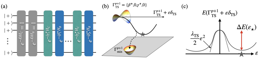
Figure 1: (a) Analytic construction of the particular transition state obtained from inserting two identity gates into QAOA_p circuit. (b) We inspect the energy alongside the unique descent direction associated with each of the transition states. The minimum along the unique descent direction (gray star marker) does not correspond to a stationary state of the energy. However, it lower bounds the energy of the minimum obtained by running optimization. (c) Sketch of the projected dependence of the cost function, with $\Delta E(\varepsilon_{*})$ putting a rigorous lower bound on the energy improvement at this iteration.

Finding the minimum of

$$E(\Gamma^{p})=\bra{\Gamma^{p}}H_{C}\ket{\Gamma^{p}}$$ (4)

over angles $(\beta_{1},\ldots,\beta_{p})$ and $(\gamma_{1},\ldots,\gamma_{p})$ that form a set of $2p$ variational parameters, $\Gamma^{p}=(\bm{\beta},\bm{\gamma})$, yields a desired approximation to the ground state of $H_{C}$, equivalent to an approximate a solution of MaxCut. The scalar function $E(\Gamma^{p})$ thus defines a $2p$-dimensional energy landscape where the global minimum yields the best set of QAOA parameters. The performance of the QAOA is typically reported in terms of how close is the approximation ratio to one,

$$1-r(\Gamma^{p})=\frac{E_{0}-E(\Gamma^{p})}{E_{0}},$$ (5)

where $E_{0}$ is the ground state of the classical Hamiltonian (1). From here we see that a decrease in $1-r$ implies that the expectation value of the cost function is approaching the ground state energy of the classical Hamiltonian.

Here, we restrict our attention to MaxCut on 3-regular graphs, where every vertex is connected to exactly 3 other vertices. In the main text, we focus on unweighted 3-regular graphs, while we delegate the results for weighted 3-regular graphs, with weights $J_{ij}$ chosen uniformly at random from the interval $[0,1]$, for the Appendix A. It is important to note that the results presented here are fully general (up to algebraic details), meaning that they hold for generic non-commuting Hamiltonians, $H_{C}$ and $H_{B}$, provided that the initial state $|\psi_{0}\rangle$ (or $|+\rangle$ in this work) is an eigenstate of $H_{B}$.

II.2 Analytical transition states

Most studies of the QAOA optimization landscape to date were restricted to local minima of the cost function $E(\bm{\beta},\bm{\gamma})$ since they can be directly obtained using standard gradient-based or some gradient-free optimization routines. Local minima are stationary points of the energy landscape, defined as $\partial_{i}E(\bm{\beta},\bm{\gamma})=0$, with the index $i$ ranging over all $2p$ variational parameters, where all eigenvalues of the Hessian matrix $H_{ij}=\partial_{i}\partial_{j}E(\bm{\beta},\bm{\gamma})$ are positive, that is the Hessian at the local minimum is positive-definite. The other stationary points with $0<k<2p$ negative Hessian eigenvalues are known as index-$k$ saddle points.

Work [26] analytically constructed index-$1$ saddle points dubbed transition states (TS) hereafter, of the QAOA_p+1 using a given local minimum of the QAOA_p, $\Gamma_{\min}^{p}$. This construction is illustrated in Fig. 1(a), and it consists of the insertion of a pair of identity gates, viewed as additional variational parameters initialized at a value equal to zero. Such insertion is allowed at $2p+1$ possible positions, giving rise to $2p+1$ distinct stationary points of the QAOA_p+1, $\Gamma_{\text{TS}}^{p+1}$ with a unique negative eigenvalue of the Hessian. We note that while showing that $\Gamma_{\text{TS}}^{p+1}$ constructed as above are stationary points is relatively straightforward, demonstrating that their Hessian has a single negative eigenvalue is less trivial, with a detailed proof available in Ref. [26].

Given that, by construction, all the $2p+1$ TS have the same energy as the initial local minimum $\Gamma^{p}_{\min}$, one can use the direction associated with the negative eigenvalue of the Hessian (hereafter referred to as index-1 direction) to further decrease the energy, see Fig. 1(b) for an example. In this way, the TS construction can be used as an initialization scheme that guarantees improvement of the QAOA performance with the circuit depth $p$ [26]. In this work, using the properties of the QAOA energy landscape in the vicinity of the transition states, we quantify the performance improvement of the QAOA by providing a lower bound for the energy improvement after an iteration of the QAOA.

III Curvature of energy landscape near transition state

In this section, we explore the curvature which is the first nontrivial local property of the QAOA energy landscape around the TS constructed out of a local minima $\Gamma^{p}_{\min}$ of the QAOA_p. Using the structure of the Hessian at the TS, we develop an approximation to its unique negative eigenvalue and its corresponding eigenvector. We also uncover connections between the negative curvature of the Hessian at the TS and the excited state population of the prepared QAOA state as a function of the circuit depth $p$.

III.1 Minimum Hessian eigenvalue and eigenvector

In this work, our analysis is specifically tailored to the scenario where additional identity gates are incorporated at the initial layer of the pre-existing QAOA_p circuit, as illustrated in Fig. 1(a). This particular scenario corresponds to the transition state denoted as $\Gamma_{\text{TS}}^{p+1}(1,1)$ in Ref. [26]. To maintain clarity and avoid unnecessary complexity in notation, we refer to this state more simply throughout our discussion when the context permits. We denote the transition state configuration as:

$$\Gamma_{\text{TS}}^{p+1}=(0,\beta_{1}^{\star},\ldots,\beta_{p}^{\star};0,\gamma_{1}^{\star},\ldots,\gamma_{p}^{\star}).$$ (6)

The primary reason for focusing on this specific transition state is that it significantly simplifies the analytical manipulations required for deriving the worst-case energy improvement achievable through optimizing QAOA_p+1, starting from a local minimum obtained by QAOA_p. Additionally, Appendix A presents numerical analyses that benchmark the effectiveness of this approach against the Greedy optimization strategy introduced on [26], which exploits all $2p+1$ transition states derived from $\Gamma^{p}_{\min}$.

In Appendix B, we first establish rigorous lower and upper bounds for the minimum Hessian eigenvalue. However, these bounds do not include an estimate for the corresponding Hessian eigenvector. To obtain this estimate, we construct a similarity transformation that transforms the Hessian at the transition state $\Gamma_{\text{TS}}^{p+1}$ into an almost block-diagonal form. By taking advantage of the Hessian structure, we derive a vector that refines the previously introduced upper bound for the minimum Hessian eigenvalue, which we then use as our estimate

$${\bm{\delta}}_{\text{TS}}=\left(-\frac{1}{2},\frac{1}{2},\underbrace{0,\ldots}_{p-1\leavevmode\nobreak\ \text{zeros}};-\frac{\operatorname{sign}(b)}{\sqrt{2}},\underbrace{0,\ldots}_{p\leavevmode\nobreak\ \text{zeros}}\right),$$ (7)

where the parameter $b$ is the second derivative of the cost function $b=\partial_{\gamma_{1}}\partial_{\beta_{1}}E(\Gamma^{p+1}_{\mathrm{TS}})$, which can be expressed as a nested commutator of the following three operators:

$$b=\langle+|[H_{C},[H_{B},U^{\dagger}(\Gamma^{p}_{\min})H_{C}U(\Gamma^{p}_{\min})]]|+\rangle.$$ (8)

The approximate form of the eigenvector (7) shows that when initialized from the former minima of QAOA_p, the classical optimization procedure changes values of angles $\beta_{1}$, $\gamma_{1}$ that were initialized at zero initially, as well as the value of $\beta_{2}=\beta_{1}^{\star}$ initialized at the value set by the local minimum at depth $p$. All remaining parameters are left intact at the start of gradient descent. The expression for $b$ above can be further simplified relying on the specific expressions for $H_{C}$ and $H_{B}$, using Eq. (1) and Eq. (3) respectively

$$b=8\langle+|H_{C}U^{\dagger}(\Gamma^{p}_{\min})H_{C}U(\Gamma^{p}_{\min})|+\rangle.$$ (9)

Finally, we approximate the minimum Hessian eigenvalue $\lambda_{\mathrm{TS}}$ by the expectation value of the Hessian on the approximate eigenvector $\bm{\delta}_{\mathrm{TS}}$, obtaining that it is proportional to the second derivative $b=\partial_{\gamma_{1}}\partial_{\beta_{1}}E(\Gamma^{p+1}_{\mathrm{TS}})$ defined above:

$$\lambda_{\mathrm{TS}}=-\frac{|b|}{\sqrt{2}}=-4\sqrt{2}|\langle+|H_{C}U^{\dagger}(\Gamma^{p}_{\min})H_{C}U(\Gamma^{p}_{\min})|+\rangle|.$$ (10)

We refer the discussion of the physical intuition behind this expression to the Sec. III.3, where we show that $\lambda_{\mathrm{TS}}$ vanishes in the case when QAOA unitary circuit rotates the $|+\rangle$ state into an exact eigenstate of $H_{C}$. It is critical to note that our estimation of the minimum Hessian eigenvalue is potentially computable on a NISQ device. From the form of the transition state specified by Eq. (6), we deduce that the value of $b$ in Eq. (9) can be estimated on a NISQ device using additionally $\mathcal{O}(n_{\mathcal{E}}(\mathcal{G}))$ more circuit executions. Here, $n_{\mathcal{E}}(\mathcal{G})$ denotes the number of edges (interaction terms) in the problem graph $\mathcal{G}$ that determines the cost Hamiltonian Eq. (1).

Although in this Section we focused on the transition state obtained by padding with zeros the first layer of the QAOA, in the Appendix B, we show that a similar approach allows us to obtain estimates of eigenvectors and eigenvalues for all the $2p+1$ TS. For a generic transition state $\Gamma^{p+1}_{\mathrm{TS}}(i,j)$, the approximate Hessian eigenvector has non-zero components corresponding to adjacent gates, that is $\beta_{i},\beta_{i+1},\gamma_{j}$, and $\gamma_{j-1}$. Moreover, the approximate eigenvalue is given by a particular matrix element of the Hessian when the zeros insertion is at the first or last layer, or by a difference of two particular matrix elements in the Hessian matrix for all remaining transition states. In all the cases, our approximation to the eigenvalue is a measurable quantity, which can be estimated analogously to the procedure described after Eq. (10).

III.2 Quality of the curvature approximation

To assess the accuracy of our estimates for the true minimum Hessian eigenvalue and its corresponding eigenvector, we examine a collection of non-isomorphic random instances of 3-regular unweighted graphs with $N=10,\ldots,16$ vertices—18, 34, 55, and 40 instances respectively—executing the QAOA for circuit depths within the range $p\in[1,30]$. For each local minimum obtained at a given circuit depth $p$, we construct the $2p+1$ transition states and compute their exact numerical Hessians. After determining the Hessian spectrum, we calculate the relative error of our minimum eigenvalue estimate and the deviation of the absolute overlap between the approximate and exact Hessian eigenvector from 1.

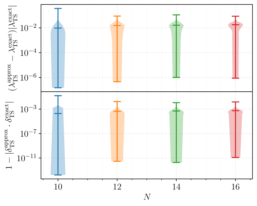
Figure 2: Accuracy of curvature and descent direction estimates shown by violin plots for QAOA transition states across graph instances with 10 to 16 vertices and circuit depths ranging from 1 to 30. (Top) Relative error in the negative Hessian eigenvalue estimation; the median error is indicated by the horizontal line. (Bottom) Deviation from unity in the absolute overlap between the estimated and exact eigenvectors associated with the negative eigenvalue. The shaded regions capture the probability density of the data, reflecting that the accuracy of our eigenvector estimate is consistent across different system sizes.

We consolidate our findings in Fig. 2, which is composed of “violin plots” that illustrate the distribution of the obtained numerical data. The width of each violin indicates the frequency of data points at different error or overlap values, providing insight into the variability of the measures. Typically, the median of the data—indicated by the horizontal line within each violin—reveals that the relative error in the minimum Hessian eigenvalue is on the order of $O(10^{-2})$, while the deviation from 1 of the absolute value of the overlap between the exact and approximate eigenstates is on the order of $O(10^{-3})$. More critically, the shape and extent of the violins suggest that the accuracy of our estimates remains consistent across all system sizes and instances examined. This visual analysis underlines the reliability of the estimates provided by our method, with the precision of our estimate appearing stable upon increasing the number of qubits $N$.

III.3 Evolution of the curvature with the depth of QAOA

In this section, we focus on the behavior of the curvature with the circuit depth $p$. First, we demonstrate that $\lambda_{\mathrm{TS}}$ is vanishing when QAOA_p prepares an eigenstate of the cost Hamiltonian $H_{C}$, thereby being proportional to the square root of the infidelity of the eigenstate preparation. Moreover, we build a physical intuition for the value of curvature by relating it to the action of QAOA circuit on the excited states of the mixing Hamiltonian. Next, we suggest the parallel in the behavior of the curvature and the energy variance of the state prepared in the QAOA circuit with respect to the cost Hamiltonian. Finally, we test our arguments numerically, demonstrating that similarly to the $1-r$, where $r$ is the QAOA approximation ratio, vanishing exponentially with the circuit depth $p$, the curvature and energy variance also decrease exponentially.

To provide the physical intuition for the value of $\lambda_{\mathrm{TS}}$ in Eq. (10), we write quantum states $U(\Gamma^{p}_{\min})|+\rangle$ and $U(\Gamma^{p}_{\min})H_{C}|+\rangle$ in the following form

$$\begin{split}U(\Gamma^{p}_{\min})|+\rangle&=\alpha^{0}|E_{0}\rangle+\alpha^{0}_{\perp}|\psi_{0}\rangle,\\ U(\Gamma^{p}_{\min})H_{C}|+\rangle&=n_{C}\kappa^{0}|E_{0}\rangle+n_{C}\kappa^{0}_{\perp}|\phi_{0}\rangle,\end{split}$$ (11)

where we have selected out the ground state of the classical Hamiltonian, $|E_{l=0}\rangle$ (this can be any eigenstate of $H_{C}$, not necessarily the ground state, as we will discuss later), and remaining states $|\psi_{0}\rangle$ and $|\phi_{0}\rangle$ in this expansion are normalized superposition of all other eigenstates of $H_{C}$, thus being orthogonal to $|E_{0}\rangle$ by construction. The constant $n_{C}=\sum_{\langle ij\rangle}J^{2}_{ij}$ comes from the norm of $H_{C}|+\rangle$ and it is added such that $|\kappa^{0}|^{2}+|\kappa^{0}_{\perp}|^{2}=1$.

Notations introduced in Eq. (11) allow us to rewrite the expression for the curvature, Eq. (10), as

$$|\lambda_{\mathrm{TS}}|=4\sqrt{2}n_{C}\alpha^{0}_{\perp}\kappa^{0}_{\perp}|\langle\phi_{0}|H_{C}-E_{0}|\psi_{0}\rangle|,$$ (12)

where without loss of generality we assume that factors in this expression, $\alpha^{0}_{\perp}$ and $\kappa^{0}_{\perp}$, are real positive numbers. In notations of Eq. (11) $\alpha^{0}$ corresponds to the square root of the fidelity of the QAOA prepared state $U(\Gamma^{p}_{\min})|+\rangle$ to the ground state $|E_{0}\rangle$ of $H_{C}$ with eigenvalue $E_{0}$, and $\alpha^{0}_{\perp}=\sqrt{1-|\alpha^{0}|^{2}}$ is the infidelity. Crucially, the second line of Eq. (11) defines $\kappa^{0}$ as square root of the fidelity between states $|E_{0}\rangle$ and $U(\Gamma^{p}_{\min})H_{C}|+\rangle$, where the latter state physically corresponds to the QAOA circuit applied to an excited eigenstate of the mixing Hamiltonian with eigenvalue $-N+4$ (for more general forms of $H_{C}$ and $H_{B}$, we expect this state to be a combination of low-lying excited eigenstates of $H_{B}$). Since the curvature $\lambda_{\mathrm{TS}}$ is proportional to the product of $\alpha^{0}_{\perp}$ and $\kappa^{0}_{\perp}$, it implies that it is sensitive not only to the infidelity resulting from the QAOA circuit preparing the desired ground state of the cost Hamiltonian, but also to the behavior of the low-lying excited state of the mixing Hamiltonian as it is acted upon by the QAOA circuit.

From expression (12), we realize that a non-zero curvature around the transition state $\Gamma^{p+1}_{\mathrm{TS}}$ comes from the fact that the QAOA circuit prepares a superposition of energy eigenstates as quantified by $\alpha^{0}_{\perp}\neq 0$ and $\kappa^{0}_{\perp}\neq 0$. Furthermore, to determine the curvature we need information on what superposition of eigenstates of the classical Hamiltonian the QAOA unitary creates when acting on the superposition of states $\sigma^{z}_{i}\sigma^{z}_{j}|+\rangle$, with $\langle i,j\rangle\in\mathcal{E}_{G}$ corresponding to an edge in the problem graph $G$, that are the superposition of second excited states (two spin flips in $x$ basis) of the mixing Hamiltonian.

Finally, we did not discuss the role of the expectation value, $\langle\phi_{0}|H_{C}-E_{0}|\psi_{0}\rangle$ in Eq. (12). On the one hand, this matrix element is expected to be extensive, i.e. increasing proportionally to number of degrees of freedom, $N$, as is also confirmed by our numerical simulations, see Figs. 3 and 10. On the other hand, estimating the scaling of this matrix element with $p$ remains an open challenge. The contributions to this expectation value primarily arise from eigenstates of $H_{C}$ where both $|\phi_{0}\rangle$ and $|\psi_{0}\rangle$ have significant weight. Developing a framework to accurately assess these contributions and their scaling with $p$ based on physically motivated assumptions remains an intriguing open problem.

Another physical quantity that quantifies the deviation of the state $|\Gamma^{p}_{\text{min}}\rangle$ from an eigenstate of the cost Hamiltonian $H_{C}$ is the energy variance. Using the notation of Eq. (11) we express the energy variance as

$$\mathrm{var}_{|\Gamma^{p}_{\min}\rangle}[H_{C}]=\langle\Gamma^{p}_{\min}|H^{2}_{C}|\Gamma^{p}_{\min}\rangle-\langle\Gamma^{p}_{\min}|H_{C}|\Gamma^{p}_{\min}\rangle^{2},$$

$$=|\alpha^{0}_{\perp}|^{2}\mathrm{var}_{|\psi_{0}\rangle}[H_{C}]+|\alpha^{0}_{\perp}|^{2}|\alpha^{0}|^{2}(\langle\psi_{0}|H_{C}|\psi_{0}\rangle-E_{0})^{2}.$$ (13)

From this expression, it is apparent that the energy variance is proportional to the same infidelity of the state $U(\Gamma^{p}_{\min})|+\rangle$ to the ground state.

Comparing expressions (12)-(III.3), we expect both $|\lambda_{\rm{TS}}|$ and energy variance to display similar qualitative behavior with the circuit depth $p$. Thus, we establish a connection between two seemingly unrelated properties: the energy variance of the quantum state prepared by the QAOA_p circuit and the curvature of the cost function of the QAOA_p+1 at the transition state. Since so far we focused on the ground state $|E_{0}\rangle$ of $H_{C}$, and previous literature [23, 22] heuristically demonstrated that for the MaxCut problem on unweighted 3-regular graphs, the approximation ratio $r(\Gamma)$ tends towards 1 exponentially with increasing circuit depth $p$, we anticipate that infidelity $\alpha^{0}_{\perp}$ also tends to zero exponentially, thus leading to an exponential decrease in both curvature and energy variance to zero.

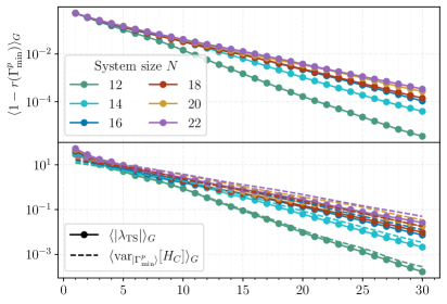
Figure 3: (Top) Circuit depth dependence of the approximation ratio $r(\Gamma^{p}_{\min})$, which approach zero exponentially with $p$. These results were initially observed in [22, 23]. (Bottom) Relation between the magnitude of the negative curvature around the transition state $\Gamma^{p+1}_{\mathrm{TS}}$, and the energy variance $\mathrm{var}_{\Gamma^{p}_{\min}}[H_{C}]$ as functions of the circuit depth $p$. The numerical data reveals a notable quantitative alignment between the curvature and the energy variance for varying system sizes $N$.

To validate our expectations, we first reproduced the numerically observed exponential convergence of QAOA. We then calculated the average absolute value of $\lambda_{\mathrm{TS}}$ across various unweighted MaxCut instances with $N$ ranging from 12 to 22 vertices. The obtained results are displayed in Fig. 3 together with the average of the approximation ratio for circuit depths ranging in the interval $p\in[1,30]$. The top panel of this figure reproduces the exponential decrease of $1-r$ with circuit depth $p$ [22, 23]. The bottom panel shows the surprisingly close quantitative agreement between the averaged energy variance and the absolute value of the negative curvature $|\lambda_{\mathrm{TS}}|$. This signals that these quantities can be related in a tighter way than what we discussed above, in particular, the constants $\alpha^{0}_{\perp}$ and $\kappa^{0}_{\perp}$ may be proportional to each other.

Finally, we want to highlight some possible implications of the above observations for the performance of the QAOA at finite but deep circuit depth. First, our results above imply that if the QAOA prepares an eigenstate $|E_{l}\rangle$ that is different from the ground state, $l>0$, of the cost Hamiltonian $H_{C}$ the optimization strategy that uses transition states as initialization will halt since there are no descent directions around any of the transition states. Assuming that the ground state is challenging to prepare for whatever reason, it may be feasible for the QAOA to instead prepare a low-lying eigenstate $|E_{l}\rangle$ with $l>0$ but not too large, with high fidelity ($|\alpha^{l}|\sim 1$). As a consequence, the local negative curvature around each TS will become small and as a result, we expect the optimization to slow down. In Appendix A, we illustrate this scenario in an instance of a weighted 3-regular graph that was originally studied in [23].

Thus, our results that relate the landscape curvature at the TS, the energy variance of the QAOA state, and infidelity, suggest that using the Greedy strategy (or similarly using the TS $\Gamma^{p+1}_{\mathrm{TS}}(1,1)$) the QAOA may effectively converge to a (low) energy manifold of the cost Hamiltonian $H_{C}$ in the regime of deep circuit. Quantifying how this convergence happens remains an open problem, but in the next section we make the first steps in this direction by expanding the cost function to higher order around the transition state.

IV Higher order expansion of energy along index-1 direction

In this section we use the approximate index-1 direction given by Eq. (7) to expand the QAOA_p+1 cost function up to the fourth order along the descent direction. This results in lower bound on the improvement of the QAOA cost function resulting from increasing the number of parameters from $2p$ to $2p+2$.

IV.1 Taylor expansion

Using the explicit knowledge of the index-1 descent direction, we estimate how much the energy can be improved using the Taylor series expansion around the point $\Gamma_{\mathrm{TS}}^{p+1}$. Specifically, Appendix C details our computation of the cost function’s expansion, $E(\Gamma_{\mathrm{TS}}^{p+1}+\varepsilon{\bm{\delta}}_{\mathrm{TS}})$, to the fourth order in $\varepsilon$. In what follows, we neglect the cubic term in the energy expansion, delegating the details of such step to the Appendix C, and obtain a simple expression:

$$E(\Gamma_{\text{TS}}^{p+1}+\varepsilon{\bm{\delta}}_{\text{TS}})\approx E(\Gamma^{p}_{\text{min}})+\frac{\lambda_{\rm{TS}}}{2}\varepsilon^{2}+\partial_{\gamma_{1}}^{2}E(\Gamma^{p+1}_{\text{TS}})\varepsilon^{4},$$ (14)

where $\partial_{\gamma_{1}}^{2}E(\Gamma^{p+1}_{\text{TS}})$ is expressed as a combination of two expectation values:

$$\partial^{2}_{\gamma_{1}}E(\Gamma^{p+1}_{\rm{TS}})=2\langle+|H_{C}U(\Gamma^{p}_{\text{min}})^{\dagger}H_{C}U(\Gamma^{p}_{\text{min}})H_{C}|+\rangle\\ -2\Re{\langle+|U(\Gamma^{p}_{\text{min}})^{\dagger}H_{C}U(\Gamma^{p}_{\text{min}})H_{C}^{2}|+\rangle}.$$ (15)

The fact that the fourth order expansion term of energy is proportional to the second derivative, $\partial^{2}_{\gamma_{1}}E(\Gamma^{p+1}_{\rm{TS}})$ can be understood from the specific form of the descent direction vector, Eq. (6). Using the explicit form of the descent vector, in Appendix C we show that the first non-trivial expansion term in $\varepsilon$ of the state $U(\Gamma^{p+1}_{\text{TS}}+\varepsilon{\bm{\delta}}_{\text{TS}})\ket{+}$ is proportional to $\varepsilon^{2}H_{C}\ket{+}$. Combining two of such terms, we precisely get the contribution in the first line of Eq. (15) above, which is thus coming with an order of $\varepsilon^{4}$.

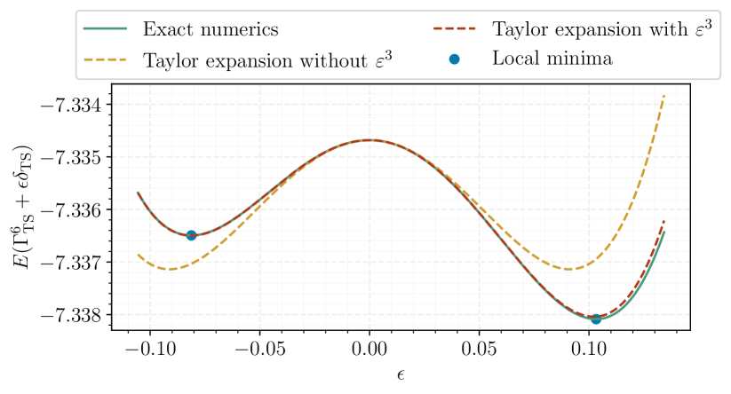
Figure 4: Taylor approximation of the energy at a transition state obtained from a local minima of QAOA₅ when perturbed in the index-1 direction. We inspect the impact of the cubic term in the perturbation parameter $\varepsilon$ in the energy expansion around the index-1 direction. The instance studied corresponds to that of Appendix A.

In Fig. 4, we assess the Taylor approximation’s accuracy (which incorporates a cubic term in $\varepsilon$) against exact numerical data obtained by computing the Hessian at $\Gamma^{p+1}_{\mathrm{TS}}$ and determining the energy along the exact index-1 direction. Additionally, we examine the impact of omitting the cubic term from the expansion. While the omission of the cubic term leads to underestimation of the energy improvement, it significantly streamlines the energy expansion analysis and still faithfully replicates the qualitative behavior of exact energy depenence on the slice.

IV.2 Comparing estimated and true energy gains

Using the expression for the energy Eq. (14) along the index-1 direction we compute the value of the perturbation parameter $\varepsilon$ that minimizes the energy in this univariate optimization problem. The solution then reads

$$\Delta E(\varepsilon_{*})=E(\Gamma^{p+1}_{\text{TS}}+\varepsilon_{*}\delta_{\text{TS}})-E(\Gamma^{p}_{\min})\\ =-\frac{\lambda_{\mathrm{TS}}^{2}}{16\partial^{2}_{\gamma_{1}}E(\Gamma^{p+1}_{\mathrm{TS}})},$$ (16)

with the distance from the transition state to the local minimum on the slice corresponding to $\varepsilon^{2}_{*}=-\lambda_{\mathrm{TS}}/4\partial^{2}_{\gamma_{1}}E(\Gamma^{p+1}_{\mathrm{TS}})$. We note that although from the expansion of the cost function we get the local energy minimum, this is the artifact of the considering only one out of $2p+2$ directions in the energy landscape. When viewed without projection, we do not expect the point $\Gamma^{p+1}_{\text{TS}}+\varepsilon_{*}\delta_{\text{TS}}$ to be a local minimum or even a saddle point of the cost function, see Fig. 1(b).

Using the expression for $\lambda_{\text{TS}}$ obtained in the previous section in Eq. (12) we see that the numerator in Eq. (16) is proportional to the square root of the infidelity $\alpha^{0}_{\perp}$ to the ground state $|E_{0}\rangle$. Furthermore, we expect that $\partial^{2}_{\gamma_{1}}E(\Gamma^{p+1}_{\mathrm{TS}})$ in the denominator remains finite and extensive in the deep QAOA limit. In particular, in Appendix C we discuss that $\partial^{2}_{\gamma_{1}}E(\Gamma^{p+1}_{\mathrm{TS}})$ can be approximated as follows:

$$\partial^{2}_{\gamma_{1}}E(\Gamma^{p+1}_{\mathrm{TS}}) \approx 2n_{C}^{2}\langle+|\frac{H_{C}}{n_{C}}U^{\dagger}(\Gamma^{p}_{\min})H_{C}U(\Gamma^{p}_{\min})\frac{H_{C}}{n_{C}}|+\rangle$$

$$-2n_{C}^{2}E(\Gamma^{p}_{\min}).$$ (17)

where for clarity we explicitly singled out the common factor of $n_{C}$ that highlights the scaling of quartic expansion coefficient. From Eq. (IV.2) the quartic coefficient in the expansion of energy, $\partial^{2}_{\gamma_{1}}E(\Gamma^{p+1}_{\mathrm{TS}})$, can be understood as the energy difference between states $U(\Gamma^{p}_{\min})H_{C}|+\rangle$ and $U(\Gamma^{p}_{\min})|+\rangle$, multiplied by the extensive constant $n_{C}^{2}\sim N$. It is natural to expect that QAOA circuit, when applied to the excited eigenstate of the mixing Hamiltonian, $H_{C}|+\rangle$, yields the final state that has higher energy compared to the state $U(\Gamma^{p}_{\min})|+\rangle$, that QAOA circuit by design aims to rotate into the ground state of classical Hamiltonian. This physical reasoning implies that the quartic expansion coefficient, $\partial^{2}_{\gamma_{1}}E(\Gamma^{p+1}_{\mathrm{TS}})$, is positive, as is also confirmed in numerical simulations. As the algorithm converges at large enough circuit depths $p$, we expect $\partial^{2}_{\gamma_{1}}E(\Gamma^{p+1}_{\mathrm{TS}})$ to plateau at an extensive value. Finally, it is important to note that the $n_{C}^{2}$ factor in the denominator of Eq. (16) cancels out with the same factor coming from $|\lambda_{\mathrm{TS}}|\propto n_{C}$, see Eq. (12).

We use numerical simulations to verify the validity of the approximation given by Eq. (IV.2), on random instances of unweighted 3-regular graphs with $N=[12,22]$ vertices. From Fig. 5, we observe a clear extensive behavior of $\partial^{2}_{\gamma_{1}}E(\Gamma^{p+1}_{\mathrm{TS}})$. Interestingly, we see that even though the data for different system sizes does not perfectly collapse onto a single curve, its dependence on the system size at all circuit depths is relatively weak. For example, at $p=30$ the values for different systems sizes lie in the interval $[11,13]$.

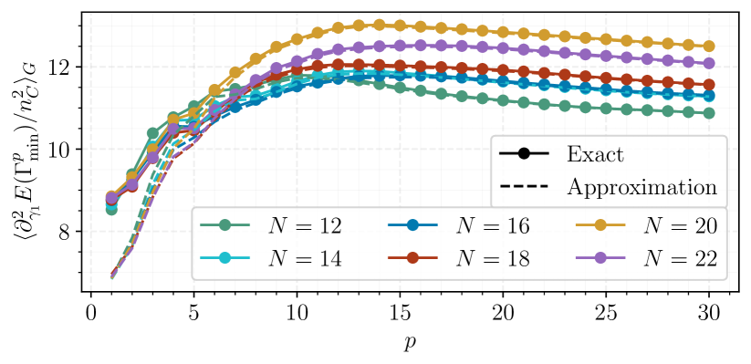
Figure 5: Averaged circuit depth behavior of $\partial^{2}_{\gamma_{1}}E(\Gamma^{p+1}_{\mathrm{TS}})$ and its approximation Eq. (IV.2) for different system sizes agree for $p\geq 5$.

Using the intuition that the quartic term that represents the denominator in the expression for energy gain, Eq. (16) is saturating to the finite value for large $p$, we conclude that the lower bound on the energy gain is proportional to the curvature around the transition state, and thus is expected to decrease exponentially with the circuit depth $p$, as supported by the analysis in the previous section. We numerically check the tightness of the lower bound provided by Eq. (16).

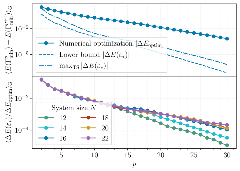
Figure 6: (Top) Average energy improvement between local minima of QAOA_p and QAOA_p+1 as a function of the circuit depth $p$ for an unweighted 3-regular graph with $N=16$ vertices. The lower bound Eq. (16), which relies on local information about the cost function landscape around index-1 saddle points overestimates the results obtained by numerically optimizing using the Greedy strategy of [26]. (Bottom) Averaged quality of the lower bound on the energy improvement, as given by $\Delta E(\varepsilon_{*})/\Delta E_{\mathrm{optim}}$, for systems sizes ranging from 12 to 22 vertices.

To this end, in Fig. 6 we first take random instances of unweighted 3-regular graphs with $N=16$ vertices and compare Eq. (16) to the energy improvement coming from performing numerical optimization, using the Broyden–Fletcher–Goldfarb–Shanno (BFGS) algorithm [28, 29, 30, 31], following the Greedy strategy introduced in [26]. We also show the best improvement selected from improvements obtained from moving along the index-1 direction of $2p+1$ distinct TS obtained from the initial local minima $\Gamma^{p}_{\min}$, labeled as $\max_{\text{TS}}[\Delta E(\varepsilon_{*})]=\max_{(i,j)}\big{[}E(\Gamma^{p}_{\min})-E(\Gamma^{p+1}_{\mathrm{TS}}(i,j)+\varepsilon\delta_{\mathrm{TS}})\big{]}$.

Figure 6 reveals that the true energy improvement, and our lower bound Eq. (16) both decrease exponentially with $p$, although with different slopes. In particular, the energy improvement from moving alongside the index-1 direction underestimates the improvement obtained from numerical optimization. This allows us to conclude that although the BFGS optimization algorithm using a large number of iterations can find better local minima by moving far away from the transition state, the entire cost function landscape is getting more “flat” with $p$. Thus, while our lower bound, which is conceptually similar to one step of local optimization, is underestimating the magnitude of the energy improvement, it has the same functional dependence on $p$. It remains to be understood if one can establish a (heuristic) relation between our bound and the true energy decrease, thus allowing us to predict the QAOA performance quantitatively from Eq. (16).

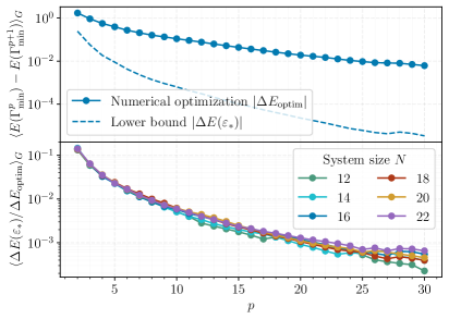
Figure 11: (Top) Average energy improvement between local minima of QAOA_p and QAOA_p+1 as a function of the circuit depth $p$. The lower bound Eq. (16), which relies on local information about the cost function landscape around index-1 saddle points overestimates the results obtained by numerically optimizing using the Greedy strategy of [26]. (Bottom) Averaged quality of the lower bound on the energy improvement, as given by $\Delta E(\varepsilon_{*})/\Delta E_{\mathrm{optim}}$, for systems sizes ranging from 12 to 22 vertices.

Finally, we discuss the scaling of energy improvement with system size, as shown in the bottom panel of Fig. 6. Similar scaling is also evident in instances of MaxCut on 3-regular weighted graphs, as illustrated in Fig. 11 in Appendix A. The numerical results show that at a fixed circuit depth our bound on energy improvement is proportional to the system size $N$. Indeed, we show that the ratio between the numerical energy improvement and our estimate tends to a constant value with increasing system size, and numerical energy improvement is known to be proportional to $N$. Analytically, this behavior arises from the expectation value $|\langle\phi_{0}|H_{C}-E_{0}|\psi_{0}\rangle|$ in the expression for the approximate negative Hessian eigenvalue in Eq. (12) which is extensive in $N$. In summary, the scaling of our bound on energy improvement with $N$ implies that the improvement in approximation ratio does not scale with $N$, which is consistent with the gains from numerical optimization.

V Discussion

In this work, we perform an analytic study of transition states of the QAOA cost function, that were constructed in Ref. [26]. These transition states are characterized by the vanishing gradient of the cost function and a unique negative eigenvalue of Hessian. In the present work, we provide an accurate analytic estimate of the minimum eigenvalue of the Hessian and its corresponding eigenvector for each of the $2p+1$ TS. Moreover, we relate the curvature in the vicinity of transition states to physical observables such as the infidelity of the ground state preparation of the QAOA circuit, and construct the higher-order expansion of the QAOA cost function along the negative curvature direction, which allows us to put a lower bound on the QAOA cost function improvement.

Crucially, the results obtained in this paper are recursive. Assuming that QAOA at depth $p$ found a local minimum, we provide a lower bound on the cost function improvement of the QAOA at depth $p+1$. Thus, our approach is applicable to QAOA in the regime of large $p$ and we envision that it may be potentially used to obtain a QAOA performance guarantee [4, 11, 7]. Indeed, the only missing link in such performance guarantee remains to be the bound on the improvement in infidelity, which determines the landscape curvature and lower-bounds energy improvement as shown by our work.

Beyond being a potential step towards performance guarantee, the significance of these estimates is twofold: first, they substantially reduce the computational effort required to implement the Greedy optimization strategy outlined by [26], as they circumvent the need to construct and diagonalize the Hessian of the cost function at each TS. Second, our results establish the analytical framework that reveals properties of the QAOA cost function at arbitrarily large $p$.

In particular, we show that for unweighted 3-regular graphs, the negative curvature of the landscape at the TS is intimately connected to the energy variance of the QAOA state. This not only offers a physical interpretation of the negative curvature at the TS but also raises questions about the QAOA performance in the limit of large circuit depth. While it is anticipated that the QAOA will prepare the ground state as $p\to\infty$ [4], our findings suggest that the QAOA may effectively converge to a (low) energy manifold of the cost Hamiltonian $H_{C}$ in the deep circuit regime.

Furthermore, our numerical analyses indicate that the lower bound on the energy improvement has the same qualitative dependence on the QAOA depth as the true energy improvement. At the same time, our lower bound parametrically underestimates the actual improvements achieved through numerical optimization. This observation suggests that the local vicinity of the transition state that we can explore analytically may be non-trivially related to the global properties of the QAOA cost function. Establishing such a relation even heuristically may be useful for accurately forecasting the performance of the QAOA, and may provide a useful step towards a more complete understanding of the QAOA.

Finally, given the broad applicability of the transition states-based approach, it becomes intriguing to consider its extension to problems beyond the MaxCut. Exploring the impact of different cost and mixer Hamiltonians on the QAOA cost function landscape presents a promising avenue for future research. Additionally, applying the transition state (TS) strategy to other variational algorithms offers an exciting opportunity. By leveraging the unique characteristics of both the circuit and the problem structure, it may be possible to provide similar initialization strategies and devise analytic estimates for the improvement of the cost function from the optimization process.

Appendix A Numerical simulations

In this appendix, we first introduce the package used for numerical simulations throughout this work. Next, we justify the choice of the first transition state as a focus of the main paper. For this, we demonstrate that considering only the first transition state, defined in Eq. (6), does not degrade the initialization performance compared to the case when one uses $2p+1$ TS. Next, we discuss and show how the QAOA can converge to an excited state of the cost Hamiltonian $H_{C}$ for a wide range of circuit depths $p$, and how this is reflected in the non-monotonic behavior of the landscape curvature at the transition state. Finally, we conclude this appendix by discussing numerical results for weighted instances of MaxCut on 3-regular graphs.

A.1 Package QAOALandscapes.jl for numerical simulations of QAOA in Julia

All the simulations performed in this work were conducted using the Julia programming language [32] and the package QAOALandscapes.jl[33], which was developed by one of the authors. This package is designed to apply the QAOA to solve general combinatorial optimization problems by encoding the classical problem into a $k$-spin classical Hamiltonian. It relies on matrix-free operations to enhance speed and reduce memory usage. Currently, it supports only the Pauli-$X$ mixer operator (see Eq.(3)); however, additional mixers can be incorporated as is described in the documentation. The package includes support for both CPU and GPU backends, with GPU capabilities for CUDA and Metal-based devices through CUDA.jl [34, 35] and Metal.jl [36] packages respectively.

Numerical optimization was performed using the Optim.jl [37, 38] package, and in particular using the BFGS [28, 29, 30, 31] algorithm. For this, the package supports fast and exact gradient calculations through the use of automatic differentiation using the method introduced in [39, 40]. Further details on how to use QAOALandscapes.jl can be found on the Readme and documentation in [33].

A.2 Quality of optimization using only $\Gamma^{p+1}_{\mathrm{TS}}(1,1)$

The Greedy approach introduced in [26], requires one to launch optimization twice from each of the $2p+1$ TS constructed from a local minimum $\Gamma^{p}_{\min}$ of QAOA_p. The need to launch optimization from $2p+1$ distinct transition states and moving in two potential directions away from the saddle accounts for a $2(2p+1)$ overhead on top of heuristic initializations like Interp and Fourier [23] with similar performance. Even though Greedy comes with a guarantee of improvement at each circuit depth $p$, it is desirable to further reduce the optimization cost that it incurs.

We thus inspect given a local minimum $\Gamma^{p}_{\min}$ what fraction of the $2p+1$ TS constructed from it leads to the Greedy solution after optimization. We numerically observe in Fig. 7 that the number of TS that connect through optimization to the best local solution decreases with $p$ but remains finite at approximately 0.7 at circuit depth $p=20$. In all cases, we observed that the transition state constructed by padding with zeros the first layers, i.e. $\Gamma^{p}_{\mathrm{TS}}(1,1)$ in the notation of [26], leads to the Greedy solution as also shown in the figure, where we plot the average approximation ratio obtained from using the Greedy strategy, and the result coming from only using $\Gamma^{p}_{\mathrm{TS}}(1,1)$.

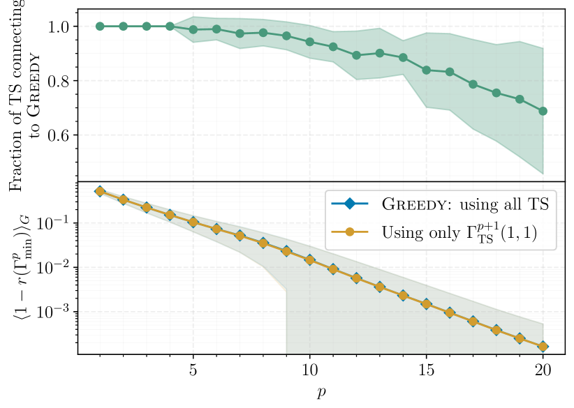
Figure 7: (Top) Fraction of the $2p+1$ TS constructed from a local minima $\Gamma^{p}_{\min}$ that connect to the Greedy solution. The data corresponds to instances of random 3-regular unweighted graphs with $N=12$ vertices. (Bottom) Performance of numerical optimization using only the transition state with zeros padded at indices $(\beta,\gamma)=(1,1)$. The average performance, over instances of 3-regular unweighted graphs with $N=12$ vertices seems effectively identical to that of the Greedy strategy [26] that uses the set of all $2p+1$ TS constructed from a local minima of QAOA_p.

This observation motivates us to focus on the transition state $\Gamma^{p}_{\mathrm{TS}}(1,1)$ as it provides a reliable choice of an initial transition state. Fixing the transition state in such a way reduces the cost of optimization to a simple factor of two, while still keeping the guarantee of improvement. Furthermore, as we will show below, using $\Gamma^{p}_{\mathrm{TS}}(1,1)$ enables us to obtain a lower bound on the energy improvement of the QAOA between circuit consecutive circuit depths.

A.3 Converging to an excited state

Here we provide a specific example of QAOA converging to an excited state. To this end, we use a MaxCut instance studied in Ref. [23]. This instance was used to highlight the performance of the Fourier and Interp strategies [23] on “hard” instances of MaxCut. The authors used the minimum spectral gap $\Delta_{\min}$ of the annealing Hamiltonian

$$H_{\mathrm{QA}}(s)=sH_{C}+(1-s)H_{B};\;s\in[0,1]$$

to distinguish between “hard” and “easy” instances for optimization. In particular, for the instance shown in Fig. 8 one can show that $\Delta_{\min}<10^{-3}$, which translates into prohibitively long annealing time [23].

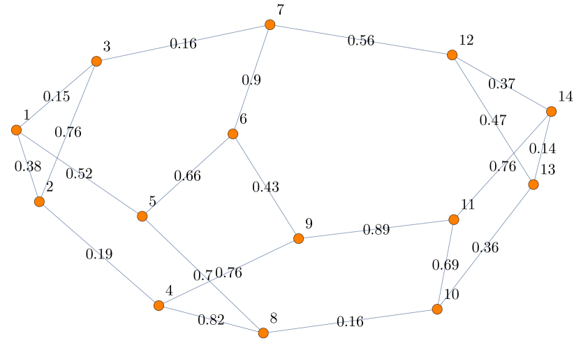
Figure 8: Instance of MaxCut with $N=14$ vertices where the QAOA algorithm gets trapped in local optima, and mostly converges to the first excited state of the cost Hamiltonian $H_{C}$.

Both Fourier and Interp initialization strategies reuse a local minimum of the QAOA at circuit depth $p$ to construct an initialization at circuit depth $p+1$. In the case of the Fourier initialization — which will also use here — the idea is to use a different parametrization of QAOA. Instead of using the $2p$-parameters $(\bm{\beta},\bm{\gamma})$, Ref. [23] considers the discrete cosine and sine transform of $\bm{\beta}$ and $\bm{\gamma}$ respectively

$$\beta_{i} =\sum_{k=1}^{q}v_{k}\cos[(k-\frac{1}{2})(i-\frac{1}{2})\frac{\pi}{p}\big{]},$$ (18)

$$\gamma_{i} =\sum_{k=1}^{q}v_{k}\sin[(k-\frac{1}{2})(i-\frac{1}{2})\frac{\pi}{p}\big{]}.$$ (19)

Through such coordinate transformation, the new parameters become the amplitudes $(\bm{v},\bm{u})$ of the frequency components for $\bm{\beta}$ and $\bm{\gamma}$, respectively. The basic Fourier$[\infty,0]$ variant of the strategy, generates a good initial point for QAOA_p+1 by adding a higher frequency component, initialized at zero amplitude, to the optimum at level $p$. Last, in the improved variant Fourier$[\infty,R]$ in addition to optimizing according to the basic strategy, we optimize QAOA_p+1 from $R+1$ extra initial points, $R$ of which are generated by adding random perturbations to the best of all local optima $(\bm{v},\bm{u})$ found at level $p$ (see the Appendix B.2 in Ref. [23] for more details). It is crucial to note that the number of random perturbations in Fourier space, denoted by $R$, serves as a hyperparameter; optimizing its value is essential for enhanced convergence, requiring multiple runs of the optimization process with varied $R$ settings to determine the most effective configuration.

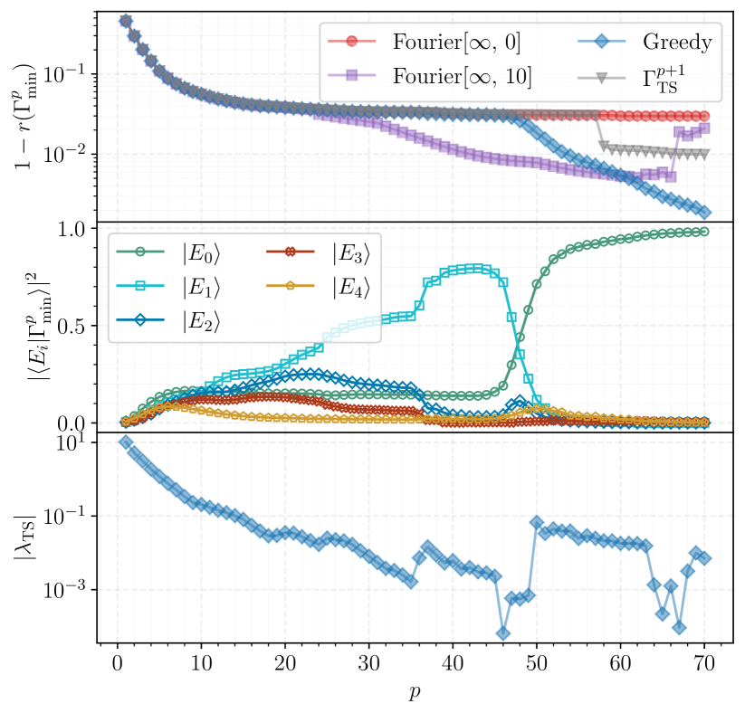
Figure 9: (Top) Behavior of the approximation ratio as a function of the circuit depth, for different optimization strategies. (Middle) Probability of measuring the fifth lowest energy eigenstates as a function of the circuit depth for the Greedy strategy. The ground state population remains unchanged for a wide range of circuit depths, followed by a sudden increase which correlates with the QAOA overcoming local minima. (Bottom) Circuit depth dependence of the landscape curvature at the transition state defined in Eq. (6) following the Greedy strategy. The curvature displays a gradual decrease, followed by a significant increase when the QAOA overcomes local minima.

In Fig. 9 we compare the performance of the QAOA under the Fourier$[\infty,0]$, Fourier$[\infty,10]$, Greedy, and $\Gamma^{p+1}_{\mathrm{TS}}$ strategies. From the approximation ratio, we note that all strategies yield the same performance for circuit depths $p\in[1,24]$, yet the improvement of the approximation ratio is stalled for $p\geq 10$. We attribute this behavior to the fact that QAOA prepares an excited state of the system with progressively increased fidelity, see the middle panel of Fig. 9. Eventually, however, the QAOA is able to escape the local minimum that prepares an excited state and starts converging to the ground state.

When the QAOA escapes the local minimum that prepares an excited state of the classical Hamiltonian depends on the initialization scheme. The initialization Fourier$[\infty,10]$ is the first to escape local optima at $p\sim 24$. Greedy follows next and only manages to escape around $p\sim 46$. Despite this, we observe that the final approximation is consistently better in Greedy than in all other strategies. Interestingly, we see that using only the first transition state as an initialization yields worse performance than Greedy and does escape the local minima that prepares the excited state but at circuit depths $p\sim 58$. Moreover, the initial variant of the Fourier strategy fails to escape from local optima and gets stalled for all circuit depths explored.

Following our comparative analysis, we articulate two critical observations. First, we conclude that QAOA is capable of preparing low-lying excited states of the classical Hamiltonian. How soon QAOA escapes from such a trap depends on the initialization scheme used, but this phenomenon is present for all initialization routines considered here. Second, we conclude that the landscape curvature at the initial transition state $\Gamma^{p+1}_{\mathrm{TS}}$, quantified in Eq. (10), is a good indicator of such QAOA behavior. Indeed, the bottom panel in Fig. 9 demonstrates that although the approximation ratio is stalling, the curvature keeps decreasing when QAOA prepares the excited state with progressively higher fidelity. As soon as QAOA starts converging to the true ground state, the curvature shows an increase and then continues to reduce.

All in all, our results suggest that there may be scenarios, particularly at large system sizes $N$, where the QAOA experiences stagnation, with negligible performance gains across a wide range of circuit depths $p$. This stagnation primarily arises because the QAOA effectively converges to a low-energy manifold of $H_{C}$, characterized by a small landscape curvature. In the context evaluated in this study Fig. 8, this manifold principally consists of the ground state and the first excited state Fig. 9. Our results suggest that the curvature provides useful insights into the QAOA behavior, complementary to the behavior of the approximation ratio.

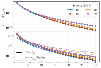
Figure 10: (Top) Circuit depth dependence of the approximation ratio $r(\Gamma^{p}_{\min})$. The scaling of the approximation ratio with the circuit depth $p$ matches the numerical results from [23]. (Bottom) Relationship between the magnitude of the negative curvature around the transition state $\Gamma^{p+1}{\mathrm{TS}}$ and the energy variance $\mathrm{var}_{\Gamma^{p}_{\min}}[H_{C}]$ as functions of circuit depth $p$. Although there appears to be qualitative agreement between the curvature and the energy variance across varying system sizes $N$, it is not as close as for the unweighted instances.

A.4 Numerical results for weighted 3-regular graphs

In this section we present numerical results analogous to those shown in the main text, but for weighted instances of MaxCut on 3-regular graphs.

We start by examining the curvature of the QAOA energy landscape at the transition state from Eq.(6), alongside the variance of the cost Hamiltonian in the QAOA state. In Fig. 10 we notice behavior similar to that for unweighted instances described in the main text, albeit with notable differences. First, the approximation ratio decays slower with the system size, aligning with findings from previous studies on similar MaxCut instances [23]. Second, while there is a close qualitative relationship between the energy variance of the QAOA state and the landscape curvature at the transition state in Eq. (6), this relationship is not as accurate as for unweighted instances, and energy variance decays slower compared to the curvature with QAOA depth $p$.

Finally, we check the accuracy of the lower bound on energy improvement from Eq. (16). Similar to observations with unweighted MaxCut instances, the lower bound significantly underestimates the energy improvement achieved by QAOA between consecutive circuit depths. At the same time, the ratio between true energy improvement and our lower bound seems to be a universal function of $p$ across a broad range of system sizes considered here.

Appendix B Bounds on the Hessian eigenvalue and eigenvector.

In this Appendix, we first construct upper and lower bounds for the minimum Hessian eigenvalue at the TS. In the second part of the Appendix, we introduce an approximation for the eigenvector associated with the minimum Hessian eigenvalue and show that its expectation value provides a tighter upper bound for the minimum Hessian eigenvalue. For clarity, throughout this Appendix we focus on symmetric TS. That is, TS where the zero insertion is made at the same layer $l$ for $\beta$ and $\gamma$ components. We fully describe our construction for the case $l\in[2,p+1]$ and only provide the final expression for the remaining eigenvectors.

B.1 Bound on the minimum Hessian eigenvalue

Given $\Gamma_{\min}^{p}$, a local minima of QAOA_p, let $\Gamma_{\text{TS}}^{p+1}(l,l)$ be the TS constructed by padding the $l$-th layer of the QAOA_p circuit with zeros. For clarity, we will omit the layer index whenever possible.

The starting point is to apply a change of basis $P$ that takes the Hessian at $\Gamma_{\text{TS}}^{p+1}$ to the following generic form:

$$H(\Gamma_{\text{TS}}^{p+1})\mapsto H_{P}(\Gamma_{\text{TS}}^{p+1}) =P^{T}H(\Gamma_{\text{TS}}^{p+1})P$$ (20)

$$=\left(\begin{array}[]{cc}H(\Gamma_{\text{min}}^{p})&v(l,l)\\ v^{T}(l,l)&h(l,l)\end{array}\right).$$ (23)

Ref. [26] demonstrated that the $2p\times 2$ rectangular matrix $v(l,l)$ is constructed by taking the $l-1$-th and the $p+l$-th columns of $H(\Gamma_{\text{min}}^{p})$. Using this knowledge, we can apply a composition of two elementary transformations on the rows and columns of $H(\Gamma_{\text{min}}^{p})$. More specifically, let us define the following $D\times D$ matrices:

1. $R_{i,j}^{D}(m)$ is the identity matrix that has an additional non-zero entry $m$ in the $(i,j)$ position. Note that when applied on the left to a matrix $A$, the resulting matrix will have $[A]_{i,x}\mapsto[A]_{i,x}+m[A]_{j,x}$. The inverse of this matrix is simply $(R_{i,j}^{D}(m))^{-1}=R_{i,j}^{D}(-m)$

2. $C_{i,j}^{D}(m)$ is the identity matrix with an additional non-zero entry $m$ in the $(j,i)$ position. Note that $C_{i,j}^{D}(m)$=$(R_{i,j}^{D}(m))^{T}$.

Using the above definitions, we bring the Hessian at point $\Gamma_{\text{TS}}^{p+1}$ to a block diagonal form:

$$H_{\text{block}} =\mathcal{R}H(\Gamma_{\text{TS}}^{p+1})\mathcal{R}^{T}=\left(\begin{array}[]{cc}H(\Gamma_{\text{min}}^{p})&0\\ 0&\bar{h}\end{array}\right),$$ (26)

$$\mathcal{R} =R_{2(p+1),p+l}^{2(p+1)}(-1)R_{2p+1,l-1}^{2(p+1)}(-1),$$ (27)

$$\bar{h} =\left(\begin{array}[]{cc}0&\bar{b}\\ \bar{b}&0\end{array}\right),$$ (30)

where

$$\bar{b} =\partial_{\beta_{l}}\partial_{\gamma_{l}}E(\Gamma^{p+1}_{l,l})-\partial_{\beta_{l-1}}\partial_{\gamma_{l}}E(\Gamma^{p}_{\min}),$$ (31)

$$=\langle+|U^{\dagger}[H_{C},U_{\geq l}[H_{C},H_{B}]U^{\dagger}_{\geq l}]U|+\rangle.$$ (32)

The transformation defined above subtracts rows $l-1$ and $p+l$ of $H(\Gamma_{\text{min}}^{p})$ to the first and second row of $v^{T}$ respectively. Then, we apply the same operation but on the columns. It is important to note that the eigenvalues of $H_{P}(\Gamma_{\text{TS}}^{p+1})$ do change under $\mathcal{R}$. This is because the transformation we applied is not a similarity transformation. To see this, note that by definition $\mathcal{R}^{T}\neq\mathcal{R}^{-1}$. However, we can use this block diagonal form to get some useful information on the minimum eigenvalue of $H_{P}(\Gamma_{\text{TS}}^{p+1})$. Recall the definition of the minimum eigenvalue of a squared matrix $M$ is

$$\lambda_{\text{min}}(M)=\text{inf}_{\|\psi\|=1}\langle\psi|M|\psi\rangle.$$

Using this definition on $\lambda_{\text{min}}(H_{\text{block}})$ we get

$$\lambda_{\text{min}}(H_{\text{block}}) =\inf_{\|\psi\|=1}\langle\psi|H_{\text{block}}|\psi\rangle,$$

$$=\inf_{\|\psi\|=1}\langle\psi|\mathcal{R}H_{P}(\Gamma_{\text{TS}}^{p+1})\mathcal{R}^{T}|\psi\rangle.$$

Multiplying by 1 in the form of $\|\mathcal{R}^{T}|\psi\rangle\|^{2}_{2}/\|\mathcal{R}^{T}|\psi\rangle\|^{2}_{2}$ and further using that

$$\|\mathcal{R}^{T}|\psi\rangle\|_{2}\leq\|\mathcal{R}^{T}\|_{2}\||\psi\rangle\|_{2}=\|\mathcal{R}^{T}\|_{2},$$

we obtain

$$\|\mathcal{R}^{T}\|_{2}^{-2}\lambda_{\text{min}}(H_{\text{block}})\geq\lambda_{\text{min}}(H_{P}(\Gamma_{\text{TS}}^{p+1})).$$ (33)

Doing the same on $\lambda_{\text{min}}(H_{P}(\Gamma_{\text{TS}}^{p+1}))$ we get

$$\lambda_{\text{min}}(H_{P}(\Gamma_{\text{TS}}^{p+1}))\geq\|(\mathcal{R}^{-1})^{T}\|_{2}^{2}\lambda_{\text{min}}(H_{\text{block}}).$$ (34)

In conclusion, by utilizing the fact that $H(\Gamma_{\text{TS}}^{p+1})$ and $H_{P}(\Gamma_{\text{TS}}^{p+1})$ possess identical spectra, we can establish the following bounds for the minimum eigenvalue of the Hessian at the TS

$$-\|(\mathcal{R}^{-1})^{T}\|_{2}^{2}|\bar{b}|\leq\lambda_{\text{min}}(H(\Gamma_{\text{TS}}^{p+1}))\leq-\|\mathcal{R}^{T}\|_{2}^{-2}|\bar{b}|,$$ (35)

where we used that $\lambda_{\text{min}}(H_{\text{block}})=-|\bar{b}|$. With the above inequalities, the bound on the minimum eigenvalue reduces to obtaining the operator norm of $\mathcal{R}$. This is, in general, a tough task but due to the simple form of the matrix $\mathcal{R}$ defined in Eq. (27) in this particular case, we can compute it. The operator norm is the maximum singular value of $\mathcal{R}$, which equivalently corresponds to the maximum eigenvalue of $\mathcal{R}\mathcal{R}^{T}$, which we can easily compute. In particular, we calculate the spectrum of the matrix $\mathcal{R}\mathcal{R}^{T}$ to consist of three different eigenvalues, $\sqrt{\frac{1}{2}(3+\sqrt{5})},\sqrt{\frac{1}{2}(3-\sqrt{5})}$ and $1$, with multiplicities $2,2$ and $2p-2$ respectively. Thus, we obtain that

$$|\mathcal{R}\|_{2}=\sqrt{\frac{1}{2}(3+\sqrt{5})}.$$ (36)

The same is true for the inverse of $\mathcal{R}$. With this, we arrive at the following bound

$$-\frac{3+\sqrt{5}}{2}|\bar{b}|\leq\lambda_{\text{min}}(H(\Gamma_{\text{TS}}^{p+1}))\leq-\frac{2}{3+\sqrt{5}}|\bar{b}|.$$ (37)

This provides upper and lower bounds on the magnitude of the minimum Hessian eigenvalue at the TS. Below, we introduce an approximation for the eigenvector associated with the minimum Hessian eigenvalue. Moreover, we show that the corresponding Rayleigh coefficient improves the upper bound provided in Eq. (37).

B.2 Eigenvector approximation

We define an analogous matrix to $\mathcal{R}$ in Eq. (27) that acts on columns:

$$\mathcal{C}=C_{2(p+1),p+l}^{2(p+1)}(-1/2)C_{2p+1,l-1}^{2(p+1)}(-1/2).$$ (38)

We now apply the transformation $\mathcal{R}^{-1}\mathcal{C}$ to $H_{P}(\Gamma_{\text{TS}}^{p+1})$, which gives the following expression:

$$\tilde{H}_{P}(\Gamma_{\text{TS}}^{p+1})=\mathcal{C}^{-1}\mathcal{R}H_{P}(\Gamma_{\text{TS}}^{p+1})\mathcal{R}^{-1}\mathcal{C}\\ =\left(\begin{array}[]{cc}H(\Gamma_{\text{min}}^{p})+M&0\\ 0&\bar{h}/2\end{array}\right)+\left(\begin{array}[]{cc}0&{u^{T}}/{4}\\ u&0\end{array}\right).$$ (39)

The matrix $M$ features two non-zero columns at indices $j=l-1$ and $j=p+l$, mirroring the structure of the Hessian matrix at the local minimum, $H(\Gamma_{\text{min}}^{p})$. It includes an additive correction of $\bar{b}/2$ at specific elements $M_{l-1,p+l}$ and $M_{p+l,l-1}$. More specifically,

$$M_{i,j}=H(\Gamma_{\text{min}}^{p})_{i,j}\Big{(}\delta_{j,l-1}\big{(}1+\frac{\bar{b}}{2}\delta_{i,p+l}\big{)}\\ +\delta_{j,p+l}\big{(}1+\frac{\bar{b}}{2}\delta_{i,l-1}\big{)}\Big{)}.$$ (40)

Finally, we have the $2\times 2p$ matrix $u$ with non zero entries equal to $\bar{b}$ at positions $\{1,p+l\}$ and $\{2,l-1\}$. It is important to note that the applied transformation here, in contrast to the one constructed in Eq. (27), is a similarity transformation. Thus, it preserves the spectrum of the Hessian while the eigenvectors are transformed as $v\mapsto\tilde{v}:=\mathcal{C}^{-1}\mathcal{R}v$.

We then define the approximate Hessian eigenstate to be

$$\tilde{v}_{\rm{bound}}=\left(\begin{array}[]{c}\bm{0}_{2p}\\ 1/\sqrt{2}\\ -\operatorname{sign}(\bar{b})/\sqrt{2}\end{array}\right).$$ (44)

Computing the expectation value of the Hessian on $\tilde{v}_{\rm{bound}}$ we get:

$$\lambda_{\mathrm{TS}}=-\absolutevalue{\bar{b}}/2,$$ (45)

which, taking into account that $\frac{1}{2}>\frac{2}{3+\sqrt{5}}$, improves the previously obtained upper bound on the minimum Hessian eigenvalue at the TS in Eq. (37)

$$-\frac{3+\sqrt{5}}{2}|\bar{b}|\leq\lambda_{\min}(H(\Gamma^{p+1}_{\rm{TS}}))\leq\lambda_{\mathrm{TS}}=-\frac{|\bar{b}|}{2}.$$ (46)

The last step is then to find the expression of $\tilde{v}_{\rm{bound}}$ in the original basis $\delta_{\rm{TS}}=P^{T}\mathcal{R}^{-1}\mathcal{C}\tilde{v}_{\rm{bound}}$, that results in the following form

$$[\delta_{\rm{TS}}]_{j}=\begin{cases}\frac{1}{2}&\text{if }j=l-1,l\\ -\frac{\operatorname{sign}(\bar{b})}{2}&\text{if }j=p+l+1,\\ \frac{\operatorname{sign}(\bar{b})}{2}&\text{if }j=p+l+2,\\ 0&\text{otherwise}.\end{cases}$$ (47)

Thus, we see that the approximate Hessian eigenvector has weights at layer $l$ as well as the two adjacent gates. The sparse structure of $\bm{\delta}_{\rm{TS}}$ comes from the fact that $\mathcal{R}^{-1}\mathcal{C}$ has only four non-zero offdiagonal matrix elements in positions $(2(p+1),p+l),(2p+1,l-1),(p+l,2(p+1))$, and $(l-1,2p+1)$. Thus, we see that when acting $\tilde{v}_{\rm{bound}}$, we will get a vector with also four non-zero elements. Since $\mathcal{R}^{-1}\mathcal{C}$ is not an orthogonal matrix, then it is needed to normalize the resulting vector $\mathcal{R}^{-1}\mathcal{C}\tilde{v}_{\rm{bound}}$. Finally, the action of the permutation will just reorder the elements in the vector without changing its content.

Finally, we list without derivation eigenvector and eigenvalue approximations for the remaining TS:

1. For $l=1$ we have that:

   $$[\delta_{\rm{TS}}]_{j}=\begin{cases}-\frac{\operatorname{sign}(b)}{\sqrt{2}}&\text{if }j=l,\\ \frac{1}{2}&\text{if }j=p+1+l,\\ -\frac{1}{2}&\text{if }j=p+1+l+1,\\ 0&\text{otherwise}.\end{cases}$$ (48)

   with $b=\langle+|[H_{C},[H_{B},U(\Gamma^{p}_{\min})^{\dagger}H_{C}U(\Gamma^{p}_{\min})]]|+\rangle$. The approximate eigenvalue in this case equals $-\absolutevalue{b}/\sqrt{2}$.

2. For $l=p+1$ we have that:

   $$[\delta_{\rm{TS}}]_{j}=\begin{cases}\frac{\operatorname{sign}(b)}{2}&\text{if }j=l-1,\\ -\frac{\operatorname{sign}(b)}{2}&\text{if }j=l,\\ \frac{1}{\sqrt{2}}&\text{if }j=p+1+l,\\ 0&\text{otherwise}.\end{cases}$$ (49)

   with $b=\langle+|U(\Gamma^{p}_{\min})^{\dagger}|[H_{C},[H_{B},H_{C}]]U(\Gamma^{p}_{\min})|+\rangle$. The approximate eigenvalue in this case equals $-\absolutevalue{b}/\sqrt{2}$.

We emphasize that the TS with $l=1$ and $l=p+1$ where the identity gates are inserted at the edges of the optimized QAOA circuit are special since the bound has prefactor $1/\sqrt{2}$ in contrast to the remaining TS where the bound features a prefactor $1/2$. We also emphasize this by using a constant $b$ rather than $\bar{b}$ used for the “bulk” transition states.

In the next section, we will use the eigenvector approximation Eq. (48) to derive a lower bound on the energy gain after each iteration of the QAOA algorithm. However, it is essential that before we obtain a simplified expression for $b=\langle+|[H_{C},[H_{B},U(\Gamma^{p}_{\min})^{\dagger}H_{C}U(\Gamma^{p}_{\min})]]|+\rangle$. This simplification leverages the specific forms of the mixing Hamiltonian $H_{B}$ and the cost Hamiltonian $H_{C}$. We use the fact that both states $|+\rangle$ and $H_{C}|+\rangle$ are eigenvectors of the mixing Hamiltonian $H_{B}$ with eigenvalues $-N$ and $-N+4$ respectively. This allows us to simplify the expression for $\bar{b}$ and arrive at the equation:

$$b=8\langle+|\tilde{H}_{C}H_{C}|+\rangle,$$ (50)

where $\tilde{H}_{C}=U(\Gamma^{p}_{\min})^{\dagger}H_{C}U(\Gamma^{p}_{\min})$ can be thought as the cost Hamiltonian in the Heisenberg picture. Furthermore, the condition $\partial_{\gamma_{1}}E(\Gamma^{p+1}_{\mathrm{TS}})=2\Im{\langle+|\tilde{H}_{C}H_{C}|+\rangle}=0$, which arises from the transition state being at a stationary point, is applied. It is important to note that the curvature in this scenario is described by $\lambda_{\mathrm{TS}}=-|b|/\sqrt{2}$, equivalently expressed as:

$$\lambda_{\mathrm{TS}}=-\operatorname{sign}(b)b/\sqrt{2}=-4\sqrt{2}|\langle+|\tilde{H}_{C}H_{C}|+\rangle|.$$ (51)

Appendix C Expansion of energy alongside the index-1 direction

Given a local minimum of QAOA_p, the transition states construction introduced in [26] guarantees that the energy has to decrease alongside the index-1 direction. Thus, in this section, we will use the approximate Hessian eigenvector introduced in Eq. (48) to provide a lower bound on the energy decrease after optimization of QAOA_p+1. Out of all possible $2p+1$ transition states available for a given local minima, we focus on the transition state constructed by inserting the zeros in the first layer of the QAOA circuit.

C.1 Energy

We begin by simplifying the expression for the QAOA_p+1 wave function obtained once we deviate from the transition state along the descent direction:

$$|\Gamma^{p+1}_{\text{TS}}+\varepsilon\bm{\delta}_{\text{TS}}\rangle=U(\Gamma^{p+1}_{\text{TS}}+\varepsilon\bm{\delta}_{\text{TS}})|+\rangle\\ =\Big{(}\prod_{l=1}^{p+1}U_{B}(\beta_{l})U_{C}(\gamma_{l})\Big{)}|+\rangle=U(\Gamma^{p}_{\min})U_{\varepsilon}|+\rangle,$$ (52)

where

$$U_{\varepsilon}=e^{-i\varepsilon/2H_{C}}e^{is_{b}\sqrt{2}\varepsilon/2H_{B}}e^{i\varepsilon/2H_{C}},$$ (53)

and we introduce a short-hand notation:

$$s_{b}=\operatorname{sign}(b).$$ (54)

The next step is to Taylor expand Eq. (53) around $\varepsilon=0$. For this, we will make use of the following identity:

$$e^{A}Be^{-A} =B+[A,B]+\frac{1}{2}[A,[A,B]]+\cdots$$ (55)

$$+\frac{1}{n!}[A,[A,\cdots[A,B]\cdots]].$$ (56)

Truncating the above expansion up to the 2nd order, and setting $B=e^{is_{b}\varepsilon\sqrt{2}H_{B}/2}$ and $A=-i\varepsilon H_{C}/2$ leads to

$$U_{\varepsilon}|+\rangle =e^{-i\varepsilon\phi}|+\rangle-i\frac{\varepsilon}{2}[H_{C},e^{is_{b}\varepsilon\sqrt{2}H_{B}/2}]|+\rangle$$ (57)

$$-\frac{\varepsilon^{2}}{2^{3}}[H_{C},[H_{C},e^{is_{b}\varepsilon\sqrt{2}H_{B}/2}]]|+\rangle,$$ (58)

where $\phi=s_{b}\sqrt{2}N/2$ and we used that $H_{B}|+\rangle=-N|+\rangle$.

To simplify the above expression we need to understand the action of the operator $e^{i\varepsilon\operatorname{sign}(b)\sqrt{2}H_{B}/2}$ on $H_{C}$ and $H_{C}^{2}$ operators. For this, it is important to note that $H_{C}|+\rangle$ is an eigenvector of $H_{B}$ with eigenvalue $(-N+4)$. With this at hand, we obtain that:

$$e^{is_{b}\varepsilon\sqrt{2}H_{B}/2}H_{C}|+\rangle=e^{is_{b}\varepsilon(-N+4)\sqrt{2}/2}H_{C}|+\rangle\\ =e^{-i\varepsilon\phi}e^{i\varepsilon s_{b}2\sqrt{2}}H_{C}|+\rangle.$$ (59)

The procedure is slightly more involved in the case of $H_{C}^{2}$. This is because $H_{C}^{2}$ is a sum of $4$-local, $2$-local, and $0$-local (constant) Hamiltonian densities. More specifically, the squared cost function Hamiltonian is written as

$$H_{C}^{2}=n_{C}^{2}\mathbb{I}+T_{2}+T_{4},$$ (60)

where $T_{k}$ with $k=2,4$ is a sum involving $4n_{\mathcal{E}}(\mathcal{G})$ and $n_{\mathcal{E}}(\mathcal{G})(n_{\mathcal{E}}(\mathcal{G})-5)$ $k$-local terms respectively. This, together with the $n_{\mathcal{E}}(\mathcal{G})$ terms contributing to $n_{C}^{2}\mathbb{I}$ makes for a total of $n_{\mathcal{E}}(\mathcal{G})^{2}$ terms. Thus, we obtain

$$e^{is_{b}\varepsilon\sqrt{2}H_{B}/2}H_{C}^{2}|+\rangle\\ =e^{-i\varepsilon\phi}(T_{0}\mathbb{I}+e^{i\varepsilon s_{b}2\sqrt{2}}T_{2}+e^{i\varepsilon s_{b}4\sqrt{2}}T_{4})|+\rangle\\ =e^{-i\varepsilon\phi}(H_{C}^{2}+(e^{i\varepsilon s_{b}2\sqrt{2}}-1)T_{2}+(e^{i\varepsilon s_{b}4\sqrt{2}}-1)T_{4})|+\rangle\\ =e^{-i\varepsilon\phi}H_{C}^{2}|+\rangle+e^{-i\varepsilon\phi}O_{\varepsilon}|+\rangle,$$ (61)

where we defined

$$O_{\varepsilon}=(e^{i\varepsilon s_{b}2\sqrt{2}}-1)T_{2}+(e^{i\varepsilon s_{b}4\sqrt{2}}-1)T_{4}).$$

Analogously, we obtain:

$$[H_{C},[H_{C},e^{-i\varepsilon s_{b}\sqrt{2}H_{B}/2}]]|+\rangle\\ =2e^{-i\varepsilon\phi}(1-e^{i\varepsilon s_{b}2\sqrt{2}})H_{C}^{2}|+\rangle+e^{-i\varepsilon\phi}O_{\varepsilon}|+\rangle.$$ (62)

Putting together Eq. (59), Eq. (61), and Eq. (62) we have a final expression for $U_{\varepsilon}|+\rangle$ that (up to a global phase) reads

$$U_{\varepsilon}|+\rangle=|+\rangle-i\frac{\varepsilon}{2}(1-e^{i\varepsilon s_{b}2\sqrt{2}})H_{C}|+\rangle\\ -\frac{\varepsilon^{2}}{2^{2}}(1-e^{i\varepsilon s_{b}2\sqrt{2}})H_{C}^{2}|+\rangle-\frac{\varepsilon^{2}}{2^{3}}O_{\varepsilon}|+\rangle.$$ (63)

We can then use Eq. (63) to obtain the expression for the energy when moving along the index-1 direction as a function of $\varepsilon$:

$$E(\Gamma^{p+1}_{\mathrm{TS}}+\varepsilon\delta_{\mathrm{TS}})=\langle+|U_{\varepsilon}^{\dagger}U^{\dagger}(\Gamma^{p}_{\min})H_{C}U(\Gamma^{p}_{\min})U_{\varepsilon}|+\rangle\\ =E(\Gamma^{p}_{\min})-\varepsilon\sin(2\sqrt{2}s_{b}\varepsilon)\langle+|\tilde{H}_{C}H_{C}|+\rangle\\ +\frac{\varepsilon^{2}}{2}\sin(\varepsilon s_{b}\sqrt{2})^{2}\partial^{2}_{\gamma_{1}}E(\Gamma^{p+1}_{\rm{TS}})\\ -\frac{\varepsilon^{2}}{2}\sin(\varepsilon 2\sqrt{2}s_{b})\Im{\langle+|\tilde{H}_{C}H_{C}^{2}|+\rangle}\\ -\frac{\varepsilon^{2}}{4}\Re{\langle+|\tilde{H}_{C}O_{\varepsilon}|+\rangle},$$ (64)

where for ease of notation we introduced $\tilde{O}=U^{\dagger}(\Gamma)OU(\Gamma)$ for a generic Hermitian operator $O$. The next step in the calculation is to isolate terms depending on the magnitude of their contribution with circuit depth $p$ (independently of the value of $\varepsilon$). For this, we need to further simplify the expectation value $\langle+|\tilde{H}_{C}O_{\varepsilon}|+\rangle$. After performing careful algebraic manipulations, we obtain a convoluted expression for the energy along the index-1 direction, represented as the fourth-order polynomial in the parameter $\varepsilon$. For enhanced readability, we present the terms of the expansion of $\Delta E(\varepsilon)=E(\Gamma^{p+1}_{\mathrm{TS}}+\varepsilon\delta_{\mathrm{TS}})-E(\Gamma^{p}_{\min})$ separately, organized according to the power of $\varepsilon$ with which they are associated:

$$\varepsilon^{2}\to -\varepsilon\sin(2\sqrt{2}s_{b}\varepsilon)\langle+|\tilde{H}_{C}H_{C}|+\rangle$$ (65)

$$\varepsilon^{3}\to -\frac{\varepsilon^{2}}{4}\sin(2\sqrt{2}s_{b}\varepsilon)\Im{\langle+|\tilde{H}_{C}T_{2}|+\rangle}-\frac{\varepsilon^{2}}{2}\sin(2\sqrt{2}s_{b}\varepsilon)\Big{(}1-\frac{\sin(4\sqrt{2}s_{b}\varepsilon)}{2\sin(2\sqrt{2}s_{b}\varepsilon)}\Big{)}\Im{\langle+|\tilde{H}_{C}T_{4}|+\rangle}.$$ (66)

$$\varepsilon^{4}\to \frac{\varepsilon^{2}}{2}\sin^{2}(\varepsilon s_{b}\sqrt{2})\partial^{2}_{\gamma_{1}}E(\Gamma^{p+1}_{\rm{TS}})+\frac{\varepsilon^{2}}{4}2\sin^{2}(\varepsilon s_{b}\sqrt{2})\Re{\langle+|\tilde{H}_{C}T_{2}|+\rangle}+\frac{\varepsilon^{2}}{2}\sin^{2}(2\varepsilon s_{b}\sqrt{2})\Re{\langle+|\tilde{H}_{C}T_{4}|+\rangle}.$$ (67)

From the above equations, we see that at the first non-trivial order in $\varepsilon$ the only cubical $\sim\varepsilon^{3}$ contribution that remains is $\Im{\langle+|\tilde{H}_{C}T_{2}|+\rangle}$. The quartic $\sim\varepsilon^{4}$ term is however more involved, and we resort instead to numerically verifying the order of magnitude of each term involved as a function of circuit depth $p$.

In Figure 12 we show the circuit depth dependence of three different terms, (1) $\partial^{2}_{\gamma_{1}}E(\Gamma^{p+1}_{\rm{TS}})$, (2) $\Re{\langle+|\tilde{H}_{C}T_{2}|+\rangle}$ and (3) $\Re{\langle+|\tilde{H}_{C}T_{4}|+\rangle}$ for a single MaxCut instance of a 3-regular weighted graph with $N=14$ vertices (see Fig. 8 for the details of the instance). The numerical data reveals that the term (1) $\partial^{2}_{\gamma_{1}}E(\Gamma^{p+1}_{\rm{TS}})$ dominates over terms (2)-(3) at all circuit depths.

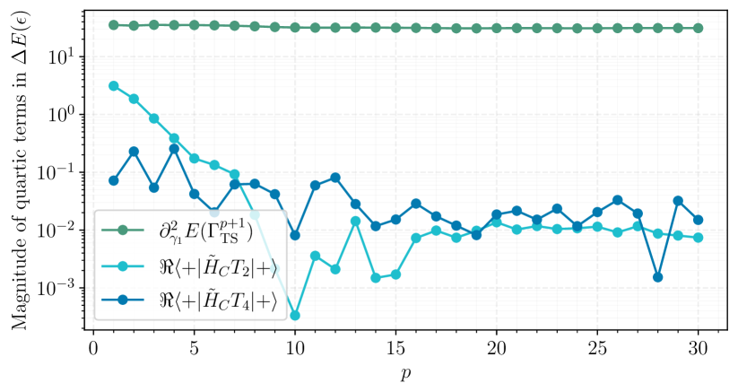
Figure 12: Magnitude of the prefactors of three different quartic terms $\sim\varepsilon^{4}$ in the energy expansion along the index-1 direction as a function of the circuit depth $p$. The first term in the expansion is dominant.

Finally, we obtain a close and concise expression for the energy change along the index-1 direction:

$$\Delta E(\varepsilon) \approx-\varepsilon\sin(2\sqrt{2}s_{b}\varepsilon)\langle+|\tilde{H}_{C}H_{C}|+\rangle$$

$$-\frac{\varepsilon^{2}}{4}\sin(2\sqrt{2}s_{b}\varepsilon)\Im{\langle+|\tilde{H}_{C}T_{2}|+\rangle}$$

$$+\frac{\varepsilon^{2}}{2}\sin^{2}(\varepsilon s_{b}\sqrt{2})\partial^{2}_{\gamma_{1}}E(\Gamma^{p+1}_{\rm{TS}}).$$ (68)

It is worth noting that in the above equation, Eq. (C.1) the quadratic term at small $\varepsilon$ is negative and proportional to the (approximate) minimum curvature, i.e,

$$\varepsilon^{2}\to-\varepsilon^{2}2\sqrt{2}\operatorname{sign}(b)b=\varepsilon^{2}\frac{\lambda_{\mathrm{TS}}}{2}.$$ (69)

The negative value of the second order term provided that the fourth order term is positive (see discussion in Sec. IV.2 after Eq. (IV.2)), leads to an existence of non-trivial minimum in the expansion of the energy along the index-1 direction. Our argument as to why $\partial^{2}_{\gamma_{1}}E(\Gamma^{p+1}_{\rm{TS}})>0$ lies on the observation that it can be approximated as the positive energy difference (see Eq. (IV.2)) of the states $\frac{1}{n_{C}}UH_{C}|+\rangle$ and $U|+\rangle$.

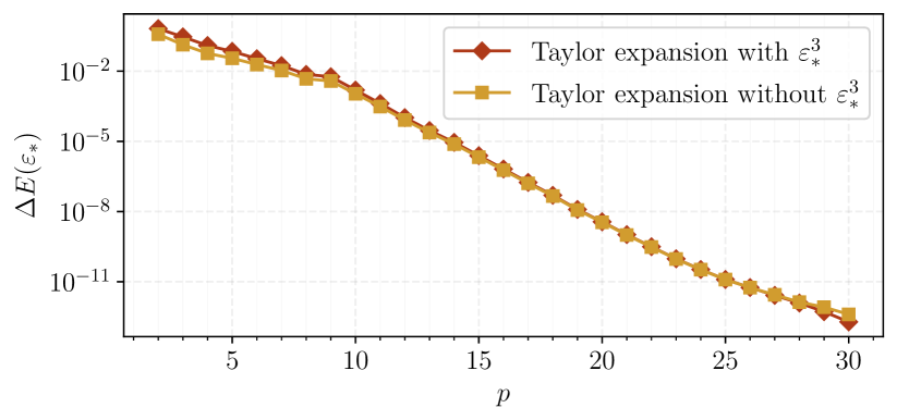
Figure 13: The energy difference between the transition state and the local minima obtained along the descent direction shows little sensitivity to the presence of the cubic term in the expansion.

As discussed in the main text, we discard the cubic $\sim\varepsilon^{3}$ term for simplicity. This approximation is justified by the negligible effect of the cubic term in the minima of the energy along the index-1 direction, as shown in Fig. 13. We are then left with an expression for the energy $\Delta E(\varepsilon)_{\rm{sym}}$ which has two degenerate global minima

$$\Delta E(\varepsilon^{*})_{\rm{sym}} =-\frac{\lambda_{\mathrm{TS}}^{2}}{16\partial^{2}_{\gamma_{1}}E(\Gamma^{p+1}_{\mathrm{TS}})},$$ (70)

where $(\varepsilon^{*})^{2}=-\lambda_{\mathrm{TS}}/4\partial^{2}_{\gamma_{1}}(\Gamma^{p+1}_{\mathrm{TS}})$.

References

- Cerezo et al. [2021] M. Cerezo, A. Arrasmith, R. Babbush, S. C. Benjamin, S. Endo, K. Fujii, J. R. McClean, K. Mitarai, X. Yuan, L. Cincio, and P. J. Coles, Variational quantum algorithms, Nature Reviews Physics 3, 625–644 (2021).
- Bharti et al. [2022] K. Bharti, A. Cervera-Lierta, T. H. Kyaw, T. Haug, S. Alperin-Lea, A. Anand, M. Degroote, H. Heimonen, J. S. Kottmann, T. Menke, W.-K. Mok, S. Sim, L.-C. Kwek, and A. Aspuru-Guzik, Noisy intermediate-scale quantum algorithms, Rev. Mod. Phys. 94, 015004 (2022).
- Preskill [2018] J. Preskill, Quantum Computing in the NISQ era and beyond, arXiv e-prints , arXiv:1801.00862 (2018), arXiv:1801.00862 [quant-ph] .
- Farhi et al. [2014] E. Farhi, J. Goldstone, and S. Gutmann, A Quantum Approximate Optimization Algorithm, arXiv e-prints , arXiv:1411.4028 (2014), arXiv:1411.4028 [quant-ph] .
- Peruzzo et al. [2014] A. Peruzzo, J. McClean, P. Shadbolt, M.-H. Yung, X.-Q. Zhou, P. J. Love, A. Aspuru-Guzik, and J. L. O’Brien, A variational eigenvalue solver on a photonic quantum processor, Nature Communications 5, 4213 (2014), arXiv:1304.3061 [quant-ph] .
- Farhi et al. [2015] E. Farhi, J. Goldstone, and S. Gutmann, A quantum approximate optimization algorithm applied to a bounded occurrence constraint problem (2015), arXiv:1412.6062 [quant-ph] .
- Farhi et al. [2020] E. Farhi, D. Gamarnik, and S. Gutmann, The Quantum Approximate Optimization Algorithm Needs to See the Whole Graph: A Typical Case, arXiv e-prints , arXiv:2004.09002 (2020), arXiv:2004.09002 [quant-ph] .
- Boulebnane and Montanaro [2021] S. Boulebnane and A. Montanaro, Predicting parameters for the quantum approximate optimization algorithm for max-cut from the infinite-size limit (2021), arXiv:2110.10685 [quant-ph] .
- Boulebnane and Montanaro [2022] S. Boulebnane and A. Montanaro, Solving boolean satisfiability problems with the quantum approximate optimization algorithm (2022), arXiv:2208.06909 [quant-ph] .
- Brandão et al. [2018] F. G. S. L. Brandão, M. Broughton, E. Farhi, S. Gutmann, and H. Neven, For Fixed Control Parameters the Quantum Approximate Optimization Algorithm’s Objective Function Value Concentrates for Typical Instances, arXiv e-prints , arXiv:1812.04170 (2018), arXiv:1812.04170 [quant-ph] .
- Wurtz and Love [2021] J. Wurtz and P. Love, MaxCut quantum approximate optimization algorithm performance guarantees for , Phys. Rev. A 103, 042612 (2021), arXiv:2010.11209 [quant-ph] .
- Zhou et al. [2024] L. Zhou, J. Basso, and S. Mei, Statistical estimation in the spiked tensor model via the quantum approximate optimization algorithm (2024), arXiv:2402.19456 [quant-ph] .
- Basso et al. [2022a] J. Basso, D. Gamarnik, S. Mei, and L. Zhou, Performance and limitations of the qaoa at constant levels on large sparse hypergraphs and spin glass models, in 2022 IEEE 63rd Annual Symposium on Foundations of Computer Science (FOCS) (2022) pp. 335–343.
- Basso et al. [2022b] J. Basso, E. Farhi, K. Marwaha, B. Villalonga, and L. Zhou, The quantum approximate optimization algorithm at high depth for maxcut on large-girth regular graphs and the sherrington-kirkpatrick model (Schloss Dagstuhl – Leibniz-Zentrum für Informatik, 2022).
- Sureshbabu et al. [2024] S. H. Sureshbabu, D. Herman, R. Shaydulin, J. Basso, S. Chakrabarti, Y. Sun, and M. Pistoia, Parameter Setting in Quantum Approximate Optimization of Weighted Problems, Quantum 8, 1231 (2024).
- Yao et al. [2020] J. Yao, M. Bukov, and L. Lin, Policy gradient based quantum approximate optimization algorithm (2020), arXiv:2002.01068 [quant-ph] .
- Zhu et al. [2022] L. Zhu, H. L. Tang, G. S. Barron, F. A. Calderon-Vargas, N. J. Mayhall, E. Barnes, and S. E. Economou, An adaptive quantum approximate optimization algorithm for solving combinatorial problems on a quantum computer (2022), arXiv:2005.10258 [quant-ph] .
- Harrigan et al. [2021] M. P. Harrigan et al., Quantum approximate optimization of non-planar graph problems on a planar superconducting processor, Nature Physics 17, 332–336 (2021).
- Weidenfeller et al. [2022] J. Weidenfeller, L. C. Valor, J. Gacon, C. Tornow, L. Bello, S. Woerner, and D. J. Egger, Scaling of the quantum approximate optimization algorithm on superconducting qubit based hardware, arXiv e-prints , arXiv:2202.03459 (2022), arXiv:2202.03459 [quant-ph] .
- Wurtz et al. [2024] J. Wurtz, S. Sack, and S.-T. Wang, Solving non-native combinatorial optimization problems using hybrid quantum-classical algorithms (2024), arXiv:2403.03153 [quant-ph] .
- Ebadi et al. [2022] S. Ebadi et al., Quantum Optimization of Maximum Independent Set using Rydberg Atom Arrays, Science 376, 1209 (2022), arXiv:2202.09372 [quant-ph] .
- Crooks [2018] G. E. Crooks, Performance of the Quantum Approximate Optimization Algorithm on the Maximum Cut Problem, arXiv e-prints , arXiv:1811.08419 (2018), arXiv:1811.08419 [quant-ph] .
- Zhou et al. [2020] L. Zhou, S.-T. Wang, S. Choi, H. Pichler, and M. D. Lukin, Quantum approximate optimization algorithm: Performance, mechanism, and implementation on near-term devices, Phys. Rev. X 10, 021067 (2020).
- Sack and Serbyn [2021] S. H. Sack and M. Serbyn, Quantum annealing initialization of the quantum approximate optimization algorithm, arXiv e-prints , arXiv:2101.05742 (2021), arXiv:2101.05742 [quant-ph] .
- Jain et al. [2021] N. Jain, B. Coyle, E. Kashefi, and N. Kumar, Graph neural network initialisation of quantum approximate optimisation, arXiv e-prints , arXiv:2111.03016 (2021), arXiv:2111.03016 [quant-ph] .
- Sack et al. [2023] S. H. Sack, R. A. Medina, R. Kueng, and M. Serbyn, Recursive greedy initialization of the quantum approximate optimization algorithm with guaranteed improvement, Phys. Rev. A 107, 062404 (2023).
- Day et al. [2019] A. G. R. Day, M. Bukov, P. Weinberg, P. Mehta, and D. Sels, Glassy phase of optimal quantum control, Phys. Rev. Lett. 122, 020601 (2019).
- Broyden [1970] C. G. Broyden, The Convergence of a Class of Double-rank Minimization Algorithms 1. General Considerations, IMA Journal of Applied Mathematics 6, 76 (1970).
- Fletcher [1970] R. Fletcher, A new approach to variable metric algorithms, The Computer Journal 13, 317 (1970).
- Goldfarb [1970] D. Goldfarb, A family of variable-metric methods derived by variational means, Mathematics of Computation 24, 23 (1970).
- Shanno [1970] D. F. Shanno, Conditioning of quasi-newton methods for function minimization, Mathematics of Computation 24, 647 (1970).
- Bezanson et al. [2017] J. Bezanson, A. Edelman, S. Karpinski, and V. B. Shah, Julia: A fresh approach to numerical computing, SIAM Review 59, 65 (2017), https://doi.org/10.1137/141000671 .
- Medina [2024] R. A. Medina, QAOALandscapes.jl, https://github.com/RaimelMedina/QAOALandscapes/tree/main (2024).
- Besard et al. [2018] T. Besard, C. Foket, and B. De Sutter, Effective extensible programming: Unleashing Julia on GPUs, IEEE Transactions on Parallel and Distributed Systems 10.1109/TPDS.2018.2872064 (2018), arXiv:1712.03112 [cs.PL] .
- Besard et al. [2019] T. Besard, V. Churavy, A. Edelman, and B. De Sutter, Rapid software prototyping for heterogeneous and distributed platforms, Advances in Engineering Software 132, 29 (2019).
- [36] T. Besard and M. Hawkins, Metal.jl, available online at https://github.com/JuliaGPU/Metal.jl.
- Mogensen and Riseth [2018] P. K. Mogensen and A. N. Riseth, Optim: A mathematical optimization package for julia, Journal of Open Source Software 3, 615 (2018).
- Mogensen et al. [2024] P. K. Mogensen, J. M. White, A. N. Riseth, T. Holy, M. Lubin, C. Stocker, A. Noack, A. Levitt, C. Ortner, B. Legat, B. Johnson, C. Rackauckas, Y. Yu, K. Carlsson, D. Lin, A. Strouwen, J. Grawitter, T. Arakaki, B. Pasquier, T. R. Covert, R. Rock, M. Creel, cossio, J. Regier, B. Kuhn, A. Stukalov, A. Williams, and K. Sato, Julianlsolvers/optim.jl: v1.9.3+doc1 (2024).
- Luo et al. [2020] X.-Z. Luo, J.-G. Liu, P. Zhang, and L. Wang, Yao.jl: Extensible, efficient framework for quantum algorithm design, Quantum 4, 341 (2020).
- Jones and Gacon [2020] T. Jones and J. Gacon, Efficient calculation of gradients in classical simulations of variational quantum algorithms (2020), arXiv:2009.02823 [quant-ph] .