Source identification using different moment hierarchies

Abstract

This work considers the localization of a bioluminescent source in a tissue-mimicking phantom. To model the light propagation in the resulting inverse problem the radiative transfer equation is approximated by using hierarchical simplified moment approximations. The inverse problem is then solved by using a consensus-based optimization algorithm.

1 Introduction

Bioluminescence imaging (BLI) is a widely used method for tracking cells, either to monitor tumor or pathogen growth and for assessing gene expression with reporter genes [27]. Usually, image acquisition is fast and has low background noise due to its high specificity. However, to find the source of light, 3D tomographic reconstruction models need to be applied, which require coupling with anatomical and optical information as well as numerical simulation to compute the diffuse light propagation from the source of light to the camera.
The radiative transfer equation (RTE) [6] is a well-known model for the propagation of light in heterogeneous media, and, optical tomography problems have been considered using the RTE e.g. in the mathematical community [2]. Its numerical approximation usually follows a semi-discretization applied in the angular direction with two major approaches: discrete ordinate methods and moment methods. Discrete ordinate methods apply quadrature formulas on the sphere [6, 17] and those methods are closely related to Galerkin methods [31, 18]. Iterative solvers are used to solve the resulting set of algebraic equations [1]. On the other hand, moment methods are typically based on truncated spherical harmonic expansions using variational discretization strategies [24, 8] or, for the time-dependent RTE, finite difference methods [30].
In applications, a diffusive approximation of the RTE is often employed if the scattering is dominant. So far, only this approach has been considered for finding the light source in BLI, see e.g. [13, 7, 16, 14, 19]. To the best of the authors’ knowledge, higher-order moment methods have not yet been applied. However, moment hierarchies have been effectively used in other inverse problems related to RTE, such as in radiotherapy treatment [10, 15]. This study suggests discretized moment hierarchies to localize a BLI light source.

2 Mathematical modeling

2.1 Radiative transfer equation

Light propagation in heterogeneous media is described by RTE with an (unknown) isotropic source term $q(x)$, i.e., the light source.

$$\Omega\nabla_{x}\psi(x,\Omega)+\Sigma_{t}(x)\psi(x,\Omega)= \int_{S^{2}}s(x,\Omega\cdot\Omega^{\prime})\psi(x,\Omega^{\prime})d\Omega^{\prime} +q(x)$$ (1)

The angular flux $\psi\in\mathbb{R}$ describes the (light) particle density at space coordinate $x\in\mathcal{P}\subset\mathbb{R}^{3},$ $\mathcal{P}$ being a convex phantom, and traveling in direction $\Omega\in S^{2}$, where $S^{2}$ is the unit sphere in 3D. The particles undergo scattering and absorption in the heterogenous medium. The parameters are defined as follows: $\Sigma_{t}:=\Sigma_{s}+\Sigma_{a}$ is the total cross section with the absorption cross section $\Sigma_{a}$ and scattering cross section $\Sigma_{s}$. The values are defined below and depend on the phantom used. The scattering kernel $s$ is normalized and for an isotropic scattering given by $s(x,\nu)=\frac{1}{4\pi}\Sigma_{s}(x)$. The scattering and absorption parameters are given by

$$\Sigma_{a}(x)=\mu_{a}(\lambda)\chi_{\mathcal{P}}(x)\quad\text{and}\quad\Sigma_{s}(x)=\mu_{s}^{\prime}(\lambda)\chi_{\mathcal{P}}(x),$$

where $\lambda$ is the wavelength, the scattering and absorption parameters depend on the material of the phantom, and $\chi_{\mathcal{P}}(x)$ is the characteristic function. Boundary conditions for $\psi$ are given by vacuum boundary conditions due to the setup described below, i.e., $\psi(x,\Omega)=0$ for $(x,\Omega)\in\partial\mathcal{P}\times S^{2}$ and $n(x)\cdot\Omega<0$, where $n$ is the normal vector.

2.2 Inverse problem

Our goal is to identify a bioluminescent light source $q$ in a phantom, given reference measurements (data) $U_{ref}(\lambda)$ at the boundary of the probe $\partial\mathcal{P}.$ In particular, we will use bioluminescence images which are available for a selected number of wavelengths $\lambda$. The source is modeled by a quadrilateral $\mathcal{Q}$ – a not self-intersecting four-sided polygon at a depth of $X_{0}$. The latter can be described by its eight corners $X_{i},i=2,\dots,9.$ The intensity of the source $X_{1}=\max_{x}q(x)$ is unknown, too:

$$\mathcal{X}= \{X\in\mathbb{R}^{9}|X_{1}>0,\text{ the points }(X_{2i},X_{2i+1}),\ i=1,\dots,4\text{ define a quadrilateral }\mathcal{Q}\subset\mathcal{P}\}.$$

The depth coordinate $X_{0}$ will be identified using the absorption rates below. For $X\in\mathcal{X}$ the source $q(x)$ is then given by

$$q_{X}(x)=X_{1}\cdot\chi_{\mathcal{Q}}(x).$$

The scalar flux is given by $\psi_{0}(\cdot)=\int_{S^{2}}\psi(\cdot,\Omega^{\prime})d\Omega^{\prime}$ denoted in the following by $\psi_{0}(\cdot,\lambda,X)$.
For each fixed $\lambda,$ the inverse problem is given by

$$\min_{X\in\mathcal{X},X_{0}}f(X):=\|U_{ref}(\lambda)-\psi_{0}(\cdot,\lambda,X)\|_{L^{2}(\partial\mathcal{P})}$$ (2)

subject to (1)

The previous formulation holds for $x\in\mathbb{R}^{3}$ and data $U_{ref}$ available at the surface of the probe, see e.g. [13, 7, 16, 14, 19] for diffusive approximations to solve the previous problem.
Our approach comprises the following steps: We reduce the problem and assume that $\Sigma_{a}$ and $\Sigma_{s}$ do not depend on the depth $X_{0}$ of the probe. Then, the RTE is solved for $\psi=\psi(x,\Omega)$ for $x\in\mathbb{R}^{2}$ reducing the computational overhead. The first step provides the position of the light source in a 2D cross section as solution to the following problem in two spatial dimensions:

$$\min_{X\in\mathcal{X}}f(X):=\|U_{ref}(\lambda)-\psi_{0}(\cdot,\lambda,X)\|_{L^{2}(\partial\mathcal{P})}$$ (3)

$$\text{ subject to \eqref{eq:RTE}}.$$

A hierarchy of simplified moment approximations is used to approximate the solutions to the RTE. In a second setup, the unknown depth is estimated, using the 1D formulation of the RTE (1) without scattering.

2.3 Hierarchical Simplified Moment Approximation

The RTE is posed in a 4D phase space (space $x$ and direction $\Omega$) rendering the simulation and subsequent optimization computationally expensive. Therefore, reduced models using a series expansion in the angular dependence with spherical harmonic functions are proposed [5, 30, 28]. The resulting spherical harmonic equations called $P_{N}$ equations, can be further simplified in the case of scattering media [11, 12, 25, 20]. We briefly describe the approach to derive the simplified $P_{N}$ ($SP_{N}$) equations, see also [15] for an extension towards inverse problems.
For simplicity, we follow the ad hoc approach considered in [11, 12] to derive a hierarchy of simplified models, see also [22, 30]. Starting from a 1D planar geometry the equations read

$$\alpha\partial_{y}\psi(y,\alpha,\beta)+\Sigma_{t}(y)\psi(y,\alpha,\beta)= \frac{\Sigma_{s}(x)}{4\pi}\int_{0}^{2\pi}\int_{-1}^{1}\psi(y,\alpha^{\prime},\beta^{\prime})d\alpha^{\prime}d\beta^{\prime}$$

$$+q(y).$$

By integrating with respect to $\alpha$ and $\beta$, multiplying by the Legendre polynomials $P_{n}(\alpha)$, and using their recursion relation, we can rewrite the equation in the following set of equations:

$$\partial_{y}\Big{(}\frac{n+1}{2n+1}\phi_{n+1}(y) +\frac{n}{2n+1}\phi_{n-1}(y)\Big{)}+\Sigma_{t}(y)=\delta_{n,0}(\Sigma_{s}(y)\phi_{0}(y)+4\pi q(y)),$$

where $\phi_{n}(y)=\int_{-1}^{1}P_{n}(\alpha^{\prime})\int_{0}^{2\pi}\psi(y,\alpha^{\prime},\beta^{\prime})d\beta^{\prime}d\alpha^{\prime}$. To simplify the equations, the set of equations is solved algebraically for every odd number of moments, and the solution is then inserted into the remaining ones. Finally, the 1D differential operator $\partial_{y}$ is formally replaced by the 2D operator $\nabla_{x}$. Exemplary, the 2D $SP_{1}$ equation is given by

$$-\frac{1}{3}\nabla_{x}\cdot\left(\frac{1}{\Sigma_{t}(x)}\nabla_{x}\phi_{0}(x)\right)+\Sigma_{a}(x)\phi_{0}(x)=4\pi q(x).$$

For our computational results we will consider $SP_{1}$ and $SP_{5}$ approximation. The scalar flux in (2) is the zeroth moment $\phi_{0}$ of each $SP_{N}$ approximation.
In step 1, we are interested in determining the location of the source in dimensions of the bioluminescent images. For step 2, we obtain an estimate of the depth. We will use a rather simple formula that provides satisfying results in our cases. We consider equation (1) only in the direction of the depth and neglect scattering, i.e. we set $\Omega=(0,0,1)^{T}$ and $\mu_{s}^{\prime}=0$. If we consider the parallel plane to the camera at the cylinder at $x_{3}=0$, then the unknown depth denoted by $X_{0}$ for each wavelength is given as

$$\psi(0)=e^{-\mu_{a}10^{3}X_{0}}\psi(X_{0})c.$$ (4)

Here, $10^{3}$ is due to converting the absorption rate to mm (from mm²), $\psi(0)$ is the maximum intensity value in $\mathcal{Q}$ of the reference data $U_{ref}(\lambda)$. The scaling parameter $c$ converts the unit of the reference data to the one of the emission intensity of the bioluminescent source $\psi(X_{0})$, which is obtained by an Infinite 200 Pro microplate reader. $\psi(0)$ can be obtained with the computed $\mathcal{Q}$ in step 1 for each wavelength and moment approximation. The scaling parameter $c$ (uniform over all examples) and $X_{0}$ (for each position and moment approximation) are unknown. We set the depth $X_{0}$ to be the same for all wavelengths. Hence, we solve a nonlinear curve-fitting problem in least-squares sense given by (4) and the data provided by the measurements and optimization results for different wavelengths and moment approximations.
The shape of the phantom in the transverse $x_{1}-x_{3}$ plane is a circle, see Figure 1(a). Hence, the calculated depth must be corrected by the distance between the boundary of the phantom and the parallel line to the camera at $0$, i.e. for $r_{\mathcal{P}}$ being the radius of the cylinder, $M^{x_{1}}_{\mathcal{P}}$ the midpoint of $\mathcal{P}$ in $x_{1}$ direction, we set

$$X_{0}\mapsto X_{0}+r_{\mathcal{P}}^{2}-\sqrt{r_{\mathcal{P}}^{2}-(\frac{1}{4}\sum_{i=1}^{4}X_{2i-1}-M^{x_{1}}_{\mathcal{P}})^{2}}.$$

3 Numerical results

3.1 Numerical approximation

The numerical solution to (1) is obtained using a staggered grid radiation moment approximation developed in [30] accessible at GitHub. The code uses pseudo-time stepping to solve the $SP_{N}$ approximation to the RTE (1). We provide zero initial data for the pseudo-time stepping algorithm and simulate until the $L^{2}$ norm of the (approximate) temporal derivative inside the phantom $\mathcal{P}$ is small, i.e. $\|\partial_{t}\phi_{0}\|_{L^{2}(\mathcal{P})}\leq\varepsilon.$ The method is second order in space (and pseudo-time) and we refer to [30] for additional implementational details. Vacuum boundary conditions are achieved by extending the computational domain such that no interaction with the boundaries occurs [30, Section 6.3].
To solve the inverse problem (3), we first discretize the differential equation and optimize the discrete formulation. The reference solutions are mapped onto the grid of the computational domain and the objective function is approximated by a midpoint quadrature leading to the discrete $\ell^{2}$ norm. To find the optimal value we use a consensus-based optimization (CBO) algorithm [23, 4, 3, 9]. This algorithm belongs to the class of stochastic particle optimization methods using $i=1,\dots,M$ particles $X^{i}\in\mathcal{X}.$ The system of particles evolves in pseudo-time $\tau$ following a stochastic differential equation, see e.g. [23]:

$$dX^{i}(\tau)=-\delta(X^{i}(\tau)-c_{f}^{\alpha}(X))d\tau+\sigma\text{diag}(X^{i}(\tau)-c_{f}^{\alpha}(X))dW^{i}(\tau).$$

In case particles leave the domain $\mathcal{X}$ we project them back by $X^{i}(t)=\text{argmin}\{\|X^{i}(t)-y\|,y\in\mathcal{X}\}$. The dynamics above are driven by two components: A drift part with strength $\delta\geq 0$ moves the particles towards the so-called consensus point $c_{f}^{\alpha}(X)$, which is given by

$$c_{f}^{\alpha}(X)=\frac{\sum_{i=1}^{M}X^{i}(t)\omega_{\alpha}^{f}(X^{i}(t))}{\sum_{i=1}^{M}\omega_{\alpha}^{f}(X^{i}(t))},\quad\omega_{\alpha}^{f}(x)=\exp(-\alpha f(x)),$$

and the anisotropic diffusion part allows for the exploration of the admissible domain $\mathcal{X}$ by using the Brownian motion $W^{i}$ and $\sigma\geq 0$. Under mild assumptions on $f(\cdot)$, it can be shown that $\frac{1}{M}\sum_{i=1}^{M}X_{i}(\tau)\to X^{*}$ for $\tau\to\infty$ converge towards the global minimizer of problem (3), see [9].

3.2 Experimental set-up

BLI is performed in a hybrid micro-CT optical imaging system (MILabs B.V., Houten, the Netherlands), by capturing the emitted light with a charge-coupled device (CCD) camera at 586 nm, 615 nm, 631 nm, and 661 nm with an acquisition time of approximately 2 minutes. After BLI, CT scans are performed in total body normal scan mode, tube voltage of 55 kV, tube current of 0.17 mA, an isotropic voxel size of 140 $\mu$m, and a scan time of 4 minutes. The reconstructed BLI data have an isotropic voxel size of 280 $\mu$m. The provided CT-aided BLI reconstruction (MILabs BLT Recon 1.0.2.3, developed by Gremse-IT GmbH, Aachen, Germany) takes into account structural information and wavelengths, is GPU-accelerated with a GeForce RTX 2080 Ti (NVIDIA, Santa Clara, CA), and takes approximately 4 minutes per scan.
The BLI phantom consists of $20\%$ gelatin (reinst, Silber, 140 Bloom, Carl Roth, Mannheim, Germany) with $5\%$ Lipovenoes MCT $20\%$ infusion solution (Fresenius Kabi, Bad Homburg, Germany) in water. It is cast into a 15 mL tube (Sarstedt Inc, Nümbrecht, Germany). After solidification, the length is adjusted to 3 cm, and a pipette tip containing 5 $\mu$L of the reactive solution of a red glow stick (Kontor3.11 GmbH, Chemnitz, Germany) is inserted into the phantom as described previously in [29]. The phantom is scanned in two positions, with a rotation of about 90° (see Figure 1(a) for the phantom in the holder). The emission intensity of the glow stick solution is measured at 586 nm, 615 nm, 631 nm, and 661 nm (bandwidth 20 nm) using an Infinite 200 Pro microplate reader (Tecan, Männedorf, Switzerland) to account for the relative brightness according to the wavelength. The values in arbitrary units are given by 183 (586 nm), 457 (615 nm), 421.5 (631 nm), and 382.5 (661 nm).
The absorption and scattering parameters are calculated based on formulas derived in [21]. The phantom is considered to consist of $5\%$ Lipovenoes MCT $20\%$ infusion solution (Fresenius Kabi, Bad Homburg, Germany) and $95\%$ water. As noted in [21], Lipovenoes MCT $20\%$ is low absorbing at visible wavelengths. For wavelengths larger than $500$ nm, the predominant absorber is water. The absorption of glycerin and egg lipid can be ignored due to the low concentration. The absorption of soybean oil has a low value for wavelength larger than $500$ nm, hence, it can be ignored, too. The absorption parameters for water can be found in [26]. The scattering parameters are approximated by [21, Eq. 10 and Table 4] for Lipovenoes $20\%$. The values are given in Table 1.

$\lambda$ (nm)	586	615	631	661
$\mu_{a}$ (cm-1)	1.1e-03	2.678e-03	2.916e-03	4.1e-03
$\mu_{s}^{\prime}$ (cm-1)	28.542	27.046	26.258	24.85

Table 1: Absorption and scattering parameters for different wavelengths

3.3 Results

To locate the sources in the two examples we choose a computational domain of size $5.5$ cm times $8$ cm. The boundary of the phantom $\partial\mathcal{P}$ is approximately a quadrilateral of size $1.5$ cm times $3$ cm placed in the middle of the computational domain. We use $n=350$ grid points in each direction. We consider $\varepsilon=$5e-03 as stopping criteria for the pseudo-time stepping algorithm. For the CBO algorithm we choose $\delta=1,\sigma=1$ and 500 particles. We stop the optimization after 100 iterations and use a pseudo-timestep of $0.1$ to solve the stochastic differential equation.

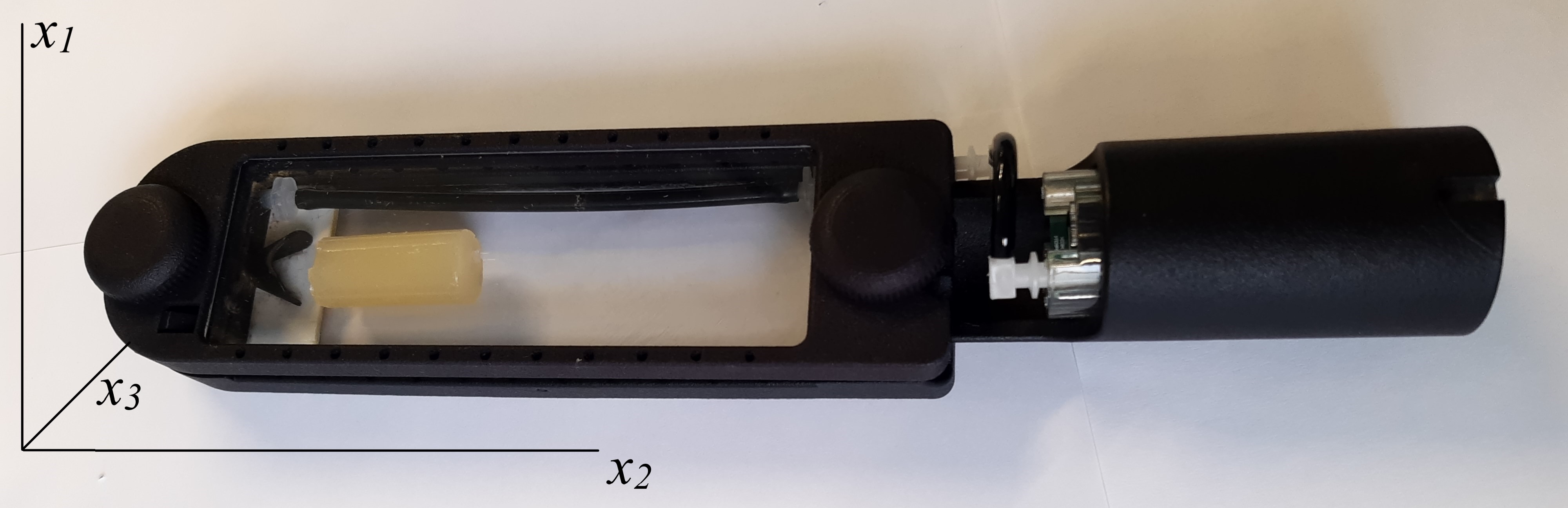
(a) Gelatin phantom in the optical imaging holder.

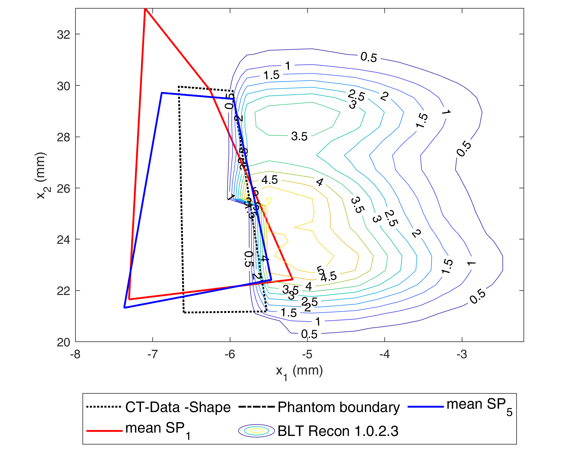
(b) Reconstructions for position 1

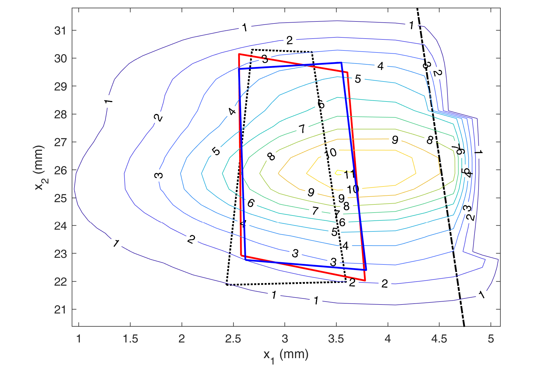
(c) Reconstructions for position 2

Figure 1: 1(a): Cylindrical gelatin phantom placed in an optical holder. 1(b) (Position 1) and 1(c) (Position 2): Comparison between the CT reconstruction (true shape) of the phantom in a black dotted line and reconstructions obtained through the proposed algorithm: The red solid line is the shape computed by the mean of each corner over all wavelengths for $SP_{1}$ and the blue solid line is the same for $SP_{5}$. The contour lines show the BLT 1.0.2.3 reconstruction. The black dash-dotted line (if visible) is the boundary of the phantom. The depth of each reconstruction is shown in Table 3.

Comparing the computed location of the sources obtained by $SP_{1}$ and $SP_{5}$, it can be noticed that particularly for the first data set (except for $\lambda=631$ nm) the approximation of the source is more accurate with $SP_{5}$. For this comparison, we compute the Euclidean distance of each corner with the CT data and compare the mean for each wavelength (Table 2). For the second data set the $SP_{1}$ approximation is already very close to the data such that $SP_{5}$ does not offer any real improvement for higher wavelengths.

$\lambda$ (nm)	Pos1 $SP_{1}$	Pos1 $SP_{5}$	Pos2 $SP_{1}$	Pos2 $SP_{5}$
586	1.9399	1.3602	1.0675	1.0173
615	4.6226	1.8674	0.84089	0.82037
631	1.2932	2.7726	0.43429	0.64835
661	2.028	1.394	0.42165	0.53004

Table 2: Mean deviation for different wavelengths in mm

By using (4) the obtained estimates for the depth can be found in Table 3. Although we use a rather simple formula it can be seen that we are close to the depth of the midpoint of the of the light source. In particular, we are closer than the source reconstruction using BLT 1.0.2.3 (with its brightest value as an estimate of the depth).

	$X_{0}$	BLT 1.0.2.3	CT-midpoint	CT-endpoints
Pos1: $SP_{1}$	0.8675	-0.48	0.72	$\pm 0.7$
Pos1: $SP_{5}$	0.5929	-0.48	0.72	$\pm 0.7$
Pos2: $SP_{1}$	3.8551	4.28	2.74	$\pm 0.5$
Pos2: $SP_{5}$	3.8530	4.28	2.74	$\pm 0.5$

Table 3: Different estimates for the depth in mm

Further, we compare our computed locations with the currently used BLT 1.0.2.3 reconstruction and the actual CT-determined positions (at the depths given by Table 3). Since we computed different approximations per wavelength for each moment methods, we compute the mean shape over all wavelengths. The results for the first position can be seen in Figure 1(b). The improvement by using higher moments can be seen immediately. Furthermore, the location is detected better than with BLT 1.0.2.3. The latter observation is also true for position two, see Figure 1(b): The location and shape are better approximated than with BLT 1.0.2.3. The improvements from $SP_{1}$ to $SP_{5}$ are less significant.

4 Discussion

The presented approach achieves a more accurate localization of the source by using higher order moments. Although we have only presented results in 2D, an extension to 3D is straightforward. It should be noted that the computational effort for the 3D localization of the source with $SP_{1}$ is the same as with the BLT 1.0.2.3 when the same optimization methods and discretization are used. For higher order moments the computational effort increases, since the system size of the reconstruction increases linearly as $(N+1)$. This displays the usual trade-off between accuracy and computational effort.
In contrast to the common applications of BLI, our approach is simplified to show the accuracy and possibilities of BLI reconstruction. In vivo, the heterogeneity of the sample would be higher in terms of the optical properties of tissues and by the potential for the light source to be located anywhere or at multiple points. The presented mathematical framework can be directly used to address these problems.
The proposed method can also be transferred to fluorescence tomography, but this requires extensions: These include reconstructing the light path from the excitation laser to the fluorescence source (including absorption and scattering), autofluorescence, and additional information on absorption and location obtained from laser excitation.
In summary, hierarchical calculations achieved more accurate localization, resulting in higher resolved images and ultimately better answers to research questions.

Funding

Deutsche Forschungsgemeinschaft (DFG, German Research Foundation): Project-IDs 403224013 (SFB 1382) and 525853336, 525842915, 526006304 (all SPP2410); European Union’s Horizon Europe research and innovation programme under the Marie Sklodowska-Curie Doctoral Network Datahyking: Grant No. 101072546

Disclosures

The authors declare no conflicts of interest.

Data Availability Statement

Data underlying the results presented in this paper are not publicly available at this time but may be obtained from the authors upon reasonable request.

References

- [1] Marvin L Adams and Edward W Larsen. Fast iterative methods for discrete-ordinates particle transport calculations. Progress in nuclear energy, 40(1):3–159, 2002.
- [2] Simon R Arridge and John C Schotland. Optical tomography: forward and inverse problems. Inverse problems, 25(12):123010, 2009.
- [3] Hyeong-Ohk Bae, Seung-Yeal Ha, Myeongju Kang, Hyuncheul Lim, Chanho Min, and Jane Yoo. A constrained consensus based optimization algorithm and its application to finance. Applied Mathematics and Computation, 416:126726, 2022.
- [4] Giacomo Borghi, Michael Herty, and Lorenzo Pareschi. Constrained consensus-based optimization. SIAM Journal on Optimization, 33(1):211–236, 2023.
- [5] Thomas A Brunner and James Paul Holloway. Two-dimensional time dependent riemann solvers for neutron transport. Journal of Computational Physics, 210(1):386–399, 2005.
- [6] Kenneth M Case, Paul F Zweifel, and GC Pomraning. Linear transport theory, 1968.
- [7] Abhijit J Chaudhari, Felix Darvas, James R Bading, Rex A Moats, Peter S Conti, Desmond J Smith, Simon R Cherry, and Richard M Leahy. Hyperspectral and multispectral bioluminescence optical tomography for small animal imaging. Physics in Medicine & Biology, 50(23):5421, 2005.
- [8] Herbert Egger and Matthias Schlottbom. A mixed variational framework for the radiative transfer equation. Mathematical Models and Methods in Applied Sciences, 22(03):1150014, 2012.
- [9] Massimo Fornasier, Timo Klock, and Konstantin Riedl. Convergence of anisotropic consensus-based optimization in mean-field law. In International Conference on the Applications of Evolutionary Computation, pages 738–754. Springer, 2022.
- [10] Martin Frank, Michael Herty, and Matthias Schäfer. Optimal treatment planning in radiotherapy based on boltzmann transport calculations. Mathematical Models and Methods in Applied Sciences, 18(04):573–592, 2008.
- [11] E M Gelbard. Applications of spherical harmonics method to reactor problems. Technical Report WAPD-BT-20, Bettis Atomic Power Laboratory, 1960.
- [12] E M Gelbard. Simplified spherical harmonics equations and their use in shielding problems. Technical Report WAPD-T-1182,, Bettis Atomic Power Laboratory, 1961.
- [13] Xuejun Gu, Qizhi Zhang, Lyndon Larcom, and Huabei Jiang. Three-dimensional bioluminescence tomography with model-based reconstruction. Optics express, 12(17):3996–4000, 2004.
- [14] Weimin Han and Ge Wang. Bioluminescence tomography: biomedical background, mathematical theory, and numerical approximation. Journal of computational mathematics, 26(3):324, 2008.
- [15] Michael Herty, Rene Pinnau, and Guido Thömmes. Asymptotic and discrete concepts for optimal control in radiative transfer. ZAMM Z. Angew. Math. Mech., 87(5):333–347, 2007.
- [16] Ming Jiang, Tie Zhou, Jiantao Cheng, Wenxiang Cong, and Ge Wang. Image reconstruction for bioluminescence tomography from partial measurement. Optics Express, 15(18):11095–11116, 2007.
- [17] Claes Johnson and Juhani Pitkäranta. Convergence of a fully discrete scheme for two-dimensional neutron transport. SIAM J. Numer. Anal., 20(5):951–966, 1983.
- [18] József Kópházi and Danny Lathouwers. A space–angle dgfem approach for the boltzmann radiation transport equation with local angular refinement. Journal of Computational Physics, 297:637–668, 2015.
- [19] Chaincy Kuo, Olivier Coquoz, Tamara L Troy, Heng Xu, and Brad W Rice. Three-dimensional reconstruction of in vivo bioluminescent sources based on multispectral imaging. J. Biomed. Opt., 12(2):024007–024007, 2007.
- [20] Edward W Larsen, Jim E Morel, and John M McGhee. Asymptotic derivation of the simplified p n equations. Proceedings of Joint International Conference on Mathematical Methods and Supercomputing in Nuclear Applications, 1993.
- [21] René Michels, Florian Foschum, and Alwin Kienle. Optical properties of fat emulsions. Optics express, 16(8):5907–5925, 2008.
- [22] Edgar Olbrant, Edward W Larsen, Martin Frank, and Benjamin Seibold. Asymptotic derivation and numerical investigation of time-dependent simplified pn equations. Journal of Computational Physics, 238:315–336, 2013.
- [23] René Pinnau, Claudia Totzeck, Oliver Tse, and Stephan Martin. A consensus-based model for global optimization and its mean-field limit. Mathematical Models and Methods in Applied Sciences, 27(01):183–204, 2017.
- [24] Juhani Pitkäranta. Approximate solution of the transport equation by methods of galerkin type. Journal of Mathematical Analysis and Applications, 60(1):186–210, 1977.
- [25] Gerald C Pomraning. Asymptotic and variational derivations of the simplified pn equations. Annals of nuclear energy, 20(9):623–637, 1993.
- [26] Robin M Pope and Edward S Fry. Absorption spectrum (380–700 nm) of pure water. ii. integrating cavity measurements. Applied optics, 36(33):8710–8723, 1997.
- [27] Ruxana T Sadikot and Timothy S Blackwell. Bioluminescence imaging. Proceedings of the American Thoracic Society, 2(6):537–540, 2005.
- [28] Matthias Schäfer, Martin Frank, and C. David Levermore. Diffusive corrections to approximations. Multiscale Model. Simul., 9(1):1–28, 2011.
- [29] Sarah Schraven, Ramona Brück, Stefanie Rosenhain, Teresa Lemainque, David Heines, Hormoz Noormohammadian, Oliver Pabst, Wiltrud Lederle, Felix Gremse, and Fabian Kiessling. Ct-and mri-aided fluorescence tomography reconstructions for biodistribution analysis. Investigative Radiology, 2023.
- [30] Benjamin Seibold and Martin Frank. Starmap—a second order staggered grid method for spherical harmonics moment equations of radiative transfer. ACM Transactions on Mathematical Software (TOMS), 41(1):1–28, 2014.
- [31] Todd A Wareing, John M McGhee, Jim E Morel, and Shawn D Pautz. Discontinuous finite element sn methods on three-dimensional unstructured grids. Nuclear science and engineering, 138(3):256–268, 2001.