Continuous Transfer Learning for UAV Communication-aware Trajectory Design

Abstract

Deep Reinforcement Learning (DRL) emerges as a prime solution for Unmanned Aerial Vehicle (UAV) trajectory planning, offering proficiency in navigating high-dimensional spaces, adaptability to dynamic environments, and making sequential decisions based on real-time feedback. Despite these advantages, the use of DRL for UAV trajectory planning requires significant retraining when the UAV is confronted with a new environment, resulting in wasted resources and time. Therefore, it is essential to develop techniques that can reduce the overhead of retraining DRL models, enabling them to adapt to constantly changing environments. This paper presents a novel method to reduce the need for extensive retraining using a double deep Q network (DDQN) model as a pre-trained base, which is subsequently adapted to different urban environments through Continuous Transfer Learning (CTL). Our method involves transferring the learned model weights and adapting the learning parameters, including the learning and exploration rates, to suit each new environment’s specific characteristics. The effectiveness of our approach is validated in three scenarios, each with different levels of similarity. CTL significantly improves learning speed and success rates compared to DDQN models initiated from scratch. For similar environments, Transfer Learning (TL) improved stability, accelerated convergence by 65%, and facilitated 35% faster adaptation in dissimilar settings.

I Introduction

UAVs are increasingly employed in a broad spectrum of applications, including surveillance, agriculture, disaster management, and communication infrastructure maintenance [1]. Efficient planning and optimization of UAV trajectories is critical, since the success of numerous UAV applications, such as real-time data transmission and remote sensing, heavily relies on a reliable trajectory. One of the key challenges in UAV trajectory is ensuring robust communication between UAVs and ground-based infrastructure, such as Base Stations. This challenge becomes even more pronounced in complex urban environments with obstacles and interference.

Beside conventional optimization methods, Reinforcement Learning (RL) methods have emerged as suitable Machine Learning (ML) solutions for UAV trajectory planning due to its proficiency in handling high-dimensional spaces, adaptability to dynamic environments, and capability for sequential decision-making based on real-time interactions and feedback [2]. The navigation of UAVs from an initial location to a final destination through RL has been extensively explored in various related works [3]. RL approaches for UAV trajectory and communication scenarios proposed in literature vary from classical RL [4], to DRL algorithms [5, 6]. Adding communication constraints, as discussed in [7, 8], these works address the challenge of frequency band allocation in UAV trajectory design using DRL to ensure equitable communication services. These works highlight the importance of frequency management in UAV operations. To further improve performance of trajectory, in [9], cellular-connected UAV technology was utilized to enhance 3D communication coverage, employing DRL with a model-based approach for trajectory optimization. The strength of Deep Q Learning (DQL) lies in its ability to learn optimal policies for UAV navigation through interaction with the environment, thus enabling precise trajectory planning and robust communication strategies.

Nevertheless, the utilization of DQL comes with limitations. Although it performs well in learning tasks within specific environments, these solutions are often tailored to particular locations or maps. Adapting these models to new tasks or different environments often requires extensive retraining, a process that can be both time-consuming and resource-intensive. This limitation is particularly evident in UAV operations that demand rapid adaptation to new contexts. In fact, the challenges and dynamics faced by UAVs during navigation can vary significantly from one environment to another, making the applicability of DQL solutions limited in scope.

Compared with these prior works, we do not focus on designing a more advanced RL algorithm to improve the performance of the system. Instead, we investigate how to share prior model knowledge to improve the RL training convergence speed when the UAV faces a new environment. TL has emerged as an effective approach among researchers to address this challenge. [10] applied TL to enhance tracking performance by learning from the tracking errors of UAVs with different dynamics without requiring baseline controller modifications. Furthermore, [11] utilized the teacher policy trained in a sub-6 GHz domain, which accelerates path learning in a new millimeter Wave (mmWave) domain. The authors also considered outage constraints and used a robust DDQN as the base model. In this study, a pre-trained model involves initially training a DDQN, but targeting different domains that facilitate the transfer of knowledge across various environments. In [12], author utilizes TL to adapt UAV trajectory design to emergency scenarios where user distribution and terrain change. Mainly simulate the scenario of certain BSs losing their functions in emergency situations. However, this method falls short of addressing the challenge of knowledge transfer across diverse urban settings. Thus, it’s crucial to explore the capability for continuous learning across various environments, beyond just adapting to situational and task changes within a single map.

I-A Contributions

This article is dedicated to evolving UAV path planning training models into adaptable frameworks that facilitate faster and repeated retraining in different environments with CTL. We propose a shift from the vanilla approach of one-time model training to a paradigm of continuous adaptation, where UAVs are retrained with new data and conditions as they transition between tasks and environments. While an ad hoc trained RL model can only be applied to a specific environment, this approach is not limited to a specific environment and provides a flexible solution for different scenarios. We propose a CTL framework to enable RL for UAVs trajectory with connectivity constraint to rapidly adapt to different environments. This approach involves first pre-training a model to achieve a specific convergence target, serving as a foundational base to reduce the cost of training the model in the new environments. To this aim, we train a policy for UAV trajectory that tackles ground-to-air link outages and we evaluate both Deep Q-Network (DQN) and DDQN models. Among various models with differing hyper-parameters, the higher-performing trained DDQN is chosen as the foundational learning model. A detailed analysis is provided in Section III. Then, our method involves transferring the learned model weights and adjusting the learning parameters, including the learning rate and exploration rates, to the specific characteristics of each new environment. Specifically, we consider the problem space formed by three scenarios, namely: Environment 1 (dense urban landscape with tall buildings), Environment 2 (emergency scenario), Environment 3 (suburban residential area). We evaluate the effectiveness of our CTL approach through various tasks, targeting different destinations, and in emergency conditions involving BSs failures. Simulation results show significant improvements in both convergence times and stability in new environments.

II System Model and Problem Formulation

II-A System Model

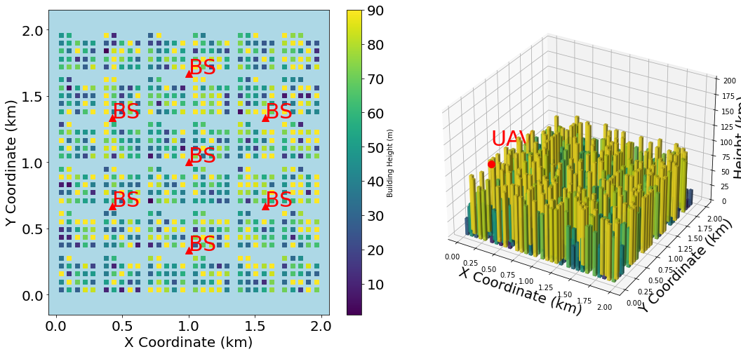
(a) Environment 1

(b) Environment 2

(c) Environment 3

Figure 1: Comparative Visualization of UAV Operational Environments: This figure illustrates the UAV’s navigation challenges and strategies across three environments. Graph a depicts a dense urban landscape with tall buildings; Graph b shows a sparse urban area with two scenarios: a standard mission and an emergency scenario, emphasizing the UAV’s adaptability to sudden environmental changes; Graph c shows a third, more differentiated scenario, modelling a suburban residential area and varying the distribution of base stations

We consider a singular UAV-aided cellular network. The core objectives of UAV are to navigate swiftly and efficiently toward a designated target location while ensuring seamless communication with a terrestrial cellular network. This operational versatility extends to diverse geographical regions, denoted as space of Environments $\mathcal{S}$ ($X_{1},X_{2},X_{3}$), as shown in Fig. 1, where each region presents unique building distribution and communication needs. Map distinctions between different environments include factors such as urban building type, building density, street width, base station height, and other relevant parameters.

BSs are deployed at specific locations within the urban area. Let $\mathcal{M}$ be the set of BSs. Each BS $m\in\mathcal{M}$ is characterized by its geographical location $(x_{s},y_{s})$ and height $h_{s}$ with 3 sectors $j$. The UAV embarks on its mission from a designated initial location, represented as $q_{I}\in\mathbb{R}^{3\times 1}$, which can vary for each deployment. The primary goal is to navigate the UAV to a predetermined target point, marked as $q_{F}\in\mathbb{R}^{3\times 1}$, while ensuring uninterrupted communication links with the terrestrial network during the mission, with the probability of communication outage maintained below requirement. The UAV moves at constant speed $V=V_{max}$ along a 3D trajectory of duration $T$ that can be divided into $K$ discrete segments with interval $\delta_{k}=T/K$, $k=\{1,...,K\}$. $\delta_{k}$ is chosen arbitrarily small so that within each step the large scale signal power received by the UAV remains approximately unchanged. Each segment is thus described by its discrete coordinates $\mathbf{q}(n)=(x_{n},y_{n},h_{n})$.

The channel model considers various factors, including large-scale path loss, small-scale fading, and environmental elements like terrain and buildings. Large-scale path loss represents the signal attenuation over distance and frequency. The path loss is typically classified into: LoS (Line-of-Sight) Path Loss Model: $l_{L}(d)=X_{L}\times d^{-\alpha_{L}}$. And NLoS (Non-Line-of-Sight): $l_{NL}(d)=X_{NL}\times d^{-\alpha_{NL}}$ [13]. We utilize the three-sector antenna model (downtilted to serve ground User Equipments [11]), as defined by the 3rd Generation Partnership Project (3GPP) specifications [14]. The antenna gain is a critical component of signal reception from ground BS to a UAV, which can be represented as $G_{m,j}(\theta,\phi)=A_{3GPPE}(\theta,\phi)+AF(\theta,\phi,n)$. It combines the 3GPP antenna element pattern ($A_{3GPPE}(\theta,\phi)$) and array factor ($AF(\theta,\phi,n)$ to represent beamforming effects [15].

Fading phenomena describe signal variations over time due to environmental changes, particularly UAV movement. Fading coefficients $f(t)$ represent instantaneous fading levels, while small-scale fading powers $f^{2}_{0,i}$ for both LoS and NLoS environments follow Nakagami-M fading models [13]. To compute the Signal-to-Interference-plus-Noise Ratio (SINR) at a UAV from a specific ground BS ($m$) sector ($j$), the Signal Power $P_{s}=P_{t,m}\times G_{m,j}(\theta,\phi)\times L_{path}(d)\times L_{fading}$, Interference Power $P_{i}=\sum_{i\neq m}P_{t,i}\times G_{i}(\theta_{i},\phi_{i})\times L_{path}(d_{i})\times L_{fading_{i}}$, and Noise Power $P_{n}=N_{0}\times B$ are considered. $P_{s}$ accounts for the desired signal power. $P_{i}$ aggregates interference from all other BSs, and $P_{n}$ represents noise power. The SINR is computed as $SINR_{max,m,j}=\frac{P_{s,j}}{P_{i}+P_{n}},(j\in J={1,2,3})$.
During UAV’s path, we consider an outage occurs when the SINR is less than or equal to $\varphi_{\text{th}}$, leading to an outage events: $\beta(\mathbf{q}(n))=1$ if $\left(\text{SINR}(q(n))\leq\varphi_{\text{th}}\right)$. The total outage events is denoted by $\Gamma=\sum_{n=0}^{T}\beta(\mathbf{q}(n))\,$.

II-B Problem Formulation

The objective of this research is to improve the adaptability of RL models, specifically DDQN, to novel environments using CTL.

Our general goal is to ensure that the training time for a policy $\pi^{s}$ in Environment $s\in\mathcal{S}$ is significantly less than the time required to train a new model from scratch for each new environment. We can thus formulate

$$\mathcal{P}:\min \quad T_{\text{train}}(\pi^{s})$$ (1a)

s.t. $$\pi_{\text{new}}^{(0)}=\pi_{\text{pre-trained}},$$ (1b)

where denoted by $T_{\text{train}}(\pi^{s})$ is the training time of policy $\pi^{s}$ in the new enviroment $s$ and (1b) specifies that a policy $\pi^{1}$ pre-trained in Environment 1 $\in\mathcal{S}$ is used as benchmark for the UAV trajectory in the new environment. Policy $\pi^{1}$ is trained using a DDQN model and then utilized for transfer learning across two additional maps or scenarios. This approach necessitates that after the transfer, the model maintains its original trajectory objectives, i.e., minimizing the steps $n$ needed to reach its destination and to keep the frequency of outage events $\Gamma$ below a certain threshold $\hat{\Gamma}$. Policy $\pi^{1}$ is thus trained to solve problem:

$$\vspace{-0.1in}\min_{n,q(n)} \quad n+K\times\Gamma$$ (2)

s.t. $$\mathbf{q}(0)=q_{I},\quad\mathbf{q}(T)=q_{F}$$ (3)

$$\Gamma<\hat{\Gamma}$$ (4)

$$h(\text{u})>h_{\text{B}}$$ (5)

$$n\leq N.$$ (6)

The variable $q(n)$ represents the UAV’s position at step $n$, $q_{I}$ and $q_{F}$ signify the initial and final positions of the UAV, while q(T) presents the target position. Constraint (4) ensures that the maximum outage events throughout the flight remain below the specified threshold. Here $h(\text{u})$ denotes the altitude of the UAV, $h_{\text{B}}$ represents the highest altitude of the building, and $N$ signifies the maximum permissible movement step of the UAV, considering battery constraints.

III RL and Continuous Learning for UAV Trajectory Design

III-A Preliminaries

DQN and its enhancement, Double DQN, represent significant advancements in integrating reinforcement learning with deep neural networks for autonomous decision-making. DQN facilitates learning from complex sensory inputs, overcoming challenges like instability and convergence issues through techniques such as experience replay and fixed Q-targets. DDQN further refines this by correcting DQN’s overestimation of Q-values, ensuring more stable and accurate outcomes. This progression makes DQN and DDQN highly effective for UAV trajectory optimization in diverse urban environments, improving navigation precision in complex scenarios.

TL further enhances the learning process by utilizing knowledge acquired in one task to expedite learning in related but distinct tasks. It operates on the principle of reusing a pre-trained model as a starting point for new tasks, significantly cutting down on the time and data needed for training in new environments or missions. Continuous Learning complements these methodologies by enabling UAVs to continually assimilate new information without discarding previously learned knowledge. This is crucial for operating in dynamic environments where conditions and obstacles may change unpredictably. Continuous learning ensures that UAVs can iteratively update their navigation strategies, maintaining peak performance and adaptability over time.

III-B DQN and DDQN for UAV Trajectory Design

In our considered scenario, the UAV navigation task is modeled in a 3D space, where the UAV must reach a target position, starting at a random position within the set range. Given our UAV trajectory optimization, we can formulate the problem as an Markov Decision Process (MDP), which is defined by a tuple $(\mathcal{S},\mathcal{A},\mathcal{P},\mathcal{R},\gamma)$. Each state $s$ represents the UAV’s current position, communication conditions, and the environment. Formally:

$$s=\{q(n),\text{SINR}(q(n))\},$$

where $q(n)$ and $\text{SINR}(q(n))$ are the UAV’s position and signal quality, respectively. The action space comprises potential directions in which the UAV can move at any given time:

$$\mathcal{A}=\{\text{move\_f},\text{move\_b},\text{move\_l},\text{move\_r}\}.$$

Given a state $s$ and an action $a$, $\mathcal{P}(s^{\prime}|s,a)$ represents the probability of transitioning to state $s^{\prime}$. Since the UAV’s movement is deterministic, given its current state and action, it will deterministically arrive at the next state. The reward function captures the objectives of minimizing the completion time and maintaining satisfactory communication. It is presented as

$$\mathcal{R}_{1}(s,a,s^{\prime})=-k1\times d(s,s_{\text{target}})-k2\times F(q_{n})-R_{\text{n}}+R_{\text{arrive}}\vspace{-0.in}$$ (7)

where k1 and k2 are weighting factors to prioritize moving closer to the destination and penalize outage events during the transition. $d(s,s_{\text{target}})$ represents the distance between the UAV’s current position and the target position. $F(q_{n})$ denotes the signal outage penalty function, which increases the loss for navigating through areas with poor signal quality. $R_{\text{n}}$ is the step penalty, and $R_{\text{arrive}}$ is the reward for reaching the target. The discount factor $\gamma$ determines the present value of future rewards. Given the MDP framework for the UAV trajectory optimization, our goal is to find a policy $\pi^{*}$ that maximizing an expected cumulative reward:

$$\pi^{*}=\arg\max_{\pi}\mathbb{E}\left[\sum_{t=0}^{T}\gamma^{t}\mathcal{R}(s_{t},a_{t},s_{t+1})\right],$$ (8)

where $\mathbb{E}$ denotes the expectation. The DQL agent uses two neural networks: a primary network for action selection and a target network for stable learning. Both DQN and DDQN utilize a similar network structure for action selection and evaluation, but DDQN’s critical distinction lies in its action evaluation mechanism, which separates action selection from its value estimation. This separation ensures a more conservative and accurate assessment of the potential of each action, thereby enhancing the performance of trajectory design. In addition to this, we have designed MDP that is more compatible with our scenarios to improve performance. This includes adding SINR information to the state to ensures that the models for transfer have sufficient depth of learning and understanding of the environment. The rewards will also be fine-tuned according to the situation when migrating to a new environment.

III-C Continuous Learning for UAV Trajectory Design

III-C1 Environments

We define the first environment that was used to train the DDQN base model as a dense urban area, characterized by a high concentration of tall buildings that demand complex navigational strategies to maintain connectivity and avoid obstacles. Transitioning to the second environment, the UAV encounters a sparse urban landscape with shorter buildings, a stark contrast to the first. This environment is explored under two distinct scenarios which are a standard mission mirroring the parameters of the dense urban environment, and an emergency scenario necessitating a sudden change in mission objectives due to a BS failure. The adaptability of the UAV is further tested in the third environment, a residential area with low housing blocks and a different BS distribution, presenting new navigational challenges and testing the UAV’s ability to generalize its learned strategies to markedly different landscapes.

III-C2 Training in different Domain

Algorithm 1 CTL with DDQN across Environments

1:Initialize DDQN in Environment 1: learning rate $\alpha_{1}$, exploration $\epsilon_{1}$, and exploration decay $\epsilon_{\text{decay},1}$.

2:Train the model with a replay buffer and a periodically updated target network to stabilize updates.

3:Save the model weights $\xi_{\text{Env1}}$ and policy $\pi_{\text{Env1}}$

4:Transfer to Env2:

5:Initialize Env2 with DDQN model weights $\xi_{\text{Env2}}\leftarrow\xi_{\text{Env1}}$ and policy $\pi_{\text{Env2}}\leftarrow\pi_{\text{Env1}}$

6:Adjust learning parameters for Env2: set new learning rate $\alpha_{2}$, $\epsilon_{2}$, and $\epsilon_{\text{decay},2}$

7:Apply the new reward function ${R}_{2}$(optional).

8:Retrain transferred model in Env2 using the fixed parameters, maintaining the strategy of experience replay and target network updates.

9:Save the updated model weights $\xi_{\text{Env2}}$ and policy $\pi_{\text{Env2}}$

10:Transfer to Env3 with process above

11:Continue this process for any subsequent environments, transferring weights and policy while adjusting learning parameters as needed

The TL process begins with training a DDQN model in a dense urban setting, streamlining the training approach to enhance efficiency without requiring full model convergence. A targeted termination criterion focuses on achieving a high success rate at the destination rather than optimizing the total reward, shortening training by 600-800 episodes. This method is chosen because, after reaching success rate convergence, the agent’s main improvements involve strategies to avoid outage events, which may vary in effectiveness across different environments. This efficient training strategy reduces overall duration and improves the model’s suitability for CTL. Subsequent findings affirm the benefits of this balanced approach, demonstrating its practical success.

This pre-trained model is then transferred to accommodate sparse urban and residential areas. This process entails transferring the learned model weights and adjusting learning parameters, including the learning rate and exploration rates, to suit each new environment’s specific characteristics (algorithm 1). Through this methodical adaptation, the UAV demonstrates not only enhanced learning efficiency but also improved performance and adaptability across diverse operational environments. By leveraging the knowledge gained in each successive environment, CTL enables the UAV to rapidly adjust to new challenges. The objective in the new environment remains aligned with our dual goals. The model, now starting with policy $\pi_{\text{new}}^{(0)}$, is further trained to adapt to the new conditions. The fine-tuning process involves iterative updates of the policy parameters:

$$\vspace{-0.3in}\pi_{\text{new}}^{(0)} =\pi_{\text{pre-trained}},$$ (9)

$$\pi_{\text{new}}^{(k+1)} =\pi_{\text{new}}^{(k)}-\alpha\cdot\nabla_{\pi_{\text{new}}}\mathcal{L}(\pi_{\text{new}}^{(k)})$$ (10)

where $\alpha$ is the learning rate, and $\mathcal{L}$ represents the loss function tailored to the new environment.

Then we evaluate the performance of the transferred model in the new environment using metrics such as convergence time $T_{\text{convergence}}$ and improvements in stability or accuracy. These metrics will demonstrate the effectiveness of TL in reducing training time and enhancing model performance in diverse urban scenarios.

TABLE I: Summary of Model Parameters

Parameter Name	Symbol	Value
Learning Rate(DDQN)	$\alpha$	0.001
Initial Exploration Rate(DDQN)	$\epsilon$	1.0
Exploration Decay Rate(DDQN)	$\epsilon_{\text{decay}}$	0.998
Learning Rate (Transfer)	$\alpha_{\text{transfer}}$	0.0002
Initial Exploration Rate (Transfer)	$\epsilon_{\text{transfer}}$	0.5
Exploration Decay Rate (Transfer)	$\epsilon_{\text{decay, transfer}}$	0.995
Arrive Target for Env1	$q_{F}1$	1000,900
Arrive Target for Env2	$q_{F}2$	1250,1300
Discount Factor	$\gamma$	0.95
Weighting Factor for Distance length	$k_{1}$	0.8
Weighting Factor for Outage Penalty	$k_{2}$	1
Step Penalty	$R_{n}$	1
Reward for Reaching Target	$R_{\text{arrive}}$	2000
Max steps per eposode	steps	200
SINR Threshold for outage	$\varphi_{\text{th}}$	0 dB
UAV Height	$h(\text{u})$	90 m

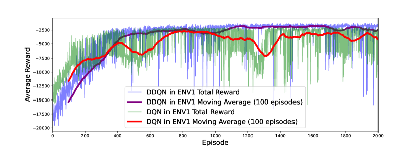
Figure 2: Compare of DQN with DDQN for Trajectory Design in Env1

IV Results

The height of the BS on the horizontal plane ranges from 5 to 25 meters, reflecting typical real-world configurations. The operational area for all maps is set to a size of $2\,\text{km}\times 2\,\text{km}$ with a height limit of 100 meters. The maximum number of steps per episode, representing the battery limitation, is set to 200 steps, with each step corresponding to a displacement of 10 meters. A UAV arriving within a 30 meters radius of the target is considered to have successfully reached its destination. The networks consist of 3 hidden layers with 64 units each, using ReLU activation functions. The output layer has linear activation corresponding to action values. The learning rate in (9) was reduced to 0.0002 for fine-tuning, allowing for more subtle weight adjustments in the later layers, thereby refining the model’s policy without drastic deviations from its pre-learned behaviors. Weighting factors for rewards (7) and more training parameters can be found in Table I.

The agent’s performance improved over time, as indicated by an increase in total reward and a decrease in the number of steps required to reach the target. The learning progress was captured through two plots: total rewards, success rate over episodes, and average level of communication. To demonstrate this, we compared how well DQN and DDQN adapted to our scenarios, choosing the one that performed better as our base model for continuous learning.

In Fig. 2 we illustrate the comparative performance between the DQN and DDQN models within the initial environment. The DQN model exhibits greater volatility throughout the training phase, with a 10-15% lower peak in average rewards for the optimum policy compared to the DDQN. Additionally, the DQN demonstrates less stable convergence by the 2000 episode, accompanied by increased variability. Thus, the DDQN model emerges as a more suitable foundational model for TL.

IV-A CTL in environment 2 with multi scenarios

This section shows the outcomes of TL in the second environment, encompassing two scenarios. Scenario one, illustrated in Fig. 3, involves utilizing the DDQN model from the first environment as the foundational model and has the same mission destinations as DDQN. The result in Fig.4 shows a more challenging scenario, which has different target positions and one of the BS is not working.

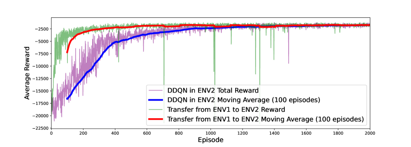
(a) Average rewards against episodes

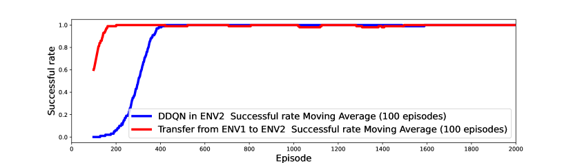
(b) Success rate against episodes

Figure 3: TL from ENV1 to ENV2 against retraining DDQN in ENV2

Fig.3(a) demonstrates the role of TL by showing the average rewards of the training, showcasing an earlier and more stable convergence compared to the DDQN model trained from scratch. The duration to achieve stable optimal rewards is shortened by 600–700 episodes, underscoring the efficiency of TL in accelerating performance and stability. The success rate of reaching the destination during training also notably underscores the efficiency of TL. As shown in Fig.3(b), the success rate stabilizes at least 99% over 250 episodes sooner than the scratch-trained model, which means that the model prioritizes finding the policy that reaches the destination and then adapts the relevant policy for the communication much faster, and this process for DDQN is much slower.

In navigating the challenges of training in a environment where a base station BS was no longer functional and the target position was further away, the UAV demonstrated commendable adaptability. Fig.4(a) illustrates the average rewards of TL, and Fig.4(b) shows the success rate in Environment 2 where, despite facing significant challenges, TL demonstrates its effectiveness by converging 300 episodes earlier in terms of average reward and 200 episodes earlier in reaching the target than the model trained from scratch. This scenario limited the CTL approach from fully exploiting all initial strategies as compared to a model beginning from scratch. It shows slight fluctuations during the training phase, these did not hinder the overall process convergence, which showcases the robustness of the UAV’s learning capabilities. The observed variations, partly due to the task’s target location moving further away, marginally slowed the learning speed but did not detract from the UAV’s ability to readjust and progress. Therefore, the performance of CTL is expected and acceptable when faced with more challenging scenarios and altered tasks. The CTL efficiently navigated these complexities, underlining the effectiveness of its adaptive learning framework in dynamic environments.

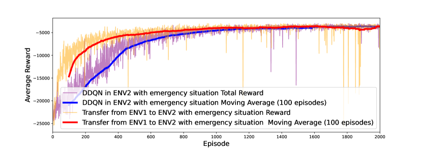
(a) Average rewards against episodes

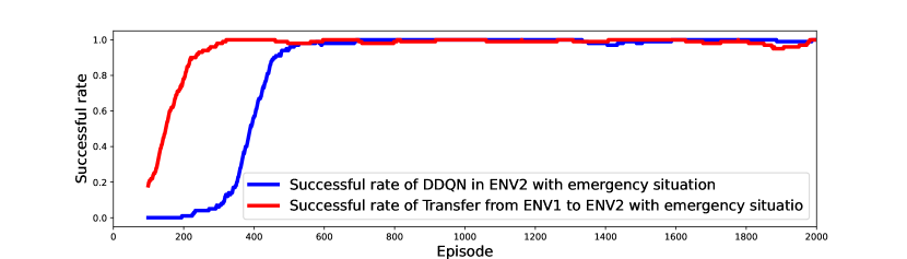
(b) Success rate against episodes

Figure 4: TL from ENV1 to ENV2 with emergency scenario against retraining DDQN in ENV2

IV-B CTL in environment 3 more differences

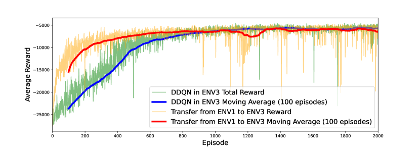
(a) Average rewards against episodes

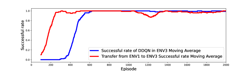
(b) Success rate against episodes

Figure 5: TL from ENV1 to ENV3 against retraining DDQN in ENV3

In the third environment (Fig.5), the role is to test the potential for CTL. We designed the third environment to be very different from the environment used for the base model. This includes the distribution of buildings, height, size, number of BS locations, and changes in the target destination. The CTL still demonstrates strong capabilities; the convergence was 200 episodes faster and reached a stable success rate 150 episodes earlier. However, more fluctuations were encountered later on, which is predictable for reasons similar to those discussed in Environment 2, as not all environments were explored completely. This serves as an effective illustration of the capabilities of continuous learning to expedite model training outcomes, even when faced with environments that present significant disparities.

V Conclusion

In conclusion, the performance of CTL across two distinct environments demonstrated its effectiveness in accelerating learning and achieving higher success rates compared to training DDQN models from scratch. For transfer to similar environments, TL showcased a notable advantage in terms of stability and early convergence, with the second case highlighting its capacity to adapt to more complex tasks and scenarios, albeit with reduced efficiency and some late-stage fluctuations. The third environment, significantly divergent from the initial training context, further tested the limits of CTL, where, despite faster convergence and commendable performance, the model faced increased fluctuations due to incomplete exploration of the new environment. These findings underscore the potential of TL to enhance model adaptability and efficiency, particularly in dynamically changing or progressively complex scenarios, while also pointing to the need for strategies to mitigate late-stage performance variability. In our future works we plan to investigate this issue and work on strategies that deal with this performance variability, and more in-depth study of energy conservation strategies.

5G

Fifth Generation

6G

Sixth Generation

AI

Artificial Intelligent

ACO

Ant Colony Optimization

ANN

Artificial Neural Network

BB

Base Band

BBU

Base Band Unit

BER

Bit Error Rate

BS

Base Station

BW

bandwidth

C-RAN

Cloud Radio Access Networks

CU

Central Unit

RU

Radio Unit

DU

Distributed Unit

CAPEX

Capital Expenditure

CoMP

Coordinated Multipoint

CR

Cognitive Radio

CRLB

Cramer-Rao Lower Bound

C-RAN

Cloud Radio Access Network

CTL

Continuous Transfer Learning

D2D

Device-to-Device

DAC

Digital-to-Analog Converter

DAS

Distributed Antenna Systems

DBA

Dynamic Bandwidth Allocation

PID

Proportional–integral–derivative

DC

Duty Cycle

DFRC

Dual Function Radar Communication

DL

Deep Learning

DSA

Dynamic Spectrum Access

DQL

Deep Q Learning

DRL

Deep Reinforcement Learning

DQN

Deep Q-Network

DDQN

double deep Q network

DDPG

Deep Deterministic Policy Gradient

FBMC

Filterbank Multicarrier

FEC

Forward Error Correction

FFR

Fractional Frequency Reuse

FL

Federated Learning

FSO

Free Space Optics

FANET

Flying ad-hoc network

GA

Genetic Algorithms

GAN

Generative Adversarial Networks

GMMs

Gaussian mixture models

HAP

High Altitude Platform

HL

Higher Layer

HARQ

Hybrid-Automatic Repeat Request

HCA

Hierarchical Cluster Analysis

HO

Handover

KNN

k-nearest neighbors

IoT

Internet of Things

ISAC

Integrated Sensing and Communication

LAN

Local Area Network

LAP

Low Altitude Platform

LL

Lower Layer

LoS

Line of Sight

LTE

Long Term Evolution

LTE-A

Long Term Evolution Advanced

MAC

Medium Access Control

MAP

Medium Altitude Platform

MDP

Markov Decision Process

ML

Machine Learning

MME

Mobility Management Entity

mmWave

millimeter Wave

MIMO

Multiple Input Multiple Output

NFP

Network Flying Platform

NFPs

Network Flying Platforms

NLoS

Non-Line of Sight

RU

Radio Unit

OFDM

Orthogonal Frequency Division Multiplexing

OSA

Opportunistic Spectrum Access

O-RAN

Open Radio Access Network

C-RAN

cloud radio access network

OMC

O-RAN Management and Control

PAM

Pulse Amplitude Modulation

PAPR

Peak-to-Average Power Ratio

PGW

Packet Gateway

PHY

physical layer

PSO

Particle Swarm Optimization

PU

Primary User

QAM

Quadrature Amplitude Modulation

QoE

Quality of Experience

QoS

Quality of Service

QPSK

Quadrature Phase Shift Keying

RF

Radio Frequency

RIS

Reconfigurable Intelligent Surface

RL

Reinforcement Learning

DRL

Deep Reinforcement Learning

RMSE

Root Mean Squared Error

RN

Remote Node

RRH

Remote Radio Head

RRC

Radio Resource Control

RRU

Remote Radio Unit

RSS

Received Signal Strength

SAR

synthetic-aperture radar

SU

Secondary User

SCBS

Small Cell Base Station

SDN

Software Defined Network

SNR

Signal-to-Noise Ratio

SON

Self-organising Network

SVM

Support Vector Machine

TDD

Time Division Duplex

TD-LTE

Time Division LTE

TDM

Time Division Multiplexing

TDMA

Time Division Multiple Access

TL

Transfer Learning

UE

User Equipment

ULA

Uniform Linear Array

UAV

Unmanned Aerial Vehicle

USRP

Universal Software Radio Platform

XAI

Explainable AI

HCP

heterogeneous computing platform

IoT

Internet of Things

References

- [1] J. Won, D.-Y. Kim, Y.-I. Park, and J.-W. Lee, “A survey on UAV placement and trajectory optimization in communication networks: From the perspective of air-to-ground channel models,” ICT Express, 2022.
- [2] P. S. Bithas, E. T. Michailidis, N. Nomikos, D. Vouyioukas, and A. G. Kanatas, “A survey on machine-learning techniques for UAV-based communications,” Sensors, vol. 19, no. 23, p. 5170, 2019.
- [3] C. Sun, G. Fontanesi, B. Canberk, A. Mohajerzadeh, S. Chatzinotas, D. Graces, and H. Ahmadi, “Advancing uav communications: A comprehensive survey of cutting-edge machine learning techniques,” IEEE Open Journal of Vehicular Technology, pp. 1–31, 2024.
- [4] S. Yin, S. Zhao, Y. Zhao, and F. R. Yu, “Intelligent trajectory design in UAV-aided communications with reinforcement learning,” IEEE Transactions on Vehicular Technology, vol. 68, no. 8, pp. 8227–8231, 2019.
- [5] J. Moon, S. Papaioannou, C. Laoudias, P. Kolios, and S. Kim, “Deep reinforcement learning multi-UAV trajectory control for target tracking,” IEEE Internet of Things Journal, vol. 8, no. 20, pp. 15 441–15 455, 2021.
- [6] B. Zhu, E. Bedeer, H. H. Nguyen, R. Barton, and J. Henry, “UAV trajectory planning in wireless sensor networks for energy consumption minimization by deep reinforcement learning,” IEEE Transactions on Vehicular Technology, vol. 70, no. 9, pp. 9540–9554, 2021.
- [7] R. Ding, F. Gao, and X. S. Shen, “3D UAV trajectory design and frequency band allocation for energy-efficient and fair communication: A deep reinforcement learning approach,” IEEE Transactions on Wireless Communications, vol. 19, no. 12, pp. 7796–7809, 2020.
- [8] G. Fontanesi, A. Zhu, and H. Ahmadi, “Deep reinforcement learning for dynamic band switch in cellular-connected uav,” in 2021 IEEE 94th Vehicular Technology Conference (VTC2021-Fall), 2021, pp. 1–5.
- [9] H. Yang, J. Zhang, S. Song, and K. B. Lataief, “Connectivity-aware uav path planning with aerial coverage maps,” in 2019 IEEE Wireless Communications and Networking Conference (WCNC). IEEE, 2019, pp. 1–6.
- [10] Z. Chen, X. Liang, and M. Zheng, “Knowledge transfer between different UAVs for trajectory tracking,” IEEE Robotics and Automation Letters, vol. 5, no. 3, pp. 4939–4946, 2020.
- [11] G. Fontanesi, A. Zhu, M. Arvaneh, and H. Ahmadi, “A transfer learning approach for UAV path design with connectivity outage constraint,” IEEE Internet of Things Journal, vol. 10, no. 6, pp. 4998–5012, 2022.
- [12] X. Zhang, G. Zheng, and S. Lambotharan, “Trajectory design for UAV-assisted emergency communications: A transfer learning approach,” in GLOBECOM 2020-2020 IEEE Global Communications Conference. IEEE, 2020, pp. 1–6.
- [13] G. Fontanesi, A. Zhu, and H. Ahmadi, “Outage analysis for millimeter-wave fronthaul link of UAV-aided wireless networks,” IEEE Access, vol. 8, pp. 111 693–111 706, 2020.
- [14] B. Mondal, T. A. Thomas, E. Visotsky, F. W. Vook, A. Ghosh, Y.-H. Nam, Y. Li, J. Zhang, M. Zhang, Q. Luo et al., “3D channel model in 3GPP,” IEEE Communications Magazine, vol. 53, no. 3, pp. 16–23, 2015.
- [15] M. Rebato, L. Resteghini, C. Mazzucco, and M. Zorzi, “Study of realistic antenna patterns in 5G mmwave cellular scenarios,” in 2018 IEEE International Conference on Communications (ICC). IEEE, 2018, pp. 1–6.