A finite-sample generalization bound for stable LPV systems

Dániel Rácz1, Martin Gonzalez2, Mihály Petreczky3, András Benczúr4 and Bálint Daróczy4 This research was supported by the European Union project RRF-2.3.1-21-2022-00004 within the framework of the Artificial Intelligence National Laboratory, by the C.N.R.S. E.A.I. project ”StabLearnDyn” and by the E.D.F. project 101103386 ”FaRADAI”. 1HUN-REN SZTAKI and ELTE, Budapest, Hungary racz.daniel@sztaki.hun-ren.hu2Institut de Recherche Technologique SystemX, Palaiseau, France3 Univ. Lille, CNRS, Centrale Lille, UMR 9189 CRIStAL, F-59000 Lille, France4HUN-REN SZTAKI, Budapest, Hungary
Abstract

One of the main theoretical challenges in learning dynamical systems from data is providing upper bounds on the generalization error, that is, the difference between the expected prediction error and the empirical prediction error measured on some finite sample. In machine learning, a popular class of such bounds are the so-called Probably Approximately Correct (PAC) bounds. In this paper, we derive a PAC bound for stable continuous-time linear parameter-varying (LPV) systems. Our bound depends on the $H_{2}$ norm of the chosen class of the LPV systems, but does not depend on the time interval for which the signals are considered.

I Introduction

LPV [1] systems are a popular class of dynamical systems control and system identification, e.g. ([2, 3, 4, 5, 1, 6, 7, 8]). Generally, LPV systems are linear in state, input and output signals, but the coefficients of these linear relationships depend on the scheduling variables. These systems are popular due to their ability to model highly non-linear phenomena while allowing much simpler theoretical analysis. In this work, we consider continuous-time LPV systems in state-space form, where the system matrices are affine functions of the scheduling variables.

Contribution. In learning and parametric system identification our starting point is a parametrized family of LPV systems, and our goal is to find a member of this family, which predicts as accurately as possible the true output for each input and scheduling variable. To this end, we assume that we have a dataset consisting triplets of signals representing the input, the scheduling signal and the corresponding output of the true system, all defined on the finite time interval $[0,T]$, and measured during the learning/identification experiment. Learning/system identification algorithms then choose a concrete element of the parameterized family of LPV systems, which predicts the best outputs from this dataset used for learning. However, for the identified model to be useful, especially for control, it should accurately predict the true output for inputs and scheduling signals which were not used during identification, i.e., it should generalize well. A widespread measure of generalization is the true loss, i.e. the expected value of the prediction error, if the inputs and scheduling signals are sampled from the same distribution as in the dataset used for learning. Unfortunately, the true loss is unknown in general, but it can be approximated by the empirical loss, i.e. the average of prediction errors by a certain model, where the average is taken over the elements of the data set.

It is well-known that the empirical loss converges to the true loss as the number of data points grow, e.g., [9, Lemma 8.2]. However, for the purposes of evaluating the true loss based on the empirical loss, it is of interest to have a uniform bound, with respect to the parameterized family, on the difference between the true loss and the empirical loss. Such uniform bounds are referred to as PAC bounds in the literature [10, 11], and they are a standard tool for theoretical analysis of statistical learning algorithms.

In this paper, we derive a particular PAC bound for LPV systems. The derived bound is of the magnitude $O(c/\sqrt{N})$, where $c$ is a constant that depends on the parametrization, and $N$ is the cardinality of an arbitrary finite sample used to evaluate or identify the model. The constant $c$ is the maximal $H_{2}$ norm of the elements of the parametrization. In contrast to related results, the constant $c$, and thus the bound, does not depend on the length of the time interval $[0,T]$.

Using PAC bounds for learning. PAC bounds can be used in several ways [10, 11], without claiming completeness, we mention the following applications: (1) to evaluate the performance of identified models based on their performance on a dataset (the training or the validation set), (2) to analyze the effect of various quantities appearing in the bound (norms, VC-dimension, number of data points) on the generalization capability of the learned models, in particular, characterizing the amount of data necessary for learning adequate models, (3) to select parametrizations which minimize the PAC bound and hence are more likely to allow learning models which generalize well and avoid overfitting.

Motivation: system identification. PAC bounds are expected to have the same applications for system identification as for learning, i.e. they will enable a sharper theoretical analysis of system identification algorithms, by making explicit relationship between the empirical and true losses as functions of the number of data points and various properties of the parametrization.

Motivation: Machine Learning. There is consensus in the machine learning community on the usefulness of PAC bounds. Continuous-time dynamical systems, e.g. continuous-time Recurrent Neural Networks (RNNs, [12]), Neural Controlled Ordinary Differential Equations (NCDEs, [13]) or structured State-Space Models (SSMs, [14]) are becoming increasingly popular in machine learning. Since LPV systems include bilinear systems [15] as a special case, in principle they could be used as universal approximators for sufficiently smooth dynamical systems [16], including important subclasses of RNNs and NCDEs. Finally, LPV systems include linear state-space models, which are crucial ingredients of SSMs, and subclasses of RNNs, hence PAC bounds for LPV systems are expected to be useful for PAC bounds for NCDEs, RNNs and SSMs.

Related work. PAC bounds for discrete-time linear systems were explored in system identification in [17, 18], but not for LPV systems in state-space form and continuous-time. There are several PAC bounds available for continuous-time RNNs and nonlinear systems [19, 20, 21, 22, 23, 24], but these are exponential in the integration time. The literature on finite-sample bounds for learning discrete-time dynamical systems, e.g. [17, 25, 26, 27], considers different learning problems.

Significance and novelty. The main novelty is that (1) our error bound does not depend on the length of the integration interval $T$, (2) it exploits quadratic stability, (3) it uses $H_{2}$ norm defined via Volterra-kernels to estimate the Rademacher complexity. This is in contrast [24, 19, 22, 23] which used Fliess-series expansions for that purpose. It was precisely the use of Volterra-series and $H_{2}$ norms which allowed us to formulate bounds which do not grow with $T$. In turn, the latter is important as dynamical systems are often used for making long-term predictions.

Structure of the paper. Next, in Section II we set notations and definitions related to the LPV system, then in Section III we define the problem of generalization in case of LPV systems, when we can only measure the error of the system on a finite set of sequences. In our case this set is a particular set of LPV systems, which meet the stability and other crucial conditions for having a time-invariant bound. We define these conditions and the $H_{2}$ norm of output in Section IV. We state our time-independent bound in Section V for the generalization gap, the difference between the true error and the error measured on the finite set of sequences, based on the Rademacher complexity of the hypothesis set. We prove our bound in Section VI by showing that under our assumptions the LPV system has finite $H_{2}$ norm, thus we may upper bound the Rademacher complexity of the system. Finally, in Section VII we consider a system and a dataset, we estimate the elements of the bound and show that the bound in this case is meaningful.

II LPV systems

In this paper, we consider LPV state-space representations with affine dependence on the parameters (LPV-SSA), i.e. systems of the form

$$\Sigma\begin{cases}\dot{x}(t)=A(p(t))x(t)+B(p(t))u(t),~{}x(0)=0\\ y_{\Sigma}(t)=C(p(t))x(t)\\ \end{cases}$$ (1)

where $x(t)\in\mathbb{R}^{n_{\text{x}}}$ is the state vector, $u(t)\in\mathbb{R}^{n_{\text{in}}}$ is the input and $y_{\Sigma}(t)\in\mathbb{R}^{n_{\text{out}}}$ is the output of the system for all $t\in[0,T]$, and $n_{\text{x}},n_{\text{in}},n_{\text{out}}\in\mathbb{N}^{+}$. The vector $p(t)=(p_{1}(t),\dots,p_{n_{\text{p}}}(t))^{T}\in\mathbb{P}\subseteq\mathbb{R}^{n_{\text{p}}}$ is the scheduling variable for $n_{\text{p}}\in\mathbb{N}^{+}$. Note that $n_{p}$ is the number of scheduling variables in the system, therefore it is the most important parameter regarding the complexity of the system. The matrices of the system $\Sigma$ are assumed to depend on $p(t)$ affinely, i.e. $A(p(t))=A_{0}+\sum\limits_{i=1}^{n_{\text{p}}}p_{i}(t)A_{i}$, $B(p(t))=B_{0}+\sum\limits_{i=1}^{n_{\text{p}}}p_{i}(t)B_{i}$ and $C(p(t))=C_{0}+\sum\limits_{i=1}^{n_{\text{p}}}p_{i}(t)C_{i}$ for matrices $A_{i}\in\mathbb{R}^{n_{\text{x}}\times n_{\text{x}}},B_{i}\in\mathbb{R}^{n_{\text{x}}\times n_{\text{in}}}$ and $C_{i}\in\mathbb{R}^{n_{\text{out}}\times n_{\text{x}}}$, $i=0,\ldots,n_{\text{p}}$, which do not depend on time or the scheduling signal. We identify the LPV-SSA $\Sigma$ with the tuple $\Sigma=(A_{i},B_{i},C_{i})_{i=0}^{n_{\text{p}}}$.

A solution of $\Sigma$ refers to the tuple of functions $(u,p,x,y_{\Sigma})$, all defined on $[0,T]$, such that $x$ is absolutely continuous, $y_{\Sigma}$, $u$ and $p$ are piecewise continuous and they satisfy (1). Note that the output $y_{\Sigma}$ is uniquely determined by $u$ and $p$, since the initial state $x(0)$ is set to zero. To emphasize this dependence, we denote $y_{\Sigma}$ by $y_{\Sigma}(u,p)$. Thus, the scheduling signal $p(t)$ behaves as an external input, too.

For the sake of compactness we make a series of simplifications. First, as already stated, the initial state is set to zero. This is not a real restriction, as we consider stable systems for which the contribution of the non-zero initial state decays exponentially. Second, we work with systems with scalar output, i.e. let $n_{\text{out}}=1$. Third, we assume that the scheduling variables take values in $\mathbb{P}\subseteq[-1,1]^{n_{\text{p}}}$. This is a standard assumption in the literature [1] and it can always be achieved by an affine transformation, if the scheduling variables take values in a suitable interval.

III Learning problem and generalization

We now define the learning problem for LPV systems along the lines of classical statistical learning theory [11]. For this purpose, let us fix a time interval $[0,T]$ and a set $\mathcal{E}$ of LPV systems of the form (1).

Let $\mathcal{U}$, $\mathcal{P}$ and $\mathcal{Y}$ be sets of piecewise continuous functions defined on $[0,T]$ and taking values in $\mathbb{R}^{n_{\text{in}}}$, $\mathbb{P}$ and $\mathbb{R}^{n_{\text{out}}}$ respectively. Hereinafter we use the standard terminology of probability theory [28]. Consider the probability space $(\mathcal{U}\times\mathcal{P}\times\mathcal{Y},\mathcal{B},\mathcal{D})$, where $\mathcal{B}$ is a suitable $\sigma$-algebra and $\mathcal{D}$ is a probability measure on $\mathcal{B}$. For example, $\mathcal{B}$ could be the direct product of the standard cylindrical Borel $\sigma$-algebras defined on the function spaces $\mathcal{U},\mathcal{P}$ and $\mathcal{Y}$. Let us denote by $\mathcal{D}^{N}$ the $N$-fold product measure of $\mathcal{D}$ with itself. We use $E_{(u,p,y)\sim\mathcal{D}}$, $P_{(u,p,y)\sim\mathcal{D}}$, $E_{S\sim\mathcal{D}^{N}}$ and $P_{S\sim\mathcal{D}^{N}}$ to denote expectations and probabilities w.r.t. the measures $\mathcal{D}$ and $\mathcal{D}^{N}$ respectively. The notation $S\sim\mathcal{D}^{N}$ tacitly assumes that $S\in(\mathcal{U}\times\mathcal{P}\times\mathcal{Y})^{N}$, i.e. $S$ is made of $N$ triplets of input, scheduling and output trajectories. Intuitively, we think of $S$ as a dataset of size N drawn randomly and independently from the distribution $\mathcal{D}$.

Consider a loss function $\ell:\mathbb{R}\times\mathbb{R}\rightarrow[0,+\infty)$, which measures the discrepancy between two possible output values. Some of the widespread choices are $\ell(a,b)=\|a-b\|$ or $\ell(a,b)=\|a-b\|^{2}$.

The learning objective is to find an LPV system $\Sigma\in\mathcal{E}$ such that the true risk at time $T$, defined as

$\displaystyle\mathcal{L}(\Sigma)=\mathbb{E}_{(u,p,y)\sim\mathcal{D}}[\ell(y_{\Sigma}(u,p)(T),y(T))]$

is as small as possible. Since the distribution $\mathcal{D}$ is unknown, minimizing the true risk is impossible. Therefore, the true risk is approximated by the empirical risk at time $T$ w.r.t. a dataset $S=\{(u_{i},p_{i},y_{i})\}_{1\leq i\leq N}$, defined as

$\displaystyle\mathcal{L}_{N}^{S}(\Sigma)=\frac{1}{N}\sum\limits_{i=1}^{N}\ell(y_{\Sigma}(u_{i},p_{i})(T),y_{i}(T)).$

In practice, selecting an appropriate model is done by minimizing the empirical risk w.r.t. a so-called training dataset, while the trained model is usually evaluated by computing the empirical risk w.r.t. a separate test dataset. In both cases, we need a bound on the difference between the true and the empirical risk. That is, we need to bound the generalization gap, defined as $\sup_{\Sigma\in\mathcal{E}}(\mathcal{L}(\Sigma)-\mathcal{L}_{N}^{S}(\Sigma))$.

Remark III.1

In the data, the scheduling signal $p$ may depend on $u$ or $y$, and the data may be generated by a quasi-LPV system. However, for the models to be learnt the scheduling signal acts as an input, as it is customary in system identification for LPV systems [1].

IV Technical preliminaries and assumptions

We start by presenting a Volterra-series representation of the output of an LPV system of the form (1), which plays a central role in formulating and proving the main result. To this end, we introduce the following notation.

Notation (Iterated integrals). Let $\Delta_{k}^{t}=\left\{(\tau_{k},\dots,\tau_{1})\mid t\geq\tau_{k}\geq\dots\geq\tau_{1}\geq 0\right\}\subset\mathbb{R}^{k}$ for any positive integer $k$. Moreover, let $\Delta_{k}^{\infty}=\left\{(\tau_{k},\dots,\tau_{1})\mid\tau_{k}\geq\dots\geq\tau_{1}\geq 0\right\}$. Clearly, $\Delta_{k}^{t}\subseteq\Delta_{k}^{\infty}$ for all $t\in[0,+\infty)$. For $t\in\mathbb{R}$ and $\tau=(\tau_{k},\ldots,\tau_{1})$ we use the notation $(t,\tau)=(t,\tau_{k},\ldots,\tau_{1})$. In addition, we use the following notation for iterated integrals (for any function $f$ for which the integrals are well defined), for $t\in[0,+\infty]$

$\displaystyle\int_{\Delta_{k}^{t}}f(\tau)\,d\tau\equiv\int_{0}^{t}\int_{0}^{\tau_{k}}\cdots\int_{0}^{\tau_{2}}f(\tau_{k},\ldots,\tau_{1})\,d\tau_{1}\cdots\,d\tau_{k}.$

Let $[n]=\{1,\ldots,n\}$ and $[n]_{0}=\{0,\ldots,n\}$ for all $n\in\mathbb{N}$. Let $I_{k}=[n_{\text{p}}]^{k}$ be the set of multi-indices of length $k$, so an element $I$ of $I_{k}$ is a tuple of the form $I=(i_{1},\ldots,i_{k})$. By slight abuse of notation, let $I_{0}$ be the singleton set $\{\emptyset\}$. For a system $\Sigma$ of the form (1), for every $I\in I_{k}$, $t\in[0,+\infty)$, $i_{q},i_{r}\in[n_{\text{p}}]_{0}$, and for every $p\in\mathcal{P}$, $u\in\mathcal{U}$ and $\lambda\geq 0$, we define the $\lambda$-weighted LPV Volterra-kernels $w_{i_{q},i_{r},I}^{\lambda}:\Delta_{k+1}^{\infty}\rightarrow\mathbb{R}^{1\times n_{\text{in}}}$, the scheduling product $p_{I}:\Delta_{k+1}^{T}\rightarrow\mathbb{R}$ and the $\lambda$-weighted scheduling-input product $\varphi_{i_{q},i_{r},I}^{\lambda}:\Delta_{k+1}^{T}\rightarrow\mathbb{R}^{n_{\text{in}}}$ as follows. For $k=0$ and $I=\emptyset$, for any $\tau=(\tau_{1})\in\Delta_{1}^{t}=[0,t]$, set

$\displaystyle w^{\lambda}_{i_{q},i_{r},\emptyset}(\boldsymbol{\tau}):=C_{i_{q}}e^{A_{0}\tau_{1}}B_{i_{r}}e^{\frac{\lambda}{2}\tau_{1}},~{}p_{\emptyset}(\tau):=1,$
$\displaystyle\varphi_{i_{q},i_{r},\emptyset}^{\lambda}(\tau):=p_{i_{q}}(T)p_{i_{r}}(T-\tau_{1})u(T-\tau_{1})e^{-\frac{\lambda}{2}\tau_{1}}.$

For $k>0$, $\tau=(\tau_{k+1},\ldots,\tau_{1})\in\Delta_{k+1}^{t}$, $t=\infty$ or $t=T$ respectively and $I=(i_{1},\ldots,i_{k})$ set

$\displaystyle w_{i_{q},i_{r},I}^{\lambda}(\tau):=$
$\displaystyle C_{i_{q}}e^{A_{0}(\tau_{k+1}-\tau_{k})}A_{i_{k}}e^{A_{0}(\tau_{k}-\tau_{k-1})}\cdots A_{i_{1}}e^{A_{0}\tau_{1}}B_{i_{r}}e^{\frac{\lambda}{2}\tau_{k+1}},$
$\displaystyle p_{I}(\tau):=\prod_{j=1}^{k}p_{i_{j}}(\tau_{j}+T-\tau_{k+1}),$
$\displaystyle\varphi^{\lambda}_{i_{q},i_{r},I}(\tau):=p_{i_{q}}(T)p_{i_{r}}(\tau_{k+1})p_{I}(\tau)u(T-\tau_{k+1})e^{-\frac{\lambda}{2}\tau_{k+1}}.$

In the definition above, the value $k$ is always equal to the size of the tuple $I$. The respective domains of these functions each contain tuples of size $k+1$ (denoted by $\tau$). The $\lambda$-weighted LPV Volterra kernels represent weighted Volterra kernels of certain bilinear systems, outputs of which determine the output of (1). The $\lambda$-weighted scheduling-input products capture the polynomial relationship between the outputs of these bilinear systems and the scheduling and input signals. The weighting was introduced in order to make the series of the $L^{2}$ norms of these products square summable. The terms belonging to $i_{r}$ and $i_{q}$ are related to the effect of $B_{i_{r}}$ and $C_{i_{q}}$ on the output of (1). The following Lemma captures this intuition in a rigorous way.

Lemma IV.1

For every $(u,p)\in\mathcal{U}\times\mathcal{P}$, $\lambda\geq 0$, the output of $\Sigma$ at time $T$ admits the following representation:

$\displaystyle y_{\Sigma}(u,p)(T)\!\!=\!\!\sum\limits_{i_{q},i_{r}=0}^{n_{\text{p}}}\sum\limits_{k=0}^{\infty}\sum\limits_{I\in I_{k}}\int_{\Delta_{k+1}^{T}}\!\!\!\!w^{\lambda}_{i_{q},i_{r},I}(\tau)\varphi^{\lambda}_{i_{q},i_{r},I}(\boldsymbol{\tau})d\tau.$

The proof is based on a Volterra series expansion [15] and can be found in [29, Appendix A].This observation allows us to represent the output of an LPV system as a scalar product in a suitable Hilbert space which turns out to be the key for the proof of the main result.

Next, we define the $\lambda$-weighted $H_{2}$ norm, a variant of the classical $H_{2}$ norm, parameterized by a constant $\lambda>0$,

$\displaystyle\left\lVert\Sigma\right\rVert_{\lambda,H_{2}}^{2}\!\!:=$ $\displaystyle\!\!\sum_{i_{q},i_{r}=0}^{n_{\text{p}}}\sum_{k=0}^{\infty}\sum_{I\in I_{k}}\int_{\Delta_{k+1}^{\infty}}\left\lVert w_{i_{q},i_{r},I}^{\lambda}(\tau)\right\rVert_{2}^{2}d\tau.$
Remark IV.2

The norm $\left\lVert\Sigma\right\rVert_{\lambda,H_{2}}$ is finite, if the Volterra kernels $w_{i_{q},i_{r},I}^{\lambda}$ are finite energy signals and the sum of their $L_{2}$ norms is finite too. For $\lambda=0$, the definition $\left\lVert\Sigma\right\rVert_{\lambda,H_{2}}$ is a direct extension for bilinear systems [30]. When applied to LTI systems with $\lambda=0$, the above defined norm is the $H_{2}$ norm. For LPV systems there are several possible definitions of $H_{2}$ norms, which are not equivalent, not even for linear, time-varying systems, for an overview see [31, Section 2.2]. The norm $\left\lVert\Sigma\right\rVert_{\lambda,H_{2}}$ is different from these other $H_{2}$ norms for LPV systems. However, as it is shown in Lemma IV.4 below, under certain stability conditions this norm exists, and similarly to other $H_{2}$ norms, it is an upper bound on peak output under unit energy input. We use this norm instead of other $H_{2}$ norms to succesfully upper bound the Rademacher complexity in the proof of the main result.

In order to state the main result of the paper, we need to state several assumptions. To this end, we introduce the following notation. Let us denote by $L^{2}([0,T],\mathbb{R}^{n_{\text{in}}})$ the space of all measurable functions $f:[0,T]\rightarrow\mathbb{R}^{n_{\text{in}}}$ such that $\left\lVert f\right\rVert^{2}_{L^{2}([0,T],\mathbb{R}^{n_{\text{in}}})}:=\int_{0}^{T}\|f(t)\|_{2}^{2}dt$ is finite.

Assumption IV.3

Stability. There exists $\lambda\geq n_{\text{p}}$ such that for any $\Sigma\in\mathcal{E}$ of the form (1) there exists $Q\succ 0$ such that

$\displaystyle A_{0}^{T}Q+QA_{0}+\sum\limits_{i=1}^{n_{\text{p}}}A_{i}^{T}QA_{i}+\sum\limits_{i=0}^{n_{\text{p}}}C_{i}^{T}C_{i}\prec-\lambda Q.$ (2)

Bounded $H_{2}$ norm. We assume that $\sup_{\Sigma\in\mathcal{E}}\left\lVert\Sigma\right\rVert_{\lambda,H_{2}}\leq c_{\mathcal{E}}$.
Bounded signals. For any $u\in\mathcal{U}$ and $y\in\mathcal{Y}$, $\left\lVert u\right\rVert_{L^{2}([0,T],\mathbb{R}^{n_{\text{in}}})}\leq L_{u}$ and $|y(T)|\leq c_{y}$.
Lipschitz loss function. The loss function $\ell$ is $K_{\ell}$-Lipschitz-continuous, i.e. $|\ell(y_{1},y_{1}^{\prime})-\ell(y_{2},y_{2}^{\prime})|\leq K_{\ell}(|y_{1}-y_{2}|+|y_{1}^{\prime}-y_{2}^{\prime}|)$ for all $y_{1},y_{2},y_{1}^{\prime},y_{2}^{\prime}\in\mathbb{R}$, and $\ell(y,y)=0$ for all $y\in\mathbb{R}$.

Discussion on the assumptions. The first assumption ensures quadratic stability of all LPV systems in the parametrization with a decay rate $\frac{\lambda}{2}$, and it ensures the finiteness of $H_{2}$ norms:

Lemma IV.4

If (2) with $\lambda\geq n_{\text{p}}$ and $Q\succ 0$, then for any $\Sigma\in\mathcal{E}$, $\left\lVert\Sigma\right\rVert_{\lambda,H_{2}}^{2}\leq\sum_{i_{r}=0}^{n_{\text{p}}}\mathrm{trace}(B_{i_{r}}^{T}QB_{i_{r}})<+\infty.$ Additionally, for any $u\in\mathcal{U}$, $p\in\mathcal{P}$, we have

$|y_{\Sigma}(u,p)(T)|\leq(n_{\text{p}}+1)\left\lVert\Sigma\right\rVert_{\lambda,H_{2}}\left\lVert u\right\rVert_{L^{2}([0,T],\mathbb{R}^{n_{\text{in}}})}.$

The proof can be found in [29, Appendix B].

The first assumption is not restrictive as it can be translated into inequalities on the eigenvalues of the system matrices [29, Appendix B], which are not too difficult to ensure by choosing a suitable parametrization.

The second assumption is that the $\lambda$-weighted $H_{2}$ norm of the elements of class $\mathcal{E}$ are bounded by $c_{\mathcal{E}}$. This assumption holds for instance for continuous parametrizations with a bounded compact parameter set.

The third assumption means that the input signal has a finite energy and the output signal is bounded. The assumption on $|y(T)|$ means the true labels are bounded. By Lemma IV.4, the first two assumptions along with finite energy inputs already imply that the outputs of the systems from $\mathcal{E}$ are bounded uniformly by a suitable $c$. In practice, considering finite energy inputs and bounded outputs is often natural.

The last assumption is standard in machine learning, it is satisfied for $\ell(y,y^{{}^{\prime}})=$ $|y-y^{{}^{\prime}}|$, and even for the square loss, if the latter is restricted to bounded labels.

V Main result

We are ready to state our main contribution.

Theorem V.1 (Main result)

Let $c:=2K_{\ell}\max\{L_{u}(n_{\text{p}}+1)c_{\mathcal{E}},c_{y}\}$ and $R(\delta):=c\left(2+4\sqrt{2\log(4/\delta)}\right)$. Under Assumptions IV.3 , for any $\delta\in(0,1)$, we have

$\displaystyle\mathbb{P}_{\mathbf{S}\sim\mathcal{D}^{N}}\Bigg{(}\forall\Sigma\in\mathcal{E}:\mathcal{L}(\Sigma)-\mathcal{L}^{S}_{N}(\Sigma)\leq\frac{R(\delta)}{\sqrt{N}}\Bigg{)}\geq 1-\delta.$

Application of PAC to system identification. Any system identification algorithm maps a dataset $S$ to a model $\hat{\Sigma}=\hat{\Sigma}(S)$. As a PAC bound holds uniformly on all models, with probability at least $1-\delta$ over $S$, we get the explicit high-probability bound on the true error

$$\mathcal{L}(\hat{\Sigma})\leq\mathcal{L}_{N}^{S}(\hat{\Sigma})+\frac{R(\delta)}{\sqrt{N}}.$$

This allows us to evaluate the prediction error of the identified model for unseen data. Moreover, for any accuracy $\epsilon>0$ we can determine the minimum number of data points $N_{m}=\frac{(R(\delta))^{2}}{\epsilon^{2}}$ such that if $N\geq N_{m}$, then the true loss of any identified model is smaller than $\epsilon$ plus the empirical loss. The integer $N_{m}$ represents the minimal number of data points after which we can view the empirical loss as indicative of the true loss. In fact, using [11, Theorem 26.5] and the upper bound on the Rademacher complexity of $\mathcal{E}$ from the proof of Theorem V.1, we can get a high-probability upper bounds on the difference between the true loss of the minimal prediction error model $\hat{\Sigma}=\mathrm{argmin}_{\Sigma\in\mathcal{E}}\mathcal{L}^{S}_{N}(\Sigma)$ and the best possible model: $\Sigma_{\star}=\mathrm{argmin}_{\Sigma\in\mathcal{E}}\mathcal{L}(\Sigma)$, see [29, Appendix E].

Comparison with system identification. Classical results in system identification aim at showing that for large enough $N$, an identification algorithm which choose models with a small empirical loss small will result in models with a small true loss, e.g. [9, Lemma 8.2] for LTI systems. However, in contrast to Theorem V.1 these classical results say little about how large $N$ should be so that the empirical loss upper bounds the true loss with a certain accuracy.

In contrast to system identification, we assume access to several i.i.d. samples of input, output and scheduling signals. While it is somewhat restrictive, it is still applicable in many scenarios. Furthermore, deriving PAC bounds in this setting is a first step towards PAC bounds for the case of a single long time signal.

Sampling, persistence of excitation, etc. Since PAC bounds hold for any identification algorithms, we did not make any assumptions on such, otherwise crucial issues, as persistence of excitation, sampling, etc.

Parameter estimation. For linear systems it is known that models with a small prediction error tend to be close to the true one, under suitable identifiability assumptions [9, Theorem 8.3]. For LPV systems, this problem requires further research, but we expect similar results.

Discussion on the bound: dependence on $N$ and $T$. The bound in Theorem V.1 tends to zero as $N$ grows to infinity and is also independent of the integration time $T$, a consequence of assuming stability of the models. The latter is a significant improvement compared to prior work [22, 23, 19, 24]. We conjecture that some form of stability is also necessary for time-independent bounds, as intuitively in case of unstable systems small modelling errors may lead to a significant increase of the prediction error in the long run. The bound grows linearly with the maximal $H_{2}$ norm of the elements of $\mathcal{E}$, with the maximal possible value of the true outputs, and with the maximal energy of the inputs.

Multiple outputs. Under suitable assumptions on the loss function, which are satisfied for quadratic and $1$-norm losses, the results can be extended to multiple outputs by applying Theorem V.1 separately for each output component, see [29, Appendix C] for a detailed derivation.

VI Proof of Theorem V.1

The main component of the proof is the estimation of the Rademacher complexity of the class of LPV systems.

Recall from[11, Def. 26.1] that Rademacher complexity of a bounded set $\mathcal{A}\subset\mathbb{R}^{m}$ is defined as

$\displaystyle R(\mathcal{A})=\mathbb{E}_{\sigma}\Bigg{[}\sup_{a\in\mathcal{A}}\frac{1}{m}\sum\limits_{i=1}^{m}\sigma_{i}a_{i}\Bigg{]},$

where the random variables $\sigma_{i}$ are i.i.d such that $\mathbb{P}[\sigma_{i}=1]=\mathbb{P}[\sigma=-1]=0.5$. The Rademacher complexity of a set of functions $\mathcal{F}$ over a set of samples $S=\{s_{1}\dots s_{m}\}$ is defined as $R_{S}(\mathcal{F})=R(\left\{(f(s_{1}),\dots,f(s_{m}))\mid f\in\mathcal{F}\right\}).$

Intuitively, Rademacher complexity measures the richness of a set of functions, see e.g. chapter 26 in [11], and can be used for deriving PAC bounds [11, Theorem 26.5] for general models. Below we restate this result for LPV systems.

Theorem VI.1

Let $L_{0}(T)$ denote the set of functions of the from $(u,p,y)\mapsto\ell(y_{\Sigma}(u,p)(T),y(T))$ for $\Sigma\in\mathcal{E}$. Let $B(T)$ be such that the functions from $L_{0}(T)$ all take values from the interval $[0,B(T)]$. Then for any $\delta\in(0,1)$ we have

$\displaystyle\mathbb{P}_{S\sim\mathcal{D}^{N}}\Bigg{(}\forall\Sigma\in\mathcal{E}:\mathcal{L}(\Sigma)-\mathcal{L}^{S}_{N}(\Sigma)\leq R_{S}^{T,N,\delta}\Bigg{)}\geq 1-\delta$

where $R_{S}^{T,N,\delta}=2R_{S}(L_{0}(T))$+ 4$B(T)\sqrt{\frac{2\log(4/\delta)}{N}}$.

The proof of Theorem V.1 follows from Theorem VI.1, by first bounding the Rademacher complexity of $R_{S}(L_{0}(T))$ and then bounding the constant $B(T)$.

Step 1: Showing $R_{S}(L_{0}(T))\leq\frac{c}{\sqrt{N}}$. Consider the class $\mathcal{F}$ of output response functions $(u,p)\mapsto y_{\Sigma}(u,p)(T)$ for $\Sigma\in\mathcal{E}$ and the corresponding Rademacher complexity $R_{\mathbf{S}}(\mathcal{F})$. By [11, Lemma 26.9] and Assumption IV.3, $R_{S}(L_{0}(T))\leq K_{\ell}R_{S}(\mathcal{F})$, hence it is enough to bound $R_{S}(\mathcal{F})$. For the latter, we need the following Lemma.

Lemma VI.2

There exists a Hilbert space $\mathcal{H}$ such that for every $\Sigma\in\mathcal{E}$ there exists $w^{T,\Sigma}\in\mathcal{H}$ and for every $(u,p)\in\mathcal{U}\times\mathcal{P}$ there exists $\varphi^{T,u,p}\in\mathcal{H}$, such that

$$y_{\Sigma}(u,p)(T)=\langle w^{T,\Sigma},\varphi^{T,u,p}\rangle_{\mathcal{H}},$$

and $\left\lVert\varphi^{T,u,p}\right\rVert_{\mathcal{H}}\leq L_{u}(n_{\text{p}}+1)$ and $\left\lVert w^{T,\Sigma}\right\rVert_{\mathcal{H}}\leq\left\lVert\Sigma\right\rVert_{\lambda,H_{2}}$.

Proof. Let $\mathcal{V}$ be the vector space consisting of sequences of the form $f=\{f_{i_{q},i_{r},I}\mid I\in I_{k};i_{q},i_{r}\in[n_{\text{p}}]_{0}\}_{k=0}^{\infty}$ such that $f_{i_{q},i_{r},I}:\Delta_{k+1}^{T}\mapsto\mathbb{R}^{1\times n_{\text{in}}}$ is measurable. For any $f,g\in\mathcal{V}$ let us define the series

$\displaystyle\langle f,g\rangle=\sum_{i_{q},i_{r}=0}^{n_{\text{p}}}\sum_{k=0}^{\infty}\sum_{I\in I_{k}}\int_{\Delta_{k+1}^{T}}f_{i_{q},i_{r},I}(\tau)g_{i_{q},i_{r},I}(\tau)^{T}d\tau.$

and for any $f\in\mathcal{V}$, let us denote by $\|f\|^{2}=\langle f,f\rangle$. Let $\mathcal{H}$ consists of those element $f\in\mathcal{V}$ for which the series $\|f\|^{2}$ is convergent. Then for any $f,g\in\mathcal{H}$, the series $\langle f,g\rangle$ is absolutely convergent. Let us denote its limit by $\langle f,g\rangle_{\mathcal{H}}$. Then $\mathcal{H}$ is a Hilbert-space with the scalar product $\langle\cdot,\cdot\rangle_{\mathcal{H}}$, and we denote by $\left\lVert\cdot\right\rVert_{\mathcal{H}}$ the corresponding norm. Let $\lambda\geq n_{\text{p}}$ be such that Assumption IV.3 is satisfied. Let

$\displaystyle w^{T,\Sigma}=\{(w_{i_{q},i_{r},I}^{\lambda})|_{\Delta_{k+1}^{T}}\mid I\in I_{k};i_{q},i_{r}\in[n_{\text{p}}]_{0}\}_{k=0}^{\infty}$
$\displaystyle\varphi^{T,u,p}=\{(\varphi^{\lambda}_{i_{q},i_{r},I})^{T}\mid I\in I_{k};i_{q},i_{r}\in[n_{\text{p}}]_{0}\}_{k=0}^{\infty}.$

We show that $w^{T,\Sigma}\in\mathcal{H}$ and $\varphi^{T,u,p}\in\mathcal{H}$ by proving that $\left\lVert w^{T,\Sigma}\right\rVert_{\mathcal{H}}^{2}$ and $\left\lVert\varphi^{T,u,p}\right\rVert_{\mathcal{H}}^{2}$ are finite and bounded as claimed in the Lemma. By the definition of $w^{T,\Sigma}$ it is clear that $\left\lVert w^{T,\Sigma}\right\rVert_{\mathcal{H}}^{2}\leq\left\lVert\Sigma\right\rVert_{\lambda,H_{2}}^{2}$. As to $\varphi^{T,u,p}$, due to $p$ taking values in $[-1,1]^{n_{\text{p}}}$, $\left\lVert\varphi^{\lambda}_{i_{q},i_{r},I}(\tau)\right\rVert_{2}^{2}\leq\left\lVert u(T-\tau_{k+1})\right\rVert_{2}^{2}e^{-\lambda\tau_{k+1}}$, for any $I\in I_{k}$, $\tau=(\tau_{k+1},\ldots,\tau_{1})\in\Delta_{k+1}^{T}$, $k\geq 0$. Hence, by setting $\int_{\Delta_{k}^{t}}d\boldsymbol{\tau}=1$ for $k=0$ and any $t>0$, we obtain

$\displaystyle\left\lVert\varphi^{T,u,p}\right\rVert_{\mathcal{H}}^{2}=\sum\limits_{i_{q},i_{r}=0}^{n_{\text{p}}}\sum\limits_{k=0}^{\infty}\sum\limits_{I\in I_{k}}\int_{\Delta_{k+1}^{T}}\left\lVert\varphi^{\lambda}_{i_{q},i_{r},I}(\tau)\right\rVert_{2}^{2}\,d\boldsymbol{\tau}$
$\displaystyle\leq(n_{\text{p}}+1)^{2}\int_{0}^{T}\left\lVert u(T-t)\right\rVert_{2}^{2}e^{-\lambda t}\Bigg{(}\sum\limits_{k=0}^{\infty}\sum\limits_{I\in I_{k}}\int_{\Delta_{k}^{t}}\,d\tau\Bigg{)}dt$
$\displaystyle\leq(n_{\text{p}}+1)^{2}\int_{0}^{T}\left\lVert u(T-t)\right\rVert_{2}^{2}e^{t(n_{\text{p}}-\lambda)}dt$
$\displaystyle\leq(n_{\text{p}}+1)^{2}\left\lVert u\right\rVert_{L^{2}([0,T],\mathbb{R}^{n_{\text{in}}})}^{2}<(n_{\text{p}}+1)^{2}L^{2}_{u}<+\infty.$

The last inequality follows from the well-known upper bound $\int_{\Delta_{k}^{t}}\,d\tau\leq\frac{t^{k}}{k!}$ for iterated integrals [15, Chapter 3.1], leading to $\sum_{k=0}^{\infty}\sum\limits_{I\in I_{k}}\int_{\Delta_{k}^{t}}\,d\tau\,\leq\sum_{k=0}^{\infty}\frac{n_{\text{p}}^{k}t^{k}}{k!}=e^{n_{\text{p}}t}$, as well as the choice of $\lambda\geq n_{\text{p}}$ and Assumption IV.3. Finally, by Lemma IV.1, $y_{\Sigma}(u,p)(T)=\langle w^{T,\Sigma},\varphi^{T,u,p}\rangle_{\mathcal{H}}$.  ∎

Using Lemma VI.2 and [11, Lemma 26.10] we have $R_{S}(\mathcal{F})\leq\frac{c_{\mathcal{E}}L_{u}(n_{\text{p}}+1)}{\sqrt{N}}$ yielding to $R_{S}(L_{0}(T))\leq K_{\ell}R_{S}(\mathcal{F})\leq\frac{c}{\sqrt{N}}$.

Step 2: Bounding $B(T)$. By Assumption IV.3, we have

$\displaystyle|\ell(y_{\Sigma}(u,p)(T),y(T))|$ $\displaystyle\leq 2K_{\ell}\max\{|y_{\Sigma}(u,p)(T)|,|y(T)|\}$
$\displaystyle\leq 2K_{\ell}\max\{L_{u}c_{\mathcal{E}},c_{y}\}\leq c$

The last inequality follows from applying Lemma IV.4 and Assumption IV.3 along with $n_{\text{p}}\geq 1$.

Finally, the proof of Theorem V.1 follows from the bounds obtained in Step 1. and Step 2. together with Theorem VI.1.

VII Experiments

We considered a parameterized family $\mathcal{E}$ of LPV systems $\Sigma(\theta)=(A_{i}(\theta),B_{i}(\theta),C_{i}(\theta))_{i=0}^{n_{\text{p}}}$ where $n_{\text{p}}=1$, $\Theta\subseteq\mathbb{R}^{3}$, and for all $\theta=\begin{bmatrix}\theta_{1}&\theta_{2}&\theta_{3}\end{bmatrix}^{T}\in\Theta$,

$$\begin{split}&A_{0}(\theta)=\begin{bmatrix}-\frac{1}{\theta_{1}}&0\\ 1&\frac{-1}{\theta_{1}}\end{bmatrix},~{}~{}A_{1}(\theta)=\begin{bmatrix}0&\theta_{2}\\ 0&0\end{bmatrix},~{}B_{0}(\theta)=\begin{bmatrix}\theta_{3}\\ 0\end{bmatrix},\\ &B_{1}(\theta)=\begin{bmatrix}0&0\end{bmatrix}^{T},\quad C_{0}(\theta)=\begin{bmatrix}0&1\end{bmatrix},\quad C_{1}(\theta)=\begin{bmatrix}0&0\end{bmatrix}\\ &\Theta=\{\theta\in\mathbb{R}^{3}\mid\|\Sigma(\theta)\|_{H_{2},\lambda}<c_{\mathcal{E}}\},~{}\lambda=1.2\mbox{ and }c_{\mathcal{E}}=2.\end{split}$$

We considered the training data set $\mathbf{S}=\{u_{i},p_{i},y_{i}\}_{i=1}^{N}$, and the validation data set $\mathbf{S}_{val}=\{u_{i},p_{i},y_{i}\}_{i=1}^{M}$, $M=10^{4}$ where $u_{i},p_{i}$ are signals defined on $[0,T]=[0,0.45]$, $u_{i},p_{i}$ are right continuous and they are constant on each interval $[kT_{s},(k+1)T_{s})$, $k=0,\ldots,45$, $T_{s}=0.01$. Moreover, the values $p_{i}(kT_{s})$ and $u_{i}(kT_{s})$, $i=1,\ldots,N$, $k=1,\ldots,45$ were sampled independently from the uniform distribution on $[0,3]$ and $[0,30]$ respectively and their means were substracted to render them zero mean. The signal $y_{i}$ is the output of the system $\Sigma(\theta_{\star})$, where $\theta_{\star}=\begin{bmatrix}0.1&-1.85&-153.15\end{bmatrix}^{T}$, to which we added a zero mean Gaussian white noise with variance $0.05$. For simulating $\Sigma(\theta_{\star})$ we used Euler method with the discretization step $T_{s}=0.01$, which is the same as the sampling step $T_{s}$. The discrete-time LPV system corresponding to discretizing $\Sigma(\theta)$ in time using Euler method and sampling rate $T_{s}$ admits the following input-output representation $y_{k}=\phi_{k}a(\theta)$ such that

$\displaystyle\phi_{k}$ $\displaystyle=\begin{bmatrix}y_{k-1}&y_{k-2}&y_{k-2}p_{k-2}&u_{k-2}\end{bmatrix}$
$\displaystyle a(\theta)$ $\displaystyle=\begin{bmatrix}2(1-\frac{T_{s}}{\theta_{1}}),&(1-\frac{T_{s}}{\theta_{1}})^{2},&T_{s}^{2}\theta_{2},&\theta_{3}T_{s}^{2}\end{bmatrix}^{T}$

where $y_{k},p_{k},u_{k}$ are the output, scheduling signal, and input of the sampled time version of $\Sigma(\theta)$ at sample time $k$, see [29] or the derivation [32, Section 4.2]. For every $N$, we use the input-output equation $y_{k}=\phi_{k}a(\theta)$ to estimate $a(\theta)$, using linear least squares, and we estimate $\theta$ using the estimates of $a(\theta)$, see [29, Appendix D] for details.

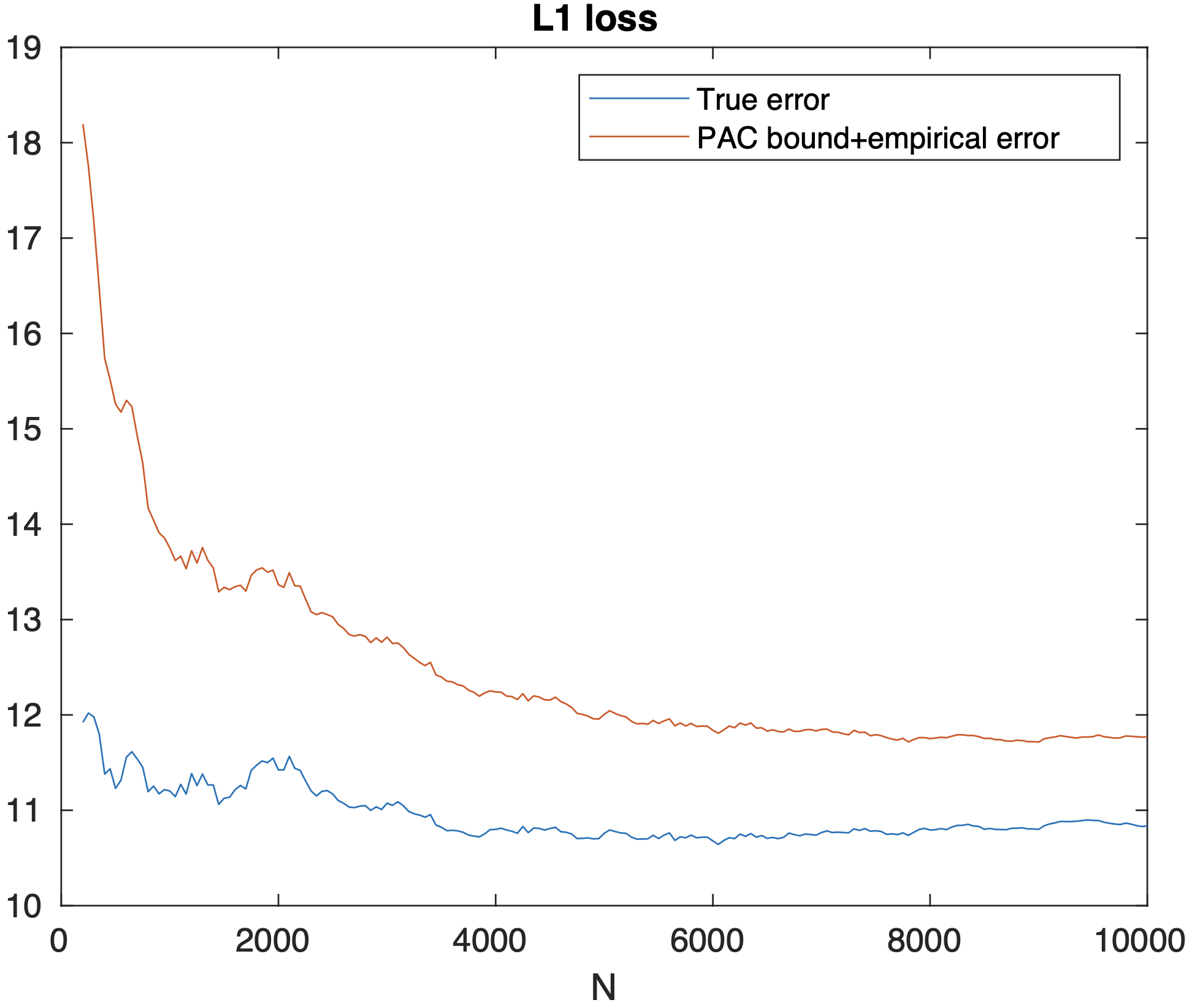
Numerical verification reveals that for each $N$, $\theta$ belongs to $\Theta$. We chose $\delta=0.05$ and we computed $R(\delta)$. We then computed $\mathcal{L}_{N}^{\mathbf{S}}(\Sigma(\theta))$, $\mathcal{L}(\Sigma(\theta))$, using the norm as loss $\ell(y,y^{\prime})=\|y-y^{\prime}\|_{2}$, and by approximating $\mathcal{L}(\Sigma(\theta))$ by the empirical prediction error $\mathcal{L}_{M}^{\mathbf{S}_{val}}(\Sigma(\theta))$ on the validation data set. As Figure 1 shows, $\mathcal{L}(\Sigma(\theta))\leq\mathcal{L}^{S}(\Sigma(\theta))+\frac{R(\delta)}{\sqrt{N}}$ holds, and the resulting bound on the true loss $\mathcal{L}(\Sigma(\theta))$ is not vacuous: the bound for $N=10000$ is smaller than the true loss $\mathcal{L}(\Sigma(\theta))$ for $N=200$.

Refer to caption
Figure 1: Difference between the estimated and the true error. The estimated error is the sum of the empirical error measured on a finite set with $N$ elements and the PAC bound.

VIII Conclusion

In this paper we examined LPV systems within the confines of statistical learning theory and derived a PAC bound on the generalization error under stability conditions. The central element of the proof is the application of Volterra series expansion in order to upper bound the Rademacher complexity of LPV systems. Further research is directed towards extending these methods to more general models, possibly exploiting the powerful approximation properties of LPV systems.

References

  • [1] R. Tóth, Modeling and identification of linear parameter-varying systems, vol. 403. Springer, 2010.
  • [2] B. Bamieh and L. Giarré, “Identification of linear parameter varying models,” Int. Journal of Robust and Nonlinear Control, vol. 12, pp. 841–853, 2002.
  • [3] V. Verdult and M. Verhaegen, “Subspace identification of multivariable linear parameter-varying systems,” Automatica, vol. 38, no. 5, pp. 805–814, 2002.
  • [4] D. Piga, P. Cox, R. Tóth, and V. Laurain, “LPV system identification under noise corrupted scheduling and output signal observations,” Automatica, vol. 53, pp. 329–338, 2015.
  • [5] P. Lopes dos Santos, T. Azevedo Perdicolis, C. Novara, J. Ramos, and D. Rivera, Linear Parameter-Varying System Identification: new developments and trends. Advanced Series in Electrical and Computer Engineering, World Scientific, 2011.
  • [6] T. Oomen and O. Bosgra, “System identification for achieving robust performance,” Automatica, vol. 48, no. 9, pp. 1975–1987, 2012.
  • [7] P. L. dos Santos, J. A. Ramos, and J. L. M. de Carvalho, “Identification of LPV systems using successive approximations,” in Proc. of 47th IEEE Conference on Decision and Control, pp. 4509–4515, 2008.
  • [8] P. Cox, M. Petreczky, and R. Tóth, “Towards efficient maximum likelihood estimation of LPV-SS models,” Automatica, vol. 97, no. 9, pp. 392–403, 2018.
  • [9] L. Ljung, “System identification,” in Signal analysis and prediction, pp. 163–173, Springer, 1998.
  • [10] P. Alquier, “User-friendly introduction to pac-bayes bounds,” arXiv preprint arXiv:2110.11216, 2021.
  • [11] S. Shalev-Shwartz and S. Ben-David, Understanding machine learning: From theory to algorithms. Cambridge university press, 2014.
  • [12] A. Orvieto, S. L. Smith, A. Gu, A. Fernando, C. Gulcehre, R. Pascanu, and S. De, “Resurrecting recurrent neural networks for long sequences,” arXiv preprint arXiv:2303.06349, 2023.
  • [13] P. Kidger, “On neural differential equations,” arXiv preprint arXiv:2202.02435, 2022.
  • [14] A. Gu and T. Dao, “Mamba: Linear-time sequence modeling with selective state spaces,” arXiv preprint arXiv:2312.00752, 2023.
  • [15] A. Isidori, Nonlinear control systems: an introduction. Springer, 1985.
  • [16] A. Krener, “Bilinear and nonlinear realization of input-output maps,” SIAM Journal on Control, vol. 13, no. 4, 1974.
  • [17] M. Vidyasagar and R. L. Karandikar, “A learning theory approach to system identification and stochastic adaptive control,” Probabilistic and randomized methods for design under uncertainty, pp. 265–302, 2006.
  • [18] M. C. Campi and E. Weyer, “Finite sample properties of system identification methods,” IEEE Transactions on Automatic Control, vol. 47, no. 8, pp. 1329–1334, 2002.
  • [19] J. Hanson, M. Raginsky, and E. Sontag, “Learning recurrent neural net models of nonlinear systems,” in Learning for Dynamics and Control, pp. 425–435, PMLR, 2021.
  • [20] P. Koiran and E. D. Sontag, “Vapnik-chervonenkis dimension of recurrent neural networks,” Discrete Applied Mathematics, vol. 86, no. 1, p. 63–79, 1998.
  • [21] P. Kuusela, D. Ocone, and E. D. Sontag, “Learning complexity dimensions for a continuous-time control system,” SIAM journal on control and optimization, vol. 43, no. 3, pp. 872–898, 2004.
  • [22] A. Fermanian, P. Marion, J.-P. Vert, and G. Biau, “Framing rnn as a kernel method: A neural ode approach,” Advances in Neural Information Processing Systems, vol. 34, pp. 3121–3134, 2021.
  • [23] P. Marion, “Generalization bounds for neural ordinary differential equations and deep residual networks,” arXiv preprint arXiv:2305.06648, 2023.
  • [24] J. Hanson and M. Raginsky, “Rademacher complexity of neural odes via chen-fliess series,” arXiv preprint arXiv:2401.16655, 2024.
  • [25] M. Simchowitz, R. Boczar, and B. Recht, “Learning linear dynamical systems with semi-parametric least squares,” in Conference on Learning Theory, pp. 2714–2802, PMLR, 2019.
  • [26] S. Oymak and N. Ozay, “Revisiting ho–kalman-based system identification: Robustness and finite-sample analysis,” IEEE Transactions on Automatic Control, vol. 67, p. 1914–1928, 4 2022.
  • [27] A. Tsiamis, I. Ziemann, N. Matni, and G. J. Pappas, “Statistical learning theory for control: A finite-sample perspective,” IEEE Control Systems Magazine, vol. 43, no. 6, pp. 67–97, 2023.
  • [28] P. Bilingsley, Probability and measure. Wiley, 1986.
  • [29] D. Rácz, M. Gonzalez, M. Petreczky, A. Benczúr, and B. Daróczy, “A finite-sample generalization bound for stable lpv systems,” arXiv preprint arXiv:2405.10054, 2024.
  • [30] L. Zhang and J. Lam, “On $\mathcal{H}_{2}$ model reduction of bilinear systems,” Automatica, vol. 38, pp. 205–216, 2002.
  • [31] M. Sznaier, T. Amishima, P. Parrilo, and J. Tierno, “A convex approach to robust h2 performance analysis,” Automatica, vol. 38, no. 6, pp. 957–966, 2002.
  • [32] P. den Boef, P. B. Cox, and R. Tóth, “Lpvcore: Matlab toolbox for lpv modelling, identification and control,” IFAC-PapersOnLine, vol. 54, no. 7, pp. 385–390, 2021. 19th IFAC Symposium on System Identification SYSID 2021.

IX Appendix A: Proof of Lemma IV.1

Consider the following bilinear system for all $i_{q},i_{r}\in[n_{\text{p}}]$ for a fixed $t\in[0,T]$.

$$\begin{split}&\dot{s}(\tau)=\Bigg{(}A_{0}+\frac{\lambda}{2}I+\sum\limits_{i=1}^{n_{\text{p}}}p_{i}(\tau+T-t)A_{i}\Bigg{)}s(\tau),\\ &y^{s,t}(\tau)=C_{i_{q}}s(\tau),~{}s(0)=B_{i_{r}}u(T-t)e^{-\frac{\lambda}{2}t}.\end{split}$$ (3)

From the Volterra series representation [15] of bilinear systems we have

$\displaystyle y^{s,t}_{i_{q},i_{r}}(\tau)$ $\displaystyle=\Big{[}w_{i_{q},i_{r},\emptyset}(\tau)+$
$\displaystyle\sum\limits_{k=1}^{\infty}\sum\limits_{\mathbf{I}\in I_{k}}\int_{\Delta_{k}^{\tau}}w_{i_{q},i_{r},\mathbf{I}}^{\lambda,\tau}(\boldsymbol{\tau})p_{\mathbf{I}}(\boldsymbol{\tau})d\boldsymbol{\tau}\Big{]}u(T-t)e^{-\frac{\lambda}{2}t}$

where $p_{I}$ is as in Section IV and $w_{i_{q},i_{r},I}^{\lambda,\tau}(\boldsymbol{\tau})=w_{i_{q},i_{r},I}^{\lambda}((\tau,\boldsymbol{\tau}))$, for all $I\in I_{k}$ and $\boldsymbol{\tau}\in\Delta_{k}^{\tau}$, $k>0$. By [1, Chapter 3.3.1.1]

$$y_{\Sigma}(u,p)(T)\!\!=\!\!\int_{0}^{T}\!\!C(p(T))\Phi(T,T-t)B(p(T-t))u(T-t)dt$$

where $\Phi(s,s_{0})$ is the fundamental matrix of $\dot{z}(s)=A(p(s))z(s)$. Since the fundamental matrix $\Phi_{\lambda}(s,s_{0})$ of $\dot{z}(s)=(A(p(s))+\frac{\lambda}{2}I)z(s)$ satisfies $\Phi_{\lambda}(s,s_{0})=e^{\frac{\lambda}{2}(s-s_{0})}\Phi(s,s_{0})$, we have $s(\tau)=\Phi_{\lambda}(T-t+\tau,T-t)B_{i_{r}}u(T-t)e^{-\frac{\lambda}{2}t}=e^{\frac{\lambda}{2}(t-\tau)}\Phi(T-t+\tau,T-t)B_{i_{r}}u(T-t)$. Then from the definition of $C(p(T))$ and $B(p(T-t))$,

$$y_{\Sigma}(u,p)(T)=\int_{0}^{T}\sum\limits_{i_{q},i_{r}=0}^{n_{\text{p}}}p_{i_{q}}(T)p_{i_{r}}(T-t)y_{i_{q},i_{r}}^{s,t}(t)\,dt.$$

Applying the Volterra expansion above together with
$\{(t,\boldsymbol{\tau})\mid t\in[0,T],\boldsymbol{\tau}\in\Delta_{k}^{t}\}=\Delta^{T}_{k+1}$ yields the result.  ∎

X Appendix B: proof of Lemma IV.4 and bounding the $H_{2}$ norms

If Assumption IV.3 holds, then $A_{0}^{T}Q+QA_{0}\prec-\lambda Q$, and hence $A_{0}+\lambda I$ is Hurwitz. Let $S=A_{0}^{T}Q+QA_{0}+\sum\limits_{i=1}^{n_{\text{p}}}A_{i}^{T}QA_{i}+\sum\limits_{i=1}^{n_{\text{p}}}C_{i}^{T}C_{i}+C_{0}^{T}C_{0}+\lambda Q$. Then $S\prec 0$ and hence $S=-VV^{T}$ for some $V$. Define $\tilde{C}=\begin{bmatrix}C_{0}^{T}&\ldots&C_{n_{\text{p}}}^{T}&V^{T}\end{bmatrix}^{T}$, $\tilde{A}=(A+0.5\lambda I)$ and $N_{i}=A_{i}$, $i\in[n_{\text{p}}]$. Then $\tilde{A}^{T}Q+Q\tilde{A}+\sum_{i=1}^{n_{\text{p}}}N_{i}^{T}QN_{i}+\tilde{C}^{T}\tilde{C}=0$ and hence, by [30, Theorem 6], for any choice of the matrix $G=\begin{bmatrix}G_{1}&\ldots&G_{n_{\text{p}}}\end{bmatrix}$, the bilinear system

$$S(G)\left\{\begin{array}[]{rl}\dot{z}(t)&=\tilde{A}z(t)+\sum_{i=1}^{n_{\text{p}}}\left(N_{i}z(t)p_{i}(t)+G_{i}p_{i}(t)\right)\\ \tilde{y}(t)&=\tilde{C}z(t),~{}z(0)=0,\end{array}\right.$$

has a finite $H_{2}$ norm $\left\lVert S(G)\right\rVert_{H_{2}}$ which satisfies $\left\lVert S(G)\right\rVert_{H_{2}}^{2}=\mathrm{trace}(G^{T}QG)$, and which is defined via Volterra kernels as follows. For each $i\in[n_{\text{p}}]$, let $g_{i,\emptyset}^{G}(t)=\tilde{C}e^{\tilde{A}t}G_{i}$ and for every $I\in I_{k}$, $k>0$, let $g_{i,I}^{G}(t)=\tilde{C}e^{\tilde{A}t_{k+1}}N_{i_{k}}e^{\tilde{A}t_{k}}\cdots e^{\tilde{A}t_{2}}N_{i_{1}}e^{\tilde{A}t_{1}}G_{i}$, $t=(t_{k+1},\ldots,t_{1})\in\mathbb{R}^{k}$, $t\in\mathbb{R}$. Then

$\displaystyle\left\lVert S(G)\right\rVert_{H_{2}}^{2}$ $\displaystyle=\sum_{i=1}^{n_{\text{p}}}\sum_{k=0}^{\infty}\sum_{I\in I_{k}}\int\limits_{[0,+\infty)^{k+1}}\left\lVert g_{i,I}^{G}(t)\right\rVert_{2}^{2}dt.$

Let $G^{i,j}$ be the matrix of which the first column is the $j$th column of $B_{i}$ and all the other elements are zero, $i\in[n_{\text{p}}]$, $j\in[n_{\text{in}}]$. By choosing $G=G^{i,j}$, it follows that the $j$th row of $w_{i_{q},i_{r},I}^{\lambda}(\tau)$ is the $(i_{q}+1)$-th row of $g^{G^{i,j}}_{i_{r},I}(t)$ where $\tau\in\Delta_{k+1}^{\infty}$ and $t=(\tau_{k+1}-\tau_{k},\ldots,\tau_{2}-\tau_{1},\tau_{1})$, $i_{q},i_{r}\in[n_{\text{p}}]_{0}$, $I\in I_{k}$, $k\geq 0$. Hence, $\sum_{j=1}^{n_{\text{in}}}\left\lVert g_{i_{r},I}^{G^{i_{r},j}}(\tau)\right\rVert_{2}^{2}\geq\sum_{i_{q}=0}^{n_{\text{p}}}\left\lVert w_{i_{q},i_{r},I}^{\lambda}(\tau)\right\rVert_{2}^{2}$, and by applying a change of variables in the iterated integrals,

$\displaystyle\sum_{i_{q},i_{r}=0}^{n_{\text{p}}}\sum_{k=0}^{\infty}\sum_{I\in I_{k}}\int_{\Delta_{k+1}^{t}}\left\lVert w^{\lambda}_{i_{q},i_{r},I}(\tau)\right\rVert^{2}_{2}d\tau\leq$
$\displaystyle\sum_{i_{r}=0}^{n_{\text{p}}}\sum_{j=1}^{n_{\text{in}}}\left\lVert S(G^{i_{r},j})\right\rVert_{H_{2}}^{2}=\sum_{i_{r}=0}^{n_{\text{p}}}\mathrm{trace}(B_{i_{r}}^{T}QB_{i_{r}}).$

In the last step we used the fact that $\sum_{j=1}^{n_{\text{in}}}\mathrm{trace}((G^{i_{r},j})^{T}QG^{i_{r},j})=\mathrm{trace}(B_{i_{r}}^{T}QB_{i_{r}})$

Finally, from Lemma VI.2 it follows that $y_{\Sigma}(u,p)(T)=\langle w^{T,\Sigma},\varphi^{T,u,p}\rangle_{\mathcal{H}}$ for a suitable Hilbert space. From the definition of $w^{T,\Sigma}$ and $\varphi^{T,u,p}$ and the proof of Lemma VI.2 it follows that $\|w^{T,\Sigma}\|_{\mathcal{H}}\leq\|\Sigma\|_{\lambda,H_{2}}$, $\|\varphi^{T,u,p}\|_{\mathcal{H}}\leq(n_{\text{p}}+1)\|u\|_{L^{2}([0,T],\mathbb{R}^{n_{\text{in}}})}$ and hence by the Cauchy-Schwartz inequality the result follows.  ∎

Bounding the $H_{2}$ norms. Below we present a sufficient condition for computing an upper bound on the $H_{2}$ norms of models from $\mathcal{E}$.

Assumption X.1

There exists a positive real number $\gamma>0$ and $\Gamma>0$ such that $\gamma\geq\Gamma+n_{\text{p}}$ and for every $\Sigma\in\mathcal{E}$ of the form (1), $\Gamma\geq\sup_{i=1}^{n_{\text{p}}}\left\lVert A_{i}\right\rVert^{2}_{2}n_{\text{p}}$ and $\left\lVert e^{A_{0}t}\right\rVert_{2}\leq e^{-\frac{\gamma}{2}t}$.

Lemma X.2

If Assumption X.1 holds then (2) holds with any $n_{\text{p}}\leq\lambda\leq\gamma-\Gamma$ and $Q=I$, and

$\displaystyle c_{\mathcal{E}}\leq(n_{\text{p}}+1)^{2}K^{2}_{C}K^{2}_{B}\Big{(}\frac{1}{\lambda}+\frac{1}{\gamma-\lambda+\Gamma}\Big{)}$

where $K_{B}=\sup_{i=1}^{n_{\text{p}}}\left\lVert B_{i}\right\rVert_{2}$, $K_{C}=\sup_{i=1}^{n_{\text{p}}}\left\lVert C_{i}\right\rVert_{2}$.

The proof follows from a simple calculation followed by applying Lemma IV.4.

XI Appendix C: multi output

Let use assume that the loss functions satisfies the following condition: $\ell(y,\tilde{y})=\sum_{j=1}^{p}\ell_{i}(y^{j},\tilde{y}^{j})$, where $y^{j},\tilde{y}^{j}$ denote the $j$th component of the vectors $y^{j},\tilde{y}^{j}\in\mathbb{R}^{p}$ respectively and $\ell_{j}$ are Lipschitz functions with Lipschitz constant $K_{\ell}$. For instance, if $\ell(y,\tilde{y})=\|y-y^{{}^{\prime}}\|_{1}$ is the $\ell_{1}$ loss, or $\ell(y,y^{{}^{\prime}})=\|y-y^{{}^{\prime}}\|_{2}^{2}$ is the classical quadratic loss and $y,y^{{}^{\prime}}$ are bounded, then this assumption is satisfied. For all $\Sigma\in\mathcal{E}$, let $\Sigma_{j}$ be the LPV system which arises from $\Sigma$ by considering only the $j$th output, and let $\mathcal{E}_{j}$ be the class of LPV systems formed by all $\Sigma_{j}$, $\Sigma\in\mathcal{E}_{j}$. For every $j=1,\ldots,n_{\text{out}}$, consider the data set $\mathbf{S}_{j}=\{(u_{i},p_{i},y_{i}^{j})\}_{1\leq i\leq N}$, which is obtained from the data set $\mathbf{S}$ by taking only the $j$th component of the true outputs $\{y_{i}\}_{i=1}^{n}$. Then it follows that $\mathcal{L}(\Sigma)=\sum_{j=1}^{n_{\text{out}}}\mathcal{L}(\Sigma_{j})$, where $\mathcal{L}(\Sigma_{j})=\mathbb{E}_{(u,p,y)\sim\mathcal{D}}[\ell_{j}(y_{\Sigma_{j}}(u,p)(T),y^{j}(T))]$ and $\mathcal{L}_{N}^{\mathbf{S}}(\Sigma)=\sum_{j=1}^{n_{\text{out}}}\mathcal{L}_{N}^{\mathbf{S}_{j}}(\Sigma_{j})$. By applying the main theorem of the paper to $\mathbf{S}_{j}$ and $\mathcal{E}_{j}$, $j=1,\ldots,n_{\text{out}}$, it follows that

$\displaystyle\mathbb{P}_{\mathbf{S}\sim\mathcal{D}^{N}}\Bigg{(}\forall\Sigma_{j}\in\mathcal{E}_{j}:\mathcal{L}(\Sigma_{j})-\mathcal{L}^{\mathbf{S}_{j}}_{N}(\Sigma_{j})\leq\frac{R_{j}\delta)}{\sqrt{N}}\Bigg{)}\geq 1-\delta.$

for all $j=1,\ldots,n_{\text{out}}$. Then by using the union bound it follows that

$\displaystyle\mathbb{P}_{\mathbf{S}\sim\mathcal{D}^{N}}\Bigg{(}\forall j=1,\ldots,n_{\text{out}},~{}\forall\Sigma_{j}\in\mathcal{E}_{j}:\mathcal{L}(\Sigma_{j})-\mathcal{L}^{\mathbf{S}_{j}}_{N}(\Sigma_{j})$
$\displaystyle\leq\frac{\max_{1\leq j\leq n_{\text{out}}}R_{j}(\delta)}{\sqrt{N}}\Bigg{)}\geq 1-n_{\text{out}}\delta.$

and by using $\mathcal{L}(\Sigma)=\sum_{j=1}^{n_{\text{out}}}\mathcal{L}(\Sigma_{j})$ and $\mathcal{L}_{N}^{\mathbf{S}}(\Sigma)=\sum_{j=1}^{n_{\text{out}}}\mathcal{L}_{N}^{\mathbf{S}_{j}}(\Sigma_{j})$ it then follows that

$\displaystyle\mathbb{P}_{\mathbf{S}\sim\mathcal{D}^{N}}\Bigg{(}\forall\Sigma\in\mathcal{E}:\mathcal{L}(\Sigma)-\mathcal{L}^{\mathbf{S}}_{N}(\Sigma)$
$\displaystyle\leq\frac{\max_{1\leq j\leq n_{\text{out}}}R_{j}(\delta)}{\sqrt{N}}\Bigg{)}\geq 1-n_{\text{out}}\delta.$

XII Appendix D: Computing $\theta$ in numerical example

We compute the estimate $\hat{\theta}$ of $\theta$ so that $a(\hat{\theta})$, is the least squares solution of $y_{i,k}=\begin{bmatrix}y_{i,k-1}&y_{i,k-2}&y_{i,k-2}p_{i,k-2}&u_{i,k-2}\end{bmatrix}a(\theta)$, $i=1,\ldots,N$, $k=45$, where where the function function $a(\theta)$ is

$$a(\theta)=\begin{bmatrix}2(1-\frac{T_{s}}{\theta_{1}}),&(1-\frac{T_{s}}{\theta_{1}})^{2},&T_{s}^{2}\theta_{2},&\theta_{3}T_{s}^{2}\end{bmatrix}^{T},$$

$y_{i,l}=y_{i}(lT_{s})$, $u_{i,l}=u_{i}(lT_{s})$, and $p_{i,l}=p_{i}(lT_{s})$ for all $l\in\mathbb{N}$.

XIII Appendix E: difference between minimal prediction error models and best possible models

Consider the minimal prediction error model $\hat{\Sigma}=\mathrm{argmin}_{\Sigma\in\mathcal{E}}\mathcal{L}^{S}_{N}(\Sigma)$ and the best possible model: $\Sigma_{\star}=\mathrm{argmin}_{\Sigma\in\mathcal{E}}\mathcal{L}(\Sigma)$, see [29].

Corollary XIII.1

With the notation of Theorem V.1 and with $R(\delta):=c\left(2+5\sqrt{2\log(8/\delta)}\right)$ , for any $\delta\in[0,\delta]$

$\displaystyle\mathbb{P}_{\mathbf{S}\sim\mathcal{D}^{N}}\Bigg{(}\mathcal{L}(\hat{\Sigma})\leq\mathcal{L}(\Sigma_{\star})+\frac{R_{2}(\delta)}{\sqrt{N}}\Bigg{)}\geq 1-\delta.$

That is, we can determine the minimal number of data points $N_{min}=(\frac{R_{2}(\delta)}{\epsilon})^{2}$, such that the difference between the performance of the minimal prediction error model and that of the best possible model is below the desired threshold $\epsilon$.