High-Scale SUSY from Sgoldstino Inflation

Abstract:

We review a number of unimodular no-scale supergravity models with F-term SUSY breaking which support technically natural de Sitter vacua. A variant of these models develops a stage of inflection-point inflation which can be realized for subplanckian field values consistently with the observational data. For central value of the spectral index $n_{\rm s}$, the necessary tuning is of the order of $10^{-6}$, the tensor-to-scalar ratio is tiny whereas the running of $n_{\rm s}$ is around $-3\cdot 10^{-3}$. Our proposal is compatible with high-scale SUSY and the results of LHC on the Higgs boson mass.

1 Outline

In this talk we first – see Sec. 2 – review a set of (generalized) no-scale models (nSMs) [1, 2] within Supergravity (SUGRA) which assure spontaneous Supersymmetry (SUSY) breaking at a technically natural de Sitter (dS) vacuum. As a result, the problem of Dark Energy (DE) can be explained by fine tuning just one superpotential coupling. We then, in Sec. 3, concentrate on a specific model which offers a coexistence of the aforementioned dS vacuum with an inflection point of the potential developed at larger field values and, in Sec. 4, we investigate the communication of SUSY breaking in the observable sector of minimal SUSY standard model (MSSM). Finally, in Sec. 5 we show how we can obtain Inflection-Point Inflation (IPI) [3] in our set-up and in Sec. 6 we delineate regions of parameters allowed by the observations [5, 4, 6]. Sec. 7 summarizes our conclusions and discusses some open issues.

Unless otherwise stated, we use units where the reduced Planck scale $m_{\rm P}=2.4\cdot 10^{18}~{}{\mbox{\rm GeV}}$ is taken to be unity, a subscript of type $,\chi$ denotes derivation with respect to (w.r.t.) the field $\chi$ and charge conjugation is denoted by a star.

2 From Minkowski to dS Vacua In No-Scale SUGRA

We here provide a short introduction on SUSY breaking within SUGRA in Sec. 2.1 and then, we show how this mechanism is systematized within no-scale SUGRA obtaining Minkowski (see Sec. 2.2) or dS vacua – see Sec. 2.3. Examples of such nSMs are given in Sec. 2.4.

2.1 SUSY breaking within SUGRA

Within global SUSY, the scalar potential of a gauge-singlet superfield $Z$, $V_{\rm SUSY}$, is positive semi-definite, since

$$V_{\rm SUSY}=|F_{Z}|^{2}~{}~{}\mbox{with}~{}~{}F_{Z}=\partial_{Z}W.$$ (1)

Here $W=W(Z)$ is an holomorphic function named superpotential. Spontaneous SUSY breaking occurs when $\langle{F_{Z}}\rangle\neq 0$ which results to $\langle{V_{\rm SUSY}}\rangle^{1/4}>0$. The non discovery of SUSY in LHC dictates $\langle{F_{Z}}\rangle^{1/2}>1~{}{\mbox{\rm TeV}}$. On the other hand, $\langle{F_{Z}}\rangle^{1/2}$ may be identified with the cosmological constant $\Lambda_{\rm CC}\simeq 2.3~{}{\rm meV}$. Therefore, we obtain an inconsistency. The spontaneous SUSY breaking is accompanied with the presence of a massless fermion named goldstino and for this reason its SUSY partner, $Z$, is called sgoldstino.

Within local SUSY – i.e. SUGRA – the F-term scalar potential is given by

$$V_{\rm SUGRA}=e^{G}\left(G^{ZZ^{*}}G_{Z}G_{Z^{*}}-3\right)~{}~{}\mbox{where}~{}~{}G:=K+\ln|W|^{2}$$ (2)

is the Kähler-invariant function and $K=K(Z,Z^{*})$ the Kähler potential. Also $G_{ZZ^{*}}=K_{ZZ^{*}}=\partial_{Z}\partial_{Z^{*}}K$ is the Kähler metric and $K^{ZZ^{*}}=K_{ZZ^{*}}^{-1}$. In this context, SUSY is broken again when $\langle{F^{Z}}\rangle\neq 0$ where $F^{Z}=e^{G/2}K^{ZZ^{*}}G_{Z^{*}}$ which may occur with $\langle{V_{\rm SUGRA}}\rangle\simeq 0$. This mechanism is accompanied with the absorption of the goldstino by the gravitino, $\widetilde{G}$, which acquires mass according to “super-Higgs” mechanism

$$m_{3/2}=\langle{e^{G/2}}\rangle=\langle{e^{K/2}W}\rangle=\langle{G_{Z{Z^{*}}}F^{Z}\bar{F}^{Z^{*}}-V_{\rm SUGRA}}\rangle^{1/2}/\sqrt{3}.$$ (3)

Based on this formalism we can obtain several models of SUSY breaking [7, 9, 10, 8]. One of the key ingredients for the successful implementation of this scenario is the determination of a naturally realistic vacuum for $V_{\rm SUGRA}$ which may be Minkowski for $\langle{V_{\rm SUGRA}}\rangle=0$ or de Sitter for $\langle{V_{\rm SUGRA}}\rangle>0$.

2.2 Minkowski Vacua In no-scale SUGRA

Within no-scale SUGRA [1], SUSY is broken along an F-flat direction which naturally yields $V_{\rm SUGRA}=0$. To construct systematically nSMs, we use as input $K$ and determine $W$ so as $V_{\rm SUGRA}=0$. I.e., we solve the differential equation

$$0=e^{K}\left(g_{K}^{-1}\left|\partial_{Z}W+WK_{Z}\right|^{2}-3|W|^{2}\right),~{}~{}\mbox{where}~{}~{}g_{K}^{-1}=K_{ZZ^{*}}^{-1}=K^{ZZ^{*}}$$ (4)

assuming that the direction $Z=Z^{*}$ is stable – this assumption can be verified a posteriori. Indeed, solving Eq. (4) w.r.t $W=W_{0}(Z)$ we find

$$\frac{dW_{0}}{dZW_{0}}=\pm\sqrt{3g_{K}}-K_{Z}~{}~{}\Rightarrow~{}~{}W_{0}^{\pm}=m\exp\left(\pm\int dZ\sqrt{3g_{K}}-\int dZK_{Z}\right).$$ (5)

with ${}^{\prime}=d/dZ$. E.g., if we select the Kähler potential:

• $K=-3\ln(T+T^{*})$ we obtain the well-known results [11] $W_{0}^{-}=m$ but also $W_{0}^{+}=8mT^{3}$ ;

• $K=|Z|^{2}$ we obtain $W_{0}^{\pm}=me^{\pm\sqrt{3}Z-Z^{2}/2}$. Therefore we can obtain a nSM even with flat geometry. This is a totally novel result [2].

2.3 dS Vacua In no-Scale SUGRA

The models can be extended to support dS vacua. In this case $\langle{V_{\rm SUGRA}}\rangle$ may account for DE without requiring any external mechanism for vacuum uplifting [9]. To accomplish this extra achievement we consider the following linear combination of $W_{0}^{\pm}$

$$W_{\Lambda}=W_{0}^{+}-C_{\Lambda}W_{0}^{-}$$ (6)

and we obtain the SUGRA potential

$$V_{\Lambda}=e^{K}\left(g_{K}^{-1}\left(W_{\Lambda}^{\prime}+W_{\Lambda}K_{Z}\right)^{2}-3W_{\Lambda}^{2}\right)=12e^{K}C_{\Lambda}W_{0}^{-}W_{0}^{+}=12m^{2}C_{\Lambda}.$$ (7)

Finely tuning $C_{\Lambda}$ to a value $C_{\Lambda}\simeq 10^{-108}$ for $m\sim 10^{-6}$, e.g, we may identify $V_{\Lambda}$ with the present DE energy density, i.e.,

$$V_{\Lambda}=\Omega_{\Lambda}\rho_{\rm c}=7.3\cdot 10^{-121}m_{\rm P}^{4},$$ (8)

where the density parameter of DE $\Omega_{\Lambda}$ and the current critical energy density of the universe $\rho_{\rm c}$ are given in Ref. [4].

2.4 Realistic nSMs

Although quite appealing, the nSMs above develop a completely flat $V_{\rm SUGRA}$, I.e.

$$V_{\rm SUGRA}=V^{\prime}_{\rm SUGRA}=V^{\prime\prime}_{\rm SUGRA}=0.$$ (9)

Therefore $m_{3/2}$ and the soft SUSY-breaking terms remain undetermined. Moreover, a massless mode arises in the spectrum. To cure these drawbacks, we may include in $K$ a stabilization (higher order) term

$$-k^{2}Z_{\rm v}^{4}~{}~{}\mbox{with}~{}~{}Z_{\rm v}=Z+Z^{*}-\sqrt{2}{\rm v}$$ (10)

which selects the vacuum $(\langle{z}\rangle,\langle{{\bar{z}}}\rangle)=({\rm v},0)$ from the flat direction and provides the real component of sgoldstino with mass. The presence of $k$-dependent term is natural according to ’t Hooft argument [12] since for $k\rightarrow 0$ the symmetry becomes exact. The selection of this higher order term is arbitrary, though.

nSM	$K$	$W_{0}^{\pm}/m$	$W_{\Lambda}/m$	Enhanced Symmetry
				of the Kähler  Manifold
1	$-N\ln\left(T+T^{*}+k^{2}T_{\rm v}^{4}/N\right),$	$(2T)^{n_{\mp}},$ where	$(2T)^{n_{+}}C_{T}^{-},$ where	$SU(1,1)/U(1)$
	$T_{\rm v}=T+T^{*}-\sqrt{2}{\rm v},N>0$	$n_{\pm}=(N\pm\sqrt{3N})/2$	$C_{T}^{-}=1-C_{\Lambda}(2T)^{-\sqrt{3N}}$	i.e., Hyperbolic Geometry with
2	${\boldmath-}N\ln\left(1{\boldmath-}|Z|^{2}/N+k^{2}Z_{\rm v}^{4}/N\right),$	$v_{\bm{-}}^{-N/2}u_{\bm{-}}^{\pm 1},$ where	$v_{\bm{-}}u_{\bm{-}}C_{u\bm{-}}^{-},$ where	$\bullet$ Half-plane coordinates for nSM1
	$Z_{\rm v}=Z+Z^{*}-\sqrt{2}{\rm v},N>0$	$v_{\bm{-}}=1{\boldmath-}Z^{2}/N$	$C_{u\bm{-}}^{-}=1-C_{\Lambda}u_{\bm{-}}^{-2}$	$\bullet$ Poincaré-disc coordinates for nSM2
		$u_{\bm{-}}=e^{\sqrt{3N}{\boldmath{\rm atnh}}(Z/N)}$	${\rm atnh}:={\rm arctanh}$
3	${\boldmath+}N\ln\left(1{\boldmath+}|Z|^{2}/N-k^{2}Z_{\rm v}^{4}/N\right),$	$v_{\bm{+}}^{-N/2}u_{\bm{+}}^{\pm 1},$ where	$v_{\bm{+}}u_{\bm{+}}C_{u\bm{+}}^{-},$ where	$SU(2)/U(1)$
	$Z_{\rm v}=Z+Z^{*}-\sqrt{2}{\rm v},N>0$	$v_{\bm{+}}=1{\boldmath+}Z^{2}/N$	$C_{u\bm{+}}^{-}=1-C_{\Lambda}u_{\bm{+}}^{-2}$	i.e., Compact Geometry
		$u_{\bm{+}}=e^{\sqrt{3N}{\boldmath{\rm atn}}(Z/N)}$	${\rm atn}=\arctan$
4	$|Z|^{2}-k^{2}Z_{\rm v}^{4},$	$wf^{\pm 1},$ where	$wfC_{f}^{-},$ where	$U(1)$
	$Z_{\rm v}=Z+Z^{*}-\sqrt{2}{\rm v}$	$w=e^{-Z^{2}/2}$ and $f=e^{\sqrt{3}Z}$	$C_{f}^{-}=1-C_{\Lambda}f^{-2}$	i.e., Flat Geometry

Table 1: Uni-Modular no-Scale Models (nSMs) with dS vacua.

Applying the procedure above several nSMs with dS vacua can be established varying the Kähler  geometry. In Table 1 we arrange a catalogue of such models based exclusively on one modulus. These models are introduced in Ref. [2] where multi-moduli models are also exposed – see also Ref. [1]. For each nSM we can see there the adopted Kähler potential, the solutions of Eq. (5) and the resulting $W_{\Lambda}$ from Eq. (6). The enhanced symmetry (for $k\rightarrow 0$) of the Kähler manifold is also shown in the rightmost column of Table 1. For $k=0$ the Kähler manifold of nSM1 enjoys the $SU(1,1)/U(1)$ hyperbolic symmetry parameterized by the half-plane coordinates $T$ and $T^{*}$. As a result, the expression in Eq. (5) is a polynomial of $2T$. For the well-known nSM with $N=3$ [11], we obtain $n_{+}=3$ and $n_{\bm{-}}=0$ and so, we have the ingredients

$$K=-3\ln(T+T^{*})\>\>\mbox{and}\>\>W_{\Lambda}=8mT^{3}C_{T}^{-}\>\>\mbox{where}\>\>C_{T}^{-}=1-C_{\Lambda}(2T)^{-3}.$$ (11)

The same enhanced symmetry parameterized in the Poincaré-disc coordinates $Z$ and $Z^{*}$ is valid for nSM2. That parametrization allows us to pass from the non-compact to the compact geometry of nSM3 by changing the signs in the relevant $K$’s. As a consequence we obtain a remarkable correspondence between nSM2 and nSM3 as regards the relevant expressions of $W_{0}^{\pm}$. Namely $v_{\bm{-}}$ and ${\rm arctanh}$ in nSM2 are replaced by $v_{\bm{+}}$ and $\arctan$ in nSM3. Finally, we consider nSM4 where a flat Kähler potential is adopted resulting to exponential $W_{0}^{\pm}$.

To check the stability of the vacuum of the nSMs in Table 1, we derive the mass spectrum at the vacuum. The results are presented in Table 2. We remark that we need $k>0$ and $N>3$ when the (enhanced) Kähler  geometry is hyperbolic. In a such case we also obtain real values for the mass $m_{{\bar{z}}}$ of the imaginary component of $Z$. Note that we here decompose $Z$ as $Z=(z+i{\bar{z}})/\sqrt{2}$.

	Mass Of Sgoldstino Components		$m_{3/2}$	Restriction
nSM	Real	Imaginary
1	$24k{\rm v}^{3/2}m_{3/2}$	$2(1-3/N)^{1/2}m_{3/2}$	$m(2{\rm v}^{2})^{\sqrt{3N}/4}$	$N>3$
2	$12k\langle{v_{\bm{-}}}\rangle^{3/2}m_{3/2}$	$2(1-3/N)^{1/2}m_{3/2}$	$m\langle{u_{\bm{-}}}\rangle$	$N>3$
3	$12k\langle{v_{\bm{+}}}\rangle^{3/2}m_{3/2}$	$2(1+3/N)^{1/2}m_{3/2}$	$m\langle{u_{\bm{+}}}\rangle$	-
4	$12km_{3/2}$	$2m_{3/2}$	$me^{\sqrt{3/2}{\rm v}}$	-

Table 2: Particle mass spectrum at the vacuum for the nSMs presented in Table 1.

3 DE and Inflection Point From no-Scale SUGRA

We aspire to identify the radial component of the sgoldstino $Z$ with the inflaton – for similar attempts see Ref. [13]. We accomplish this aim by localizing an inflection point of the potential $V_{\rm SUGRA}(Z)$. Close to it we may obtain a stage of IPI according to formalism discussed in Ref. [14, 15]. To achieve it for $z>{\rm v}$ we adopt nSM1 in Table 1 with $T=1/2-Z/2$. I.e., we set

$$K=-N\ln\Omega\>\>\>\mbox{with}\>\>\>\Omega=1-(Z+Z^{*})/2+k^{2}Z_{\rm v}^{4}\>\>\>\mbox{and}\>\>\>Z_{\rm v}=Z+Z^{*}-2{\rm v}.$$ (12)

For $k=0$, $K$ enjoys a symmetry related to a subset of $U(1,1)$ without to define specific Kähler  manifold [16]. Repeating the procedure in Sec. 2, we find that $K$ may be associated with

$$W_{\Lambda}=m\omega^{n_{+}}C_{\omega}^{-}\>\>\>\mbox{with}\>\>\>n_{+}=(N+\sqrt{3N})/2,$$ (13)

$$\omega=\Omega(Z=Z^{*},k=0)=1-Z\>\>\>\>\mbox{and}\>\>C_{\omega}^{-}=1-C_{\Lambda}\omega^{-\sqrt{3N}}$$ (14)

where $m$ is an arbitrary mass scale which is constrained to values close to $10^{-7}$ from the normalization of $A_{\rm s}$ – see below.

$m/m_{\rm P}$	$C_{\Lambda}/10^{-108}$	$k/0.1$
$5.6\cdot 10^{-7}$	$2.5$	$4.0167291$
${\rm v}/m_{\rm P}$	$N$	$(n_{+},n_{-})$
$0.5$	$12$	$(9,3)$

Figure 1: The (dimensionless) SUGRA potential $10^{2}V_{\Lambda}/m^{2}m_{\rm P}^{2}$ in Eq. (3.5) as a function of $z$ and ${\theta}$ defined above Eq. (3.6). The location of the dS vacuum at $(\langle{z}\rangle,{\theta})=(0.5,0)$ and the inflection point at $(z_{0},{\theta})\simeq(0.71,0)$ is also depicted by two thick points. The input parameters are listed in the Table.

The exponents $n_{+}$ in Eq. (13) may, in principle, acquire any real value, if we consider $W_{\Lambda}$ as an effective superpotential. When $N/3>1$ is a perfect square, integer $n_{\pm}$ values may arise too. E.g.,

For $$N=12,27 48 (n_{-},n_{+})=(3,9),(9,18) (18,30)$$ and we obtain and respectively. (15)

The resulting SUGRA potential is [3]

$$V_{\Lambda}(Z)=m^{2}\Omega^{-N}\omega^{2n_{+}}\left(|U/2\omega|^{2}-3|C_{\omega}^{-}|^{2}\right),$$ (16)

where we define the auxiliary quantity

$$U=\frac{\sqrt{2N}}{J\Omega}\Bigg{(}\left(\sqrt{3}C_{\omega}^{+}+\sqrt{N}C_{\omega}^{-}\right)\Omega+2\sqrt{N}C_{\omega}^{-}\Omega_{,Z}\omega\Bigg{)}.$$ (17)

The canonically normalized components of the complex scalar field $Z=ze^{i\theta}$ are

$$\frac{d\widehat{z}}{dz}=\sqrt{2K_{ZZ^{*}}}=J~{}~{}\mbox{and}~{}~{}\widehat{\theta}=Jz\theta,$$ (18)

where $J$ can be expressed in terms of $\Omega$ as follows

$$J=\sqrt{2N}\left(\frac{\Omega_{,Z}^{2}}{\Omega^{2}}-\frac{\Omega_{,ZZ^{*}}}{\Omega}\right)^{1/2}\>\>\mbox{with}~{}~{}\Omega_{,Z}=-1/2+4k^{2}Z_{\rm v}^{3}~{}~{}\mbox{and}~{}~{}\Omega_{,ZZ^{*}}=12k^{2}Z_{\rm v}^{2}.$$ (19)

If we plot $10^{2}V_{\Lambda}/m^{2}m_{\rm P}^{2}$ as a function of $z$ and $\theta$ for the inputs in shown the Table of Fig. 1 we see that $V_{\Lambda}$ develops two critical points: The SUSY-breaking dS vacuum which is

$$\langle{z}\rangle={\rm v}~{}~{}\mbox{and}~{}~{}\langle{\theta}\rangle=0~{}~{}\mbox{with}~{}~{}\langle{V_{\Lambda}}\rangle=12C_{\Lambda}m^{2}$$ (20)

and an inflection point for $z=z_{0}\simeq 0.71>{\rm v}$ which lets open the possibility of an inflationary stage. The vacuum in Eq. (20) is stable against fluctuations of the various excitations for $N>3$ which assures $m_{\theta}^{2}>0$ in accordance with our findings in Table 2. Indeed, we find

$$m_{z}\simeq 48m_{3/2}kN^{-1/2}\langle{\omega}\rangle^{3/2}\>\>\>\mbox{and}\>\>\>m_{\theta}\simeq 2m_{3/2}\left(1-(3/N)\right)^{1/2}\>\>\>\mbox{with}\>\>\>m_{3/2}=m\langle{\omega}\rangle^{\sqrt{3N}/2}.$$ (21)

Numerical values for the masses above are given in Table 3 and all of these are of the order of $100~{}{\mbox{\rm EeV}}$.

$m/{\mbox{\rm EeV}}$	$m_{z}/{\mbox{\rm EeV}}$	$m_{\theta}/{\mbox{\rm EeV}}$	$m_{3/2}/{\mbox{\rm EeV}}$
$1344$	$319$	$281$	$162$

Table 3: Particle mass spectrum in EeV($1~{}{\mbox{\rm EeV}}=10^{9}~{}{\mbox{\rm GeV}}$) for the inputs in Fig. 1.

4 SUSY Breaking and High-Scale MSSM

The SUSY breaking occurred at the vacuum in Eq. (7) can be transmitted to the visible world if we specify a reference low energy model. We here adopt MSSM and the total superpotential, $W_{\rm\Lambda O}$ and Kähler potential $K_{\rm\Lambda O}$, of the theory take the form [19]

$$W_{\rm\Lambda O}=W_{\Lambda}(Z)+W_{\rm MSSM}\left(\Phi_{\alpha}\right)~{}~{}\mbox{and}~{}~{}K_{1\rm\Lambda O}=K(Z)+\sum_{\alpha}|\Phi_{\alpha}|^{2}~{}~{}\mbox{or}~{}~{}K_{2\rm\Lambda O}=K(Z)+N_{\rm O}\ln\left(1+\sum_{\alpha}\frac{|\Phi_{\alpha}|^{2}}{N_{\rm O}}\right)$$ (22)

where $N_{\rm O}$ may remain unspecified and $W_{\rm MSSM}$ has the well-known form written in short as

$$W_{\rm MSSM}=h_{{\alpha}{\beta}\gamma}\Phi_{\alpha}\Phi_{\beta}\Phi_{\gamma}/6+\mu{H_{u}}{H_{d}}~{}~{}\mbox{with}~{}~{}\Phi_{\alpha}={Q},{L},{d}^{c},{u}^{c},{e}^{c},{H_{d}}~{}~{}\mbox{and}~{}~{}{H_{u}}$$ (23)

the various chiral and Higgs superfields – we suppress the generation indices for simplicity. We also denote the three non-vanishing Yukawa coupling constants as

$$h_{{\alpha}{\beta}\gamma}=h_{D},h_{U}~{}~{}\mbox{and}~{}~{}h_{E}~{}\mbox{for}~{}~{}({\alpha},{\beta},\gamma)=(Q,{H_{d}},d^{c}),(Q,{H_{u}},u^{c})~{}~{}\mbox{and}~{}~{}(L,{H_{d}},e^{c})$$

respectively. Also, working in the regime of high-scale SUSY [18] $\mu$ acquires values close to $m_{3/2}$ and we handle it as a free parameter.

Adapting the general formulae of Ref. [19], we find universal (i.e., $\widetilde{m}_{\alpha}=\widetilde{m}$ and $A_{{\alpha}{\beta}\gamma}=A$) soft SUSY-breaking terms in the effective low energy potential which can be written as

$$V_{\rm SSB}=\widetilde{m}^{2}|\Phi_{\alpha}|^{2}+\left(\frac{1}{6}A\widehat{h}_{{\alpha}{\beta}\gamma}\Phi_{\alpha}\Phi_{\beta}\Phi_{\gamma}+B\widehat{\mu}H_{u}H_{d}+{\rm h.c.}\right)~{}~{}\mbox{with}~{}~{}(\widehat{h}_{{\alpha}{\beta}\gamma},\widehat{\mu})=\langle{\omega}\rangle^{-N/2}(h_{{\alpha}{\beta}\gamma},\mu),$$ (24)

the normalized (hatted) parameters. Also the soft SUSY-breaking parameters are found to be

$$\widetilde{m}=m_{3/2},~{}~{}|A|=\sqrt{3N}m_{3/2}~{}~{}\mbox{and}~{}~{}|B|=(1+\sqrt{3N})m_{3/2}.$$ (25)

As regards the gauginos of MSSM we expect that we can obtain similar values selecting the gauge-kinetic function as[19]

$$f_{\rm a}=\lambda_{a}Z\,$$ (26)

where $\lambda_{a}$ is a free parameter absorbed by a redefinition of the relevant spinors and ${\rm a}=1,2,3$ runs over the factors of the gauge group of MSSM, $U(1)_{Y}$, $SU(2)_{\rm L}$ and $SU(3)_{\rm c}$ respectively. In a such case, we find [19]

$$|M_{\rm a}|=\sqrt{3/N}\langle{\omega/z}\rangle m_{3/2},$$ (27)

which is obviously of the order of $m_{3/2}$.

$m/{\mbox{\rm EeV}}$	$\widehat{\mu}/{\mbox{\rm EeV}}$	$\widetilde{m}/{\mbox{\rm EeV}}$	$|A|/{\mbox{\rm EeV}}$	$|B|/{\mbox{\rm EeV}}$	$|M_{\rm a}|/{\mbox{\rm EeV}}$
$1344$	$81$	$162$	$1024$	$1200$	$81.1$

Table 4: Soft SUSY-breaking parameters in EeV($1~{}{\mbox{\rm EeV}}=10^{9}~{}{\mbox{\rm GeV}}$) for the inputs in Fig. 1.

Representative values for the soft SUSY parameters are displayed in Table 4 for $\widehat{\mu}=m_{3/2}/2$. We see that $|A|>m_{3/2}$ and $|B|>m_{3/2}$ due to large $N$ adopted there. However, these parameters have very suppressed impact on the SUSY mass spectra. Scenarios with large $\widetilde{m}$, although not directly accessible at the LHC, can be probed via the measured value of the Higgs boson mass. Within high-scale SUSY, updated analysis requires [18]

$$3\lesssim\widetilde{m}/{\mbox{\rm EeV}}\lesssim 300,$$ (28)

for degenerate sparticle spectrum, low $\tan\beta$ values and minimal stop mixing. From the values in Table 4 we conclude that our setting is comfortably compatible with the requirement above.

5 Inflection-Point Inflation (IPI)

The inflection point developed at large values of $V_{\rm I}$ opens up the possibility of the establishment of IPI [3] – cf. Ref. [14]. We below show how we can systematize the specification of this inflection point in Sec. 5.1, present the inflationary dynamics and outputs consistently with the reheating stage occurring after IPI.

5.1 Localization of the Inflection-Point

The inflationary potential $V_{\rm I}=V_{\rm I}(z)$ is obtained from $V_{\Lambda}(Z)$ in Eq. (16) setting $\theta=0$ and $C_{\Lambda}\simeq 0$. I.e.,

$$V_{\rm I}=m^{2}\Omega^{-N}\omega^{2n_{+}}\left(|U/2\omega|^{2}-3\right)\>\>\mbox{with}\>\>U=\frac{\sqrt{2N}}{J\Omega}\Bigg{(}\left(\sqrt{3}+\sqrt{N}\right)\Omega+2\sqrt{N}\Omega_{,Z}\omega\Bigg{)},$$ (29)

where $\Omega=1-z+16k^{2}(z-{\rm v})^{4},~{}\omega=1-z\>\>\mbox{and}\>\>\Omega_{,Z}=24k^{2}(z-v)^{3}-1/2$. To localize the position of the inflection point, we impose the conditions

$$V_{\rm I}^{\prime}(z)=V_{\rm I}^{\prime\prime}(z)=0~{}~{}\mbox{for}~{}~{}{\rm v}<z<1,\>\>\mbox{where ${}^{\prime}:=d/dz$.}$$ (30)

For every selected ${\rm v}$ and $N$ and independently from $m$ these conditions yield an inflection point $(k_{0},z_{0})$. E.g., as shown in Fig. 2-(a), for $N=12$ and ${\rm v}=0.5$ we find $(k_{0},z_{0})=(0.40166971,0.707433)$ whereas no inflection point exists for $k=0.2$ and $k=0.6$. However, varying $N$ and ${\rm v}$ we can specify inflection points $(z_{0},k_{0})$ for other $k$ too. E.g., as shown in Fig. 2-(b), for $N=4,10$ and $30$ (dashed, solid and dot-dashed line respectively) we show the inflection points $(z_{0},k_{0})$. Along each line we show the variation of ${\rm v}$ in gray. Therefore, the presence of inflection point is a systematic feature of the model.

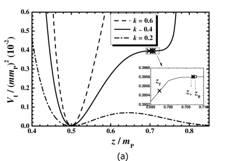
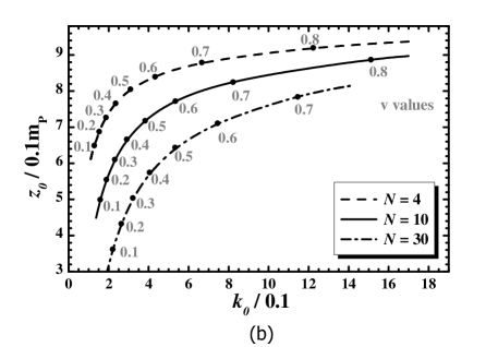
Figure 2: (a) Dimensionless inflationary potential $V_{\rm I}/m^{2}m_{\rm P}^{2}$ as a function of $z$ for $k=0.40167291$ (black line) or $k=0.2$ (dot-dashed line) or $k=0.6$ (dashed line) and the remaining inputs in Fig. 1. The values of $z_{\star}$, $z_{\rm f}$ and $z_{0}$ (for the first case) are also indicated. (b) Location of the inflection point in the $k_{0}-z_{0}$ plane for various $N$’s indicated in the plot. Shown is also the variation of ${\rm v}$ in gray along the lines.

5.2 Approaching the Inflationary Dynamics

Due to the complicate form of $V_{\rm I}$ in Eq. (29), we limit ourselves in expanding numerically $V_{\rm I}$ and $J$ about $z=z_{0}$ with results

$$V_{\rm I}\simeq v_{0}+v_{1}\delta z+v_{2}\delta z^{2}+v_{3}\delta z^{3}\>\>\mbox{and}\>\>J\simeq J_{0},\>\>\mbox{where $\delta z=z-z_{0}$, $v_{0}=V_{\rm I}(z_{0})$ and $J_{0}=J(z_{0})$}$$ (31)

For the inputs in Fig. 1 the expansion parameters above are given in Table 5. The relevant coefficients depend on the selected parameters ${\rm v},N,k,z_{0}$ and $\delta k$. Since $v_{1}=V_{\rm I}^{\prime}(z_{0})$ and $v_{2}=V_{\rm I}^{\prime\prime}(z_{0})/2\ll v_{0},v_{3}$ we neglect henceforth terms with $v_{1}^{2},v_{2}^{2}$ and $v_{1}v_{2}$.

$v_{0}/(mm_{\rm P})^{2}$	$v_{1}/(mm_{\rm P})^{2}$	$v_{2}/(mm_{\rm P})^{2}$	$v_{3}/(mm_{\rm P})^{2}$	$J_{0}$
$3.9\cdot 10^{-3}$	$1.5\cdot 10^{-6}$	$-2.1\cdot 10^{-6}$	$2.2$	$5.4$

Table 5: Expansion parameters for the inputs in Fig. 1.

Taking as inputs the parameters above we can investigate the inflationary evolution by estimating:

(a) The slow-roll parameters.

They are found to be

$$\epsilon=\left(\frac{V_{{\rm I},\widehat{z}}}{\sqrt{2}V_{{\rm I}}}\right)^{2}\simeq\frac{v_{1}+\delta z(2v_{2}+3\delta zv_{3})}{\sqrt{2}J_{0}v_{0}}~{}~{}\mbox{and}~{}~{}\eta=\frac{V_{{\rm I},\widehat{z}\widehat{z}}}{V_{\rm I}}\simeq\frac{2(v_{2}+3\delta zv_{3})}{J_{0}^{2}v_{0}}\,.$$ (32)

The realization of IPI is delimited by the condition

$${\footnotesize\sf max}\{\epsilon(\widehat{z}),|\eta(\widehat{z})|\}\leq 1,$$ (33)

which is saturated for $\delta z=\delta z_{\rm f}$ found as follows

$$\eta\left(\delta z_{\rm f}\right)\simeq 1~{}~{}\Rightarrow~{}~{}\delta z_{\rm f}\simeq-(J_{0}^{2}v_{0}+2v_{2})/6v_{3}<0.$$ (34)

Given that $J_{0}^{2}v_{0}\gg v_{2}$, we expect $\delta z_{\rm f}<0$ or $z_{\rm f}<z_{\star}$.

(b) The number of e-foldings ${N_{\star}}$ that the scale $k_{\star}=0.05/{\rm Mpc}$ experiences during IPI.

It is estimated to be

$${N_{\star}}=\int_{\widehat{z}_{\rm f}}^{\widehat{z}_{\star}}d\widehat{z}\frac{V_{\rm I}}{V_{{\rm I},\widehat{z}}}=\frac{f_{N\star}-f_{N{\rm f}}}{p_{N}}~{}~{}\mbox{where}~{}~{}p_{N}=\frac{\sqrt{3v_{1}v_{3}}}{J_{0}^{2}v_{0}}\>\>\mbox{and}\>\>f_{N}(z)=\arctan\frac{v_{2}+3zv_{3}}{\sqrt{3v_{1}v_{3}}}.$$ (35)

Also $z_{\star}~{}[\widehat{z}_{\star}]$ is the value of $z~{}[\widehat{z}]$ when $k_{\star}$ crosses the inflationary horizon and we define $f_{N\star}=f_{N}(\delta z_{\star})$ and $f_{N{\rm f}}=f_{N}(\delta z_{\rm f})$. Solving it w.r.t $\delta z_{\star}$ we obtain

$$\delta z_{\star}\simeq-\frac{v_{2}}{3v_{3}}+\sqrt{\frac{v_{1}}{3v_{3}}}\tan\left(\frac{\sqrt{3}{N_{\star}}}{J_{0}^{2}v_{0}}+f_{N{\rm f}}\right)<0~{}~{}\Rightarrow~{}~{}z_{\star}<z_{0}.~{}~{}$$ (36)

Therefore, we have no ultra slow roll for $z_{\rm f}\leq z\leq z_{\star}$. Note that ${N_{\star}}$, has to be sufficient to resolve the horizon and flatness problems of standard big bang [4] i.e.

$${N_{\star}}\simeq 61+\ln\left(\pi v_{0}T_{\rm rh}^{2}\right)^{1/6},$$ (37)

where $T_{\rm rh}$ is the reheating temperature – see below.

(c) The amplitude $A_{\rm s}$ of the power spectrum of the curvature perturbations.

Taking into account also the normalization of $A_{\rm s}$ [4] we achieve a prediction for the $m$ value. Indeed,

$$A_{\rm s}^{1/2}=\frac{1}{2\sqrt{3}\,\pi}\;\frac{V_{\rm I}^{3/2}(\widehat{z}_{\star})}{\left|V_{\rm I,\widehat{z}}(\widehat{z}_{\star})\right|}\simeq\frac{J_{0}v_{0}^{3/2}}{2\sqrt{3}\pi v_{1}}\cos^{2}\left(p_{N}{N_{\star}}+f_{N{\rm f}}\right)\simeq 4.588\cdot 10^{-5}~{}~{}\Rightarrow~{}~{}m\sim 10^{-7}m_{\rm P}.$$ (38)

(d) The remaining inflationary observables.

Namely, for the spectral index $n_{\rm s}$, its running, $a_{\rm s}$, and the tensor-to-scalar ratio $r$ we obtain

$$n_{\rm s}=\>1-6\epsilon_{\star}\ +\ 2\eta_{\star}\simeq 1+4p_{N}\tan\left(p_{N}{N_{\star}}+f_{N{\rm f}}\right),\>\>r=16\epsilon_{\star}\simeq 8v_{1}^{2}\cos^{-4}\left(p_{N}{N_{\star}}+f_{N{\rm f}}\right)/J_{0}^{2}v_{0}^{2},~{}~{}~{}~{}$$ (39a)

$$a_{\rm s}=\>2\left(4\eta_{\star}^{2}-(n_{\rm s}-1)^{2}\right)/3-2\xi_{\star}\simeq-4p_{N}\cos^{-2}\left(p_{N}{N_{\star}}+f_{N{\rm f}}\right)\>\>\mbox{with}\>\>\xi={V_{{\rm I},\widehat{}z}V_{{\rm I},\widehat{}z\widehat{}z\widehat{}z}/V^{2}_{\rm I}}.$$ (39b)

Here the variables with subscript $\star$ are evaluated at $z=z_{\star}$. Note that the combined Bicep2/Keck Array [6] and Planck data (fitted with the $\Lambda$CDM$+r+a_{\rm s}$ model) require [5]

$$n_{\rm s}=0.9658\pm 0.008,\>a_{\rm s}=-0.0066\pm 0.014\>\>\mbox{and}\>\>r\lesssim 0.068~{}~{}\mbox{at 95\% c.l.}$$ (40)

For the inputs of Fig. 1 we present some values of the inflationary parameters in Table 6 which turn out to be consistent with Eq. (40). From the values accumulated there, we observe that the results of our semianalytic approach – displayed in curly brackets – are quite close to the numerical ones. The semiclassical approximation, used in our analysis, is perfectly valid since $V_{\rm I\star}^{1/4}\ll m_{\rm P}$. The $\theta=0$ direction is well stabilized and does not contribute to the curvature perturbation, since for the relevant effective mass $m_{\theta\rm I}$ we find $m^{2}_{\theta\rm I}>0$ for $N>3$ and $m_{\theta\rm I\star}/H_{\rm I\star}>1$ where $H_{\rm I}=(V_{\rm I}/3)^{1/2}$. The one-loop radiative corrections, $\Delta\widehat{V}_{\rm I}$, to $V_{\rm I}$ induced by $m_{\theta\rm I}$ let intact our inflationary outputs.

$k_{0}/0.1$	$z_{0}/0.1m_{\rm P}$	$\delta k/10^{-6}$	$\delta z_{\star}/10^{-4}m_{\rm P}$
$4.0166971$	$7.07433$	$3.20232$	$-1.5$ {$-1.1$}
$V_{\rm I\star}^{1/4}/{\mbox{\rm EeV}}$	$H_{\rm I\star}/{\mbox{\rm EeV}}$	$\delta z_{\rm f}/10^{-2}m_{\rm P}$		$m_{\theta\rm I\star}/H_{\rm I\star}$
$4.6\cdot 10^{5}$	$49.5$	$-1.16$ {$-0.87$}		$5.1$
$n_{\rm s}$	$r/10^{-8}$	$-a_{\rm s}/10^{-3}$	$10^{5}A_{\rm s}^{1/2}$	${N_{\star}}$
$0.966$ {$0.97$}	$4.8$ {$3.9$}	$3.3$ {$3.2$}	$4.59$ {$4.27$}	$46.5$ {$45$}

Table 6: Sample values of inflationary parameters for the inputs in Fig. 1.

5.3 Inflaton Decay and Reheating

Soon after the end of IPI, the (canonically normalized) sgoldstino

$$\widehat{\updelta z}=\langle{J}\rangle{\updelta}z~{}~{}\mbox{with}~{}~{}{\updelta}z=z-{\rm v}~{}~{}\mbox{and}~{}~{}\langle{J}\rangle=\sqrt{\frac{N}{2}}\frac{1}{\langle{\omega}\rangle}$$ (41)

settles into a phase of damped oscillations abound the minimum reheating the universe at a temperature

$$T_{\rm rh}=\left({72/5\pi^{2}g_{\rm rh*}}\right)^{1/4}{\Gamma}_{{\updelta}z}^{1/2}m_{\rm P}^{1/2}\>\>\mbox{where $g_{\rm rh*}=106.75$ and}\>\>\>{\Gamma}_{{\updelta}z}\simeq{\Gamma}_{3/2}+{\Gamma}_{\theta}+{\Gamma}_{\tilde{h}}$$ (42)

the total decay width, ${\Gamma}_{{\updelta}z}$, of $\widehat{\updelta z}$ with the individual decay widths are found to be

$${\Gamma}_{3/2}\simeq\frac{\langle{\omega}\rangle^{-\sqrt{3N}}m_{z}^{5}}{96\pi m^{2}m_{\rm P}^{2}},~{}~{}{\Gamma}_{\theta}\simeq\frac{m_{z}^{3}}{16N\pi{\rm v}m_{\rm P}}~{}~{}\mbox{and}~{}~{}{\Gamma}_{\tilde{h}}=\frac{N\widehat{\mu}^{2}}{16\pi m_{\rm P}^{2}}m_{z}\,.$$ (43)

They express decay of $\widehat{\updelta z}$ into gravitinos, pseudo-sgoldstinos and higgsinos via the $\mu$ term respectively. Note that ${\Gamma}_{\tilde{h}}$ becomes rather enhanced for large $N$’s. Thanks to the high $m_{z}$ and $\widehat{\mu}$ values, no moduli problem arises in this context since $T_{\rm rh}\sim 1~{}{\mbox{\rm PeV}}\gg 1~{}{\rm MeV}$.

6 Results

The free parameters of the model are

$$m,N,{\rm v},\delta k=k-k_{0}~{}~{}\mbox{and}~{}~{}\delta z_{\star}=z_{\star}-z_{0}$$

Recall that $(k_{0},z_{0})$ is the inflection point which can be computed self-consistently for any selected $N$ and ${\rm v}$. Enforcing Eqs. (37) and (38) we restrict $\delta k$ and $m$ whereas the $n_{\rm s}$ bounds in Eq. (40) determines $\delta z_{\star}$. Increasing $\delta k$ allows us to increase the slope of the plateau around $z_{0}$ decreasing, thereby, ${N_{\star}}$. The model’s predictions regard $a_{\rm s}$ and $r$ estimated from Eq. (39b).

The outputs of our numerical investigation are presented:

(a) In Fig. 3, where we plot allowed domains in the $\delta k-(-\delta z_{\star})$ plane.

In Fig. 3-(a) we fix $N$ to three representative values $4,10$ and $30$ and display the allowed curves (dot-dashed, solid and dashed lines respectively) taking the central $n_{\rm s}$ value in Eq. (40). The variation of ${\rm v}$ along each line is displayed in gray. On the other hand, in Fig. 3-(b) we set ${\rm v}=0.5$ and identify the allowed (shaded) region by varying $n_{\rm s}$ in the margin of Eq. (40). The variation of $N$ is shown along each line. Besides the bounds on $n_{\rm s}$ in Eq. (40), which yield the dashed and dot-dashed lines, we take into account the upper bound in Eq. (28) which is saturated along the dotted line and the lower bound on $N$, mentioned above Eq. (21), along the double dotted dashed line. We remark that increasing $|\delta z_{\star}|$, decreases $n_{\rm s}$ with fixed $\delta k$. For $N=10$ and central $n_{\rm s}$ in Eq. (40) the inflationary predictions are

$$a_{\rm s}\simeq-3\cdot 10^{-3}\>\>\>\mbox{and}\>\>\>r\simeq 5\cdot 10^{-8}\>\>\>\mbox{for}\>\>\>T_{\rm rh}\simeq 1.75~{}{\mbox{\rm PeV}}\>\>\>\mbox{and}\>\>\>{N_{\star}}\simeq 46.5$$ (44)

The obtained $a_{\rm s}$ might be detectable in the future [17]. The needed tuning is of the order of $10^{-6}$ which is certainly ugly but milder than that needed for IPI within the conventional MSSM [14].

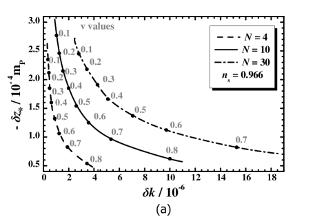
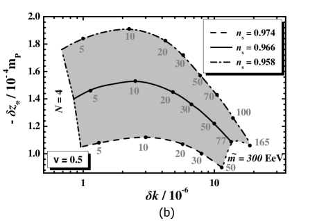
Figure 3: In the $\delta k-(-\delta z_{\star})$ plane we present (a) allowed curves for $n_{\rm s}\simeq 0.966$ and various $N$’s and (b) allowed (shaded) region varying continuously $N$. The variation of (a) ${\rm v}$ or (b) $N$ is shown in gray along the various lines. The constraint fulfilled along each line is shown in black.

(b) In Fig. 4, where we plot the mass spectrum as a function of $m$ for $n_{\rm s}\simeq 0.966$.

Namely, in Fig. 4-(a) we fix $N=10$ and vary ${\rm v}$ whereas in Fig. 4-(b) we fix ${\rm v}=0.5$ and vary $N$. The variation of the variable parameter is shown along the solid line in gray. The allowed values of $m_{3/2}$, $m_{z}$ and $m_{\theta}$, estimated by the expression in Eq. (21), are depicted by a solid, dashed and dot-dashed line respectively. From Fig. 4-(a) we remark that the hierarchy of the particle masses remains constant for fixed $N$. They remain of the order of $100~{}{\mbox{\rm EeV}}$ whereas $m$ becomes larger and larger than this level as ${\rm v}$ and/or $N$ increases. This is explained from Eq. (21) if we take into account that $\omega<1$ from Eq. (14) and $\sqrt{3N}/2>1$. In total we obtain

$$3\lesssim\frac{m}{1~{}{\mbox{\rm EeV}}}\lesssim 55600,~{}~{}0.89\lesssim\frac{m_{3/2}}{100~{}{\mbox{\rm EeV}}}\lesssim 3,\>\>2.3\lesssim\frac{m_{z}}{100~{}{\mbox{\rm EeV}}}\lesssim 4.4,~{}~{}\mbox{and}~{}~{}0.89\lesssim\frac{m_{\theta}}{100~{}{\mbox{\rm EeV}}}\lesssim 59.$$ (45)

This mass spectrum hints towards high-scale MSSM consistently with the LHC results on the Higgs boson mass – see Eq. (28). Needless to say, the stability of the electroweak vacuum up to $m_{\rm P}$ is automatically assured within this framework [18]. On the other hand, the gauge hierarchy problem becomes acute since the SUSY-mass scale is much higher than the electroweak scale and the relevant fine-tuning needed remains unexplained. From Fig. 4-(b) we also infer that the $\widehat{\updelta z}$ decay channel into $\theta$’s is kinematically blocked for $N\gtrsim 20$. We also find that for $N\lesssim 10$, ${\Gamma}_{{\updelta}z}\simeq{\Gamma}_{3/2}+{\Gamma}_{\tilde{h}}$ whereas for larger $N$’s ${\Gamma}_{{\updelta}z}\simeq{\Gamma}_{\tilde{h}}$ and so Eq. (42) yields $T_{\rm rh}\simeq(4-20)~{}{\mbox{\rm PeV}}$ resulting to ${N_{\star}}\simeq(45.5-46.7)$.

7 Conclusions

We proposed a SUGRA model with just one gauge-singlet chiral superfield (the Goldstino) that offers at once:

• Tiny cosmological constant in the low-energy vacuum at the cost of a fine tuned parameter;

• Inflection-point inflation resulting to an adjustable $n_{\rm s}$, a small $r$ and a sizable $a_{\rm s}\sim-10^{-3}$;

• Spontaneous SUSY breaking at the scale $\widetilde{m}\sim 100~{}{\mbox{\rm EeV}}$, which is consistent with the Higgs boson mass measured at LHC within high-scale SUSY.

It would be interesting to investigate the following issues:

• The generation of primordial black holes, which is currently under debate [24, 25] during an ultra slow-roll phase. Here we did not address the question of how $z$ reaches $z_{0}$. Since $z_{\star}<z_{0}$, we assumed that the slow-roll approximation offers a reliable description of IPI. This is true if $z$ lies initially near $z_{0}$ with a small enough kinetic energy density [23].

• The candidacy of intermediate-scale lightest neutralino with mass $M_{1}\sim{\mbox{\rm EeV}}$ in the interval $T_{\rm rh}<M_{1}<T_{\rm max}$ as a cold dark matter candidate adapting the production mechanism of WIMPZILLAS [26].

• The realization baryogenesis via non-thermal leptogenesis taking into account similar attempts – see e.g. Ref. [27].

• The reconciliation of our proposal with swampland conjectures [28] – see e.g. Ref. [29] for relevant modifications which may render our setting more friendly with the string ultraviolet completions.

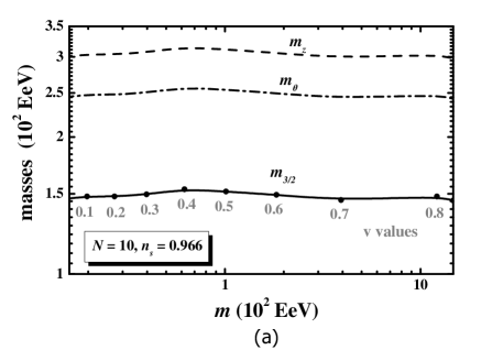
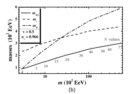
Figure 4: Allowed values of $m_{3/2}$, $m_{z}$ and $m_{\theta}$ (solid, dashed and dot-dashed line respectively) versus $m$ for $n_{\rm s}\simeq 0.966$ and (a) $N=10$ or (b) ${\rm v}=0.5$. The variation of ${\rm v}$ (a) or (b) $N$ is shown along the solid line in gray.

Acknowledgments

I would like to thank S. Ketov and M. Saridakis and for interesting discussions. This research work was supported by the Hellenic Foundation for Research and Innovation (H.F.R.I.) under the “First Call for H.F.R.I. Research Projects to support Faculty members and Researchers and the procurement of high-cost research equipment grant” (Project Number: 2251).

References

- [1] J. Ellis, B. Nagaraj, D.V. Nanopoulos and K.A. Olive, De Sitter Vacua in No-Scale Supergravity, J. High Energy Phys. 11, 110 (2018) [arXiv:1809.10114]; J. Ellis, B. Nagaraj, D.V. Nanopoulos, K.A. Olive and S. Verner, From Minkowski to de Sitter in Multifield No-Scale Models, J. High Energy Phys. 10, 161 (2019) [arXiv:1907.09123].
- [2] C. Pallis, From Minkowski to de Sitter Vacua with Various Geometries, Eur. Phys. J. C 83, no. 4, 328 (2023) [arXiv:2211.05067].
- [3] C. Pallis, Inflection-point sgoldstino inflation in no-scale supergravity, Phys. Lett. B 843, 138018 (2023) [arXiv:2302.12214].
- [4] N. Aghanim et al. [Planck Collaboration], Planck 2018 results. VI. Cosmological parameters, Astron. Astrophys. 641, A6 (2020) [arXiv:1807.06209].
- [5] Y. Akrami et al. [Planck Collaboration], Planck 2018 results. X. Constraints on inflation, Astron. Astrophys. 641, A10 (2020) [arXiv:1807.06211].
- [6] P.A.R. Ade et al., BICEP2 / Keck Array x: Constraints on Primordial Gravitational Waves using Planck, WMAP, and New BICEP2/Keck Observations through the 2015 Season, Phys. Rev. Lett. 121, 221301 (2018) [arXiv:1810.05216].
- [7] J. Polonyi, Generalization of the massive scalar multiplet coupling to the supergravity, Budapest preprint KFKI/1977/93 (1977).
- [8] M. Claudson, L. Hall and I. Hinchliffe, Tuning the cosmological constant in N=1 supergravity with an symmetry, Phys. Lett. B 130, 260 (1983).
- [9] S. Kachru, R. Kallosh, A.D. Linde and S. P. Trivedi, De Sitter vacua in string theory, Phys. Rev. D 68, 046005 (2003) [hep-th/0301240].
- [10] C. Pallis, Gravity-mediated SUSY breaking, R symmetry, and hyperbolic Kähler geometry, Phys. Rev. D 100, no. 5, 055013 (2019) [arXiv:1812.10284]; C. Pallis, SUSY-breaking scenarios with a mildly violated symmetry, Eur. Phys. J. C 81, no. 9, 804 (2021) [arXiv:2007.06012].
- [11] J. Ellis, M.A.G. Garcia, N. Nagata, D.V. Nanopoulos, K.A. Olive and S. Verner, Building models of inflation in no-scale supergravity, Int. J. Mod. Phys. D 29, 16, 2030011 (2020) [arXiv:2009.01709].
- [12] G. ’t Hooft, Naturalness, chiral symmetry, and spontaneous chiral symmetry breaking, NATO Sci. Ser. B 59, 135 (1980).
- [13] R. Kallosh and A. Linde, Planck, LHC and -attractors, Phys. Rev. D 91, 083528 (2015) [arXiv:1502.07733]; M.C. Romão and S.F. King, Starobinsky-like inflation in no-scale supergravity Wess-Zumino model with Polonyi term J. High Energy Phys. 07, 033 (2017) [arXiv:1703.08333]; K. Harigaya and K. Schmitz, Inflation from High-Scale Supersymmetry Breaking, Phys. Lett. B 773, 320 (2017) [arXiv:1707.03646]; I. Antoniadis, A. Chatrabhuti, H. Isono and R. Knoops, Inflation from Supersymmetry Breaking, Eur. Phys. J. C 77, no. 11, 724 (2017) [arXiv:1706.04133]; E. Dudas, T. Gherghetta, Y. Mambrini and K.A. Olive, Inflation and High-Scale Supersymmetry with an EeV Gravitino, Phys. Rev. D 96, no. 11, 115032 (2017) [arXiv:1710.07341]; Y. Aldabergenov, A. Chatrabhuti and H. Isono, -attractors from supersymmetry breaking, Eur. Phys. J. C 81, no. 2, 166 (2021) [arXiv:2009.02203].
- [14] R. Allahverdi, K. Enqvist, J. Garcia-Bellido and A. Mazumdar, Inflection point inflation within supersymmetry, Phys. Rev. Lett. 97, 191304 (2006) [hep-ph/0605035]; J.C. Bueno Sanchez, K. Dimopoulos and D.H. Lyth, A-term inflation and the MSSM, J. Cosmol. Astropart. Phys. 01, 015 (2007) [hep-ph/0608299].
- [15] S.-M. Choi and H.M. Lee, Inflection point inflation and reheating, Eur. Phys. J. C 76 303, no. 6 (2016) [arXiv:1601.05979]; M. Drees and Y. Xu, Small field polynomial inflation: reheating, radiative stability and lower bound, J. Cosmol. Astropart. Phys. 09, 012 (2021) [arXiv:2104.03977].
- [16] C. Pallis, An alternative framework for E-model inflation in supergravity, Eur. Phys. J. C 82, no. 5, 444 (2022) [arXiv:2204.01047].
- [17] J.B. Muñoz et al., Towards a measurement of the spectral runnings, J. Cosmol. Astropart. Phys. 05, 032 (2017) [arXiv:1611.05883].
- [18] E. Bagnaschi, G.F. Giudice, P. Slavich and A. Strumia, Higgs Mass and Unnatural Supersymmetry, J. High Energy Phys. 09, 092 (2014) [arXiv:1407.4081].
- [19] A. Brignole, L.E. Ibáñez and C. Muñoz, Soft supersymmetry breaking terms from supergravity and superstring models, Adv. Ser. Direct. High Energy Phys. 18, 125 (1998) [hep-ph/9707209].
- [20] C. Pallis, Kination-dominated reheating and cold dark matter abundance, Nucl. Phys. B751, 129 (2006) [hep-ph/0510234]; J. Ellis et al., BICEP/Keck constraints on attractor models of inflation and reheating, Phys. Rev. D 105, no.4, 043504 (2022) [arXiv:2112.04466].
- [21] M. Endo, F. Takahashi and T.T. Yanagida, Inflaton Decay in Supergravity, Phys. Rev. D 76, 083509 (2007) [arXiv:0706.0986]; J. Ellis, M. Garcia, D. Nanopoulos and K. Olive, Phenomenological Aspects of No-Scale Inflation Models, J. Cosmol. Astropart. Phys. 10, 003 (2015) [arXiv:1503.08867]; Y. Aldabergenov, I. Antoniadis, A. Chatrabhuti and H. Isono, Reheating after inflation by supersymmetry breaking, Eur. Phys. J. C 81, no. 12, 1078 (2021) [arXiv:2110.01347]; K.J. Bae, H. Baer, V. Barger and R.W. Deal, The cosmological moduli problem and naturalness, J. High Energy Phys. 02, 138 (2022) [arXiv:2201.06633].
- [22] J. Garcia-Bellido and E. Ruiz Morales, Primordial black holes from single field models of inflation, Phys. Dark Univ. 18, 47 (2017) [arXiv:1702.03901]; C. Germani and T. Prokopec, On primordial black holes from an inflection point, Phys. Dark Univ. 18, 6 (2017) [arXiv:1706.04226].
- [23] K. Dimopoulos, Ultra slow-roll inflation demystified, Phys. Lett. B775, 262 (2017)[arXiv:1707.05644].
- [24] J. Kristiano and J. Yokoyama, Ruling Out Primordial Black Hole Formation From Single-Field Inflation, arXiv:2211.03395.
- [25] H. Firouzjahi and A. Riotto, Primordial Black Holes and loops in single-field inflation, J. Cosmol. Astropart. Phys. 02, 021 (2024) [arXiv:2304.07801].
- [26] D.J.H. Chung, E.W. Kolb and A. Riotto, Nonthermal supermassive dark matter, Phys. Rev. Lett. 81, 4048 (1998) [hep-ph/9805473].
- [27] K. Kaneta, Y. Mambrini, K.A. Olive and S. Verner, Inflation and Leptogenesis in High-Scale Supersymmetry, Phys. Rev. D 101, no. 1, 015002 (2020) [arXiv:1911.02463].
- [28] C. Vafa, Distance and de Sitter conjectures on the swampland, hep-th/0509212.
- [29] I.M. Rasulian, M. Torabian and L. Velasco-Sevilla, Swampland de Sitter conjectures in no-scale supergravity models, Phys. Rev. D 104, no.4, 044028 (2021) [arXiv:2105.14501].