An extended Su-Schrieffer-Heeger model with time-reversal symmetry protection
Abstract
In this work, we theoretically study a modified Su-Schrieffer-Heeger (SSH) model in which each unit cell consists of three sites. Unlike existing extensions of the SSH model which are made by enlarging the periodicity of the (nearest-neighbor) hopping amplitudes, our modification is obtained by replacing the Pauli matrices in the system’s Hamiltonian by their higher dimensional counterparts. This in turn leads to the presence of next-nearest neighbor hopping terms and the emergence of different symmetries than those of other extended SSH models. Moreover, the system supports a number of edge states that are protected by the time-reversal symmetry rather than the usual chiral symmetry. Finally, our system could be potentially realized in various experimental platforms including superconducting circuits as well as acoustic/optical waveguide arrays.
I Introduction
In condensed matter physics, the topological features of matter have gained a lot of interest ever since topological insulators were discovered Kane2005 ; Konig2007 ; Hasan2010 . Topological insulators are peculiar types of materials that display an insulating bulk, as expected from insulating materials, but their edges are conducting. Due to these materials’ unique properties and potential applications, for example, in the field of quantum computing and spintronics He2022 ; He2019 ; Tokura2019 ; Fan2016 , topological insulators are still actively studied in the last few years Yang2023 ; Cai2023 ; Zhou2022 ; Denner2021 ; He2020 .
The Su-Schrieffer-Heeger (SSH) model Su1980 is the simplest and most fundamental model of topological insulators Asboth2016 . The SSH model describes a one-dimensional (1D) chain of unit cells, each of which contains two sites (dimers), and the coupling between intracell and intercell sites alternates. Two topologically distinct phases can be observed in the SSH structure. One of these phases, which is termed topologically nontrivial, is characterized by the presence of topologically protected zero-energy modes at the system’s two edges. Such edge modes are absent in the other phase, which is thus termed topologically trivial Asboth2016 . The SSH model has been thoroughly studied both experimentally and theoretically in various physical platforms, including photonics and optical systems On2024 ; Liang2023 ; Yu2022 ; Roberts2022 ; Henriques2022 ; Xu2022 , thermodynamic systems Upadhyay2024 ; Hao2022 , plasmonic systems Xia2023 ; Smith2021 ; Guan2021 ; Pocock2018 ; Downing2017 , ultracold atoms and gases Dong2024 ; L.Zhou2022 ; Jiang2022 ; Cooper2019 ; He2018 , ferromagnetic systems PT2022 ; Y.Li2021 , acoustic waveguide Guo2024 ; X.Yang2023 ; Q.Li2023 ; Coutant2022 ; Peng2018 , and superconducting systems Banerjee2023 ; Rosenberg2022 ; Wang2021 ; L.Qi2021 ; Rosenberg2021 and circuits Zhao2023 ; Zheng2022 ; Chen2022 . Due to its simplicity, the SSH model has further been the subject for the study of topological entanglement Navarro-Labastida2022 ; Fromholz2020 ; Micallo2020 . Finally, a creative use of the SSH model that illustrates quantum state transfer is revealed in Refs. Zurita2023 ; Chang2023 ; Zheng2023 ; C.Wang2022 ; Palaiodimopoulos2021 ; D'Angelis2020 ; Tan2020 ; Mei2018 .
In recent years, the SSH model has undergone a transformative extension, marked by the inclusion of long-range hopping parameters Cinnirella2024 ; Bera2023 ; Dias2022 ; Qi2021 ; Pérez-González2019 ; Li2015 , interaction effect Pan2024 ; T.Jin2023 ; Xing2023 ; Koor2022 ; Cai2022 ; Feng2022 ; Yu2020 , nonlinearity Jezequel2022 ; Y.Ma2021 ; Tuloup2020 , non-Hermiticity Lee2016 ; Yao2018 ; Okuma2023 , and/or periodic driving Asboth2014 ; Bomantara2019 ; Qiao2023 ; Wu2020 ; Pan2020 . Other extensions of the SSH model include the modifications of its unit cell to being trimer Verma2024 ; Anastasiadis2022 ; Alvarez2019 ; Du2024 or tetratomic Zhou2023 ; Marques2020 ; Xie2019 . Instead of adhering to conventional constraints of being the simplest topological insulator, such extended SSH models recognise the complexity of topological quantum phases and aim to uncover richer topological effects. This change in emphasis highlights the flexibility of the SSH model and its ability to deciphering the intricacies present in quantum processes across a wide range of physical systems. This in turn puts the family of extended SSH models at the forefront of theoretical and experimental investigation of exotic topological phases.
Our study investigates an extension of the SSH model by means of enlarging the unit cell to contain three sites (trimers). While a similar theme has been explored in previous studies such as Refs. Verma2024 ; Anastasiadis2022 ; Alvarez2019 ; Du2024 , we consider a totally different approach in developing our extended SSH model. That is, instead of considering three different nearest-neighbor hopping strengths, our model is obtained by replacing the Pauli matrices in the system’s Hamiltonian with their three-dimensional generalizations. As a result, our model also naturally incorporates some next-neighbor hopping terms. Due to this fundamental difference, our extended SSH model has different symmetries and topological properties from those of other trimer SSH models Verma2024 ; Anastasiadis2022 ; Alvarez2019 ; Du2024 . The extended SSH model we propose here features a number of edge states. Remarkably, these edge states persist despite the presence of time-reversal symmetry preserving perturbations, thus highlighting their topological nature. Finally, it is expected that our model could be experimentally implemented in various platforms that have been previously utilized to realize the SSH model. These include superconducting circuits Deng2022 ; Youssefi2022 ; Cai2019 and acoustic/optical waveguide arrays Cheng2019 ; Coutant2021 ; Yang2024 .
This paper is organized as follows. In Section II, we provide a detailed description of our model. There, we start by presenting the system’s Hamiltonian and elucidate its physical meaning. We then perform the momentum space analysis of the system to obtain the bulk band structure and uncover its four symmetries in II.1. In the same section, we also identify and calculate an appropriate topological invariant that dictates the system’s topology. We end the section with II.2 by analytically identifying the edge states at some special parameter values, then further supporting the findings by presenting the numerically obtained edge states at more general parameter values. In Sec. III.1, we briefly discuss the potential for realizing our system in experiments. We then consider four generic types of perturbations and investigate how they affect our model in Sec. III.2. In Section IV, we summarize our results and present potential aspects for future studies.
II Model description
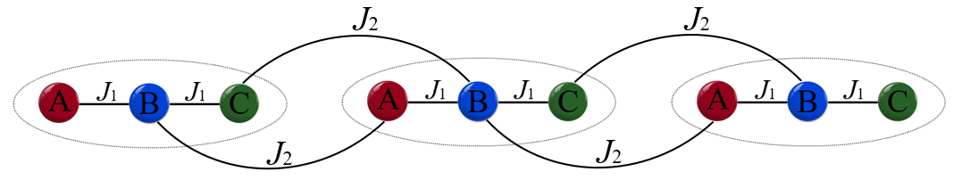
We consider an extended SSH model that has three sites per unit cell but only two coupling parameters; the coupling parameter controls the nearest-neighbor intracell hopping, while couples two neighboring unit cells (see Fig. 1). Mathematically, it is described by the Hamiltonian
| (1) |
where and are the creation and annihilation operators at sublattice of the unit cell, is the number of unit cells, and are the intracell and intercell hopping parameters, respectively.

II.1 Momentum space analysis
The origin of our model construction could be better understood by writing Eq. (1) in the momentum space, i.e.,
| (2) |
where , and are the higher dimention generalizations of Pauli matrices. It is worth noting that takes the same form as the momentum space Hamiltonian of the regular SSH model, but with the Pauli matrices and replaced by their three-dimensional counterparts. Our construction could then be, in principle, further generalized by replacing and by their -dimensional counterparts. However, we choose to focus on the case in this paper as the obtained model already exhibits rich topological effects.
Before presenting its spectral and topological features, we shall first identify the system’s symmetries. Specifically, we find that the system respects the chiral, time-reversal, particle-hole, and inversion symmetries. In terms of the momentum space Hamiltonian , there exists operators , , , and which respectively satisfy , , , and . These operators are explicitly given by , ( being the complex conjugation operator), , and . It is worth emphasizing that the above symmetries are different from those respected by other trimer SSH models previously studied in Refs. Verma2024 ; Anastasiadis2022 ; Alvarez2019 ; Du2024 . In particular, the models of Refs. Verma2024 ; Anastasiadis2022 ; Alvarez2019 do not have chiral symmetry, whereas the model of Ref. Du2024 lacks the particle-hole symmetry.
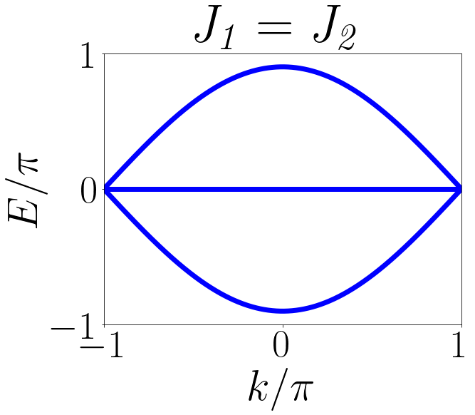
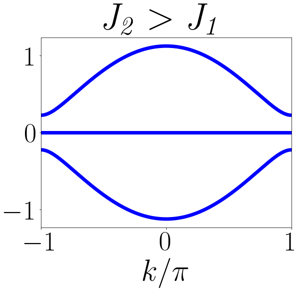
Due to the presence of chiral symmetry , the energy spectrum of our model is symmetrical about . Indeed, the eigenvalues of are calculated as follows,
| (3) |
These three bands are generically gapped (see Fig. 2), except at where they touch one another at the boundaries of the first Brillouin zone (). While the cases and appear to yield qualitatively similar spectral profiles, we will show in the following that they are topologically distinct. Moreover, our analysis in the next section further demonstrates the presence of edge states in the topologically nontrivial regime.
To unravel the topological origin of our model, we compute the normalized sublattice Zak’s phase, which was first introduced in Ref. Anastasiadis2022 , as
| (4) |
where is the eigenstate coresponding to , , and is the projector to sublattice , being an eigenstate of the chiral symmetry associated with the sublattice . As detailed in Appendix A, we find that
II.2 Formation of edge states in the real space
Having identified the band closing location, i.e., at , that separates the two distinct topological phases in the previous section we now turn our attention again to the real space description of Eq. (1). In particular, we aim to demonstrate the correlation between topology and the presence of edge states, i.e., the topologically nontrivial regime supports robust localized eigenstates near the system’s edges, whilst such edge states are absent in the topologically trivial regime .
We start by writing Eq. (1) under open boundary conditions in the form
| (5) |
where is a matrix of the form
| (6) |
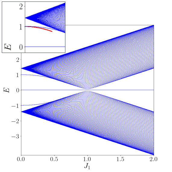
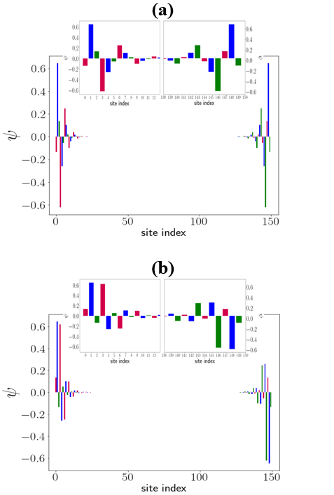
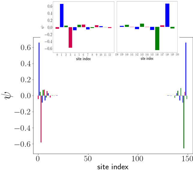
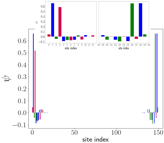
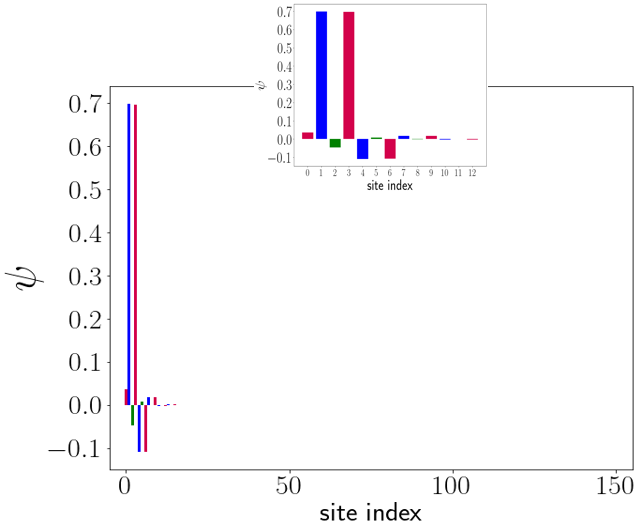
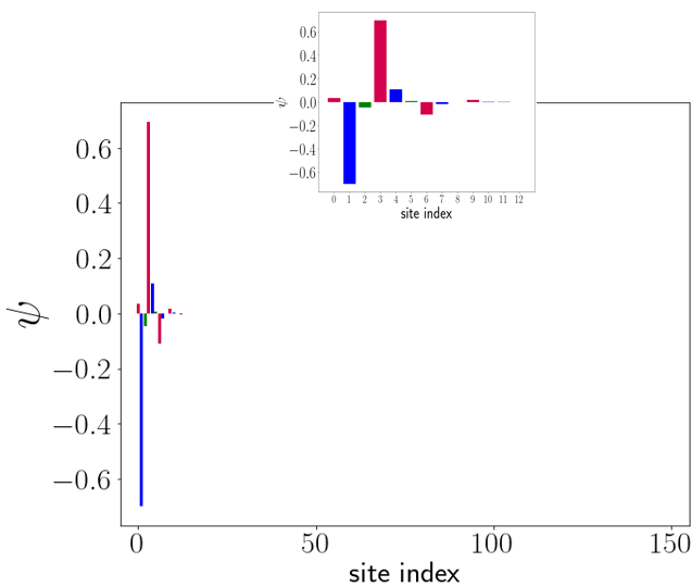
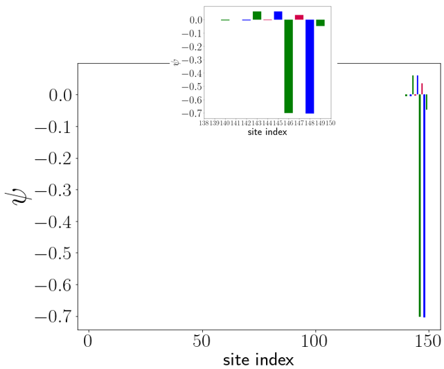
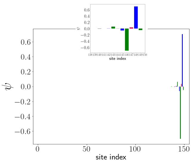
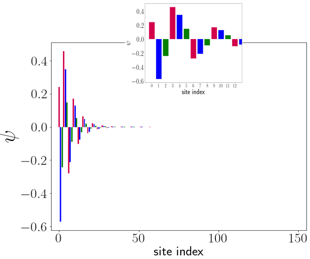
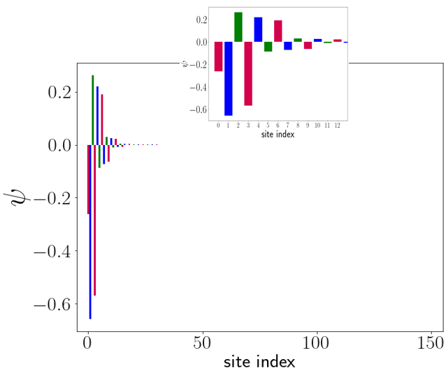
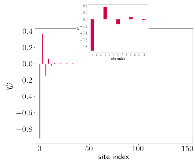
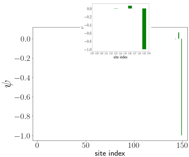
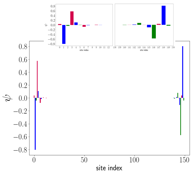
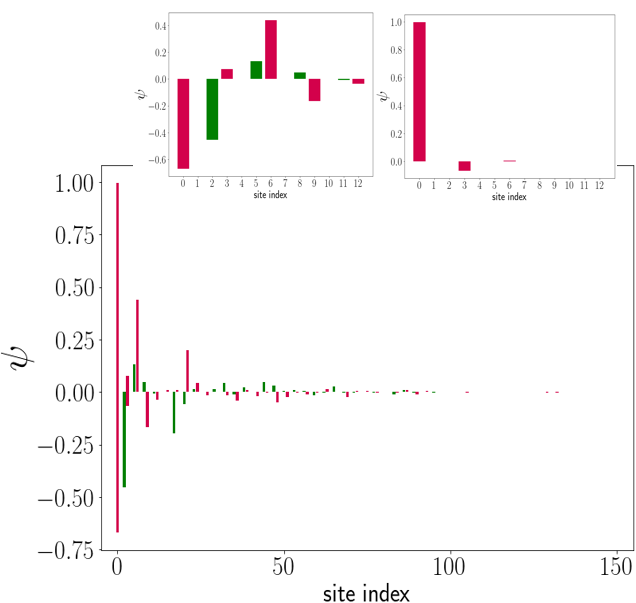
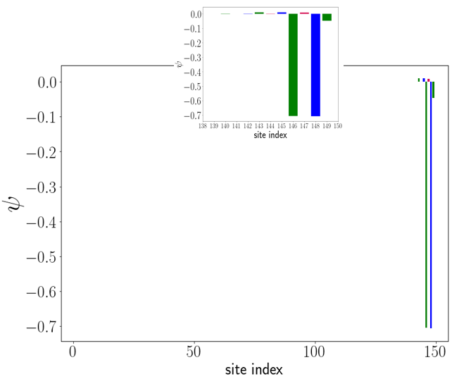
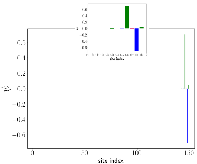
is a column vector whose elements are 1 at the th row ( for ) and 0 elsewhere. By numerically diagonalizing above, we obtain the system’s energy spectrum in Fig. 3. There, we verify that the bands are gapped, except at . Moreover, in-gap states are clearly observed in the regime , as we previously claimed. In Fig. 4, the wave function profiles of such in-gap states at fixed and values demonstrate their localized nature near the left or right end. This shows that, despite not being pinned at as in the regular SSH model, the observed in-gap states are in fact the sought after edge states. Upon closer inspection of Fig. 3, the energy of the observed edge states is quadratic with respect to and is exactly at . This insight allows us to support the above numerical results with an analytical treatment that will be discussed next.
To obtain the system’s edge states analytically, we start by setting and solve the eigenvalue equation with . By deferring the mathematical details to Appendix B, we obtain (ignoring any normalization constant)
for the left localized edge states and
for the right localized ones.
At nonzero values of , the energy of the edge states could be estimated via perturbation theory. In particular, by taking the intracell hopping term as the perturbative potential, i.e., , we find that the first-order energy correction for both edge states is . To obtain the lowest nonzero correction, we then evaluate the second-order correction as
| (7) | |||||
In the second equality above, we ignored all but one term in the summation. Specifically, we considered only the term coming from the other edge state localized in the same edge since it contains the largest overlap . Indeed, as demonstrated in the inset of Fig. 3, excellent agreement is observed between the analytically obtained edge state under second-order perturbative approximation above and the numerically obtained one.
III Discussion
III.1 Potential experimental realizations
Due to its simplicity, the regular SSH model has been realized in various experimental platforms, including superconducting circuits Deng2022 ; Youssefi2022 ; Cai2019 and acoustic/optical waveguide arrays Cheng2019 ; Coutant2021 ; Yang2024 . It is expected that, with suitable modifications, these experiments could be adapted to realize our extended SSH model.
The potentially nontrivial component of our extended SSH model that is not present in the regular SSH model is the next-nearest neighbor coupling, which necessarily arises due to the intercell hopping. Fortunately, such a next-nearest neighbor coupling could be handled in at least two different ways. First, specific to the optical waveguides platform, a next-nearest neighbor coupling could be achieved by using waveguide interference phenomena Savelev2020 . That is, we may efficiently link waveguides at extended distances by taking advantage of interference processes involving an extra supplemental waveguide in between. Alternatively, a potentially simpler means of handling the next-nearest neighbor couplings is by turning them into nearest neighbor ones. This could be achieved by rearranging the lattice configuration into a quasi-1D ladder as illustrated in Fig. 10.
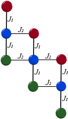
The extended SSH model under Fig. 10 configuration could be implemented in existing experimental platforms. For example, in superconducting circuits, the sites could represent Xmon qubits, whereas the coupling between two neighboring sites could be achieved inductively by a tunable coupler Mei2018 or capacitively such as in Cai2019 . In acoustic/optical waveguides, each lattice site is represented by a waveguide, the propagation direction of which simulates the arrow of time. In this case, the coupling between two neighboring waveguides is achieved by a tunneling effect that can be controlled by their separation XinLi2018 . The presence of edge states in the system could then be verified by exciting appropriate waveguides near a lattice edge and tracking the propagation dynamics.
III.2 Effects of perturbation
Topological edge states are particularly attractive for their robustness against perturbations that preserve the system’s protecting symmetries. In the following, we further support the topological signature of the system and identify its protecting symmetries by investigating the fate of its edge states in the presence of some representative perturbations. To this end, each of the following terms shall be separately added to the momentum space Hamiltonian of Eq. (2),
| , | |||||
| , | (8) |
where , , , and are the respective perturbation strengths. Under each of these perturbations, the respective real space Hamiltonian reads,
| (9) |
| (10) |
| (11) |
| (12) |
The perturbations and have the effect of introducing imbalance between the two intracell and intercell hopping amplitudes respectively. It is easily verified that both and preserve the chiral symmetry since and . In contrast to the perturbation which breaks time-reversal, particle-hole, and inversion symmetries, preserves time-reversal and particle-hole symmetries while breaking inversion symmetry.
The perturbation is chosen to introduce an on-site potential on sublattice , while at the same time further introducing imbalance between the two intracell hopping amplitudes. The perturbation is chosen to introduce on-site potentials on all three sublattices. Both and break the chiral and particle-hole symmetries while preserving time-reversal symmetry. On the other hand, the inversion symmetry is broken by and is preserved by .
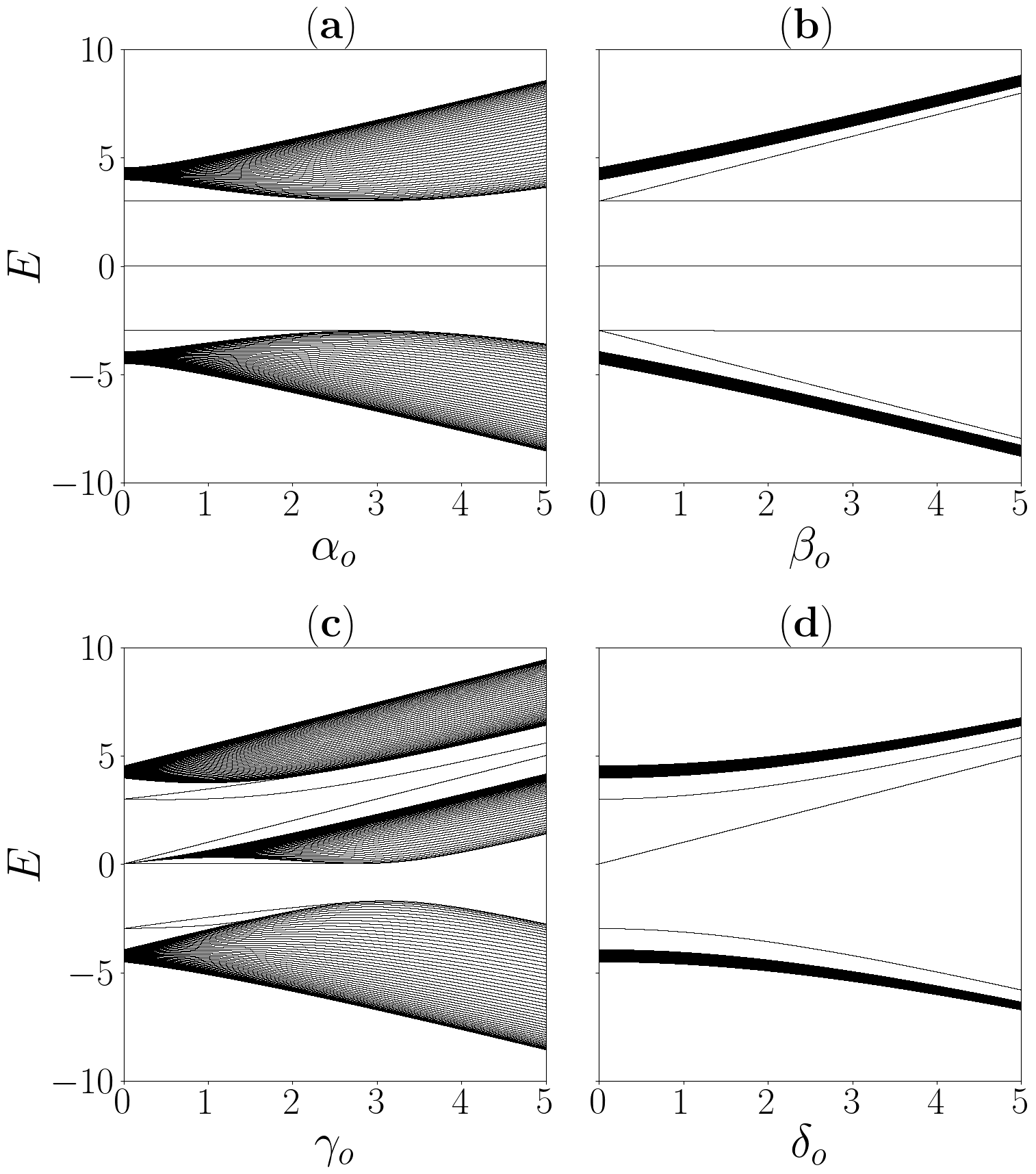
Figure 6 shows the energy spectra of our trimer SSH model in the presence of each of the aforementioned perturbations. As shown in Fig. 6(a), we find that the perturbation may lead to the disappearance of the edge states without being accompanied by band closing. On the other hand, Fig. 6(b-d) demonstrate that the other perturbations , , and merely modify the edge states structure but do not destroy them, even at considerably large values of , , and . Given that the time-reversal symmetry is the only symmetry that is simultaneously broken by and preserved by , , and , the above observations suggest that the system’s topology is protected by the time-reversal symmetry rather than the chiral symmetry as expected from the regular SSH model.
Note that the perturbations , , and have different effects on the edge states. Specifically, the perturbation breaks the degeneracy between the left and right edge states (see Fig. 6(b)). In this case, while the energy of the right edge states remains unaffected by the perturbation strength , the energy of the left edge states is shifted closer to the nearest bulk band. Consequently, at large enough , the left edge states merge with the bulk bands and disappear, whilst the right edge states remain present. Such an asymmetry between the number of edge states on the left and right edge states is unique to our extended SSH model and cannot be found in a regular SSH model (without breaking the sublattice degree of freedom). This phenomenon could be understood from Eq. (8) by observing that the perturbation only modifies the hopping involving sublattices A and B from two neighboring unit cells. As the left edge states have the largest support on sublattices A and B (see Fig. 4), they are signficantly affected by such a perturbation. By contrast, the right edges, which have the largest support on sublattices B and C (see Fig. 4), are much more insensitive to .
As the perturbation also modifies the hopping involving sublattices A and B while leaving the hopping involving sublattices B and C intact, the left and right edge states similarly develop an energy difference. Moreover, as the chiral symmetry is broken, there is further asymmetry between the positive and negative energies. In particular, as observed in Fig. 6(c), both the negative energy edge states eventually merge with the lower bulk band and disappear at large enough . On the other hand, at positive energy, only the right localized edge state merges with the upper bulk, whilst the left localized edge state persists even at very large . Interestingly, the perturbation also leads to new edge states emerging from the zero energy bulk states. One of these edge states, which is localized near the left edge, remains at zero energy and disappears at moderate after merging back with the center bulk band. The other, which is localized near the right edge, remains present at very large . It then follows that at , only two (almost degenerate) edge states at positive energy remain, one localized near the left edge whilst the other is localized near the right edge of the system.
Finally, the perturbation merely deforms the energy bands while leaving the edge states intact (see Fig. 6(d)). The breaking of the chiral symmetry again manifests itself as the asymmetry in the energy spectrum around that results from the center bulk band shifting upward. Nevertheless, the edge states remain well-gapped from the bulk bands even at large , thus ruling out the possibility for these edge states to merge with the bulk bands and disappear as in Fig. 6(a). This is consistent with the expectation that the system’s topology is protected by the time-reversal symmetry, which is preserved by . For completeness, in Appendix C, we show the wave function profiles of the various edge states under the different perturbations above.
IV Concluding remarks
We have presented a trimerized extension to the paradigmatic SSH model and uncovered its rich spectral and topological features. Unlike similar extensions proposed in existing literature, our model was obtained by replacing the sublattice Pauli matrices in the regular SSH model by their three-dimensional counterparts. Consequently, our trimer SSH models were shown to demonstrate fundamentally different edge state behaviors and symmetry protection. For example, our model possesses time reversal, chiral, particle-hole, and inversion symmetries. Moreover, in the topologically nontrivial regime, two pairs of edge states emerge symmetrically at positive and negative energies. In the presence of perturbations, such edge states remain robust provided the time-reversal symmetry is preserved.
Remarkably, some time-reversal preserving perturbations were found to destroy some existing edge states while at the same yielding new edge states. This in turn leads to an interesting scenario in which edge states are localized only on one edge of the system. Such a feature could find some useful application in the area of quantum communications, particularly related to the task of quantum state transfers Zurita2023 ; Chang2023 ; Zheng2023 ; C.Wang2022 ; Palaiodimopoulos2021 ; D'Angelis2020 ; Tan2020 ; Mei2018 . Indeed, transferring some quantum information from one edge of the lattice to the other could be accomplished by first encoding it in a subspace spanned by the vacuum state and the edge states (which are originally localized solely on one edge), then slowly transforming the system’s Hamiltonian into that which supports edge states solely on the other edge.
In the future, it would be worthwhile to extend our procedure for obtaining a family of extended SSH models with sites per unit cell. Such models are expected to exhibit even richer properties, the full analysis of which deserves a separate study. Another interesting direction to pursue is to investigate the effect of periodic driving to the present model. In particular, periodically driving a regular SSH model has already been shown to yield novel topological features with no static counterparts Q.Cheng2019 ; Z.Cheng2023 . It is thus envisioned that periodically driving our trimer SSH model will lead to more unexpected topological phenomena. Finally, non-Hermiticity Lee2016 ; Yao2018 ; Okuma2023 , nonlinearity Jezequel2022 ; Y.Ma2021 ; Tuloup2020 , and interaction effect Pan2024 ; T.Jin2023 ; Xing2023 ; Koor2022 ; Cai2022 ; Feng2022 ; Yu2020 are other aspects that could be considered to further enrich the physics of our model.
Acknowledgements.
This work was supported by the Deanship of Research Oversight and Coordination (DROC) at King Fahd University of Petroleum & Minerals (KFUPM) through project No. EC221010.Appendix A Detailed analytical calculation of the normalized sublattice Zak’s phase
Recall that the normalized sublattice Zak’s phase is given as
| (13) |
where
and the eigenstates for are
For the nonzero energies
the corresponding eigenstates are
It follows that
and
so that
and
Finally, straightforward calculation yields
Appendix B Detailed analytical calculation of the edge states at
By inspecting Fig. 3 in the main text, it is clear that at , the edge states correspond to energy . To analytically obtain the exact form of the edge states at this special parameter value, we thus attempt to solve
| (14) |
where Eq. (6) becomes (under ),
| (15) |
Using the same notation as that in Sec. II.2, we first write
| (16) |
By solving these equations:
The last two equations imply . Consequently, the only nonzero elements are . For , similar calculation yields and all other elements being zero. Plugging these results to Eq. (16), the left localized edge states are obtained as
By repeating the calculation above from going backward, we obtain similar expressions for the right localized edge states, i.e.,
Appendix C Wave function profiles of the edge states in the presence of perturbations
In the main text, we have demonstrated the robustness of the system’s edge states in the presence of time-reversal symmetry preserving perturbations. For completeness, we present in this section the wave function profiles corresponding to the surviving edge states under the perturbations considered in the main text. Our results are summarized in Figs. 7-11. Observe that in all cases, the edge states that originate from the unperturbed scenario (whose main peaks are at or ) remain present, thus demonstrating their robustness. One may notice that new edge state structures seemingly emerge in some cases (see Fig. 9 and Fig. 10). It is however worth emphasizing that the presence of such new edge states does not reflect a topological phase transition induced by the respective perturbations. In fact, these edge states are already present in the unperturbed case, which correspond to zero energy and thus coincide with the middle bulk band. In the presence of perturbation, these “newly formed” edge states remain at the same energy as the middle bulk band as evidenced in Fig. 10. On the other hand, in the presence of perturbation, such edge states are separated from the middle bulk band, increasing their visibility (see Fig. 9).


References
- (1) C. L. Kane and E. J. Mele, Phys. Rev. Lett. 95, 226801 (2005).
- (2) M. Koenig, S. Wiedmann, C. Brune, A. Roth, H. Buhmann, L. W. Molenkamp, X. Qi, and S. Zhang, Science 318, 766-770 (2007).
- (3) M. Z. Hasan and C. L. Kane, Rev. Mod. Phys. 82, 3045 (2010).
- (4) Q. L. He, T. L. Hughes, N. P. Armitage, Y. Tokura, and K. L. Wang, N. Materials 21, 15–23 (2022).
- (5) M. He, H. Sun, and Q. L. He, Front. Phys. 14, 43401 (2019).
- (6) Y. Tokura, K. Yasuda, and A. Tsukazaki, Nat. Rev. Phys. 1, 126–143 (2019).
- (7) Y. Fan and K. L. Wang, SPIN 6, 2 (2016).
- (8) Y. Yang, H. Sun, J. Lu, X. Huang, W. Deng, and Z. Liu, Communications Physics 6, 143 (2023).
- (9) L. Cai, R. Li, X. Wu, B. Huang, Y. Dai, and C. Niu, Phys. Rev. B 107, 245116 (2023).
- (10) L. Zhou, R. W. Bomantara, and S. Wu, SciPost Phys. 13, 015 (2022).
- (11) M. M. Denner, A. Skurativska, F. Schindler, M. H. Fischer, R. Thomale, T. Bzdušek, and T. Neupert, Nat. Commun. 12, 5681 (2021).
- (12) C. He, H. Lai, B. He, S. Yu, X. Xu, M. Lu, and Y. Chen, Nat. Commun. 11, 2318 (2020).
- (13) W. P. Su, J. R. Schrieffer, and A. J. Heeger, Phys. Rev. B 22, 2099 (1980).
- (14) J. K. Asbóth, L. Oroszlány, and A. Pályi, Lecture Notes in Physics 919, 166 (2016).
- (15) M. B. On, F. Ashtiani, D. Sanchez-Jacome, D. Perez-Lopez, S. J. B. Yoo, and A. Blanco-Redondo, Nat. Commun. 15, 629 (2024).
- (16) C. Liang, Y. Liu, F. Li, S. Leung, Y. Poo, and J. Jiang, Phys. Rev. Applied 20, 034028 (2023).
- (17) Z. Yu, H. Lin, R. Zhou, Z. Li, Z. Mao, K. Peng, Y. Liu, and X. Shi, J. Appl. Phys. 132, 163101 (2022).
- (18) N. Roberts, G. Baardink, J. Nunn, P. J. Mosley, and A. Souslov, Sci. Adv. 8, add3522 (2022).
- (19) J. C. G. Henriques, T. G. Rappoport, Y. V. Bludov, M. I. Vasilevskiy, and N. M. R. Peres, Phys. Rev. A 101, 043811 (2020).
- (20) X. Xu, Y. Zhao, H. Wang, A. Chen, and Y. Liu, Front. Phys. 9, 813801 (2022).
- (21) V. Upadhyay, M. T. Naseem, Ö. E. Müstecaplıoğlu, and R. Marathe, New J. Phys. 26, 013014 (2024).
- (22) H. Hao, S. Han, Y. Yang, D. Liu, H. Xue, G. Liu, Z. Cheng, B. Zhang, and Y. Luo, Adv. Mater. 34, 31 2202257 (2022).
- (23) S. Xia, D. Zhang, X. Zhai, L. Wang, and S. Wen, Appl. Phys. Lett. 123, 101102 (2023).
- (24) T. B. Smith, C. Kocabas, and A. Principi, J. Phys.: Condens. Matter 33, 265003 (2021).
- (25) Y. G., Z. Jiang, and S. Haas, Phys. Rev. B 104, 125425 (2021).
- (26) S. R. Pocock, X. Xiao, P. A. Huidobro, and V. Giannini, ACS Photonics 5(6), 2271–2279 (2018).
- (27) C. A. Downing and G. Weick, Phys. Rev. B 95, 125426 (2017).
- (28) Z. Dong, H. Li, T. Wan, Q. Liang, Z. Yang, and B. Yan, Nat. Photonics 18, 68–73 (2024).
- (29) L. Zhou, H. Li, W. Yi, and X. Cui, Commun. Phys. 5, 252 (2022).
- (30) J. Jiang, J. Zhang, F. Mei, Z. Ji, Y. Hu, J. Ma, L. Xiao, and S. Jia, Phys. Rev. A 106, 023318 (2022).
- (31) N. R. Cooper, J. Dalibard, and I. B. Spielman, Rev. Mod. Phys. 91, 015005 (2019).
- (32) Y. He, K. Wright, S. Kouachi, and C. Chien, Phys. Rev. A 97, 023618 (2018).
- (33) Peng-Tao Wei, Jin-Yu Ni, Xia-Ming Zheng, Da-Yong Liu, and Liang-Jian Zou, J. Phys. Condens. Matter 49, 34 (2022).
- (34) Y. Li and R. Cheng, Phys. Rev. B 103, 014407 (2021).
- (35) T. Guo, B. Assouar, B. Vincen, A. Merkel, J. Appl. Phys. 135, 043102 (2024).
- (36) X. Yang, H. Jia, P. Zhang, S. Wang, Y. Yang, Y. Yang, and X. Li, J. Appl. Phys. 133, 195104 (2023).
- (37) Q. Li, X. Xiang, L. Wang, Y. Huang, and X. Wu, Appl. Phys. Lett. 122, 191704 (2023).
- (38) A. Coutant, V. Achilleos, O. Richoux, G. Theocharis, and V. Pagneux, J. Acoust. Soc. Am. 151, 3626–3632 (2022).
- (39) Y. Peng, Z. Geng, and X. Zhu, J. Appl. Phys. 123, 091716 (2018).
- (40) D. Banerjee, J. Thomas, A. Nocera, and S. Johnston, Phys. Rev. B 107, 235113 (2023).
- (41) P. Rosenberg and E. Manousakis, Phys. Rev. B 106, 054511 (2022).
- (42) Z. Wang, F. Xu, L. Li, D. Xu, W. Chen, and B. Wang, Phys. Rev. B 103, 134507 (2021).
- (43) L. Qi, Y. Yan, Y. Xing, X. Zhao, S. Liu, W. Cui, X. Han, S. Zhang, and H. Wang, Phys. Rev. Research 3, 023037 (2021).
- (44) P. Rosenberg and E. Manousakis, Phys. Rev. B 104, 134511 (2021).
- (45) X. Zhao, Y. Xing, J. Cao, S. Liu, W. Cui, and H. Wang, npj Quantum Information 9, 59 (2023).
- (46) L. Zheng, X. Yi, and H. Wang, Phys. Rev. Applied 18, 054037 (2022).
- (47) J. Chen, C. Wu, J. Fan, and G. Chen, Chinese Phys. B 31, 088501 (2022).
- (48) L. A. Navarro-Labastida, F. A. Domınguez-Serna, and F. Rojas, Revista Mexicana de Fısica 68, 031404 (2022).
- (49) P. Fromholz, G. Magnifico, V. Vitale, T. Mendes-Santos, and M. Dalmonte, Phys. Rev. B 101, 085136 (2020).
- (50) T. Micallo, V. Vitale, M. Dalmonte, and P. Fromholz, SciPost Phys. Core 3, 012 (2020).
- (51) J. Zurita, C. E. Creffield, and G. Platero, Quantum 7, 1043 (2023).
- (52) Y. Chang, J. Xue, Y. Han, X. Wang, and H. Li, Phys. Rev. A 108, 062409 (2023).
- (53) L. Zheng, H. Wang, and X. Yi, New J. Phys. 25, 113003 (2023).
- (54) C. Wang, L. Li, J. Gong, and Y. Liu, Phys. Rev. A 106, 052411 (2022).
- (55) N. E. Palaiodimopoulos, I. Brouzos, F. K. Diakonos, and G. Theocharis, Phys. Rev. A 103, 052409 (2021).
- (56) F. M. D’Angelis, F. A. Pinheiro, D. Guéry-Odelin, S. Longhi, and François Impens, Phys. Rev. Research 2, 033475 (2020).
- (57) S. Tan, R. W. Bomantara, and J. Gong, Phys. Rev. A 102, 022608 (2020).
- (58) F. Mei, G. Chen, L. Tian, S. Zhu, and S. Jia, Phys. Rev. A 98, 012331 (2018).
- (59) E. G. Cinnirella, A. Nava, G. Campagnano, and D. Giuliano, Phys. Rev. B 109, 035114 (2024).
- (60) M. L. Bera, J. O. de Almeida, M. Dziurawiec, M. Płodzień, M. M. Maśka, M. Lewenstein, T. Grass, and U. Bhattacharya, Phys. Rev. B 108, 214104 (2023).
- (61) R. G. Dias and A. M. Marques, Phys. Rev. B 105, 035102 (2022).
- (62) L. Qi, Y. Yan, Y. Xing, X. Zhao, S. Liu, W. Cui, X. Han, S. Zhang, and Hong-Fu Wang, Phys. Rev. Research 3, 023037 (2021).
- (63) B. Pérez-González, M. Bello, Á. Gómez-León, and G. Platero, Phys. Rev. B 99, 035146 (2019).
- (64) L. Li, C. Yang, and S. Chen, Europhys. Lett., Volume 112, 10004 (2015).
- (65) H. Pan, Z. H. An, and C.-M. Hu, Phys. Rev. Research 6, 013020 (2024).
- (66) T. Jin, P. Ruggiero, and T. Giamarchi, Phys. Rev. B 107, L201111 (2023).
- (67) B. Xing, C. Feng, R. Scalettar, G. G. Batrouni, and D. Poletti, Phys. Rev. B 108, L161103 (2023).
- (68) K. Koor, R. W. Bomantara, and L. C. Kwek, Phys. Rev. B 106, 195122 (2022).
- (69) X. Cai, Z. Li, and H. Yao, Phys. Rev. B 106, L081115 (2022).
- (70) C. Feng, B. Xing, D. Poletti, R. Scalettar, and G. Batrouni, Phys. Rev. B 106, L081114 (2022).
- (71) X. Yu, L. Jiang, Y. Quan, T. Wu, Y. Chen, L. Zou, and J. Wu, Phys. Rev. B 101, 045422 (2020).
- (72) L. Jezequel and P. Delplace, Phys. Rev. B 105, 035410 (2022).
- (73) Y.-P. Ma and H. Susanto, Phys. Rev. E 104, 054206 (2021).
- (74) T. Tuloup, R. W. Bomantara, C. H. Lee, J. Gong, Phys. Rev. B 102, 115411 (2020).
- (75) T. E. Lee, Phys. Rev. Lett. 116, 133903 (2016).
- (76) S. Yao and Z. Wang, Phys. Rev. Lett. 121, 086803 (2018).
- (77) N. Okuma and M. Sato, Annu. Rev. Condens. Matter Phys. 14, 83-107 (2023).
- (78) J. K. Asboth, B. Tarasinski, P. Delplace, Phys. Rev. B 90, 125143 (2014).
- (79) R. W. Bomantara, L. Zhou, J. Pan, J. Gong, Phys. Rev. B 99, 045441 (2019).
- (80) Q. Qiao, L. Wang, G. Li, X. Chen, and L. Yuan, Nanophotonics vol. 12, pp. 3807-3815 (2023).
- (81) H. Wu and J. An, Phys. Rev. B 102, 041119(R) (2020).
- (82) Y. Pan and B. Wang, Phys. Rev. Research 2, 043239 (2020).
- (83) S. Verma and T. K. Ghosh. “Emergent SU(3) topological system in a trimer SSH model.” (2024).
- (84) L. A. Anastasiadis, G. Styliaris, R. Chaunsali, G. Theocharis, and F. K. Diakonos, Phys. Rev. B 106, 085109 (2022).
- (85) V. M. M. Alvarez and M. D. Coutinho-Filho, Phys. Rev. A 99, 013833 (2019).
- (86) T. Du, Y. Li, H. Lu, and H. Zhang, New J. Phys. 26, 023044 (2024).
- (87) X. Zhou, J. Pan, and S. Jia, Phys. Rev. B 107, 054105 (2023).
- (88) A. M. Marques and R. G. Dias, J. Phys. A: Math. Theor. 53, 075303 (2020).
- (89) D. Xie, W. Gou, T. Xiao, B.‘Gadway, and B. Yan, npj Quantum Information 5, 55 (2019).
- (90) J. Deng, H. Dong, C. Zhang, Y. Wu, J. Yuan, X. Zhu, F. Jin, H. Li, Z. Wang, H. Cai, C. Song, H.‘Wang, J. Q. You, and D. Wang, Science 378, 966-971 (2022).
- (91) A. Youssefi, S. Kono, A. Bancora, M. Chegnizadeh, J. Pan, T. Vovk, and T. J. Kippenberg, Nature 612, 666–672 (2022).
- (92) W. Cai, J. Han, F. Mei, Y. Xu, Y. Ma, X. Li, H. Wang, Y. P. Song, Z. Xue, Z. Yin, S. Jia, and L. Sun, Phys. Rev.‘Lett. 123, 080501 (2019).
- (93) Q. Cheng, Y. Pan, H. Wang, C. Zhang, D. Yu, A. Gover, H. Zhang, T. Li, L. Zhou, and S. Zhu, Phys. Rev. Lett. 122, 173901 (2019).
- (94) A. Coutant, A. Sivadon, L. Zheng, V. Achilleos, O. Richoux, G. Theocharis, V. Pagneux, Phys. Rev. B 103, 224309 (2021).
- (95) Y. Yang, R. J. Chapman, B. Haylock, F. Lenzini, Y. N. Joglekar, M. Lobino, and A. Peruzzo, Nat. Commun. 15, 50 (2024).
- (96) R. S. Savelev and M. A. Gorlach, Phys. Rev. B 102, 161112(R) (2020).
- (97) X. Li, Y. Meng, X. Wu, S. Yan, Y. Huang, S. Wang, and W. Wen, Appl. Phys. Lett. 113, 203501 (2018).
- (98) Q. Cheng, Y. Pan, H. Wang, C. Zhang, D. Yu, A. Gover, H. Zhang, T. Li, L. Zhou, and S. Zhu, Phys. Rev. Lett. 122, 173901 (2019).
- (99) Z. Cheng, R. W. Bomantara, H. Xue, W. Zhu, J. Gong, and B. Zhang, Phys. Rev. Lett. 129, 254301 (2023).