On the use of complex GTOs for the evaluation of radial integrals involving oscillating functions
Abstract
We study two classes of radial integrals involving a product of bound and continuum one-electron states. Using a representation of the continuum part with an expansion on complex Gaussian Type Orbitals, such integrals can be performed analytically. We investigate the reliability of this scheme for low-energy physical parameters. This study serves as a premise in view of potential applications in molecular scattering processes.
keywords:
Molecular integrals, complex Gaussians, continuum states- TDCS
- Triple Differential Cross Section
- STOs
- Slater Type Orbitals
- GTOs
- Gaussian Type Orbitals
- cGTOs
- complex Gaussian Type Orbitals
- rGTOs
- real Gaussian Type Orbitals
- FBA
- First Born Approximation
1 Introduction
The evaluation of integrals is a key issue in many atomic and molecular physics applications. Multicenter molecular integrals involving one or more electrons bound states are ubiquitous and essential in quantum chemistry calculations. The literature on the subject is abundant whether the bound functions involved are represented in terms of Slater Type Orbitals (STOs) or Gaussian Type Orbitals (GTOs). The latter have become particularly popular because a number of mathematical properties allows an efficient evaluation of multielectron bound states integrals [1, 2].
When one or several electrons are in a continuum state, the integrals are more difficult and the integration tools developed for bound states are not necessarily adapted, especially in the molecular case. The present manuscript is dedicated to a class of integrals involving products of one-electron bound and continuum states. An analytical approach based on a complex Gaussian Type Orbitals (cGTOs) representation of the continuum is proposed and its reliability is numerically investigated. While the ultimate goal would be to reach an all-Gaussian approach to evaluate the required multicentric and multielectrons integrals involved in scattering processes, we start here with a monocentric study and one-electron functions. The present work aims to better grasp the potential, the numerical efficiency and the range of applicability of the proposed strategy.
In the study of the ionization of atoms or molecules by a projectile, an electron () initially in a bound state is ejected into a continuum state with a given momentum . To calculate measurable quantities such as cross sections, within the first Born approximation one encounters the following matrix element (see, e.g., [3]):
| (1) |
where is the momentum transferred to the target by the projectile. For simplicity, here both electronic wave functions are written in a one-center description. One also encounters the case , that is to say the overlap which should vanish if the initial and final states are exact solutions of the same Hamiltonian. However, this is rarely the case since the two wave functions are usually calculated with different methods and making different approximations.
The factor recalls obviously also the Fourier transform. Since some seminal papers such as [4, 5], the Fourier transform method has been widely used in quantum chemistry. The integrals that appear, though, involve only bound states. Should Fourier transform techniques be envisaged for applications in which a combination of bound and continuum states is involved, matrix elements such as (1) would appear.
By using the Rayleigh expansion for and the standard expansions in spherical coordinates for the initial and final states, the angular integrations can be treated separately and performed analytically. One is thus left with the evaluation of radial integrals which is a challenge because the integrand oscillates up to large distances.
The purpose of this manuscript is twofold. First, we wish to explore numerical issues related to the different parameters, in particular the momenta and that dictate the oscillations of the integrand, as well as the effective infinite radial distance to be considered (it depends essentially on the extension of the initial state). The second purpose is to test, through the evaluation of radial integrals, the efficiency and reliability of representing radial continuum functions by a finite number of cGTOs. The idea behind this approach is to reach a way to evaluate matrix elements exploiting the mathematical properties of GTOs [6, 7, 8]. This will be particularly useful in molecular applications for which computationally expensive multicentric integrals have to be calculated. In the present numerical investigation, we shall limit ourselves to onecenter problems with the intention of putting our proposal on solid grounds.
Section 2 introduces the radial integrals investigated here and provides their analytical evaluation through the cGTOs representation of the continuum states. The numerical investigation is presented in Section 3. First the integrand and the range of integration is examined for different sets of parameters. Then, the integrals evaluated analytically and numerically are compared. A summary is given in Section 4.
2 Theoretical formulation
2.1 Radial integrals
Whether the electron in the continuum is described by a plane wave, a Coulomb or a distorted wave, we use the standard partial wave expansion
| (2) |
where denotes the phase shift for a given angular momentum and the complex spherical harmonics. The radial functions are the solutions of the ordinary differential equation
| (3) |
where is the potential felt by the ejected electron. We also make use of the Rayleigh expansion [9]
| (4) |
which involves the spherical Bessel function .
We consider here an initial state centred on an atomic nucleus or on the heaviest nucleus () in the case of a polyatomic molecule with a heavy center. In a standard partial wave expansion, we consider a linear combination of terms
| (5) |
The radial part considered here are either STOs or GTOs where are strictly positive integers, and are real parameters.
To evaluate matrix elements such as (1), all angular parts are treated separately with standard techniques [10], and one is left with radial integrals. Two families appear, depending on whether one considers STOs or GTOs:
| (6) |
| (7) |
The particularity, here, is that the radial functions are associated to continuum states, and thus they oscillate up to infinity, and more so as increases. The integrand of either or involves also another oscillating function, the Bessel function . As a result, depending on the values of , , and , the evaluation of the integrals may not be easy. In spite of the existence of highly accurate onedimensional integration libraries to evaluate this kind of integrals, an analytical scheme based on the GTOs representation of the radial functions could be more suitable. In fact, such a strategy is put forward since it should be particularly valuable when evaluating twoelectron integrals that appear in molecular calculation where direct numerical integration will be computationally very expensive. We mention that a first study of one-electron integrals but with multicentric bound states with has been presented in [8].
Special subcases of such integrals are obtained when the Bessel function is absent, that is to say when . All integrals vanish except when , and we denote the radial integrals as
| (8) |
| (9) |
Note that if the radial functions were those corresponding to a bound state, such integrals are the standard oneelectron integrals well documented in the atomic physics or quantum chemistry literature.
2.2 cGTOs representation of radial continuum functions
In ref. [6, 7, 8] we have proposed to employ cGTOs to represent radial continuum functions defined by the expansion
| (10) |
The exponents and the coefficients of cGTOs are defined in the complex plane , the real part of exponents being constrained to be positive as to ensure square integrability. The cGTOs combination is multiplied by in order to reproduce the expected behaviour of at small radial distance . For a given , we employ a fixed set of exponents to represent a set of radial functions ; the linear coefficients are optimized for each wave number . The details of our numerical scheme, based on a non-linear optimization of the exponents alternating with a least-square optimization of the coefficients, are described in [6].
2.3 Analytical form for the radial integrals
Making use of the cGTOs representation (10), the integrals (6) and (7) become
| (11) |
| (12) |
Each integrals in (11) can be expressed analytically as a finite Hankel sum of special functions. Details of the derivation are provided in [11], and only the final results are given here:
| (13) |
with
| (14) | ||||
| (15) | ||||
where the square bracket in the upper bound of the summations denotes the integer part of , and the sum is zero if the lower bound exceeds the upper bound. Above, stands for the integral
| (16) | ||||
expressed in terms of the special functions or which are the parabolic cylinder function and the Tricomi confluent hypergeometric function, respectively [9, 12, 13, 14]. While the result (13) is analytical, the evaluation of the sum of special functions is ultimately performed numerically.
The integrals (12) can be written in a simpler closed form in terms of Kummer confluent hypergeometric function [13]
| (17) | ||||
Both integrals (11) and (12) are always convergent. However, the finite Hankel series (14) and (15) may contain divergent terms if is a negative integer or equal to zero, due to the Gamma function. This situation does not appear for physical parameters owing to the restriction imposed by the angular integrals. If, for some reason, one should mathematically consider such situations, the singularities in the Hankel series can be removed by an expansion technique [15].
The present manuscript aims to investigate the applicatibility and reliability of the proposed analytical scheme for the evaluation of the two integrals and . The simpler cases of integrals and that correspond to (and thus ) do not lead to extra valuable information and, for the sake of space, will not be scrutinized here.
3 Numerical investigation
In the investigation to be presented below, we take as radial function a regular Coulomb function corresponding to a charge . In an atomic or molecular ionization process this choice would describe a continuum electron ejected in a pure Coulomb potential, the charge being that felt asymptotically. In this particular case, the integral (6) can be performed analytically [13]: the result, given in terms of a Gauss hypergeometric function , serves as a benchmark to validate other calculations. In realistic atomic or molecular applications, one does not have a pure Coulomb potential, the ejected electron being then better described by a distorted wave [11] and for the corresponding numerical radial function such benchmark is not available. On the other hand, a cGTOs representation can be used in the proposed integration scheme (see subsection 2.3).
In physical applications stands for the radial distance, usually expressed in atomic units (a.u.). However, since we are presenting a mathematical investigation, may be considered as a mathematical variable with no units.
3.1 Difficulties related to the oscillating integrand
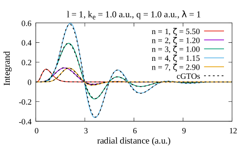
Generally speaking, the evaluation of integrals (6) and (7) can be challenging due to the oscillations in the integrand. Their frequency, amplitude and range depend on the set of parameters and . To illustrate how these parameters act, we plot in Fig. 1 the integrand of (6) for different sets, being kept fixed to 1. Since the analysis of (7) is quite similar, it will not be given here. The values taken for the parameters are dictated by typical applications to lowenergy ionisation processes [7, 11]. In the four panels of the figure, we fix all the parameters except one which is varied and presented in the three sub-panels. In each of the 12 sub-panels we plot the integrand for and its representation with cGTOs (that is to say the sum of the integrands of equation (11)).
The left top panel shows how the exponent acts on the extension of the integrand. A small leads to a larger effective integration range and consequently the effective number of oscillations to be accounted for is increased. The right top panel illustrates that the frequency of the oscillations is increased when the wave number is increased. Note that, in the cGTOs representation (10), for each a different set of linear coefficients is optimized. The left bottom panel shows a similar trend (increase of frequency) but related to increasing values of ; contrary to the previous panel, is fixed and the same GTO expansion is used for the three values. In the right bottom panel we can see that changes mainly the positions of the nodes and the amplitudes of the oscillations. For each , a different set of exponents and linear coefficients of cGTOs are optimized.
The value of - the index of the Bessel functions - also regulates the amplitudes and position of the oscillations (except for ).
The insets in the 12 sub-panels show how the integrand may oscillate up to large distances, albeit with rather small amplitudes. This indicates that the numerical evaluation of the corresponding integrals must be performed with care, since positive and negative contributions appear up to, in principle, infinity.
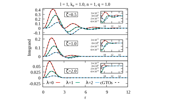
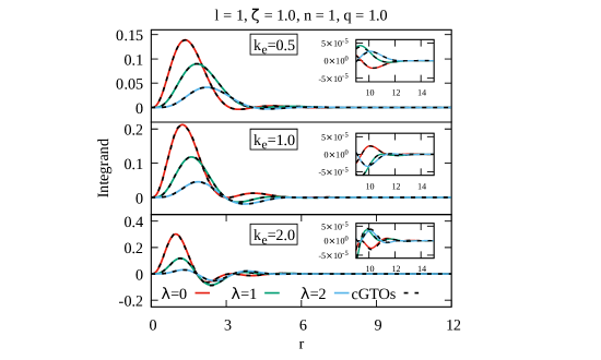
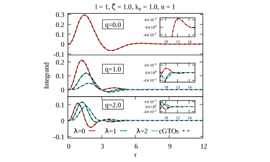
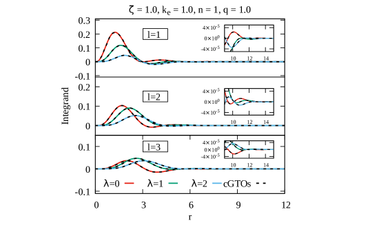
For all the plotted curves, one observes that the cGTOs provide a very good accurate fitting on the whole domain. In physical applications, the range of the integrand of (6) and (7) depends on the electronic extension of the molecule; for small molecules, such as NH3 or CH4, a.u. is generally more than sufficient. To show this, in Fig. 2, the integrand of (6) is plotted with realistic molecular orbitals taken from the literature, for fixed a.u., a.u. and . For the present illustration we have selected, among the molecular orbitals optimized and tabulated by Moccia [16, 17, 18], five sets of corresponding to the most diffused STOs (i.e., the smallest exponent for ). They are the most difficult to represent, and the evaluation of the corresponding radial integrals is the most delicate. Contrary to Fig. 1, here varies; the factor provides at larger distances extra weight to the integrand. In all five cases, the cGTOs representation with reproduces very well the exact integrands.
3.2 Reference value and error related to the range of integration
All integrals (6) or (7) can be evaluated with a numerical quadrature, and the result will be labelled with the superscript “quad”. To do so, we employ the Fortran library QUADPACK [19] where automatic routines are used to perform the integration with relative error tolerance of . Since for the particular case of a regular Coulomb radial function the integral (11) is known analytically, this numerical quadrature could be counterchecked.
As a first stage, we focus on the effective range of the integrals. Figures 1 and 2 showed that the integrand may oscillate up to large distances. Although the bound state finally makes the amplitude tend to zero, the value needed for the upper bound of the quadrature will determine the final accuracy of the integrals evaluation. To investigate the importance of the range of integration, we define the relative error
| (18) |
where corresponds to the distance after which the integrand contribution is smaller than the tolerance error. We also assume that is sufficiently accurate as to be considered as the exact reference.
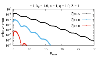
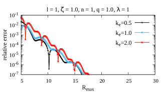
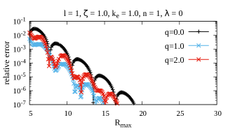
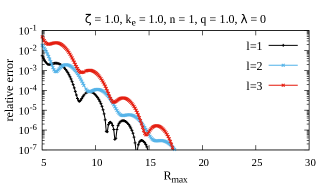
The behaviour of the relative error in terms of the upper bound is shown in Fig. 3. To illustrate the impact of each parameter we present four panels in each of which only one parameter is changed. In all cases as in Figure 1. One can see that, for all cases considered, is sufficient to achieve an acceptable accuracy (lower than ). This tells us that if we want to evaluate the integrals with the analytical approach proposed in subsection 2.3, the cGTOs representation must be reliable up to about (this is the radial domain we have considered here and in previous applications [6, 7, 8]).
3.3 Comparison of integrals: numerical quadrature versus analytical cGTOs approach
We now wish to check the reliability of the cGTOs representation to analytically evaluate the integrals through expression (13) and (17). For a quantitative comparison, we define the relative errors
| (19) | ||||
| (20) |
with respect to the reference values obtained by precise numerical quadrature.
In Tab. 1, we tabulate the values of the reference integrals (6), the cGTOs integrals (13) with , and the relative error (19) for the 36 different sets of parameters considered in Fig. 1. Although it is difficult to establish a strict dependence of these errors on each parameter, we can make the following general observations: by decreasing , the extension of the integrals becomes larger and so does the error; the larger the wave number , the faster the oscillations in , and therefore the larger the error; the variation of and does not lead to any trend. While the change in has a direct impact on the quality of the cGTOs, the change of and does not affect them but influences the oscillating nature of the integrand.
The relative errors vary between and . We notice that amongst the 36 cases the largest errors appear for integrals whose absolute value is rather small. Moreover, while individual integrals may not be perfectly evaluated, one has to take into account that in applications they enter partial wave summations for which rather rapid convergence is usually expected with respect to the and values.
We performed a similar study by comparing the integrals (7) obtained by quadrature and the cGTOs integrals (17) with . Tab. 2 reports the relative errors (20) for four values and five values, while keeping the other parameters fixed to . The relative errors range from to . Quite logically, larger relative errors are observed for smaller values (more diffused bound states) and for larger values (enhanced weight on larger distances though the term ).
Finally we consider again the five sets of parameters associated with the realistic molecular orbitals considered in Fig. 2. In Tab. 3 we tabulate the integrals (6) and the corresponding relative error (19) generated by a cGTOs representation with . We observe that the error remains smaller than , the worse case scenario being for and . Here we should point out that in the tables provided by Moccia that molecular orbital, for example, is accompanied by a relatively rather small coefficient in the expansion (5). Moreover, one has to recall that in physical applications the integrals with small value will have little weight in the overall calculation of matrix elements.
3.4 Convergence with respect to the number of cGTOs
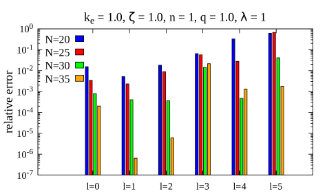
To close the analysis, we investigate the number of cGTOs required for a good representation of the continuum radial functions and the consequence on the integrals evaluation. Fig. 4 shows the relative error (19) with cGTOs for and for fixed parameters . We recall here that, due to the non-linear cGTOs optimization scheme [6], the error corresponding to an energy does not decrease in a monotonic way with . For the chosen parameters, cGTOs turns out to be a reasonable choice to get an acceptable accuracy for angular momenta . On the other hand and cGTOs provide a good representation only for small values of . Going to cGTOs improves slightly the quality.
|
|
|
|
|
|
|
|
|
|
|
|||||||||||||||||||||||||||||||
|
|
|
|
|
|
|
|
|
|
|
|||||||||||||||||||||||||||||||
|
|
|
|
|
|
|
|
|
|
|
|||||||||||||||||||||||||||||||
|
|
|
|
|
|
|
|
|
|
|
|||||||||||||||||||||||||||||||
|
|
|
|
|
||||||||||||||||||||||
|
|
|
|
|
||||||||||||||||||||||
|
|
|
|
|
||||||||||||||||||||||
|
|
|
|
|
|
|
+0.0046639 | +0.0046643 | 0.000079 | +0.001005011 | +0.001005014 | 0.000003 | +0.0001594588 | +0.0001594594 | 0.000004 | |||
|
|
+0.318374 | +0.318202 | 0.000543 | +0.172295 | +0.172431 | 0.000789 | +0.030050 | +0.030309 | 0.008624 | |||
|
|
+0.925984 | +0.926280 | 0.000319 | +0.312400 | +0.312567 | 0.000533 | -0.235702 | -0.235400 | 0.001280 | |||
|
|
+1.512731 | +1.514143 | 0.000933 | +0.310337 | +0.309939 | 0.001283 | -0.686099 | -0.686402 | 0.000442 | |||
|
|
+0.206853 | +0.206441 | 0.001990 | +0.132105 | +0.132482 | 0.002849 | +0.021776 | +0.022351 | 0.026389 | |||
4 Summary
We have presented an investigation of radial integrals involving product of oscillating functions, powers and decreasing exponentials. Two classes are considered corresponding, respectively, to a STO or GTO description of bound states. The oscillating functions are related to an electron in a continuum state that arises, for example, after an atomic or molecular ionization process. The present study illustrated some of the difficulties one may encounter in the evaluation of such integrals. Moreover, using a representation of the continuum radial function in terms of complex GTO, these integrals may be performed analytically and expressed as a sum of special functions. The efficiency and limitation of such an approach are investigated for a range of the integrands’ parameters. In all the tested cases, and even for realistic orbital parameters, the analytical integrals based on approximate cGTO expansions lead to accuracies that are always sufficient for physical applications in the low-energy domain [7, 11].
The present work aimed to grasp the potential of the proposed approach by exploring its reliability for the monocentric case. We consider this step necessary before tackling more difficult integrals, such as two-electron integrals or one electron integrals involving multicentric functions. The ultimate goal would be to reach an all-Gaussian approach to evaluate the necessary integrals involved in scattering processes, similarly to the well known and widely used Gaussian tools and packages used in quantum chemistry.
References
- [1] S. F. Boys, A. C. Egerton, Electronic wave functions - I. a general method of calculation for the stationary states of any molecular system, Proceedings of the Royal Society of London. Series A. Mathematical and Physical Sciences 200 (1063) (1950) 542–554.
- [2] J. G. Hill, Gaussian basis sets for molecular applications, International Journal of Quantum Chemistry 113 (1) (2013) 21–34.
- [3] B. H. Bransden, C. J. Joachain, Physics of atoms and molecules, Pearson Education India, 2003.
- [4] F. P. Prosser, C. H. Blanchard, On the evaluation of two-center integrals, The Journal of Chemical Physics 36 (4) (1962) 1112–1112.
- [5] R. A. Bonham, J. L. Peacher, H. L. Cox, On the calculation of multicenter two-electron repulsion integrals involving slater functions, The Journal of Chemical Physics 40 (10) (1964) 3083–3086.
- [6] A. Ammar, A. Leclerc, L. U. Ancarani, Fitting continuum wavefunctions with complex gaussians: Computation of ionization cross sections, Journal of Computational Chemistry 41 (27) (2020) 2365–2377.
- [7] A. Ammar, L. U. Ancarani, A. Leclerc, A complex gaussian approach to molecular photoionization, Journal of Computational Chemistry 42 (32) (2021) 2294–2305.
- [8] A. Ammar, A. Leclerc, L. U. Ancarani, Multicenter integrals involving complex gaussian-type functions, in: Advances in Quantum Chemistry, Vol. 83, Elsevier, 2021, pp. 287–304.
- [9] W. Magnus, F. Oberhettinger, R. P. Soni, Formulas and theorems for the special functions of mathematical physics, Vol. 52, Springer Science & Business Media, 2013.
- [10] A. R. Edmonds, Angular momentum in quantum mechanics, Princeton university press, 1996.
- [11] A. Ammar, A. Leclerc, L. U. Ancarani, Calculation of electron-impact and photo-ionization cross-sections of methane using analytical gaussian integrals, submitted to Phys. Rev. A (2023).
- [12] H. Bateman, Higher transcendental functions [volumes i-iii], Vol. 1, McGRAW-HILL book company, 1953.
- [13] I. S. Gradshteyn, I. M. Ryzhik, Table of Integrals, Series, and Products, seventh Edition, Elsevier Academic Press, Amsterdam, 2007.
- [14] NIST Digital Library of Mathematical Functions, http://dlmf.nist.gov/, Release 1.1.8 of 2022-12-15, F. W. J. Olver, A. B. Olde Daalhuis, D. W. Lozier, B. I. Schneider, R. F. Boisvert, C. W. Clark, B. R. Miller, B. V. Saunders, H. S. Cohl, and M. A. McClain, eds.
- [15] R. Tomaschitz, Bessel integrals in epsilon expansion: Squared spherical bessel functions averaged with gaussian power-law distributions, Applied Mathematics and Computation 225 (2013) 228–241.
- [16] R. Moccia, One-center basis set SCF MO’s. I. HF, CH4, and SiH4, The Journal of Chemical Physics 40 (8) (1964) 2164–2176.
- [17] R. Moccia, One-center basis set SCF MO’s. II. NH3, NH4+, PH3, PH4+, The Journal of Chemical Physics 40 (8) (1964) 2176–2185.
- [18] R. Moccia, One-center basis set SCF MO’s. III. H2O, H2S, and HCl, The Journal of Chemical Physics 40 (8) (1964) 2186–2192.
- [19] R. Piessens, E. de Doncker-Kapenga, C. W. Überhuber, D. K. Kahaner, Quadpack: a subroutine package for automatic integration, Vol. 1, Springer Science & Business Media, 2012.