Accelerator beam phase space tomography using machine learning to account for variations in beamline components
Abstract
We describe a technique for reconstruction of the four-dimensional transverse phase space of a beam in an accelerator beamline, taking into account the presence of unknown errors on the strengths of magnets used in the data collection. Use of machine learning allows rapid reconstruction of the phase-space distribution while at the same time providing estimates of the magnet errors. The technique is demonstrated using experimental data from CLARA, an accelerator test facility at Daresbury Laboratory.
1 Introduction: machine learning for accelerator beam phase space tomography
Many modern accelerators rely on the production of high-quality particle beams to reach their performance specifications. Facilities such as X-ray free-electron lasers, for example, have demanding requirements for electron beam transverse and longitudinal emittance [1, 2, 3, 4]. Commissioning, tuning and effective operation of many accelerators require the capability to make rapid and reliable measurements of beam parameters at different points along a beamline, often starting at the particle source. In the case of the transverse beam emittance, quadrupole scans provide a standard measurement technique [5, 6]: the emittance is found from the dependence of the beam size (measured using, for example, a wire scanner or imaging screen) on the strength of an upstream quadrupole magnet. The use of tomographic methods [7, 8, 9, 10, 11, 12, 13, 14] allows the transverse phase-space distribution of the beam to be reconstructed from the screen images, yielding not just the emittance but also the optics functions describing how the distribution changes along the beamline. In addition, phase space tomography can provide information on coupling between transverse planes [15, 16] and on the detailed charge distribution within bunches. With the use of RF transverse deflecting structures, it is possible to make detailed measurements of the longitudinal phase space [17, 18]. Combining quadrupole scans with a transverse deflecting cavity makes it possible to determine the five or six-dimensional phase-space beam distribution [19, 20, 21, 22].
Despite the fact that phase space tomography based on quadrupole scans is a well-established technique, there remain several significant challenges in its application, especially for low-emittance beams. Data collection and processing can be time-consuming, especially for higher-dimensional phase space reconstruction. Traditional tomography algorithms can be prone to artefacts in the reconstruction, especially when the range or number of projection angles is limited (as is often the case in beam phase space tomography) [23, 24]: although there are techniques that can be used to reduce the appearance of reconstruction artefacts (see, for example, [25]), ultimately the fidelity of the reconstruction depends on collecting screen images with a sufficient number of different strengths of the upstream quadrupoles, setting a lower limit on the time needed for data collection and analysis. Machine learning (ML) techniques have been shown to be of value for tomography [26], including for phase space tomography in particle accelerators [27, 28], but the use of ML for this purpose is relatively new and there is significant scope for improvement in the methods and tools available.
Reconstruction of the beam phase-space distribution in an accelerator using quadrupole scan data is further complicated by the possible presence of errors in accelerator components. For example, errors in magnet strengths, screen calibration errors, beam energy errors or the presence of dispersion (e.g. from magnet alignment errors) can all have a significant impact on the results. Errors in the field strength in a magnet may arise from hysteresis, calibration errors in magnet manufacture, power supply or control system errors, or short-circuits within the coils of the magnet. The beam energy may vary during a measurement as a result of fluctuations in RF power amplitude or phase in linacs or an RF gun. Although significant efforts are generally made to minimise errors in accelerator systems, even a relatively small accelerator facility can contain hundreds or thousands of components, and access to an accelerator by technical personnel to confirm that components are working correctly will involve interrupting machine operation during the inspection. As a result, even quite large errors can sometimes be present in components used in quadrupole scan measurements, and beam diagnostics techniques that allow for (and provide information on) various errors in accelerator components would be of significant value in accelerator tuning and operation.
One approach to accounting for variations in accelerator conditions (including component errors) in diagnostics measurements is to use a neural network that can be tuned to adapt to changes in the relevant accelerator systems. ‘Tunable’ neural networks have been used in high-energy physics [29] and in the reconstruction of phase-space distributions in accelerators [30]. Scheinker et al. [31, 32, 33] have proposed the use of a low-dimensional latent space in an encoder-decoder architecture: by tuning the latent space so that the decoder output matches the observations, the ‘true’ encoding of the quantity or property to be measured can be obtained. For example, the input to the encoder may be a set of projections from a beam distribution in phase space onto a co-ordinate axis, with the output from the decoder being the full phase space distribution. Given the phase space distribution, the projection onto a co-ordinate axis is readily found, and the latent space is adjusted (from a starting point determined by the input to the encoder) so that the computed projection matches as closely as possible the observed projection. A similar approach has been used by Roussel et al. [30, 34] in the reconstruction of the four-dimensional phase-space distribution in a wakefield accelerator.
In the work presented in the current paper, we adapt the latent space tuning technique to identify quadrupole strength errors in beam phase space tomography measurements. Our approach differs from previous work in that rather than tuning the neural network (or latent space) so that the output matches as closely as possible the observations, we train a network using data from a simulation that includes known errors. This avoids the need for an optimization routine for tuning the neural network, and potentially allows information on the accelerator conditions to be obtained directly in addition to the primary intended measurement. Although the technique is generally applicable to a wide range of different diagnostics on various types of accelerator, in this paper we illustrate its use for reconstructing the charge distribution in phase space in CLARA, an accelerator test facility at Daresbury Laboratory [35, 36]. Phase space measurements in CLARA using ML have been reported in an earlier paper [27]: in the present work, we show the results of a new analysis of some of the previous data using the new method, based on neural networks trained on data from simulations including machine errors. At the core of the technique is the use of an autoencoder (trained on simulated screen images in the absence of magnet errors) to construct a latent space that encodes both the observed screen images and the phase space distribution. The latent space is extended by appending the magnet errors: the beam distribution in phase space upstream of the magnets is still described by just the original latent space; but by appending the quadrupole errors we construct an ‘extended latent space’ that encodes the screen images in the presence of the quadrupole errors. A second neural network is then trained to take the observed screen images in the presence of magnet errors as input, providing the extended latent space as output. By this means, given a set of screen images from simulations or measurements in the presence of magnet errors, both the phase space distribution and the magnet errors can be found.
Results from phase space tomography can generally be validated by reconstructing observed screen images from simulations using the phase space distribution obtained from tomographic analysis. We find that with the method described in this paper, individual screen images are not reproduced with the same level of detail as in the previous reported analysis of data from CLARA: this is to be expected, since representing the screen images (or, equivalently, the phase space distribution) using a relatively small set of components in a latent space inevitably entails some loss of information. But importantly, we find that the new approach leads to a phase space distribution that better fits the overall observed variation in beam size over the course of the quadrupole scan. The results of the extended latent space technique also indicate significant errors in the quadrupole strengths, which may partly be explained by an error in the beam energy.
We should emphasise that the goal of the technique presented here is not to achieve a highly-detailed reconstruction, providing accurate information on fine structures in the phase space distribution. In many situations (e.g. when commissioning or tuning an accelerator) it is more important to be able to predict accurately the overall variation in beam size as the beam propagates along a beam line, and how the beam size responds to changes in quadrupole strengths. Especially in the early stages of accelerator commissioning or after restarting from a shut-down period, it is also important to be able to identify possible errors in accelerator components. The aim of the current work is to demonstrate a technique that has the potential to meet these needs. Development of the technique was partly motivated by the later analysis of the data reported in [27] that suggested significant errors on the magnets, or on the beam energy (or both). In particular, it was found that if it was assumed that there were some errors on the magnets used in the quadrupole scan, then the phase space distribution obtained from the tomography analysis led to a better fit to the observed variations in beam size over the course of the scan. However, with the usual tomography algorithms it is difficult to perform a fully self-consistent analysis in a systematic way, and to determine possible errors with any confidence. This is because tomographic analysis depends on the assumed strengths of the magnets used for the scan, and computing the phase space distribution with errors on the magnets involves repeating the full analysis for each set of magnet errors. For tomography in two (or more) degrees of freedom, the time required makes it impractical to use optimisation routines to fit errors on the quadrupoles. Even if a neural network was used for the phase space reconstruction, different sets of training data would be needed for different magnet errors. Using existing techniques, fitting both the phase space distribution and the magnet errors in a systematic and fully consistent way would be an extremely time-consuming process. In practical situations, the time taken for data processing and analysis is a significant consideration, and given the possibility of (perhaps significant) errors on the components used in a diagnostics measurement, the extended latent space technique that we describe in this paper could be of value in tuning and operating an accelerator.
The paper is organised as follows. In section 2 we describe the principles on which the ML technique described in the current work is based. There are a number of possible variations on the structure of the neural networks, and the way in which the latent space is constructed: in section 3 we describe one option in more detail, including examples of the training data and results from the neural networks using simulated test data. As an illustration of the application of the technique to experimental data, in section 4 we present results from CLARA. Finally, in section 5 we discuss the potential benefits and possible limitations of the technique, and outline potential areas for further development.
2 Tomography with extended latent space to account for errors on accelerator components
Phase space tomography aims to construct the distribution of particles in phase space at a chosen point in an accelerator beamline (the ‘reconstruction point’) from images collected on a diagnostics screen as a downstream location (the ‘observation point’). Between the reconstruction point and the observation point, a number of quadrupoles are used to control the evolution of the beam distribution. By choosing appropriate strengths for the quadrupoles, it is possible to rotate the distribution in phase space, changing the projection of the phase space distribution onto co-ordinate space: a rotation through 90∘ (for example) interchanges co-ordinate and momentum variables. Thus, observing the co-ordinate distribution provided by the screen image for a range of rotation angles (corresponding to different quadrupole strengths) allows reconstruction of the distribution as a function of both co-ordinate and momentum.
As well as determining the rotation in phase space between the reconstruction point and the observation point, the quadrupoles between these two points will determine the horizontal and vertical beta functions that characterise the size and shape of the image observed on a diagnostics screen. Generally, it is desirable to maintain an aspect ratio close to 1 on the screen (i.e. a roughly circular beam image), and to avoid beam sizes that are either very small (approaching the resolution limit of the imaging system) or very large (and as a result, very diffuse and with low average intensity). The quadrupole strengths used in a scan for phase space tomography are therefore determined by the need to cover a good range of rotation angles in phase space while maintaining a reasonable size and shape for the image on the diagnostic screen. For the work reported in this paper (including experimental results from CLARA) the beta functions at the observation point and the phase advances between the reconstruction point and the observation point are shown in figure 1. Although there is some variation in the beta functions over the course of the quadrupole scan, and the horizontal and vertical beta functions are not exactly equal, there is not an absolute requirement for equal, fixed beta functions, and if the beta functions at the reconstruction point correctly describe the phase space distribution, then we expect only small changes in the size and shape of the beam image at the observation point. In practice, we observe much larger changes in size and shape than expected (see, for example, the experimental results shown later, in figure 14): this indicates that the phase space distribution differs from the design specifications. One of the main purposes of the tomography measurement is to determine the real distribution.
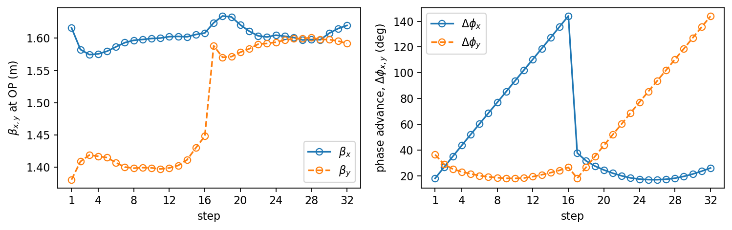
A further consideration concerns the sizes of the data structures used for the sinograms (the set of images collected in a quadrupole scan) and the phase space distribution. This is a particular issue for higher-dimensional reconstruction of the phase space distribution. The screen images could easily have a resolution of order 100100 pixels. If the four-dimensional phase space is reconstructed to the same resolution, the required data structure is a four-dimensional array with a total of components. While the processing of data sets of this size (roughly 1 Gb using double-precision arithmetic) is, in principle, within the capability of modern computers, conventional tomography algorithms will generally require a memory capacity several orders of magnitude larger than the capacity needed just to store the result. Even if machine learning is used, training a neural network with data sets of this size places significant demands on computational power. Image compression techniques can be used to reduce the sizes of the data sets significantly; but it is not clear how conventional tomography algorithms can be used with images in compressed form. However, it was shown in [27] that ML tools can be used for tomography with sinograms (sets of screen images) and phase space distributions in compressed form: the only requirement is that the same information is contained in the compressed image as in the original image. Once the final result (the phase space distribution) is obtained, then the data can be decompressed for visualisation and further analysis. Data compression can conveniently be achieved using discrete cosine transforms (DCTs) [37, 38, 39]: using DCTs it is possible to reduce the resolution by a factor (typically) between five and ten, while retaining much of the information in the original image. This means that the memory required to store a four-dimensional phase space distribution can be reduced by a factor . For the work presented in this paper, we use a DCT resolution of 16: it is found that for the experimental measurements on CLARA, this preserves a reasonable level of detail in the screen images and the phase space distribution [27]. In addition to compressing the images, we work in normalised phase space: this simply involves scaling each screen image horizontally and vertically by and respectively, where and are the nominal horizontal and vertical beta functions at the observation point, for the corresponding step in the quadrupole scan (as shown in figure 1). This simplifies the analysis, and can lead to improved accuracy in the reconstructed phase space [24].
The technique we describe in this paper, for phase space tomography taking into account errors on accelerator components, involves three related neural networks. The relationships between the networks are illustrated schematically in figure 2(a). There are many possible variations on the technique: one example is shown in figure 2(b); however, for simplicity, we focus on the first option, with a latent space obtained using a sinogram autoencoder. In this case, the technique is applied as follows. The first neural network is a ‘sinogram autoencoder’: this takes a set of (DCT compressed) screen images as input, and is trained to give the same screen images as output. Between the input and output layers are a number of hidden layers. The central hidden layer consists of a relatively small number (some tens) of nodes: this is the latent space, which encodes the main features of the sinograms from the training data. For the autoencoder, the training data are constructed from a simulation of the quadrupole scan in an accelerator tracking code, assuming that there are no errors on any of the accelerator components.
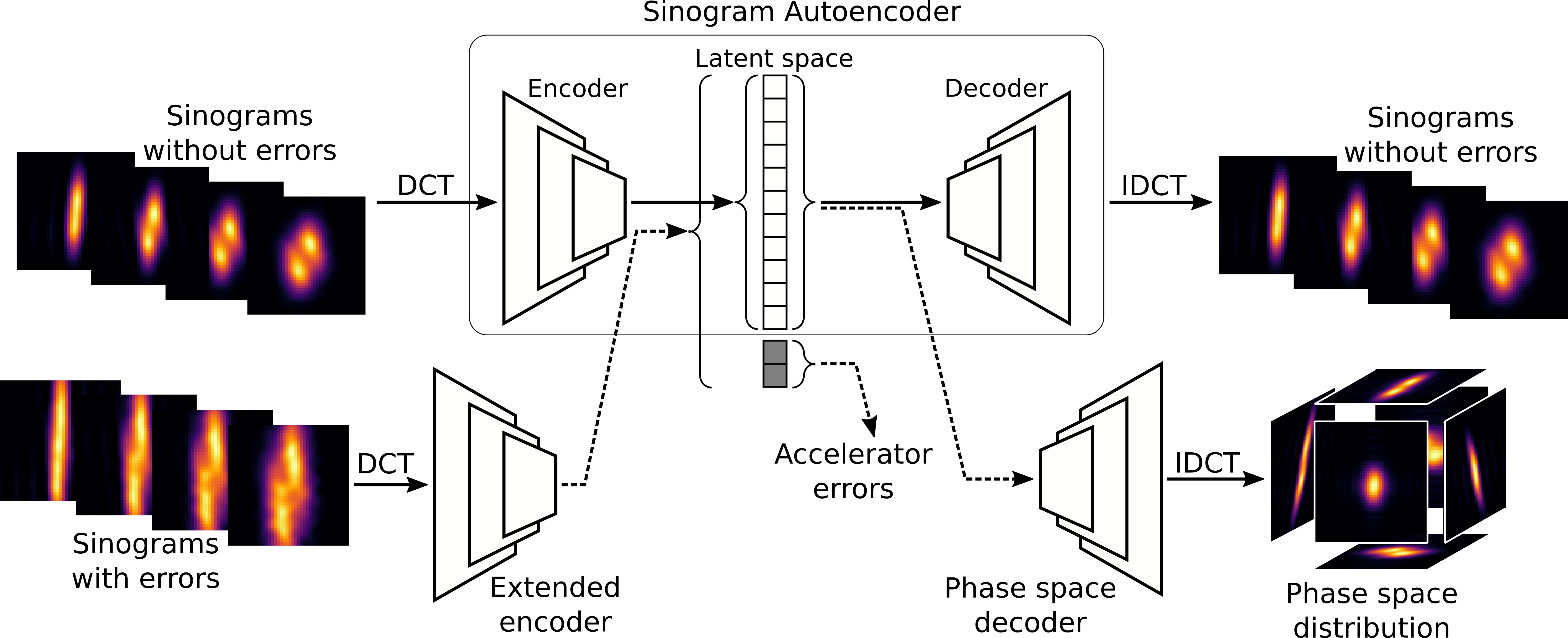
(a) Latent space constructed using a sinogram autoencoder.
(b) Latent space constructed using a phase space autoencoder.
The next step is to construct a second neural network, which we refer to as the ‘extended encoder’. This takes a sinogram as input, and is trained to provide the extended latent space as output. The training data in this case consists of sinograms produced in the same way as for the training data for the sinogram autoencoder and with the same initial phase space distributions, but now with random errors on the quadrupole strengths. The extended latent space is constructed from the latent space from the autoencoder, with additional values (nodes) corresponding to the quadrupole strength errors.
Finally, we construct a third neural network, a ‘phase space decoder’. This takes the (unextended, or ‘basic’) latent space as input, and provides the (DCT compressed) four-dimensional transverse phase space distribution as output.
Once the three neural networks have been trained, a sinogram compiled from images recorded in a quadrupole scan on the accelerator can be provided as input to the extended encoder. The output consists of the latent space encoding the sinogram that would be observed in the absence of accelerator component errors (i.e. the basic latent space), together with a set of values representing the errors present on the components used in the quadrupole scan. The phase space distribution is obtained from the phase space decoder, providing the basic latent space as input. The results may be validated by simulating the quadrupole scan in a tracking simulation, using the phase space distribution obtained from the phase space decoder as the starting distribution, but now including the errors on the accelerator components obtained from the extended latent space. The accuracy of the reconstruction of the phase space distribution may be assessed from the level of agreement between the simulated screen images and the observed images.
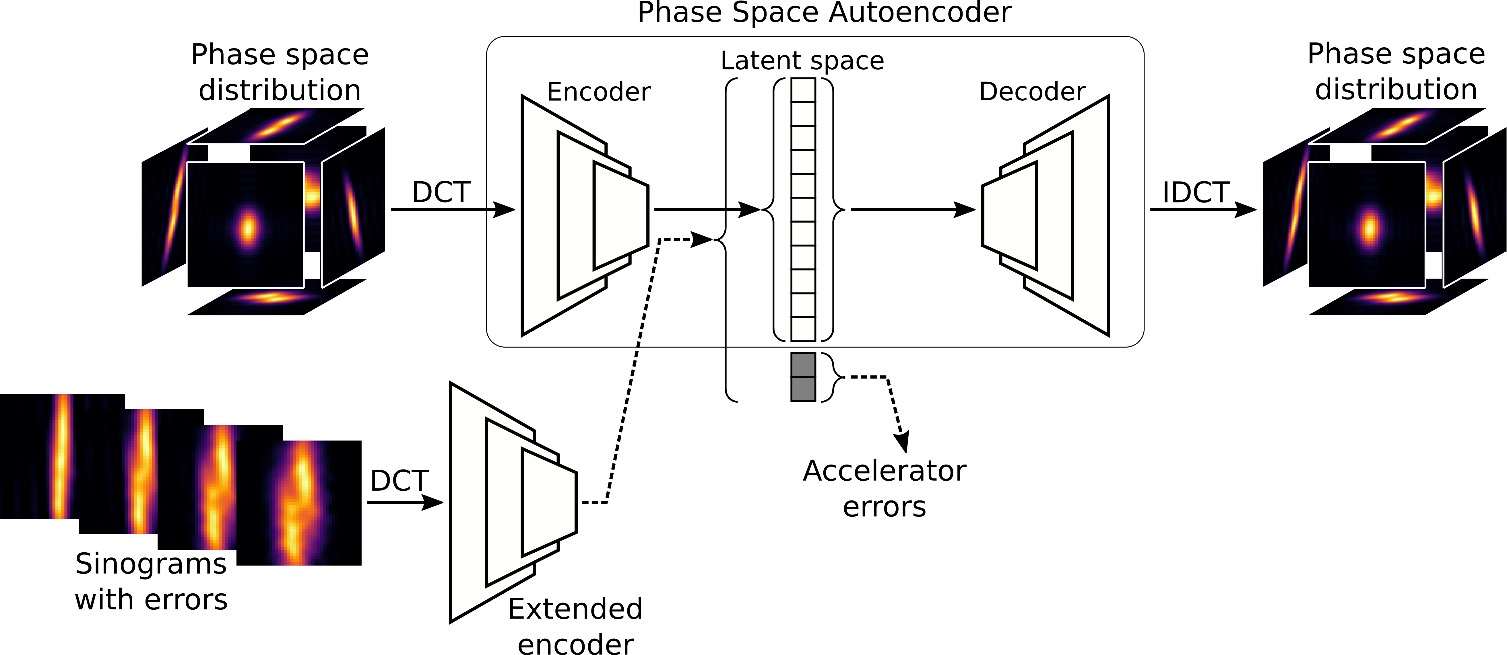
The important feature in this procedure is the use of an extended latent space, constructed from two distinct sets of parameters. The first set of parameters encodes not only the images that would be observed in a quadrupole scan in the absence of errors on accelerator components, but also the beam distribution in phase space. The second set of parameters in the extended latent space encodes the errors on the accelerator components that were present during the collection of beam images during a quadrupole scan. The basic principle of an extended latent space can be implemented in various ways, with different relationships between the neural networks. The particular method just described, and discussed in further detail in the following sections, is illustrated in figure 2(a); another possible implementation is shown in figure 2(b). In the latter case, the basic latent space is constructed from an autoencoder for the phase space distribution. This avoids the need for a separate phase space decoder; however, we have found that an autoencoder for the sinograms performs better for test data than an autoencoder for the phase space distributions. This may be because of differences in the sizes of the data sets, which has a direct impact on the numbers of nodes needed in the layers of the neural network.
In a further variation, the basic latent space could be constructed not from an autoencoder, but from principal component analysis of the sinograms (without errors on the accelerator components) or of the phase space distributions: autoencoders were originally proposed as an alternative to principal component analysis for dimensionality reduction [40]. We have found that constructing the latent space using an autoencoder usually leads to a reconstruction of test data that is more accurate than if principle component analysis is used, though the difference is not very great. For phase space tomography on CLARA, the procedure represented in figure 2(a) appears to work somewhat better than alternatives we have tried, but it is possible that in other cases (for example, with differences in the design of the experiment, or for different machine conditions) an alternative technique may produce better results.
Application of the extended latent space technique in a real machine relies on the validity of a number of assumptions. One important assumption is that the basic latent space provides an accurate description of both the sinograms (without errors on accelerator components) and the corresponding phase space distributions. This requires the quadrupole scan to cover a wide range of phase space rotation angles (ideally, 180∘ in each degree of freedom), with a sufficient number of steps. If the range of angles is too small or if there are two few steps, then the phase space distribution will not be fully characterised by the sinogram, and the problem of finding a distribution that reproduces a given sinogram will be underconstrained.
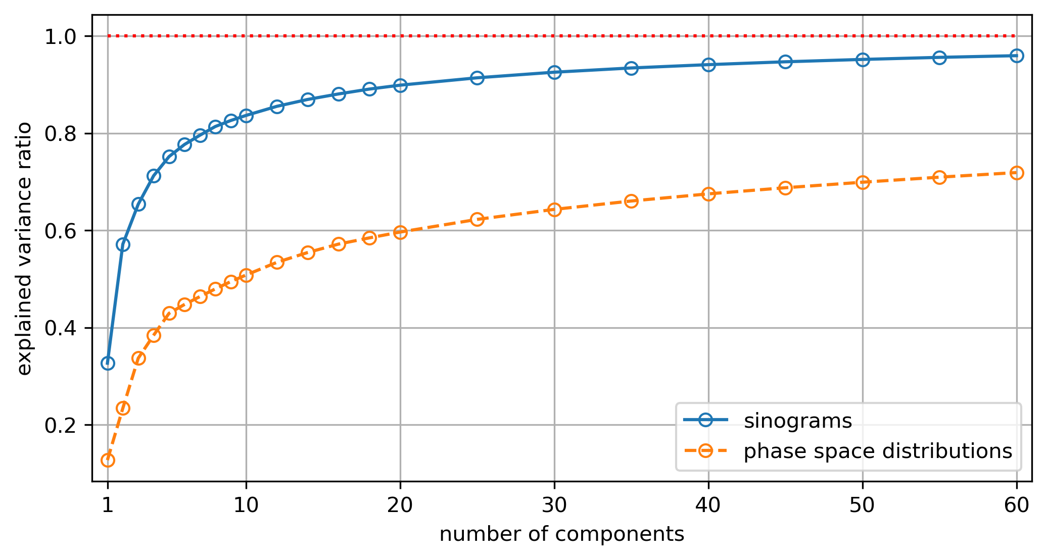
An indication of the extent to which the phase space distribution is determined by a sinogram can be obtained from principal component analysis (PCA). In particular, we calculate the explained variance ratio for different numbers of PCA components for the sinograms and the phase space distributions: the results for the case considered in this paper (with 32 steps in a quadrupole scan) are shown in figure 3. Using (for example) 40 PCA components, the explained variance ratio for the sinograms is 0.94, compared to 0.68 for the phase space distributions. This means that using a latent space with 40 components, we would expect to be able to describe the sinograms with significantly greater accuracy than the phase space distributions. To improve the accuracy of description of the phase space distributions, we would need to increase the size of the latent space. However, the explained variance ratio increases rather slowly when the number of PCA components is increased above 40, and making the latent space too large is not desirable since this would reduce the relative weight of the (small number of) errors on the accelerator components when these are included by extending the latent space. Alternatively, improving the accuracy of reconstruction of the phase space distribution might be achieved by some modification of the quadrupole scan, for example increasing the number of steps or optimising the steps used. However, increasing the number of steps in a quadrupole scan would increase the time needed for data collection on the accelerator. For the current work, we accept the limitations on the accuracy of the reconstruction of the phase space suggested by the explained variance ratios.
The extended latent space technique for phase space tomography also assumes that the accelerator component errors included in the extended latent space correspond to the errors affecting the screen images observed in the accelerator. When the training data for a neural network are produced using a computer model of an accelerator, the physical effects represented in the model are implicit in the training data. This does not, of course, guarantee that results from the neural network will always respect the physics in the model, although if the network is designed and trained properly then the neural network results should be close to the simulation results. But the fact that the training data are constructed from simulations does mean that the neural network cannot be expected to model physical behaviour not present in the computational model of the accelerator. As an example, consider the case that there is dispersion present in the section of beamline used in the quadrupole scan when collecting data, but which is omitted from the model. In the real accelerator, varying the quadrupole strengths will vary the dispersion at the observation point, and because of the energy spread on the beam, the variation in beam size in the accelerator during the quadrupole scan will differ from the variation expected from the computational model. This will be the case even if all other aspects of the system are represented accurately. As a result, if the model is used to reconstruct the phase space distribution from observed screen images, the distribution that is obtained will not exactly match the distribution in the accelerator. Furthermore, using the reconstructed phase space distribution in a simulation of the quadrupole scan will produce screen images that differ from those observed experimentally. The reconstructed phase space distribution can always be validated by using the distribution in a simulation of the quadrupole scan, but differences between the observed and simulated images may arise either from limitations on the technique (for example, if the reconstruction of the phase space distribution is not properly constrained by the sinogram) or from differences between the physics in the real accelerator and the physics included in the computational model.
3 Implementation of the extended latent space technique: an example
3.1 Training data
Phase space distributions
The training data used for the neural networks should resemble the phase space distribution that we expect to see in the accelerator, while including sufficient variation to allow for some significant differences from the expected distribution. Ideally, the transverse phase space distribution in CLARA would be described by a four-dimensional Gaussian function. In practice, we observe some detailed structure in the screen images [27]: the precise features depend on the machine conditions and can also change over time. The difficulty in knowing in advance what kinds of detailed structure may be observed presents some challenges in generating appropriate training data. To allow for a suitable range of possible distributions in phase space, we base the training data on Hermite–Gaussian modes. In normalised phase space with co-ordinates , we first construct a Hermite mode :
| (3.1) |
where is a vector with components , is the Hermite polynomial of order , is a vector in normalised phase space, and is a constant associated with the width of the distribution. The density of particles in phase space is obtained by summing over modes with random amplitudes , and with random four-dimensional rotations , ‘stretch’ transformations and translations applied to each mode:
| (3.2) |
Here, is chosen so that the peak density is . For the training data used in the examples presented here, we use four modes for each case. Some examples of phase space distributions from the training data constructed in this way are shown in figure 4.
Case A
Case B
Case C
Sinograms
To construct the sinogram corresponding to a given phase space distribution, a set of particles is created in the computer simulation with the given distribution in phase space, and the co-ordinates of the particles are transformed from the normalised phase space to the accelerator phase space in the usual way:
| (3.3) |
Here, , , and are the Courant–Snyder parameters at the reconstruction point. After tracking particles from the reconstruction point to the observation point, the co-ordinates of particles are transformed back to normalised phase space, using the inverse of the transformation in equation (3.3), with the appropriate values for the Courant–Snyder parameters at the observation point. A simulated screen image is obtained by projecting the particle distribution onto the – plane.
Quadrupole errors
For each phase space distribution, sinograms with and without errors on the quadrupole magnets are constructed. Errors on the quadrupoles are applied randomly, but are systematic in the sense that a given magnet has a constant scaling factor applied to its strength at each step in the quadrupole scan. Thus, for a given case in the training data, the strength of a magnet in the presence of errors is given by:
| (3.4) |
where is the nominal quadrupole focusing strength, is the focusing strength in the presence of an error, and is a random number from a flat distribution within a chosen range. For the case of CLARA, we choose a range , i.e. errors on the magnet strengths are in the range . Although the magnet strengths in the accelerator are expected to be within a much smaller range (in principle, less than ) of their nominal values, a much larger range is used for the training data partly to explore whether the the technique works with large errors, but mainly to allow for the possibility of very large errors actually occuring in practice. Although a different error is applied to each of the five quadrupoles in the scan, a non-zero mean error over the five magnets could correspond to an error in the beam energy: the effect of an increase in strength of all five magnets by 10% would be similar to the effect of a reduction in beam energy by 10%. During experimental data collection, nominal system settings were used for an intended beam energy of ; however, because of time constraints the actual beam energy was not confirmed by direct measurement.
Errors on the quadrupole magnets can have a significant impact on the screen images at the observation point: this is illustrated (for simulated data) in figure 5. Note that the effect on the beam images depends not just on the average error over all quadrupoles, but also on how the errors vary from one quadrupole to the next. For example, if two adjacent magnets have similar errors, then the effect of the errors will depend on whether the magnets have the same polarity (in which case the effects of the errors will combine) or opposite polarity (in which case there may be some cancellation).
We note that the model used here for errors on the quadrupole magnets is a greatly simplified representation of the errors that may occur in practice. For example, the error on a given magnet may vary with magnet strength because of hysteresis effects: this may particularly be the case when the polarity of a magnet changes sign. Nonlinear or time-dependent effects in the magnet power supplies may also lead to complex behaviour of the magnet errors. To try to reduce hysteresis effects, the order of steps in the quadrupole scan was designed to minimise the number of times that any magnet would need to change polarity. However, changes in polarity could not be avoided altogther and about half-way through the scan, a change in polarity was needed for several of the magnets: at this point, when collecting data experimentally, the magnet strengths were cycled to return the cores of the magnets to a nominal operating point on the magnetisation curve. The magnets were also cycled immediately before a quadrupole scan was performed.
The computational model of the accelerator was used to construct training data consisting of 20,000 phase space distributions together with the corresponding sinograms. A subset of 18,000 cases was used in training the neural networks (the ‘training set’), and the remaining 2,000 cases were reserved for testing the trained networks on unseen data (the ‘test set’). The data were scaled so that each sinogram (consisting of a set of 32 images) had DCT values in the range -1 to +1, with the values representing the magnet errors lying in the same range.
3.2 Sinogram autoencoder
We use Keras [41] for all the machine learning tasks described in the current work. The first neural network to be constructed is the sinogram autoencoder. The input and output data consist of the discrete cosine transform (DCT) of each simulated screen image, without quadrupole errors. The input and output layers are flat layers consisting of 8,192 nodes, corresponding to 32 images with DCT truncation to 16 components in each transverse dimension. We use five hidden layers (with 1,600, 400, 40, 400 and 1,600 nodes): the latent space is given by the central layer, and so has dimension 40. An example of results from the autoencoder with test data is shown in figure 6.
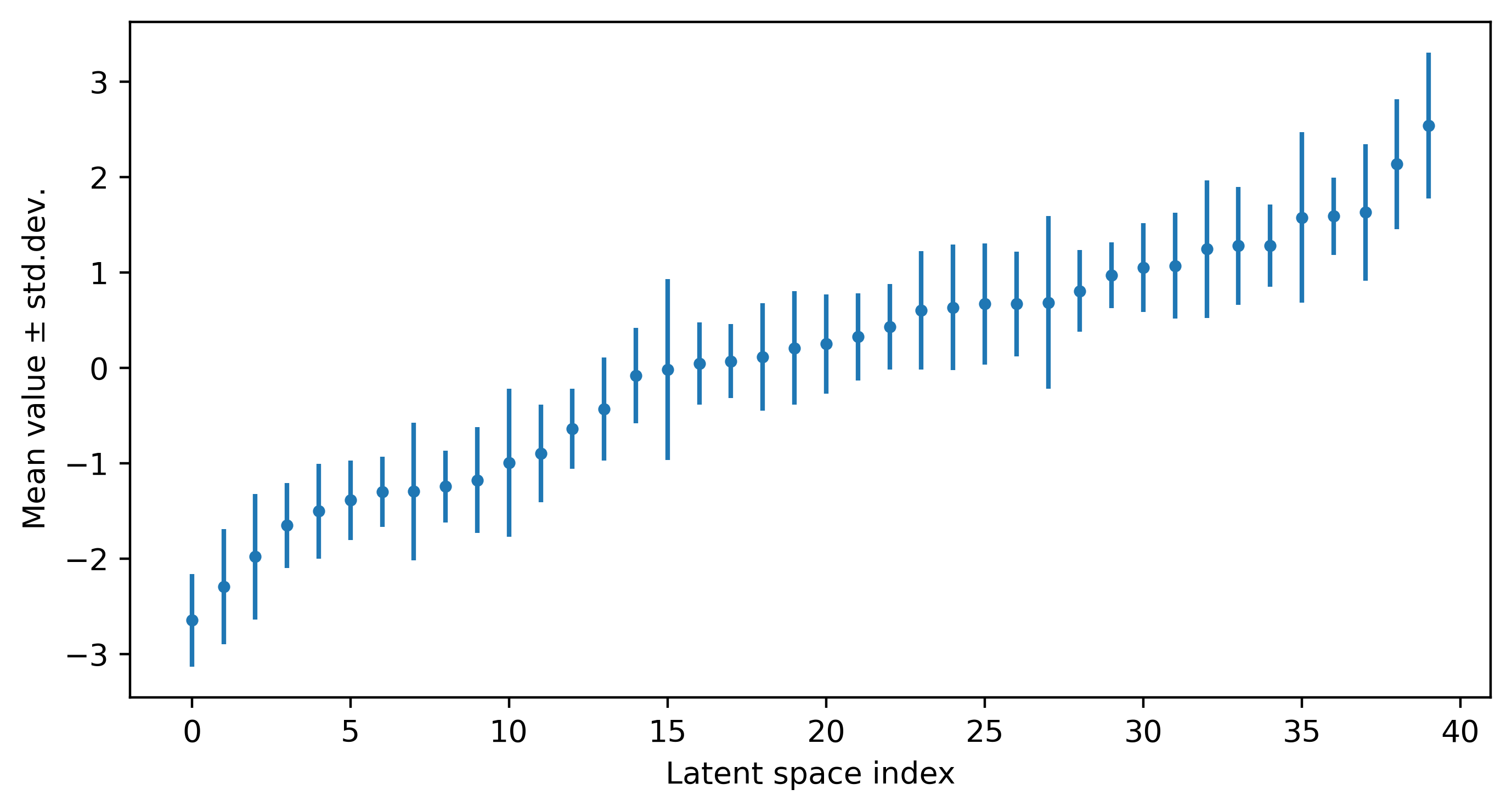
Using a latent space with 40 components, it is possible to describe even quite detailed features in the sinograms with good accuracy: this is consistent with the PCA results, which suggest an explained variance ratio of 94% with 40 PCA components. The latent space values obtained from the training data are shown in figure 7. Note that for this plot, the latent space components have been sorted in ascending order of the mean value across all cases in the training data. The vertical bars show the standard deviation of each component.
3.3 Extended encoder
The next step is to construct an extended encoder to predict the extended latent space (i.e. including errors on the quadrupole magnets) from a given sinogram. The structure for the extended encoder is similar to that of the first half of the sinogram autoencoder, and consists of a flat input layer with 8,192 nodes, a single hidden layer, and an output layer. The output layer matches the extended latent space: for the examples shown here, it consists of 40 nodes from the latent space of the sinogram autoencoder, plus three nodes for the quadrupole errors. Note that although five quadrupole magnets are used in the quadrupole scan, and errors are applied to all five magnets when constructing the training data in simulation, the errors on the final two quadrupoles (which are close to the observation point) have little impact on the images on the diagnostics screen. As a result, although it is possible to construct a neural network that can predict the errors on all five magnets to good accuracy for the training data, the accuracy of prediction for test data is generally very low. We therefore exclude these two magnets from the extended latent space, and just use an extended latent space of 43 nodes.
For training the extended encoder, we double the size of the training data set by combining the data sets with and without quadrupole errors: the sinograms without errors can be considered a special case of the sinograms with errors, in which the errors are zero.
For the extended encoder, we find that overfitting can be a problem: training the network can result in a network that ‘predicts’ the extended latent space with very high accuracy for the data used in training, but with relatively poor accuracy for the test data. Reducing the size of the network helps to some extent: this is the reason for using just a single hidden layer in the extended encoder. Other strategies for avoiding overfitting (such as the use of dropout layers) appear to have little benefit; however, applying L2 regularisation [42, 43] to the hidden layer appears to be effective, and is used for the results presented here.
Correlations between the latent space values obtained from the sinogram encoder and the values predicted by the extended encoder are shown in figure 8 for the first five components of the latent space. For all components, we find a good correlation: for any given component of the latent space, the residuals are small compared to the range of values (across all the training data) for that component. The residuals for the training set and the test set from the training data show similar distributions.
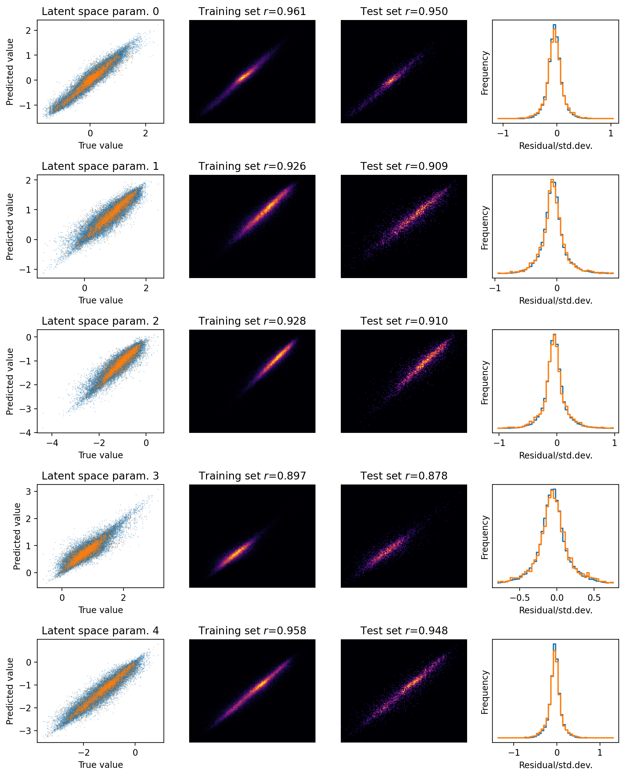
Figure 9 shows the correlations between the magnet errors and the values for the errors predicted by the extended encoder. Although there is still a close correlation between the true values and the predicted values, the residuals are larger than for the components of the extended latent space describing the sinograms. Uncertainties on values for fitted magnet errors may be estimated from the standard deviations of the residuals between ground truth values and predicted values. For the test data, with scaled magnet errors in the range 1, the residuals have standard deviations 0.225, 0.183 and 0.175 for magnets 0, 1 and 2 respectively. Since the errors are in the range 15%, the absolute uncertainties on values for the magnet errors obtained from the extended encoder are 3.4%, 2.8% and 2.6% for magnets 0, 1 and 2 respectively.

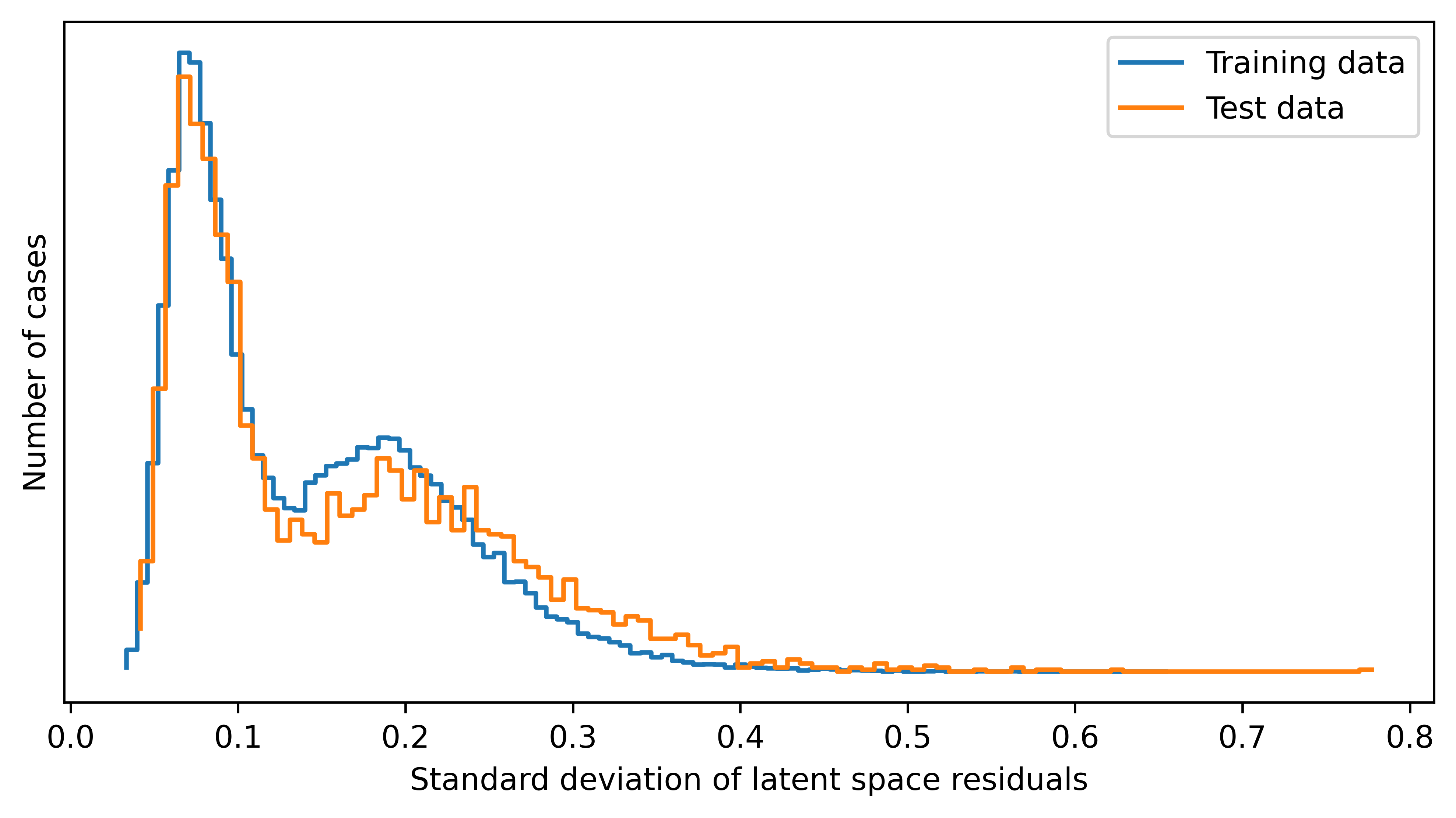
It is worth noting that the residuals for the predictions from the extended encoder are larger for cases with magnet errors than for cases without magnet errors. This can be seen in figure 10, which shows the distribution of the standard deviation (taken over the 43 components of the extended latent space) of the residuals of the extended encoder predictions. The training set and test set are again shown separately, so that it can be seen that the distributions for the two sets are similar: the fact that the residuals for the test data tend to be a little larger than the residuals for the training data suggests that there may be some overfitting, but any overfitting appears to be limited. Both distributions show two distinct peaks, one below a standard deviation residual 0.1, and another (broader) peak around 0.2. Closer inspection of the data shows that the sharp peak below 0.1 corresponds to the cases in training data with zero quadrupole errors, while the broader peak at a higher residual value corresponds to the training data with non-zero quadrupole errors.
3.4 Phase space decoder
The final step is to construct the phase space decoder, a neural network that takes as input the components of the extended latent space describing the sinograms (without quadrupole errors), and provides as output the four-dimensional transverse phase space distribution. The input layer has 40 nodes, corresponding to the latent space of the sinogram autoencoder; the output layer has nodes, corresponding to a DCT resolution of 16 in each dimension of the four-dimensional transverse phase space. Between the input and output layers, there are three hidden layers (with 800, 1,200 and 2,400 nodes).
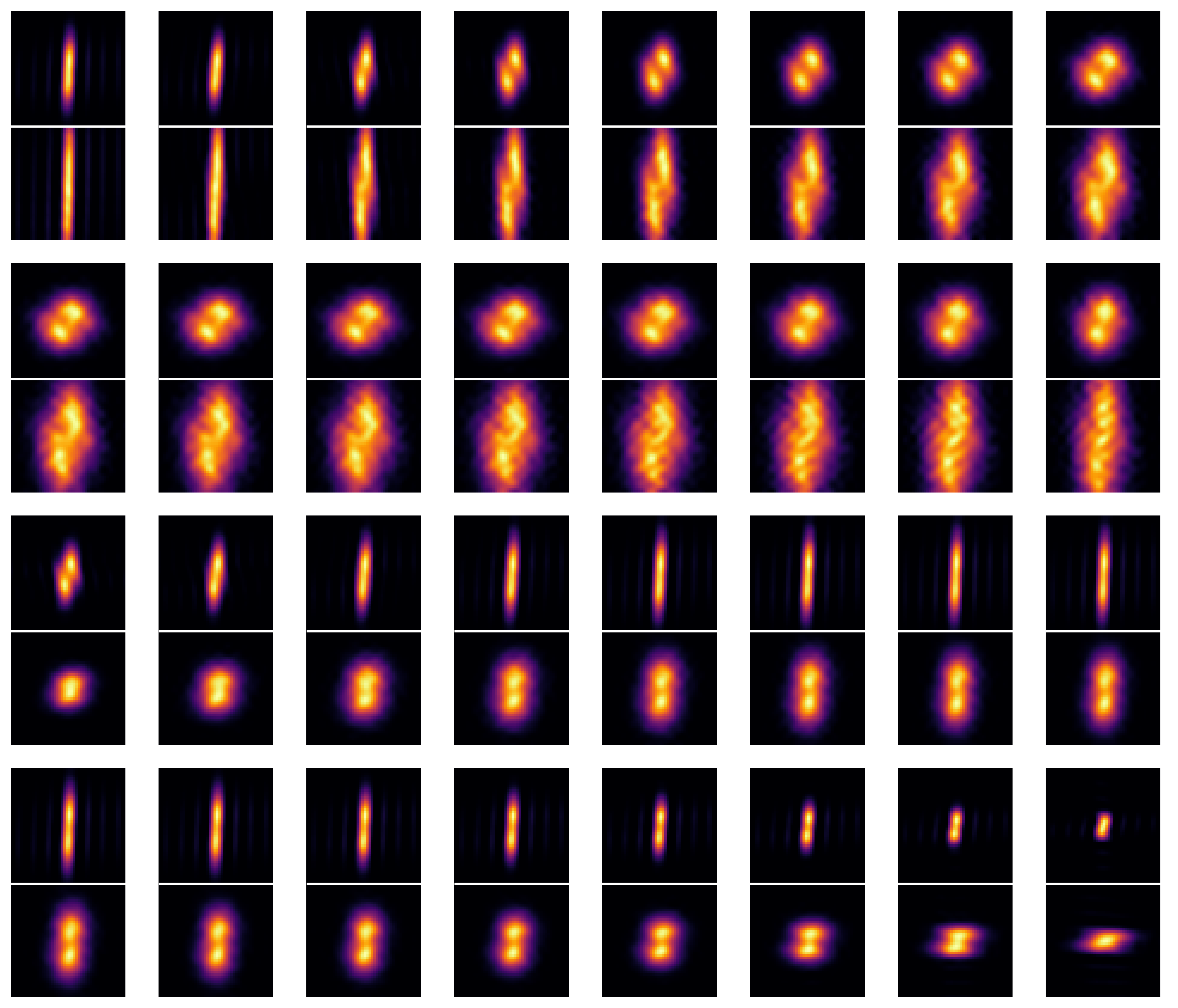
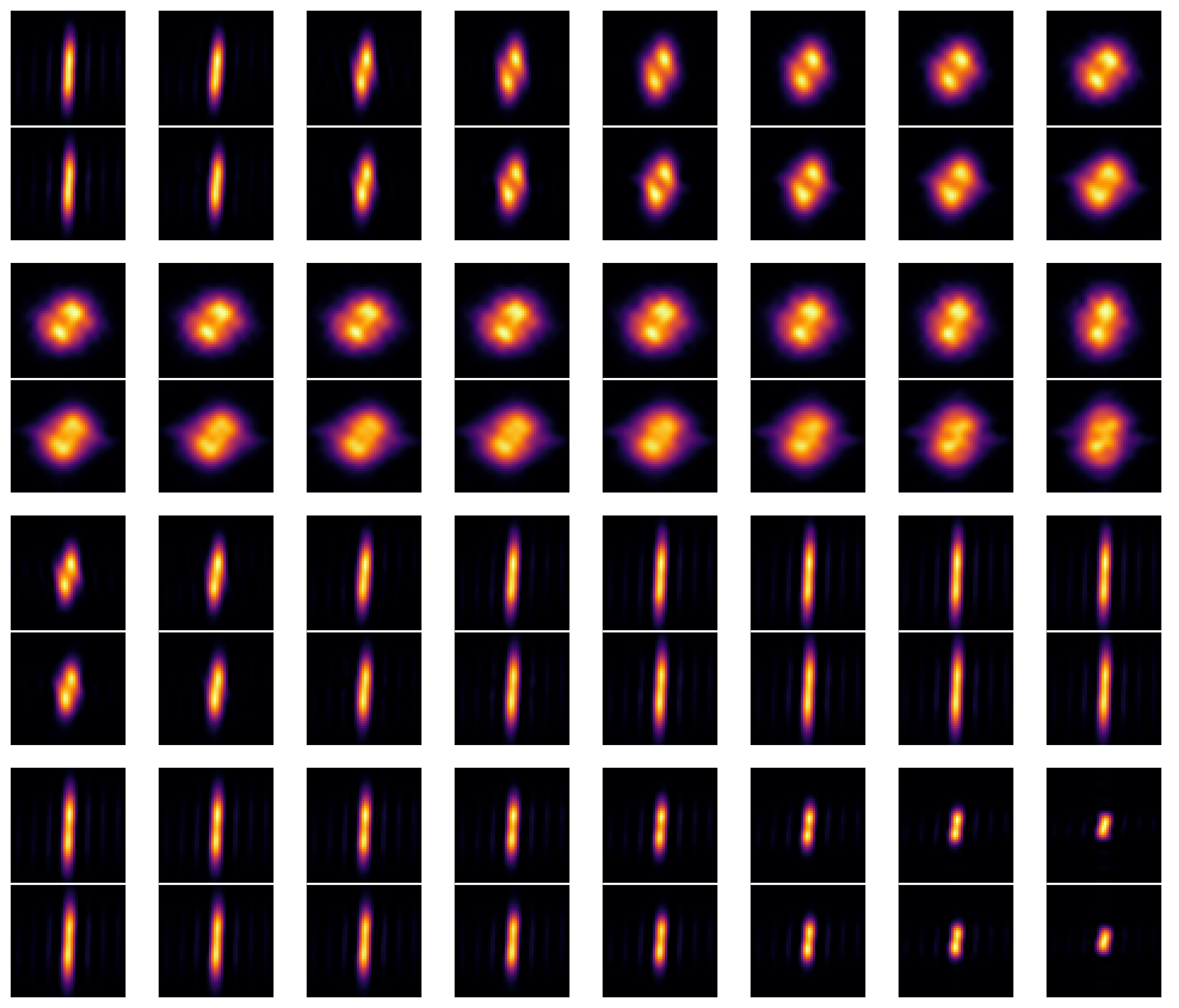
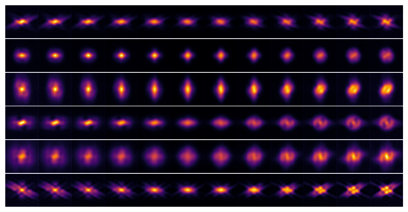
In using the latent space from the sinogram autoencoder to reconstruct the phase space distribution, it is implicitly assumed that smooth variations in the latent space parameters lead to smooth variations in the phase space distribution. If small changes in the latent space lead to large or abrupt changes in the phase space distribution, then it will be difficult to reconstruct the phase space distribution with any accuracy or reliability. The way in which we have constructed the sinogram autoencoder and phase space decoder does not guarantee that the phase space distribution has a smooth dependence on the latent space; however, it appears by inspection that the phase space distribution does in fact vary smoothly in response to continuous changes in the latent space parameters. An example, showing how two-dimensional projections of the four-dimensional phase space distribution vary in response to changes in the first latent space parameter, is shown in figure 11.
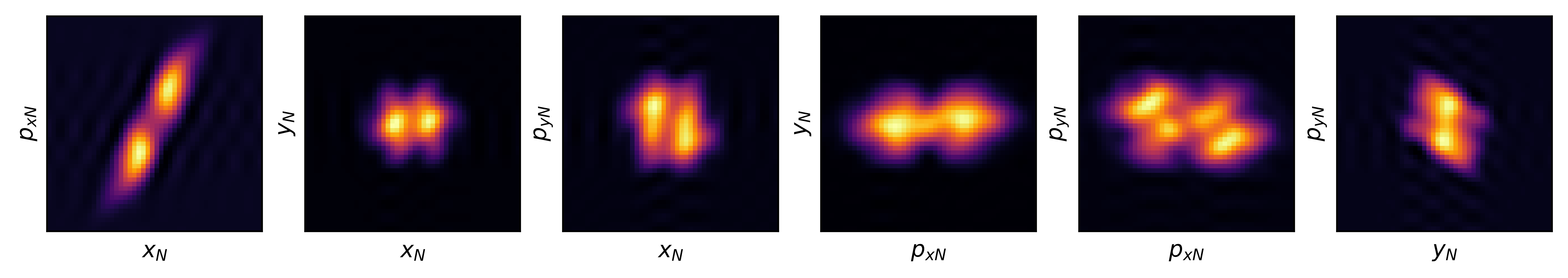
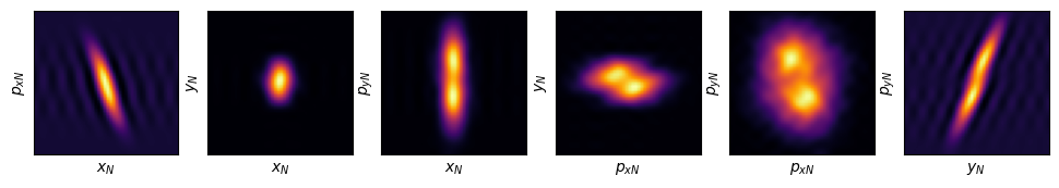
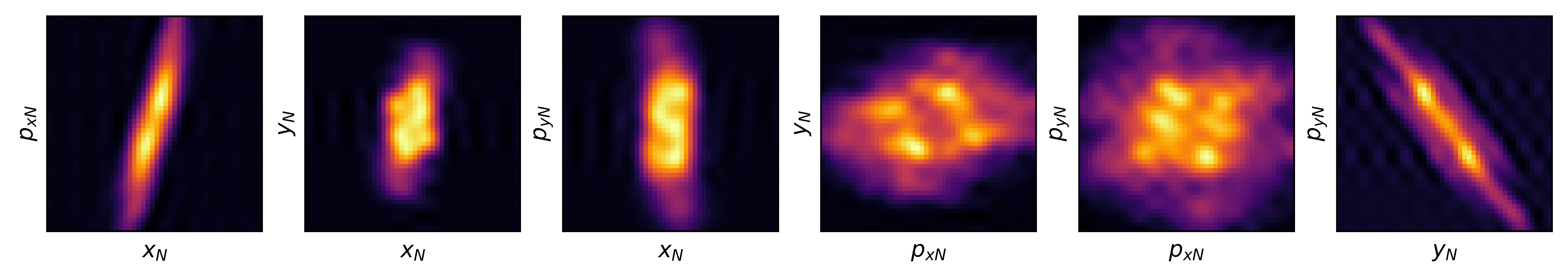
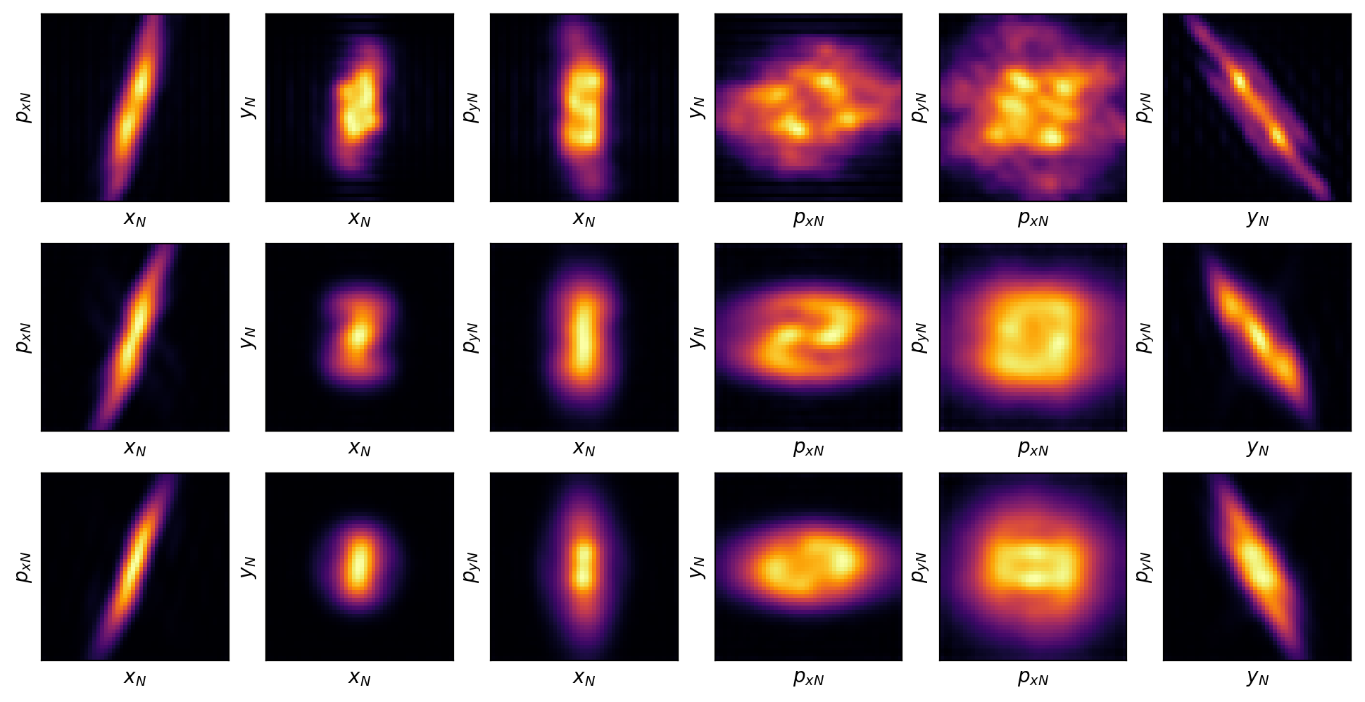
Some examples showing the performance of the phase space decoder are shown in figure 12. Three cases from the test data are shown: the top row in each case shows the ground truth (the phase space distribution used in simulation to construct the sinograms in the training data). The second row shows the reconstruction of the phase space distribution from the sinogram without errors, using the basic latent space from the sinogram autoencoder. The third row shows the reconstruction of the phase space distribution from the sinogram with quadrupole errors, using the extended encoder. The images in the second row illustrate how well the machine learning techniques presented here can reproduce the phase space distribution in the case of measurements without quadrupole errors. The images in the third row illustrate the performance of the machine learning techniques in the case of measurements in the presence of quadrupole errors. Although the reconstructed phase space distributions do not reproduce the full level of detail in the ‘true’ phase space distribution, the accuracy of the reconstruction in both cases (with or without quadrupole errors) is still good, even in the presence of quadrupole strength errors that significantly affect the sinograms (see figure 5).
Case A: quadrupole errors = (10.7%, -5.01%, -2.53%, 7.50%, 0.183%)
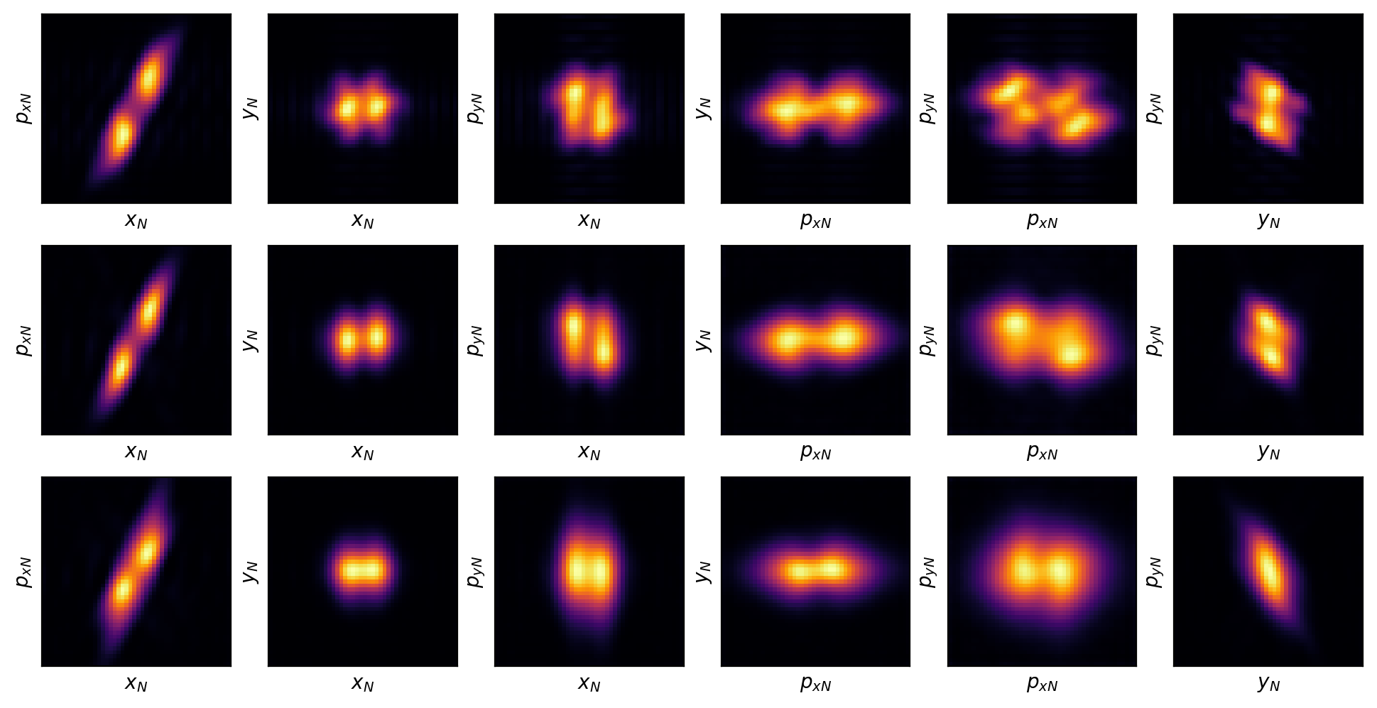
Case B: quadrupole errors = (-5.06%, -12.8%, 2.06%, 4.17%, -12.5%)
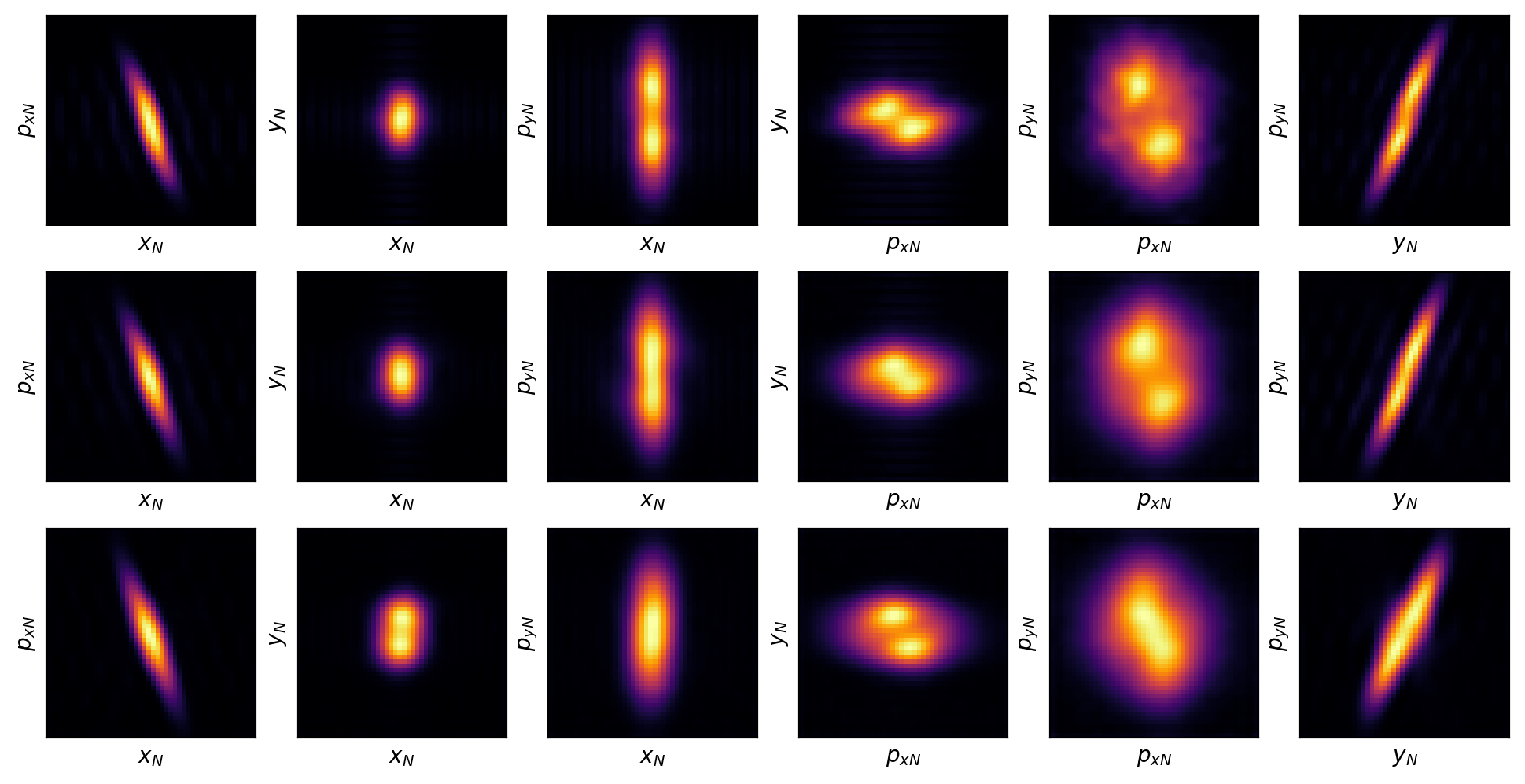
Case C: quadrupole errors = (3.89%, -11.9%, 8.89%, -4.81%, 14.0%)
4 Experimental demonstration
To demonstrate the application of the extended latent space technique for phase space tomography, we present some experimental results from CLARA. The data were collected in 2022, and a previous analysis was reported in [27]. The previous analysis used machine learning, but did not account for possible errors on the quadrupole strengths: the ML technique was based on a single neural network taking the DCT of a sinogram as input, and providing the DCT of the four-dimensional phase space distribution as output. The parameters (number of steps in the quadrupole scan, phase advances etc.) used for the examples shown in sections 2 and 3 in the current paper were chosen to allow the trained neural networks to be applied directly to the data from 2022. The data collected in 2022 included a case with bunch charge and a case with bunch charge . Here, we apply the new technique to the case with bunch charge : in the previous analysis [27], it proved more difficult to achieve good results with this data set, than for the case of a beam with lower () bunch charge.
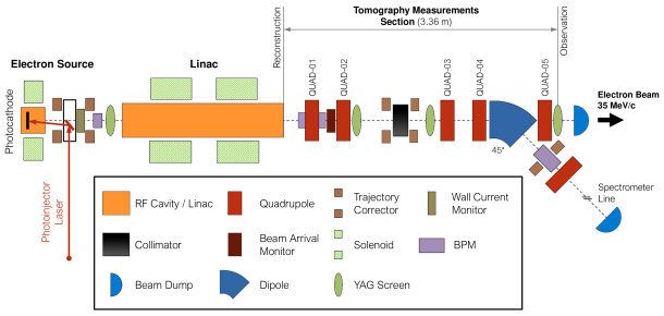
A schematic of CLARA including the section of beamline used for the tomography measurements is shown in figure 13. For the measurements, the machine was set up in a standard configuration with beam energy and bunch charge . The reconstruction and observation points are the end of the linac and the third diagnostics (YAG) screen following the linac, respectively. Five quadrupoles, labelled QUAD-01, QUAD-02, QUAD-03, QUAD-04 and QUAD-05 in figure 13 were used in the quadrupole scan.
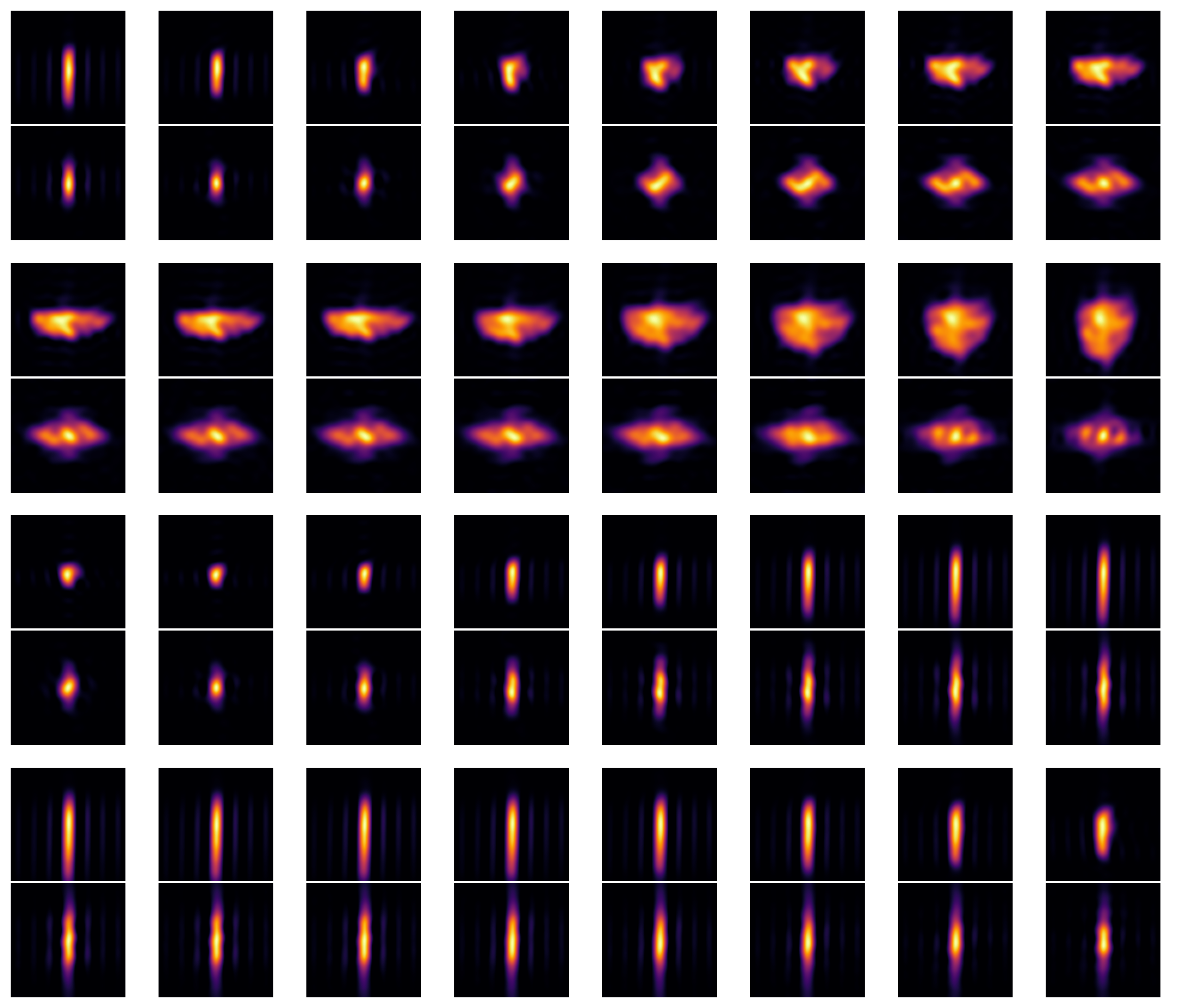
The screen images from the quadrupole scan are shown in figure 14, together with the output of the sinogram autoencoder. Note that the autoencoder does not take into account the possibility of errors on the quadrupole magnets. Although the autoencoder reproduces reasonably well the overall variation in the beam size over the course of the quadrupole scan, there are significant differences in individual images: this may indicate that experimental data were collected under conditions that do not accurately match the model used to construct the training data for the autoencoder. In other words, differences between the observed images and the images from the autoencoder may be the result of errors on components in the accelerator that are not taken into account in the simulation used to generate the training data.
The phase space reconstructed from the measured sinogram in CLARA is shown in figure 15. The top row in this figure shows projections (in normalised co-ordinates) of the phase space distribution found using the sinogram autoencoder and phase space decoder, i.e. without accounting for strength errors on the quadrupole magnets. The bottom row shows corresponding projections from the phase space distribution found using the extended encoder and phase space decoder, i.e. taking into account the effects of quadrupole strength errors. The projections in the top row of figure 15 can be compared with those of the previous analysis, shown in figure 12(b) in [27]. Despite some differences, there is general agreement in the shape of each projection.
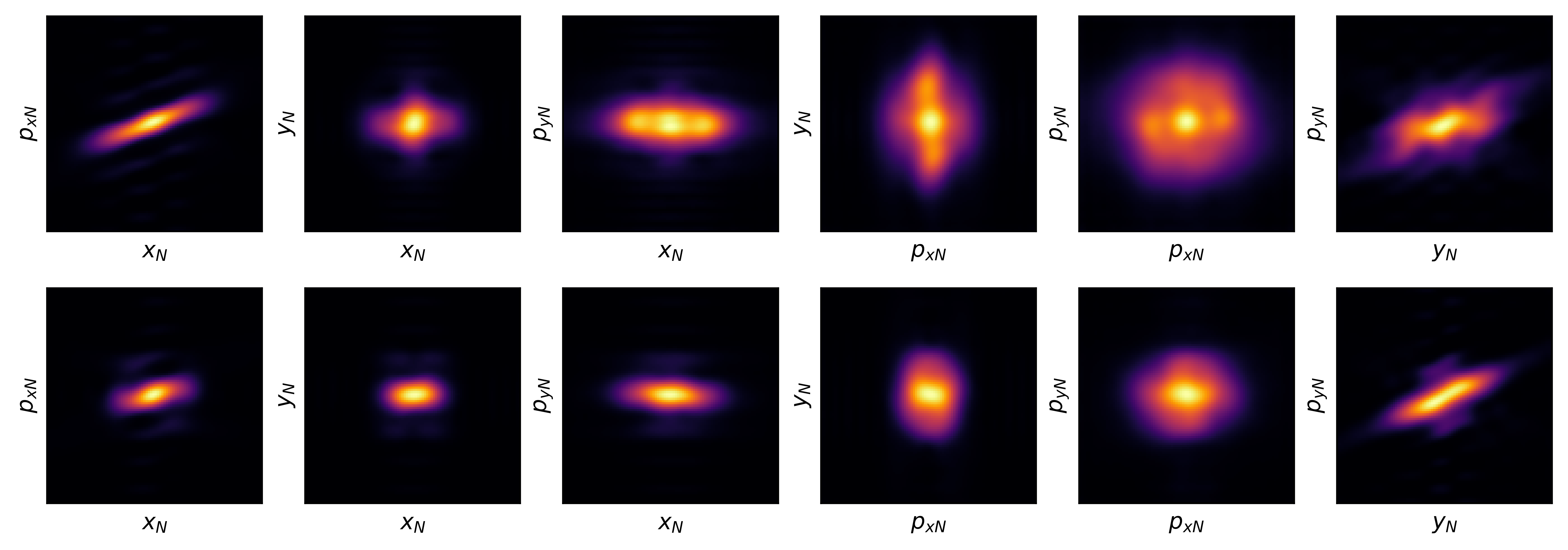
For the two distributions in figure 15, we observe that although the shapes of the distributions are similar, the distribution reconstructed using the extended encoder (taking quadrupole errors into account) appears to occupy a smaller volume in phase space than the distribution reconstructed using the sinogram autoencoder. For a Gaussian distribution, the emittance provides a convenient measure of the phase space volume occupied by a bunch of particles. To estimate the emittances, each of the distributions shown in figure 15 is fitted with a Gaussian of the form:
| (4.1) |
where is the covariance matrix for the four-dimensional Gaussian in normalised phase space (with phase space variables ), and is the peak density. The emittances can then be found from the covariance matrix using:
| (4.2) |
where are the emittances (with for each of the two normal modes in the transverse phase space), and the antisymmetric unit matrix is defined by:
| (4.3) |
The emittances thus found from the phase space distributions shown in figure 15 are given in table 1. Taking errors on the quadrupoles into account results in values for the beam emittances that are about a factor of 2 smaller than the values found without accounting for quadrupole errors.
| sinogram autoencoder | 8.0 m | 17.7 m |
|---|---|---|
| extended encoder | 4.8 m | 7.9 m |
As well as taking quadrupole focusing errors into account in reconstructing the phase space distribution, the extended encoder provides an indication of the sizes of the errors on the first three quadrupoles used in the quadrupole scan. For the CLARA data with bunch charge, the errors from the extended encoder are found to be (12.73.4)%, (12.72.8)% and (0.42.6)%. These errors are larger than would normally be expected; but it is worth noting that the first two quadrupoles have the same error values. The focusing errors in the quadrupoles may be the result of an error on the beam energy rather than an error in the field gradients (see the comments in section 3.1): the focusing strength of a quadrupole depends both on the field gradient in the magnet and on the energy of the beam. If, during collection of the experimental data, the beam energy was 10% below the energy assumed in the analysis, then the analysis would indicate an error of 10% on the gradient of a quadrupole in which the gradient was actually equal to the nominal gradient. In the present case, therefore, it is possible that the beam energy was about 12% below the expected value, while the first two quadrupoles had field gradients close to nominal. The third quadrupole, however, would then have a field gradient significantly lower than expected. Unfortunately, this possibility cannot be investigated further, because of subsequent changes to the accelerator made as part of work to upgrade the facility. However, although we do not present results in detail in this paper, an analysis (using the extended encoder) of the data for bunch charge suggests that the first two quadrupoles were close to their nominal focusing strengths, while the third quadrupole was weaker by roughly 10%. The results from the and cases would be consistent if it is assumed that the beam energy was lower than the nominal value for the measurements, close to nominal for the measurements, and that the third quadrupole had a gradient error of about -10% for both cases.
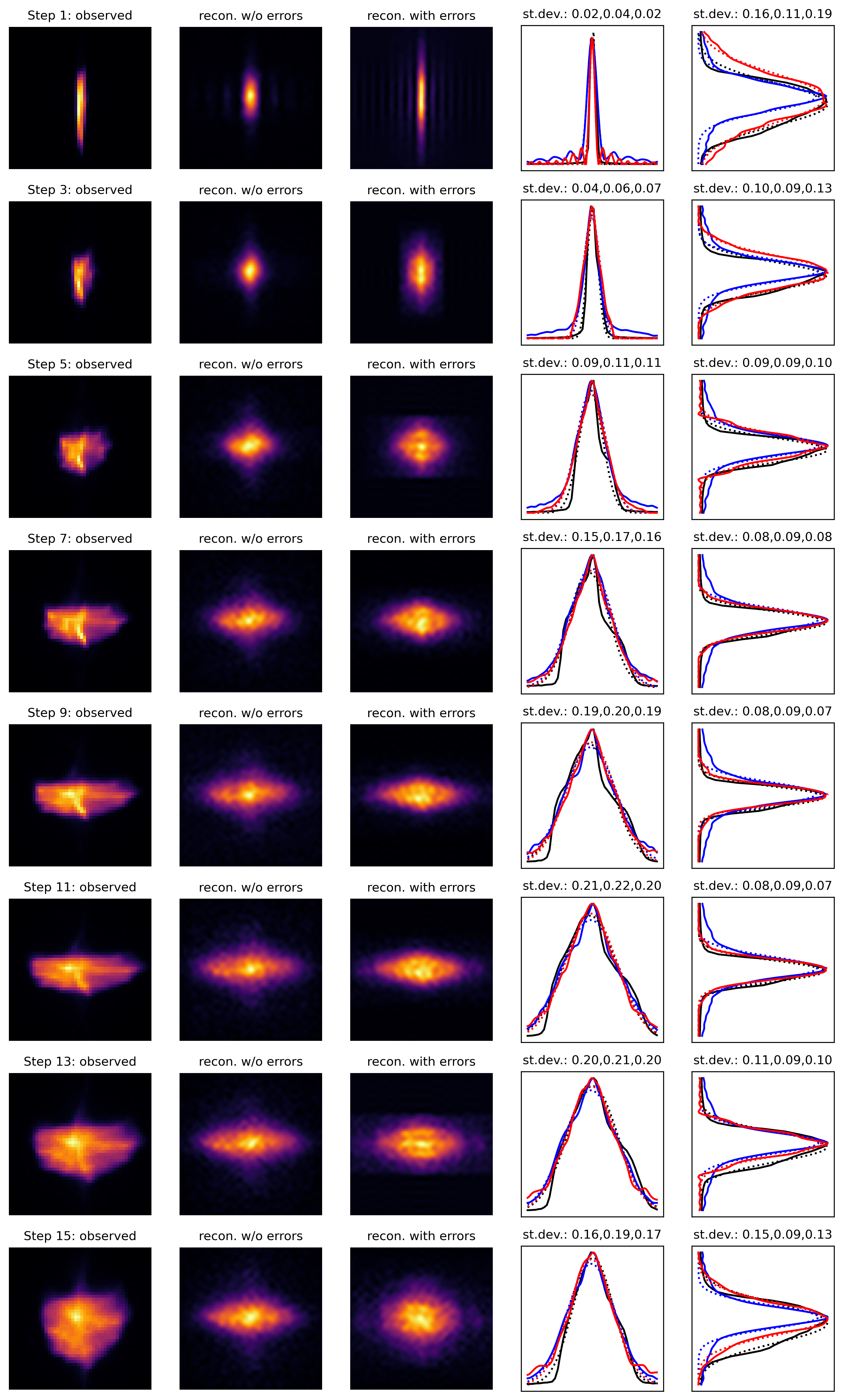
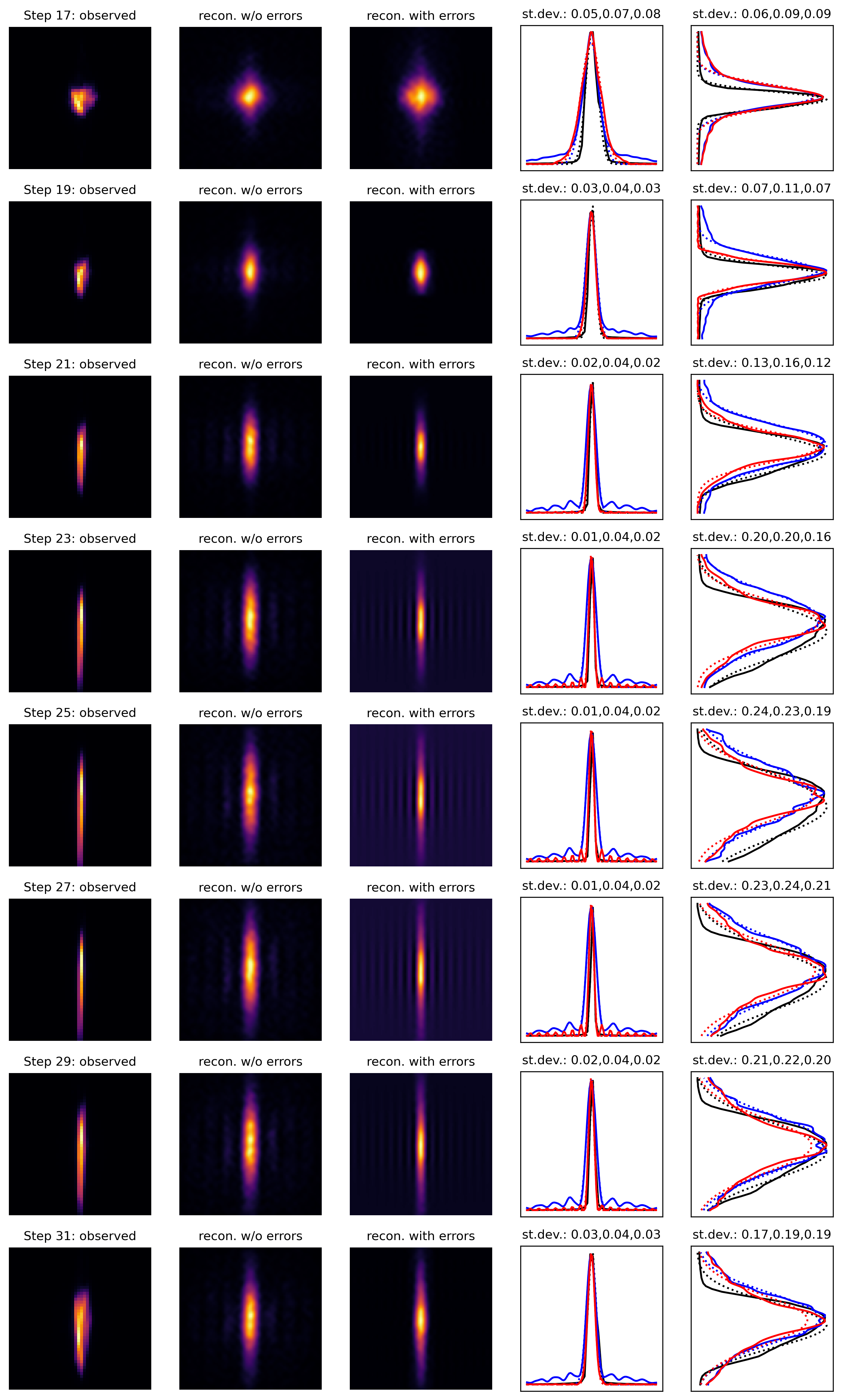
The reconstructed phase space distribution may be validated by comparing the screen images predicted by a tracking simulation (using the reconstructed phase space distribution and the estimated quadrupole strength errors) with the screen images observed during the measurements. Results of such a comparison are shown in figures 16 (for the first half of the quadrupole scan) and 17 (for the second half of the scan). Note that we show images from alternate steps in the quadrupole scan, rather than all 32 images. In these figures, the first three columns from left to right show: (1) the observed screen image; (2) the image reconstructed from the phase space decoder applied to the latent space from the sinogram autoencoder (i.e. neglecting quadrupole errors); (3) the image reconstructed from the phase space decoder applied to the extended latent space (i.e. accounting for quadrupole errors). The reconstructed images are from particle tracking simulations using the predicted phase space distributions, with quadrupole errors included for the images in the third column. The final two columns in figures 16 and 17 show projections of each image onto the horizontal and vertical axes, respectively. The solid black, blue and red lines correspond (respectively) to projections from the observed image, the reconstructed image neglecting quadrupole errors, and the reconstructed image accounting for quadrupole errors. Dotted lines show Gaussian fits, with standard deviations (as a fraction of the width of the image) shown in the text above each individual plot.
Although the machine learning methods that we have applied in the present analysis do not reveal the same level of detail in the phase space distribution as in the earlier work [27], we emphasise that a key feature of the technique presented here is the use of a low-dimensional latent space to allow the inclusion of parameters describing errors on accelerator components: some loss of detail is to be expected from reducing information about the phase space distribution to a set of just 40 parameters in the latent space.
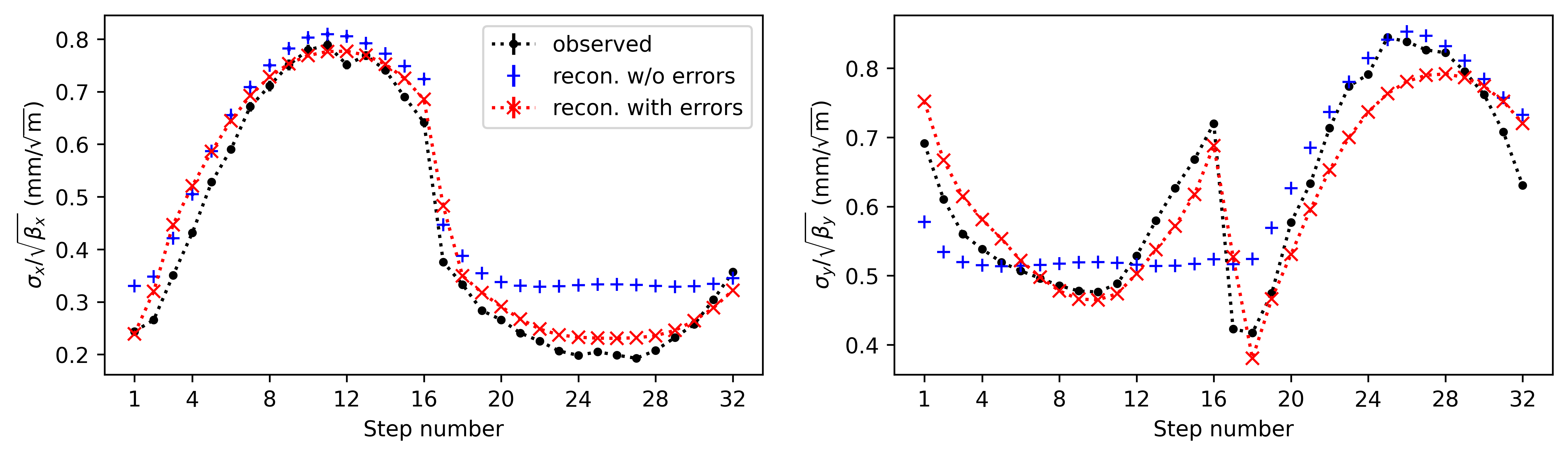
A simplified comparison between the observed screen images and the reconstructed images (neglecting or taking account of quadrupole errors) is presented in figure 18. The plots show the variation in horizontal and vertical beam sizes at the observation point over the course of the quadrupole scan, scaled by the square root of the beta function at the observation point (so that if the phase space distribution was correctly described by the lattice functions, the scaled beam size would be consant). The beam sizes are obtained from the widths of Gaussian fits to the projections of the respective screen images onto the horizontal and vertical axes. Although there are some differences between the observed and the reconstructed beam sizes, the overall level of agreement appears reasonable. The results in figure 18 can be compared with those shown in figure 14 in [27]. We see in particular that taking account of errors on the quadrupole magnets leads to significantly better agreement in the vertical beam size in steps 12 to 16 of the scan. Note, however, that the reconstruction without errors shown in figure 18 appears to given worse agreement (for some of the steps in the quadrupole scan) with the measured beam sizes than the results shown in figure 14 in [27]. Although we have not investigated the reasons in detail, it is possible that the previous analysis gave better agreement because of the way in which the neural network was designed to produce the phase space distribution directly, without an intermediate latent space. Without the dimensionality reduction resulting from the use of a latent space, the neural network would have greater flexibility to ‘fit’ the phase space distribution to the observed data even without taking advantage of the additional degrees of freedom allowed by explicit inclusion of quadrupole errors.
5 Conclusions
An increasing number of studies are demonstrating the value of machine learning techniques for accelerator diagnostics. Even where alternative methods for data analysis exist, machine learning can significantly reduce the time needed for processing complex data; but machine learning techniques can also make it possible to extend diagnostics tools beyond previous capabilities. For phase space tomography, there are well-established conventional algorithms that can be used, even in the case of higher-dimensional phase space reconstructions; but it is difficult, using these algorithms, to take account of machine errors. Given the complexity of accelerator systems, some variation of parameters (including magnet field strengths, RF field amplitudes and phases etc.) from their specified values is always possible; such variations can have a significant impact on beam behaviour, and it is therefore important to allow for the possibility of errors on components in an accelerator during any beam measurement. Machine learning techniques offer the possibility of taking account of machine errors in phase space tomography. Furthermore, once trained, a machine learning model can be used to reconstruct the phase space distribution in two degrees of freedom from a set of beam images much more quickly than by using conventional (non-ML) methods.
Taking advantage of the capabilities offered by machine learning can present some challenges. For example, for a technique involving supervised learning, there is the problem of generating or collecting sufficient training data. This often means depending on simulations, since for many problems it will not be possible to make a direct observation of the required output: this is the case, for example, in beam phase space tomography. Even where it is possible, in principle, to use experimental observations for training a machine learning model, the time required to collect sufficiently large data sets can make such an approach impractical.
A further challenge in the use of machine learning in accelerator diagnostics is validating the results. In the case of phase space tomography, it is possible to assess the accuracy of the reconstructed phase space distribution by simulating the measurements made in collecting the data, i.e. by reproducing the screen images. Ultimately, though, the most important test of any diagnostics measurement is whether the results are of value in tuning and operating the accelerator, which usually means being able to make accurate predictions, based on the diagnostics results, of the response of the accelerator to changes in the settings of different components.
The dependence in many cases on simulations for the application of machine learning techniques raises the importance of an accurate computer model of the accelerator. In this respect, a technique such as that presented in this paper (aiming to provide information about the accelerator components used in a measurement as well as the main goals of the measurement) can be of significant value, even if the information obtained about the measurement components is subject to some uncertainty. This is illustrated in the case of the CLARA data discussed in section 4, where taking some account of errors in accelerator components improves the match between the beam size variation observed during a quadrupole scan, and the variation predicted by the tomography results. Even though there remains some uncertainty regarding the (apparent) errors on the quadrupole focusing strengths, the analysis does provide some information that can be useful for further investigation and correction of possible errors.
Finally, as we observed in section 2, there are many different ways in which machine learning tools can be applied for phase space tomography. Understanding the most appropriate technique for a given problem, and optimizing the implementation (including the measurement parameters, machine learning architecture, and training data characteristics) is a formidable task, and will require further work.
Acknowledgments
We would like to thank our colleagues in STFC/ASTeC for help with the collection of experimental data, in particular Peter Williams, Boris Militsyn and Matthew King. This work was supported by STFC through a grant to the Cockcroft Institute.
References
- [1] C. Pellegrini and J. Stöhr, X-ray free-electron lasers—principles, properties and applications, Nucl. Instrum. Methods Phys. Res. A 500 (2003) 33.
- [2] B. McNeil and N. Thompson, X-ray free-electron lasers, Nature Photonics 4 (2010) 814.
- [3] W. Barletta, J. Bisognano, J. Corlett, P. Emma, Z. Huang, K.-J. Kim et al., Free electron lasers: Present status and future challenges, Nucl. Instrum. Methods Phys. Res. A 618 (2010) 69.
- [4] E.A. Seddon, J.A. Clarke, D.J. Dunning, C. Masciovecchio, C.J. Milne, F. Parmigiani et al., Short-wavelength free-electron laser sources and science: a review, Rep Prog Phys. 80 (2017) 115901.
- [5] M. Minty and F. Zimmermann, Measurement and control of charged particle beams, Springer, New York (2003).
- [6] E. Prat and M. Aiba, Four-dimensional transverse beam matrix measurement using the multiple-quadrupole scan technique, Phys. Rev. ST Accel. Beams 17 (2014) 052801.
- [7] C. McKee, P. O’Shea and J. Madey, Phase space tomography of relativistic electron beams, Nucl. Instrum. Methods Phys. Res. A 358 (1005) 264.
- [8] V. Yakimenko, M. Babzien, I. Ben-Zvi, R. Malone and X.-J. Wang, Electron beam phase-space measurement using a high-precision tomography technique, Phys. Rev. ST Accel. Beams 9 (2006) 112801.
- [9] D. Stratakis, R. Kishek, H. Li, S. Bernal, M. Walter, B. Quinn et al., Tomography as a diagnostic tool for phase space mapping of intense particle beams, Phys. Rev. ST Accel. Beams 6 (2003) 122801.
- [10] D. Stratakis, K. Tian, R. Kishek, I. Haber, M. Reiser and P. O’Shea, Tomographic phase-space mapping of intense particle beams using solenoids, Physics of Plasmas 14 (2007) 120703.
- [11] D. Xiang, Y.-C. Du, L.-X. Yan, R.-K. Li, W.-H. Huang, C.-X. Tang et al., Transverse phase space tomography using a solenoid applied to a thermal emittance measurement, Phys. Rev. ST Accel. Beams 12 (2009) 022801.
- [12] M. Röhrs, C. Gerth, H. Schlarb, B. Schmidt and P. Schmüser, Time-resolved electron beam phase space tomography at a soft x-ray free-electron laser, Phys. Rev. ST Accel. Beams 12 (2009) 050704.
- [13] Q. Xing, L. Du, X. Guan, C. Tang, M. Wang, X. Wang et al., Transverse profile tomography of a high current proton beam with a multi-wire scanner, Phys. Rev. Accel. Beams 21 (2018) 072801.
- [14] F. Ji, J.G. Navarro, P. Musumeci, D.B. Durham, A.M. Minor and D. Filippetto, Knife-edge based measurement of the 4d transverse phase space of electron beams with picometer-scale emittance, Phys. Rev. Accel. Beams 22 (2019) 082801.
- [15] K. Hock and A. Wolski, Tomographic reconstruction of the full 4d transverse phase space, Nucl. Instrum. Methods Phys. Res. A 726 (2013) 8.
- [16] A. Wolski, D.C. Christie, B.L. Militsyn, D.J. Scott and H. Kockelbergh, Transverse phase space characterization in an accelerator test facility, Phys. Rev. Accel. Beams 23 (2020) 032804.
- [17] D. Alesini, G.D. Pirro, L. Ficcadenti, A. Mostacci, L. Palumbo, J. Rosenzweig et al., Rf deflector design and measurements for the longitudinal and transverse phase space characterization at sparc, Nucl. Instrum. Methods Phys. Res. A 568 (2006) 488.
- [18] D. Marx, R. Assmann, P. Craievich, K. Floettmann, A. Grudiev and B. Marchetti, Simulation studies for characterizing ultrashort bunches using novel polarizable x-band transverse defection structures, Scientific Reports 9 (2019) 19912.
- [19] S.M. Jaster-Merz, R.W. Assmann, R. Brinkmann, F. Burkart, H. Dinter, F. Mayet et al., Characterization of the full transverse phase space of electron bunches at ARES, Proceedings of the 12th International Particle Acc. Conf., Campinas, SP, Brazil (2021) 952.
- [20] A. Scheinker, D. Filippetto and F. Cropp, 6d phase space diagnostics based on adaptively tuned physics-informed generative convolutional neural networks, Proceedings of the 13th International Particle Accelerator Conference, Bangkok, Thailand (2022) 776.
- [21] S.M. Jaster-Merz, R.W. Assmann, R. Brinkmann, F. Burkart and T. Vinatier, 5D tomography of electron bunches at ARES, Proceedings of the 13th International Particle Acc. Conf., Bangkok, Thailand (2022) 279.
- [22] S.M. Jaster-Merz, R.W. Assmann, R. Brinkmann, F. Burkart, W. Hillert, M. Stanitzki et al., 5D tomographic phase-space reconstruction of particle bunches, 2305.03538.
- [23] J. Frikel and E.T. Quinto, Characterization and reduction of artifacts in limited angle tomography, Inverse Problems 29 (2013) 125007.
- [24] K. Hock, M. Ibison, D. Holder, A. Wolski and B. Muratori, Beam tomography in transverse normalised phase space, Nucl. Instrum. Methods Phys. Res. A 642 (2011) 36.
- [25] B.T. Spiers, R. Aboushelbaya, Q. Feng, M.W. Mayr, I. Ouatu, R.W. Paddock et al., Methods for extremely sparse-angle proton tomography, Phys. Rev. E 104 (2021) 045201.
- [26] D. Marx, R. Assmann, P. Craievich, K. Floettmann, A. Grudiev and B. Marchetti, Deep learning for tomographic image reconstruction, Nature Machine Intelligence 2 (2020) 737.
- [27] A. Wolski, M.A. Johnson, M. King, B.L. Militsyn and P.H. Williams, Transverse phase space tomography in an accelerator test facility using image compression and machine learning, Phys. Rev. Accel. Beams 25 (2022) 122803.
- [28] K. Hwang, C. Mitchell and R. Ryne, Machine learning based phase space tomography using kicked beam turn-by-turn centroid data in a storage ring, Phys. Rev. Accel. Beams 26 (2023) 104601.
- [29] P. Baldi, K. Cranmer, T. Faucett, P. Sadowski and D. Whiteson, Parameterized neural networks for high-energy physics, Eur. Phys. J. C 76 (2016) 235.
- [30] R. Roussel, A. Edelen, C. Mayes, D. Ratner, J.P. Gonzalez-Aguilera, S. Kim et al., Phase space reconstruction from accelerator beam measurements using neural networks and differentiable simulations, Phys. Rev. Lett. 130 (2023) 145001.
- [31] A. Scheinker, Adaptive machine learning for time-varying systems: low dimensional latent space tuning, JINST 16 (2021) P10008.
- [32] A. Scheinker, F. Cropp, S. Paiagua and D. Filippetto, An adaptive approach to machine learning for compact particle accelerators, Scientific Reports 11 (2021) 19187.
- [33] A. Scheinker, F. Cropp and D. Filippetto, Adaptive autoencoder latent space tuning for more robust machine learning beyond the training set for six-dimensional phase space diagnostics of a time-varying ultrafast electron-diffraction compact accelerator, Phys. Rev. E 107 (2023) 045302.
- [34] R. Roussel, A. Edelen, C. Mayes, D. Ratner, J.P. Gonzalez-Aguilera, S. Kim et al., Phase space reconstruction from accelerator beam measurements using neural networks and differentiable simulations, 2209.04505.
- [35] D. Angal-Kalinin, A. Brynes, R. Buckley, S. Buckley, R. Cash, H.C. Cortes et al., Status of CLARA front end commissioning and first user experiments, Proceedings of the 10th International Particle Accelerator Conference, Melbourne, Australia (2019) 1851.
- [36] D. Angal-Kalinin, A. Bainbridge, A.D. Brynes, R.K. Buckley, S.R. Buckley, G.C. Burt et al., Design, specifications, and first beam measurements of the compact linear accelerator for research and applications front end, Phys. Rev. Accel. Beams 23 (2020) 044801.
- [37] N. Ahmed, T. Natarajan and K.R. Rao, Discrete cosine transform, IEEE Transactions on Computers C-23 (1974) 90.
- [38] W.-H. Chen and W. Pratt, Scene adaptive coder, IEEE Transactions on Communications 32 (1984) 225.
- [39] K.R. Rao and P. Yip, Discrete cosine transform: algorithms, advantages, applications, Academic Press, San Diego, CA, USA (1990), DOI:10.1016/C2009-0-22279-3.
- [40] M.A. Kramer, Nonlinear principal component analysis using autoassociative neural networks, AIChE Journal 37 (1991) 233 [https://aiche.onlinelibrary.wiley.com/doi/pdf/10.1002/aic.690370209].
- [41] F. Chollet et al., “Keras.” https://keras.io, 2015.
- [42] A. Krogh and J.A. Hertz, A simple weight decay can improve generalization, in Neural Information Processing Systems, 1991, https://api.semanticscholar.org/CorpusID:10137788.
- [43] “Keras 3 API documentation / Layers API / Layer activation functions.” https://keras.io/api/layers/activations/.