Anomalous radial acceleration of galaxies and clusters supports hyperconical modified gravity

Abstract

General relativity (GR) is the most successful theory of gravity, with great observational support at local scales. However, to keep GR valid at over cosmic scales, some phenomena (such as the flat galaxy rotation curves and the cosmic acceleration) require the assumption of exotic dark matter. The radial acceleration relation (RAR) indicates a tight correlation between dynamical mass and baryonic mass in galaxies and galaxy clusters. This suggests that the observations could be better explained by modified gravity theories without exotic matter. Modified Newtonian Dynamics (MOND) is an alternative theory for explaining some cases of flat galaxy rotation curves by using a new fundamental constant acceleration $a_{0}$, the so-called Milgromian parameter. However, this non-relativistic model is too rigid (with insufficient parameters) to fit the large diversity of observational phenomena. In contrast, a relativistic MOND-like gravity naturally emerges from the hyperconical model, which derives a fictitious acceleration compatible with observations. This study analyzes the compatibility of the hyperconical model with respect to RAR observations of 10 galaxy clusters obtained from HIFLUGCS and 60 high-quality SPARC galaxy rotation curves. The results show that a general relation can be fitted to most cases with only one or two parameters, with an acceptable chi-square and $p$-value. These findings suggest a possible way to complete the proposed modification of GR on a cosmic scale.

revtex4-1Repair the float hyperrefOption hyperrefToken pdftex(dest) namerefThe TS1aercmr

1 Introduction

1.1 The dark matter missing gravity problem

As is well known, observational tests of General Relativity (GR) show successful results on Solar System scales (Dittus & Lämmerzahl, 2007; Ciufolini et al., 2019; Touboul et al., 2022; Liu et al., 2022; Desmond et al., 2024; Vokrouhlický et al., 2024). The good skill of standard gravity seems to be in question only on larger scales (Chae et al., 2020; Banik & Zhao, 2022). It is well-known that exotic cold dark matter (CDM) is required to extend GR to cosmic scales. However, the not-yet-discovered CDM particles present strong theoretical challenges, such as explaining the tight empirical relationship between observed gravitational anomalies (assimilated to CDM) and the distribution of visible baryonic matter in galaxies (Trippe, 2014; Merritt, 2017; Goddy et al., 2023). This empirical law is known as the mass-discrepancy acceleration relation (McGaugh, 2004; Di Cintio & Lelli, 2015; Desmond, 2016, MDAR,), the mass-luminosity relation (Leauthaud et al., 2010; Cattaneo et al., 2014), the baryonic Tully-Fisher relation (Lelli et al., 2019; Goddy et al., 2023, BTFR,), or the more general radial acceleration relation (McGaugh et al., 2016; Lelli et al., 2017; Tian et al., 2020, RAR;).

Tian et al. (2020) found that the observed RAR in galaxy clusters is consistent with predictions from a semi-analytical model developed in the standard Lambda-CDM ($\Lambda$CDM) framework. To explain how the contribution of CDM is determined by that of baryons, some authors suggest that they present a strong coupling that leads to an effective law such as the MDAR/BTFR/RAR (Blanchet, 2007; Katz et al., 2016; Barkana, 2018).

However, the lack of direct detection (or indirect non-gravitational) of dark matter suggests a weak or even non-existent coupling between CDM and baryons (Abel et al., 2017; Hoof et al., 2020; Du et al., 2022; Aalbers et al., 2023; Hu et al., 2024), which is in conflict with these empirical relationships. Moreover, excess rotation occurs only where the Newtonian acceleration $a_{N}$ induced by the visible matter is lower than a typical scale of about $a_{N}\lesssim a_{0}\approx 1.2\times 10^{-10}\mathrm{m\,s}^{-2}$, suggesting that it is a space-time problem rather than a matter-type problem. This is also consistent with the deficient dark-matter halos that some relic galaxies (above of the $a_{0}$ scale) seem to indicate (Comerón et al., 2023). In other cases, the CDM halo hypothesis also predicts a systematically deviating relation from the observations, with densities about half of what is predicted by CDM simulations (de Blok et al., 2008), while the rotation curves appear to be more naturally explained by modified gravity (McGaugh et al., 2007, 2016; Famaey & McGaugh, 2012; Banik & Zhao, 2022; Chae, 2022).

The hypothesis of ‘dark matter’ also presents difficulties in explaining some phenomena such as the absence of the expected Chandrasekhar dynamical friction in cluster collisions, falsified by more than 7 sigmas (Kroupa, 2015; Ardi & Baumgardt, 2020; Kroupa et al., 2023). The lack of dynamical friction on galaxy bars is a strong argument that the central density of CDM in typical disc galaxies has to be a lot smaller than expected in standard CDM simulations (Roshan et al., 2021). Another example is the morphology of dwarf galaxies. According to Asencio et al. (2022), observed deformations of dwarf galaxies in the Fornax Cluster and the lack of low-surface-brightness dwarfs toward its center are incompatible with $\Lambda$CDM predictions. Moreover, the dwarfs analyzed in that study have sufficiently little stellar mass that the observations cannot be explained by baryonic feedback effects, but they are consistent with the Milgromian modified Newtonian dynamics (Milgrom, 1983, MOND;). Therefore, most observations suggest the need to explore modified gravity as an alternative to the standard model (Trippe, 2014; Merritt, 2017).

1.2 Beyond the MOND paradigm

The MOND paradigm has been deeply explored, from galactic dynamics to the Hubble tension, which is explained by a more efficient (early) formation of large structures such as the local supervoid (Keenan et al., 2013; Haslbauer et al., 2020; Banik & Zhao, 2022; Mazurenko et al., 2023). In fact, RAR has been thoroughly analyzed for galaxy rotation curves collected from the Spitzer Photometry and Accurate Rotation Curves (SPARC) sample (Lelli et al., 2016, 2019). The results were anticipated over three decades ago by MOND (Milgrom, 1983; McGaugh et al., 2016), although the form of the transition between the Newtonian and Milgromian regimes must be found empirically.

However, the relativistic formulation of MOND was less successful. In particular, Bekenstein proposed a non-cosmological version of Tensor-Vector-Scalar (TeVeS) gravity (Bekenstein, 2004; Famaey & McGaugh, 2012) that predicts unstable stars on a scale of a few weeks (Seifert, 2007), which is only avoidable with an undetermined number of terms (Mavromatos et al., 2009). To solve these issues, Skordis & Złośnik (2021) found that, by adding terms analogous to the FLRW action, at least the second-order expansion is free of ghost instabilities. Their model is also capable of obtaining gravitational waves traveling at the speed of light $c$, which was not the case with the original TeVeS. However, the authors pointed out that it needs to be embedded in a more fundamental theory.

Recently, Blanchet & Skordis (2024) proposed a relativistic MOND formulation based on space-time foliation by three-dimensional space-like hypersurfaces labeled by the Khronon scalar field. The idea is very similar to the Arnowitt–Deser–Misner (ADM) treatment in the dynamical embedding of the hyperconical universe (Monjo, 2017, 2018; Monjo & Campoamor-Stursberg, 2020; Monjo, 2023, 2024a, 2024b).

Applying perturbation theory to the hyperconical metric, a relativistic theory with MOND phenomenology is obtained, which fits adequately to 123 SPARC galaxy rotation curves (Monjo, 2023). The cosmic acceleration derived from it is $a_{\gamma 0}:=2\gamma_{0}^{-1}c/t$, where $t$ is the age of the universe, $c$ is the speed of light, and $\gamma_{0}>1$ is a projection parameter that translates from the ambient spacetime to the embedded manifold (Monjo & Campoamor-Stursberg, 2023; Monjo, 2024a). In contrast to the Milgrom constant $a_{0}$, the cosmic acceleration $a_{\gamma 0}$ is a variable that depends on the geometry considered (mainly the ratio between escape speed and Hubble flux). The equivalence between the $a_{0}$ and $a_{\gamma 0}$ scales is found for $\gamma_{0}\approx 13\pm 3$.

In the limit of weak gravitational fields and low velocities, the hyperconical model is also linked to the scalar tensor vector gravity (STVG) theory, popularly known as Moffat’s modified gravity (MOG). The MOG/STVG model is a fully covariant Lorentz invariant theory that includes a dynamical massive vector field and scalar fields to modify GR with a dynamical ‘gravitational constant’$G\,$ (Moffat & Toth, 2009, 2013; Harikumar & Biesiada, 2022). In particular, it leads to an anomalous acceleration of about $2\,{G}\alpha_{G}D^{2}\,\approx\,1.1\times 10^{-10}\mathrm{m\,s}^{-2}\,\approx\,2\gamma_{0}^{-1}c/t$ for $\gamma_{0}\approx 12$, with $\alpha_{G}\approx 10$ and the universal MOG constant $D=6.25\times 10^{3}M_{\odot}^{1/2}\;\mathrm{kpc}^{-1}$. Fixing these parameters by using galaxy rotation curves, MOG fails to account for the observed velocity dispersion profile of Dragonfly 44 at 5.5 sigma confidence even if one allows plausible variations to its star formation history and thus stellar mass-to-light ratio:

The number of parameters needed to accommodate most theories to the observations of galaxy clusters is perhaps too large and unnatural. In all cases, the phenomenological parameters (e.g., the CDM distribution profile, the ad-hoc MOND interpolating function $\mu$, and the MOG constant $D$) need additional theoretical motivation. In contrast, the hyperconical model proposed by Monjo derives a natural modification of GR from minimal dynamical embedding in a (flat) five-dimensional Minkowskian spacetime (Monjo, 2023, 2024a, 2024b).

Therefore, this Letter aims to show how the anomalous RAR of ten galaxy clusters, analyzed by Eckert et al. (2022) and Li et al. (2023), are adequately modeled by the hyperconical modified gravity (HMG) of Monjo (2023). As Tian et al. (2020) pointed out, clusters present a larger anomalous acceleration ($g\sim 10^{-9}\mathrm{m\,s}^{-2}$) than galaxy rotation curves ($g\sim 10^{-10}\mathrm{m\,s}^{-2}$), reflecting the missing baryon problem that remains a challenge for MOND in galaxy clusters (Famaey & McGaugh, 2012; Li et al., 2023; Tian et al., 2024). This open issue is addressed here with the following structure: Sect. 2 summarizes the data used and the HMG model; Sect. 3 shows the main results in the fits and discusses predictions for galaxies and smaller systems, and finally Sect. 4 points out the most important findings and concluding remarks.

2 Data and model

2.1 Observations used

This study uses observational estimates of the radial acceleration relations (RAR; total gravity observed compared to Newtonian gravity due to baryons) for 10 galaxy clusters ($0.0328<z<0.0899$) that were collected from the HIghest X-ray FLUx Galaxy Cluster Sample (Li et al., 2023, HIFLUGCS,). In particular, the galaxy clusters considered are as follows: A0085, A1795, A2029, A2142, A3158, A0262, A2589, A3571, A0576, A0496. Moreover, to compare our results, rotation curves were collected from 60 high-quality SPARC galaxies filtered to well-measured intermediate radii (McGaugh et al., 2007, 2016; Lelli et al., 2019).

2.2 Radial acceleration from hyperconical modified gravity (HMG)

Observations were used to assess whether the empirical RAR is in agreement with HMG as developed by Monjo (2023) and summarized here. Let $g$ be the background metric of the so-called hyperconical universe (Monjo, 2017, 2018; Monjo & Campoamor-Stursberg, 2020, 2023). The metric $g$ is locally approximately given by

$$g\approx dt^{2}\left(1-kr^{\prime 2}\right)-\frac{t^{2}}{t_{0}^{2}}\left(\frac{dr^{\prime 2}}{1-kr^{\prime 2}}+{r^{\prime}}^{2}d{\Sigma}^{2}\right)-\;\;\frac{2r^{\prime}t}{t_{0}^{2}}\frac{dr^{\prime}dt}{\sqrt{1-kr^{\prime 2}}}\,,{}$$ (1)

where $k=1/t_{0}^{2}$ is the spatial curvature for the current value $t_{0}\equiv 1$ of the age $t$ of the universe, while $t/{t_{0}}$ is a linear scale factor (Monjo, 2024a), $r^{\prime}\ll t_{0}$ is the comoving distance, and $\Sigma$ represents the angular coordinates. The shift and lapse terms of Eq. 1 lead to an apparent radial spatial inhomogeneity that is assimilated as a fictitious acceleration with adequate stereographic projection coordinates, which is a candidate to explain the Hubble tension (Monjo & Campoamor-Stursberg, 2023).

On the other hand, any gravitational system of mass $M_{sys}$ generates a perturbation over the background metric $g\to\hat{g}$ (Eq. 1) such that $k{r^{\prime 2}}\to\hat{k}{{\hat{r}}^{\prime 2}}:=k{{\hat{r}}^{\prime 2}}+{2{G}M_{sys}}/{{\hat{r}}^{\prime}}$. Applying local validity of GR (Appendix A), the perturbation term $\hat{h}:=\hat{g}-g$ is a key of the model (Appendix B). Another key is the stereographic projection of the coordinates $r^{\prime}\to{\hat{r}}^{\prime}=\lambda^{1/2}r^{\prime}$ and $t\to\hat{t}=\lambda t$, given by a scaling factor $\lambda:=1/(1-\gamma/\gamma_{0})$ that is a function of the angular position $\gamma=\sin^{-1}(r^{\prime}/t_{0})$ and a projection factor $\gamma_{0}^{-1}=\gamma_{sys}^{-1}\cos\gamma_{sys}$, where $\gamma_{sys}$ is the characteristic angle of the gravitational system (Appendix C). In an empty universe, $\gamma_{0}=\gamma_{U}/\cos\gamma_{U}$. We expect $\gamma_{U}=\frac{1}{3}\mathrm{\pi}$ and therefore that $\gamma_{0}=\frac{2}{3}\mathrm{\pi}\approx 2$; while the projective factor of maximum causality, $\gamma_{0}^{-1}=1$, arises for $\gamma_{U}\approx 0.235\mathrm{\pi}$ as then $\gamma_{U}=\cos\gamma_{U}$.

When geodesic equations are applied to the projected time component of the perturbation $\hat{h}_{tt}$, a fictitious cosmic acceleration of roughly $\gamma_{0}^{-1}c/t$ emerges in the spatial direction (see Appendix C.3):

$$\frac{|a_{Tot}-a_{N}|}{c/t}\approx\frac{1}{\gamma_{0}}\approx\frac{\cos\gamma_{sys}}{\gamma_{sys}}\,,$$ (2)

where $a_{N}:={G}M_{sys}/r^{2}$ is the Newtonian acceleration. However, a time-like component is also found in the acceleration that contributes to the total centrifugal acceleration $a_{C}$ such that $a_{C}\approx\sqrt{a_{N}^{2}+{2c}/(\gamma_{0}t)}$, which is useful to model galaxy rotation curves under the HMG framework (Monjo, 2023). Alternatively to Eq. 2, the cluster RAR is usually expressed as a quotient between total and Newtonian acceleration. That is,

$$\frac{a_{Tot}}{a_{N}}\approx 1-\frac{c}{a_{N}\gamma_{0}t}\,,$$ (3)

with factor $\gamma_{0}^{-1}=\gamma_{sys}^{-1}\cos\gamma_{sys}$, where the projective angle $\gamma_{sys}$ can be estimated from the galaxy cluster approach (Eq. C5) or from the general model (Eq. C3), respectively, by considering the relative geometry (angle) between the Hubble speed $v_{H}:=r/t$ and the Newtonian circular speed $v_{C}:=\sqrt{{G}M_{sys}/r}$ or its classical escape velocity $v_{E}:=\sqrt{2}\,v_{C}$, as follows:

$$\sin^{2}\gamma_{cluster}(r)\;\;\; \approx \;\;\;\sin^{2}\gamma_{galaxy}-\left({\sin^{2}\gamma_{galaxy}-\sin^{2}\gamma_{U}}\right)\frac{v_{E}^{2}(r)}{\varepsilon^{2}_{H}v_{H}^{2}(r)+v_{E}^{2}(r)}\;,\hskip 14.22636pt$$ (4)

$$\sin^{2}\gamma_{cluster}(r)\;\;\; \approx \;\;\;\sin^{2}\gamma_{U}+\left({\sin^{2}\gamma_{center}-\sin^{2}\gamma_{U}}\right)\bigg{|}\frac{v_{E}^{2}(r)-\epsilon^{2}_{H}v_{H}^{2}(r)}{v_{E}^{2}(r)+\epsilon^{2}_{H}v_{H}^{2}(r)}\bigg{|}\;,$$ (5)

where the parameter $\epsilon^{2}_{H}$ is the so-called relative density of the neighborhood (Appendix C.1), while $\gamma_{center}=\mathrm{\pi}/2$ and $\gamma_{U}=\mathrm{\pi}/3$ or $\gamma_{U}\approx 0.235\mathrm{\pi}$ can be fixed here to set a 1-parameter ($\epsilon_{H}$) general model from Eq. 5. As a second-order approach, this study also assumes that $\{\epsilon_{H},\gamma_{galaxy}\}$ can be free in our 2-parameter model for clusters (Eq. 4).

3 Results and discussion

3.1 Fitted values

Individually, fitting of Eq. 4 for the quotient between total and Newtonian acceleration (Eq. 3) leads to a square root of the relative density of about $\varepsilon_{H}=38^{+29}_{-11}$ (90% confidence level; Appendix C.4, Fig. C.2). Using the specific model for the clusters (Eq. 4), all fits provide an acceptable $\chi^{2}$ ($p$-value $<0.667$) except for the A2029 cluster, which did not pass the $\chi^{2}$ test for the fixed neighborhood projective angle of $\gamma_{0}=2$ (i.e., $\gamma_{U}=\mathrm{\pi}/3$). However, it did for $\gamma_{0}=1$ (i.e., $\gamma_{U}\approx 0.235\mathrm{\pi}$), which implies to use the causality limit for the cosmic acceleration instead of the empty-space limit.

Globally, the correlation of RAR values (differences) with respect to the escape-Hubble approach (Eqs. 2 and 4) is slightly higher ($R^{2}=0.83$) than with respect to the Newtonian acceleration ($R^{2}=0.79$). The simplest model of fixing $\gamma_{U}=\mathrm{\pi}/3$ and using a single global parameter, $\varepsilon_{H}=40_{-6}^{+8}$, gives a Pearson coefficient of $R^{2}=0.75$, while if $\gamma_{U}=\mathrm{\pi}/3$ is replaced by $\gamma_{U}=0.235\mathrm{\pi}$, we get instead $R^{2}=0.83$ with $\varepsilon_{H}=60_{-8}^{+20}$ (90% confidence level).

Larger anomalies in acceleration are found for the higher escape speeds ($v_{E}/v_{H}\sim\varepsilon_{H}$) in clusters. However, this is the opposite for galaxies, which experience the maximum anomaly for low escape velocities ($v_{E}/v_{H}<\varepsilon_{H}$), as shown in Fig. 1. In clusters, the relative density between the dominant galaxy (BCG) and the neighborhood determines this opposite behavior. The value of $v_{E}/v_{H}\sim\varepsilon_{H}$ points to the transition regime between small and large anomalies.

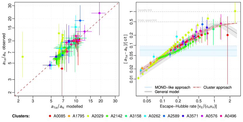
Figure 1: RAR modelling with HMG for total acceleration ($a_{Tot}$) compared to Newtonian acceleration ($a_{N}$). Left: Individual fitting (Eqs. 3 and 4) for the galaxy clusters considered (Li et al., 2023) with two parameters ($\varepsilon_{H}$ and $\gamma_{galaxy}$; Table 1). Right: Global fitting for all data according to three models: MOND-like constant (blue band), general model (gray band, Eqs. 2 and 5), and the cluster model (red band, Eqs. 2 and 4). The MOND-like model with constant $\gamma_{0}^{-1}=\gamma_{sys}^{-1}\cos\gamma_{sys}$ was considered with $\gamma_{sys}=0.466^{+0.011}_{-0.01}\mathrm{\pi}$, which corresponds to a Milgrom’s constant of $a_{0}=2\gamma_{0}^{-1}c/t=1.01_{-0.32}^{+0.33}\times 10^{-10}\mathrm{m\,s}^{-2}$ (Monjo, 2023). In the right panel, both the general model and the specific approach for clusters use only one free parameter ($\varepsilon_{H}$), by setting the projective angle of galaxies as $\gamma_{galaxy}=\mathrm{\pi}/2$ and $\gamma_{U}=\mathrm{\pi}/3$: The general model (gray band) is represented by the value of $\varepsilon_{H}=56_{-12}^{+22}$, while the cluster approach (red band) considers an average of $\varepsilon_{H}=40_{-6}^{+8}$. The shaded areas represent the 90% confidence interval.

3.2 Predictions for galaxy dynamics

As discussed in Sect. 1, HMG derives a relationship between the Milgrom acceleration $a_{0}\approx 1.2\times 10^{-10}\text{m/s}^{2}$ and the cosmic parameter $c/t\approx 6.9\times 10^{-10}\text{m/s}^{2}$, since $a_{0}\approx a_{\gamma 0}:=2\gamma_{0}^{-1}c/t$ for galaxy rotation curves, for an approximately constant $\gamma_{0}^{-1}\approx 0.08$ (Monjo, 2023). However, the geometry of gravitational systems led to a variable value of the projection factor $\gamma_{0}^{-1}\in(0,1)$, depending on the ration between escape speed and Hubble flux.

According to the general model of projective angles (Eq. 5), it is expected that galaxies and galaxy clusters exhibit opposite behaviors, but following the same theoretical curve. Using $\gamma_{center}=\mathrm{\pi}/2$, $\gamma_{U}=\mathrm{\pi}/3$, and $\varepsilon_{H}=56_{-12}^{+22}$ (obtained from the cluster data), we apply Eqs. 2 and 5 to predict the behavior of 60 galaxies, whose data were collected by McGaugh et al. (2007). By directly applying Eq. 5 to the escape speed of galaxies, a relative anomaly of $(a_{Tot}-a_{N})/(c/t)=\gamma_{0}^{-1}$ between $0.05$ and $0.40$ is predicted, close to the observations of $\gamma_{0}^{-1}=0.07_{-0.02}^{+0.03}$ in the galaxy rotation curves.

The wide range of $\gamma_{0}^{-1}$ in the clusters depends on the ratio $v_{e}/v_{H}$ between the escape speed ($v_{e}$) and the Hubble flux ($v_{H}$) as well as the central projective angle $0.47\mathrm{\pi}\lesssim\gamma_{center}\lesssim 0.50\mathrm{\pi}$ and the parameter $\varepsilon_{H}\geq 1$. For galaxy rotation curves, this additional dependency is not evident beyond the usual dependence on $a_{N}$, according to deep reviews of MOND interpolating functions, showing that $\gamma_{0}$ is almost constant and the actual gravity only depends on the Newtonian acceleration (Banik & Zhao, 2022; Stiskalek & Desmond, 2023). This apparent weakness of the model is easily solved by the fact that an almost constant $\gamma_{0}^{-1}$ is obtained from the 2-parameter model (Eq. 5) with fitting $\gamma_{center}$ (Fig. 2 top left). Moreover, the relation of the rotation curves with $v_{e}/v_{H}$ is highly nonlinear, since it is within trigonometric functions. Finally, the correlation between Newtonian acceleration $a_{N}\propto r^{-2}$ and the flux ratio $v_{e}/v_{H}\propto r^{-3/2}$ is very high for galaxies ($R\approx 0.90$, $p$-value $<0.001$), so the families of interpolating function $f(a_{N})$ remove almost all this nonlinear dependency. In any case, the effective interpolating function of the HMG model is compatible with the best MOND functions (Fig. 2 top right). It is important to note that HMG predicts the form of the interpolating function, which is arbitrary in MOND and must be found from observations.

Furthermore, after applying an observational constraint of Eq. 5 to the galaxy rotation curves with $\gamma_{U}=\mathrm{\pi}/3$, a value of $\varepsilon_{H}=21_{-11}^{+32}$ is obtained for $\gamma_{center}=\mathrm{\pi}/2$, and $\varepsilon_{H}=18_{-10}^{+28}$ for $\gamma_{center}=0.48\mathrm{\pi}$, which are statistically compatible with the cluster-based fitting of $\varepsilon_{H}=56_{-12}^{+22}$ (Fig. 2 bottom left). In particular, a value of $\epsilon_{H}\approx 45$ is compatible with both datasets but with a wide variability between the different cases. However, the parameter $\varepsilon_{H}$ is not free at all because a significant correlation ($R>0.85$, $p$-value $<0.001$) of $\varepsilon_{H}\propto\sqrt{\rho}$ is found for the galactic mass densities $\rho$ at distances between 50-200 kpc (Appendix C.4, Fig. C.3), which gives $\varepsilon_{H}\approx\sqrt{\rho/\rho_{vac}}$ for the vacuum density $\rho_{vac}=3/(8\mathrm{\pi}{G}t^{2})$. Therefore, this justifies the name of the parameter $\varepsilon_{H}$ as the square root of the relative density of the neighborhood (Eq. C1). Finally, an empirical relationship ($R>0.80$, $p$-value $<0.001$) is also found between $\cos\gamma_{center}$ and $\log(\varepsilon_{H})$ for galaxies, which suggests that $\gamma_{center}$ strongly depends on the geometrical features of the gravitational system.

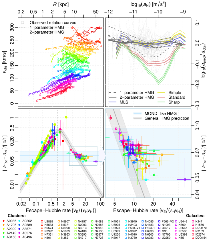
Figure 2: Galaxy rotation curves (McGaugh et al., 2007, squares,) compared with cluster RAR (Li et al., 2023, circles,). Top left: Fitting of galaxy rotation curves according to the HMG model (Monjo, 2023, Eq. C14,), where $\gamma_{0}$ is modeled by Eq. 5 with one free parameter ($\epsilon_{H}$, while $\gamma_{center}=0.48\mathrm{\pi}$; dashed lines) or two parameters ($\epsilon_{H}$, $\gamma_{center}$; continuous lines). Top right: Performance of the 1-parameter (dashed gray lines) and 2-parameter (continuous gray lines) model for the ratio of predicted ($a_{pred}$) and observed ($a_{obs}$) centripetal acceleration for the 60 galaxies (light gray lines) and comparison with MOND interpolation functions (MLS, simple, standard, and sharp functions, fitted to 153 suitable galaxies): 1-$\sigma$ confidence intervals for all functions (upper and lower lines of each color) were found as in Fig. 23 of Banik et al. (2023). Bottom left: Global fitting of the dataset according to Eqs. 2 and 5. Bottom right: Zoom in on the theoretical prediction made for galaxies fitted with Eq. 5 with $\varepsilon_{H}=21_{-11}^{+32}$. As in Fig. 1, the general model prediction for galaxies (gray band) corresponds to the parameter $\varepsilon_{H}=56_{-12}^{+22}$ as an average value of the cluster fitting, with fixed $\gamma_{center}=\mathrm{\pi}/2$ and $\gamma_{U}=\mathrm{\pi}/3$. To compare, the MOND-like model and the observational constraint of the general HMG model are shown with the shaded area representing the 90% confidence interval.

3.3 Prediction for small systems

For small gravitational systems, the escape velocity $v_{E}$ is much higher than the Hubble flux $v_{H}$, so it is expected that the cosmic effects are negligible (with $v_{E}/v_{H}\gg\varepsilon_{H}$). This is because the ratio between escape speed and Hubble flux is independent of the size of a spherical system with constant density, but smaller systems are usually much denser than larger systems. For example, according to Eq. 5, an anomaly of only $6.4_{-0.4}^{+1.0}\times 10^{-17}\;\text{m/s}^{2}$ (90% confidence level) is predicted for the Solar System at a distance of the Pluton orbit (40 AU). The predicted anomaly is even smaller for Saturn at 10 AU, which is well consistent with the null detection of anomalous effects there from Cassini radio tracking data (Hees et al., 2014; Desmond et al., 2024). For the Oort cloud, which hypothetically extends between 2 and 200 kAU, the predicted anomaly $\Delta a:=\gamma_{0}^{-1}c/t$ increases from $2.2_{-0.1}^{+0.4}\times 10^{-14}\;\text{m/s}^{2}$ to $2.3_{-0.1}^{+0.4}\times 10^{-11}\;\text{m/s}^{2}$, respectively. The last one is about 20% of the Milgrom acceleration $a_{0}\approx 1.2\times 10^{-10}\;\text{m/s}^{2}$ and could therefore be detected in the future. The most aligned finding is that shown by the work of Migaszewski (2023), who suggest that Milgromian gravity could explain the observed anomalies of extreme trans-Neptunian objects such as the Oort cloud (2–200 kAU, up to 20% of $a_{N}$). Brown & Mathur (2023) claimed that the farthest Kuiper Belt objects ($\sim 250$ AU) also present a MOND signal, but the orbit integrations performed by Vokrouhlický et al. (2024) suggest that this interpretation neglects the crucial role of the external field direction rotating as the Sun orbits the Galaxy. Therefore, these findings require further analysis to compare them with the hypothesis of a ninth planet in the trans-Neptunian region (Batygin et al., 2024). In fact, Vokrouhlický et al. (2024) exclude the possible effects of MOND on scales up to about 5–10 kAU, which is more consistent with the findings of Migaszewski (2023).

In the case of wide binaries, the typical escape speed at $r\sim 0.1$ pc is about $v_{E}=500$ m/s, while the Hubble flux is $v_{H}=r/t\sim 7\times 10^{-3}\;\text{m/s}$. Thus, the Newtonian acceleration is $a_{N}=\frac{1}{2}v_{E}^{2}/r\sim 4.1\times 10^{-11}\;\text{m/s}^{2}<a_{0}\approx 1.2\times 10^{-10}\;\text{m/s}^{2}$, which is theoretically within the classical MOND regime of Milgrom theory ($a_{N}<a_{0}$). However, the escape flux is $v_{E}/v_{H}=7.1\times 10^{4}$, and therefore we expect a very low anomaly (i.e., a large projective angle $\gamma_{sys}$). Assuming that $\gamma_{center}=\mathrm{\pi}/2$, $\gamma_{U}=\mathrm{\pi}/3$ and a global value $\varepsilon_{H}=40_{-20}^{+30}$ in Eq. 5, the projective angle $\gamma_{sys}=\mathrm{\pi}/2-2.20_{-0.35}^{+0.14}\times 10^{-4}\mathrm{\pi}$, which corresponds to a projection parameter of $\gamma_{0}^{-1}=\gamma_{sys}^{-1}\cos\gamma_{sys}=4.4^{+0.7}_{-0.3}\times 10^{-4}$, so the acceleration anomaly would be $\Delta a:=a_{Tot}-a_{N}=\gamma_{0}^{-1}c/t=3.1^{+0.4}_{-0.2}\times 10^{-13}\;\text{m/s}^{2}$ (90% interval). The prediction corresponds to $2.8\times 10^{-13}\;\text{m/s}^{2}<\Delta a<4.3\times 10^{-13}\;\text{m/s}^{2}$ at the 95% confidence level.

Therefore, in any case, the acceleration anomalies expected for rapid-escape systems are less than 1% of the original Milgrom constant $a_{0}\approx 1.2\times 10^{-10}\;\text{m/s}^{2}$. This result is consistent with recent comparisons between standard gravity and MOND with data from Gaia wide-binary systems (Pittordis & Sutherland, 2019, 2023; Banik et al., 2023). However, some authors dispute these results by using different data selection criteria (see, for instance, Hernandez, 2023; Hernandez et al., 2023; Chae, 2023, 2024a, 2024b).

4 Concluding remarks

Acceleration is not a geometrical invariant, but depends on the reference system or framework considered. The hyperconical model showed that it is possible to derive local-scale general relativity (that is, HMG) to model gravitational systems with anomalous acceleration similar to that attributed to dark matter or dark energy (Monjo & Campoamor-Stursberg, 2023; Monjo, 2023).Other MOND-based relativistic theories also obtained good performance when modeling galaxy rotation curves with a single global parameter based on acceleration. However, parameters other than acceleration are required, given that the classical MOND-based RAR does not extend to clusters and that gravity is mostly Newtonian on scales smaller than about 10 kAU with high precision, even at low acceleration.

This Letter presented a generalized applicability of the HMG model for a wide range of acceleration anomalies in gravitational systems. Good agreement was obtained with the data collected from 10 galaxy clusters and 60 high-quality galaxy rotation curves. The technique developed for the perturbed metric follows the geometric definition of the sinus of a characteristic angle $\gamma_{sys}$ as a function of the escape speed ($v_{E}$) and the Hubble flux ($\epsilon_{H}v_{H}$), that is, $\sin\gamma_{sys}^{2}-\sin^{2}\gamma_{U}\approx\beta^{2}(r)\big{|}v_{E}^{2}-\epsilon^{2}_{H}v_{H}^{2}(r)\big{|}$ for $\gamma_{U}=\mathrm{\pi}/3$. The function $\beta(r)$ does not depend on the speeds, but can be avoided by setting two parameters in $\gamma_{sys}=\gamma_{sys}(\gamma_{center},\varepsilon_{H})$: a central projective angle $0.47\mathrm{\pi}\lesssim\gamma_{center}\lesssim 0.50\mathrm{\pi}$ and a relative density $\varepsilon_{H}\geq 1$.

From the fitting of the general model of $\gamma_{sys}$ (Eq. 5) to the cluster RAR data, an anomaly between $0.05\,c/t$ and $0.40\,c/t$ is predicted for the galaxy rotation dynamics, which is statistically compatible with the observations of $0.07_{-0.02}^{+0.03}c/t$. As for any modified gravity, the challenge was to derive a tight RAR compatible with observations with few free parameters. Classical MOND only has a global free parameter $a_{0}$, but does not specify the interpolating function, so MOND actually has a high freedom to fit the observations of galactic dynamics. In contrast, the HMG model derives a unique interpolation function for rotation curves using only two parameters $(\varepsilon_{H},\gamma_{center})$ that are not totally free, since they are related to the density of matter.

For objects of the outer Solar System such as the farthest Kuiper Belt objects or the Oort cloud, anomalies between $10^{-14}\;\text{m/s}^{2}$ and $10^{-11}\;\text{m/s}^{2}$ are predicted at $1$ kAU and at $100$ kAU, respectively. Similarly, for wide binary systems, anomalies are expected within the range of $2.8\times 10^{-13}<\Delta a<4.3\times 10^{-13}\;\text{m/s}^{2}$ (95% confidence level). Such small predicted anomalies imply that local wide binaries should be Newtonian to high precision, as is within the observational limits. This work provides a chance to falsify a wide range of predictions of a relativistic MOND-like theory that has previously collected successful results in cosmology (Monjo, 2024a). In future work, we will address other open challenges, such as the modeling of cosmic structure growth and dynamics as well as the evolution of early stages of the universe.

Data Availability

In this study, no new data was created or measured.

Appendix A Perturbed vacuum Lagrangian density

This appendix summarizes the definition of the local Einstein field equations according to the hyperconical model, that is, by assuming that GR is only valid at local scales (Monjo & Campoamor-Stursberg, 2020; Monjo, 2024a). In particular, the new Lagrangian density of the Einstein-Hilbert action is obtained by extracting the background scalar curvature $R_{hyp}$ from the total curvature scalar $R\to\Delta R:=R-R_{hyp}$ as follows:

$$\mathcal{L}=\frac{1}{16\mathrm{\pi}{G}}\Delta R+\mathcal{L}_{M}\;=\;\frac{1}{16\mathrm{\pi}{G}}\left(R+\frac{6}{t^{2}}\right)-\rho_{M}\;=\;\frac{c^{2}}{16\mathrm{\pi}{G}}R-\Delta\rho\,,$$ (A1)

where ${G}$ is the Newtonian constant of gravitation, $R_{hyp}=-{6}/{t^{2}}$ is the curvature scalar of the (empty) hyperconical universe, $\mathcal{L}_{M}=-\rho_{M}$ is the Lagrangian density of classical matter, and $\Delta\rho:=\rho_{M}-\rho_{vac}$ is the density perturbation compared to the ‘vacuum energy’ $\rho_{vac}=3/(8\mathrm{\pi}{G}t^{2})$ with mass-related event radius $r_{M}:=2G\widetilde{M}:=2G\rho_{vac}\,\frac{4}{3}\mathrm{\pi}t^{3}=t$, where $\widetilde{M}$ is a ‘total mass’ linked to $\rho_{vac}$. Moreover, the squared escape velocity associated with $\rho_{vac}$ at $r$ is $v_{E}^{2}(\rho_{vac})=2{G}\rho_{vac}\,\frac{4}{3}\mathrm{\pi}r^{3}=r^{2}/t^{2}=v_{H}^{2}$. Therefore, a total density $\rho_{M}$ leads to a total (classical) squared escape velocity $v_{E}^{2}(\rho_{M})$ as follows:

$$v_{E}^{2}(\rho_{M})=2{G}\rho_{M}\,\frac{4}{3}\mathrm{\pi}r^{3}=2{G}\left(\rho_{vac}+\Delta\rho\right)\,\frac{4}{3}\mathrm{\pi}r^{3}=\frac{r^{2}}{t^{2}}+\frac{2{G}M}{r}=v_{E}^{2}(\rho_{vac})+v_{E}^{2}(\Delta\rho)\,,$$ (A2)

where we use the definition of $M:=\Delta\rho\,\frac{4}{3}\mathrm{\pi}r^{3}$. Now, let $\theta_{M}:=M/\widetilde{M}\ll 1$ be a (small) constant fraction of energy corresponding to the perturbation $\Delta\rho$, and $r_{M}:=2GM=\theta_{M}t$ be the radius of the mass-related event horizon. Thus,

$$\frac{2{G}M}{r}=\frac{\theta_{M}t}{r^{\prime}\frac{t}{t_{0}}}=\frac{\theta_{M}t_{0}}{r^{\prime}}=:\frac{2{G}M_{0}}{r^{\prime}}\,.$$ (A3)

Therefore, the quotient $M/r=M_{0}/r^{\prime}$ is as comoving as $r/t=r^{\prime}/t_{0}$.

Moreover, the background metric of the universe has a Ricci tensor with components $R_{00}^{u}=0$ and $R_{ij}^{u}=\frac{1}{3}{R}_{u}\,g_{ij}$ (Monjo, 2017; Monjo & Campoamor-Stursberg, 2020). Since $R_{hyp}=-6/t^{2}$, the Einstein field equations become locally converted to (Monjo, 2024a):

$$\begin{cases}\kappa P_{00}&=\Delta R_{00}-\frac{1}{2}\Delta Rg_{00}\;\;=\;\;R_{00}-\frac{1}{2}Rg_{00}-\frac{3}{t^{2}}g_{00}\\ \kappa P_{ij}&=\Delta R_{ij}-\frac{1}{2}\Delta Rg_{ij}\;\;=\;\;R_{ij}-\frac{1}{2}Rg_{ij}-\frac{1}{t^{2}}g_{ij}\end{cases}\,,$$ (A4)

where $\kappa=8\mathrm{\pi}{G}$ and $P_{\mu\nu}$ are the stress-energy tensor components. Notice that, for small variations in time $\Delta t=t-t_{0}\ll t_{0}:=1$, the last terms ($3/t^{2}$ and $1/t^{2}$) are equivalent to consider a ‘cosmological (almost) constant’ or dark energy with equation of state $w=-1/3$ (varying as $a^{-2}$).

Appendix B Hyperconical modified gravity (HMG)

B.1 Hyperconical universe and its projection

This appendix reviews the main features of relativistic MOND-like modified gravity derived from the hyperconical model and referred to here as HMG (Monjo, 2017, 2018; Monjo & Campoamor-Stursberg, 2020, 2023; Monjo, 2023). Let ${\pazocal{H}^{4}}$ be a (hyperconical) manifold with the following metric:

$$ds^{2}_{hyp}\approx dt^{2}\left(1-kr^{\prime 2}\right)-\frac{t^{2}}{t_{0}^{2}}\left(\frac{dr^{\prime 2}}{1-kr^{\prime 2}}+{r^{\prime}}^{2}d{\Sigma}^{2}\right)-\;\;\frac{2r^{\prime}t}{t_{0}^{2}}\frac{dr^{\prime}dt}{\sqrt{1-kr^{\prime 2}}}\,,$$ (B1)

where $k=1/t_{0}^{2}$ is the spatial curvature for the current value $t_{0}\equiv 1$ of the age $t$ of the universe, while $\frac{a}{(}t):=t/{t_{0}}$ is a scale factor, $r^{\prime}\ll t_{0}$ is the comoving , and $\Sigma$ represents the angular coordinates. Both the (Ricci) curvature scalar and the Friedmann equations derived for $k=1$ are locally equivalent to those obtained for a spatially flat ($K_{FLRW}=0$) $\Lambda$CDM model with linear expansion (Monjo & Campoamor-Stursberg, 2020). In particular, the local curvature scalar at every point ($r^{\prime}\equiv 0$) is equal to (Monjo, 2017):

$$R_{hyp}=-\frac{6}{t^{2}}=R_{FLRW}\bigg{|}_{K\,=\,0,\;a\,=\,t/t_{0}}\,,$$ (B2)

as for a three-sphere (of radius $t$). This is not accidental because, according to Monjo & Campoamor-Stursberg (2020), the local conservative condition in dynamical systems only ensures internal consistency for $k=1$.

The hyperconical metric (Eq. B1) has shift and lapse terms that produce an apparent radial inhomogeneity, which is equivalent to an acceleration. This inhomogeneity can be assimilated as an apparent acceleration by applying some ‘flattening’ or spatial projection. In particular, for small regions, a final intrinsic comoving distance $\hat{r}^{\prime}$ can be defined by an $\alpha$-distorting stereographic projection (Monjo, 2018; Monjo & Campoamor-Stursberg, 2023),

$$r^{\prime} \mapsto \hat{r}^{\prime}=\frac{r^{\prime}}{\left(1-\frac{\gamma(r^{\prime})}{\gamma_{0}}\right)^{\alpha}}\,,$$ (B3)

$$t \mapsto \hat{t}=\frac{t}{1-\frac{\gamma(r^{\prime})}{\gamma_{0}}}\,,$$ (B4)

where $\gamma=\gamma(r^{\prime}):=\sin^{-1}(r^{\prime}/t_{0})$ is the angular comoving coordinate, $\gamma_{0}^{-1}\in(0,1)$ is a projection factor, and $\alpha=1/2$ is a distortion parameter, which is fixed according to symplectic symmetries (Monjo & Campoamor-Stursberg, 2023). Locally, for empty spacetimes, it is expected that $\gamma_{0}\approx 2$; which is compatible with the fitted value of $\gamma_{0}=1.6^{+0.4}_{-0.2}$ when Type Ia SNe observations are used (Monjo & Campoamor-Stursberg, 2023). In summary, the projection factor $\gamma_{0}$ depends on a projective angle $\gamma_{sys}$ such that $\gamma_{0}=\gamma_{sys}/\cos(\gamma_{sys})\geq 1$, where $\gamma_{0}=2$ corresponds to a total empty projective angle of $\gamma_{sys}\approx\mathrm{\pi}/3$, and $\gamma_{0}=1$ is the minimum projection angle allowed by the causality relationship of the arc length $\gamma_{0}t_{0}$. Therefore, the projective angle for an empty or almost empty neighborhood is approximately $\gamma_{neigh}=(0.284\pm 0.049)\mathrm{\pi}\lesssim\mathrm{\pi}/3=:\gamma_{U}$.

B.2 Perturbation by gravitationally bound systems

In the case of an (unperturbed) homogeneous universe, the linear expansion of ${\pazocal{H}^{4}}$ can be expressed in terms of the vacuum energy density $\rho_{vac}(t)=3/(8\mathrm{\pi}{G}t^{2})$, where ${G}$ is the Newtonian gravitational constant, and thus $\rho_{vac}(t_{0})=\rho_{crit}$. That is, one can define an inactive (vacuum) mass or energy $\mathcal{M}(r)=\rho_{vac}\frac{4}{3}\mathrm{\pi}r^{3}$ for a distance equal to $r$ with respect to the reference frame origin. Using the relationship between the original coordinates $(dt,dr,r\,d{\Sigma})$ and the comoving ones $(dt,\frac{a}{(}t)\,dr^{\prime},\frac{a}{(}t)r^{\prime}d{\Sigma})$, the spatial dependence of the metric is now

$$\frac{{r^{\prime}}^{2}}{t_{0}^{2}}=\frac{{r}^{2}}{t^{2}}=\frac{2{G}\rho_{vac}\frac{4}{3}\mathrm{\pi}r^{3}}{r}=\frac{2{G}\mathcal{M}(r)}{r}=v_{H}^{2}(r)\,,$$ (B5)

where $v_{H}(r):=r/t$ is the Hubble speed, which coincides with the escape speed of the empty spacetime with vacuum density $\rho_{vac}$.

Definition B.1 (Mass of perturbation)

A perturbation of the vacuum density $\rho_{vac}\to\rho_{M}(r):=\rho_{vac}+\Delta\rho$, with an effective density $\Delta\rho$ at $r>0$, leads to a system mass $M_{sys}:=\frac{4}{3}\mathrm{\pi}r^{3}\Delta\rho$ that is likewise obtained by perturbing the curvature term,

$$\frac{r^{2}}{t^{2}}\to\frac{r^{2}}{t_{sys}(r)^{2}}:=\frac{r^{2}}{t^{2}}+\frac{2{G}M_{sys}}{r}=v_{H}^{2}(r)+v_{E}^{2}(r)\,,$$ (B6)

with a radius of curvature $t_{sys}(r)\in(2{G}M_{sys},t]$, where $v_{E}(r):=\sqrt{2{G}M_{sys}/r}$ is the classical escape speed (Eq. A2).

An approximation to the Schwarzschild solution can be obtained in a flat five-dimensional ambient space from the hyperconical metric. For example, let $(t,\vec{r},u):=(t,x,y,z,u)\in\mathbb{R}_{\eta}^{1,4}$ be Cartesian coordinates, including an extra spatial dimension $u$ in the five-dimensional Minkowski plane. As used in hyperconical embedding, $u:=t\cos\gamma-t$ is chosen to mix space and time. Now, it includes a gravity field with system mass $M_{sys}$ integrated over a distance $\hat{r}$ such that $\sin^{2}\gamma:=\frac{r^{2}}{t^{2}}\mapsto\frac{\hat{r}^{2}}{t^{2}}+\frac{2{G}{M_{sys}}}{\hat{r}}$. Notice that $r$ is a coordinate related to the position considered, in contrast to the observed radial distance $\hat{r}$ or its comoving distance $\hat{r}^{\prime}:=(t_{0}/t)\hat{r}$. With this, first-order components $\hat{g}_{\mu\nu}$ of the metric perturbed by the mass are:

$$\hat{g}_{tt} = 2\cos\gamma-1\;\;\approx\;\;1-\frac{{\hat{r}}^{2}}{t^{2}}-\frac{2{G}M_{sys}}{{\hat{r}}}\,,$$

$$\hat{g}_{r^{\prime}r^{\prime}} = -\frac{t^{2}}{t_{0}^{2}}\frac{1}{\cos^{2}\gamma}\;=\;-\frac{t^{2}}{t_{0}^{2}}\left(1-\frac{{\hat{r}}^{2}}{t^{2}}-\frac{\mathrm{2G}{M_{sys}}}{{\hat{r}}}\right)^{-1}\approx-\frac{t^{2}}{t_{0}^{2}}\left(1+\frac{{\hat{r}}^{2}}{t^{2}}+\frac{\mathrm{2G}{M_{sys}}}{{\hat{r}}}\right)\,,$$

$$\hat{g}_{r^{\prime}t} = \frac{t}{t_{0}}\tan\gamma\;\;=\;\;\frac{t}{t_{0}}\frac{\hat{r}}{t}\left(1-\frac{{\hat{r}}^{2}}{t^{2}}-\frac{2{G}{M_{sys}}}{{\hat{r}}}\right)^{-1/2}\;\approx\;\frac{t}{t_{0}}\frac{\hat{r}}{t}+O\left(\frac{{\hat{r}}^{3}}{2t^{3}}\right)\,,$$

$$\hat{g}_{\theta\theta} = -\frac{t^{2}}{t_{0}^{2}}{\hat{r}}^{\prime 2}\,,$$

$$\hat{g}_{\varphi\varphi} = -\frac{t^{2}}{t_{0}^{2}}{\hat{r}}^{\prime 2}\sin^{2}\theta\,,$$

where the hyperconical model is recovered taking $M_{sys}=0$. Therefore, assuming linearized perturbations of the metric $\hat{g}_{\mu\nu}=\hat{g}_{\mu\nu}^{back}+\hat{h}_{\mu\nu}$ with $\hat{g}_{\mu\nu}^{back}:=\hat{g}_{\mu\nu}|_{M_{sys}=\,0}$, we can find a local approach to the Schwarzschild metric perturbation $h|_{Schw}$ as follows (Monjo, 2023):

$${\hat{g}}_{Schw} :\approx \left[\eta_{\mu\nu}+\left(\hat{g}_{\mu\nu}-\hat{g}_{\mu\nu}^{back}\right)\right]dx^{\mu}dx^{\nu}\approx$$

$$\approx \left(1-\frac{2{G}{M_{sys}}}{\hat{r}}\right)d{\hat{t}}^{2}-\frac{t^{2}}{t_{0}^{2}}\left[\left(1+\frac{2{G}{M_{sys}}}{\hat{r}}\right)d{{\hat{r}}^{\prime 2}}+{{\hat{r}}^{\prime 2}}d{\Sigma}^{2}\right]\,+\text{shift}\,,$$

which is also obtained for $\hat{g}_{\mu\nu}$ when $\hat{r}/t\ll 1$, that is $\lim_{(\hat{r}/t_{0})\to 0}[\hat{g}_{\mu\nu}]\approx{\hat{g}}_{Schw}$. The shift term is neglected in comparison to the other terms, especially for geodesics. Our result is aligned to the Schwarzschild-like metric obtained by Mitra (2014) for FLRW metrics, specifically for the case of $K=0$.

In summary, the first-order approach of the 5-dimensionally embedded (4-dimensional) hyperconical metric (Eq. LABEL:eq:Schwarzschild_g) differs from the Schwarzschild vacuum solution by the scale factor $t^{2}/t_{0}^{2}$ and by a negligible shift term. Therefore, the classical Newtonian limit of GR is also recovered in the hyperconical model, because the largest contribution to gravitational dynamics is given by the temporal component of the metric perturbation $h_{tt}$. That is, the Schwarzschild geodesics are linearized by

$$\frac{d^{2}x^{\mu}}{d\tau^{2}}\approx\frac{1}{2}\eta^{\mu\nu}\frac{\partial}{\partial x^{\nu}}h_{tt}\left(\frac{dt}{d\tau}\right)^{2}\;,$$ (B8)

where $\hat{h}_{tt}\approx-2{G}M_{sys}/{\hat{r}}$.

Appendix C Modeling radial acceleration

C.1 Projective angles of the gravitational system

The last appendix derived a general expression for the anomalous RAR expected for any gravitational system according to the projective angles (which depend on the quotient between escape speed and Hubble flux) under the hyperconical universe framework.

From the analysis of perturbations (Eq. B6), it is expected that any gravitational system (Eq. LABEL:eq:Schwarzschild_g) results in a characteristic scale $r_{cs}(M_{sys}(r)):=t_{sys}(r)\sin\gamma_{sys}(r)$ given by a projective angle $\gamma_{sys}\in[\mathrm{\pi}/3,\mathrm{\pi}/2)$ that slightly depends on the radial distance $r$ and on the mass $M_{sys}$. Unlike gravitational lensing, a non-null cosmic projection $\gamma_{0}^{-1}=\gamma_{sys}^{-1}\cos\gamma_{sys}>0$ is expected for non-concentrated gravitational systems. In particular, we assume that the maximum projective angle ($\gamma_{sys}=\gamma_{center}:=\mathrm{\pi}/2$, minimum cosmic projection) is produced by small, dense, and homogeneous gravitational systems, while the minimum angle ($\gamma_{sys}=\gamma_{U}:=\mathrm{\pi}/3$, maximum cosmic projection) corresponds to large systems extended towards an (almost) empty universe (Fig. C.1). Since $t_{sys}^{2}(r)\in(4{G}^{2}M_{sys}^{2},t^{2}]$ and $r_{cs}^{2}(M)\in(4{G}^{2}M_{sys}^{2},\frac{3}{4}t^{2}]$, the characteristic scale $\,r_{cs}^{2}(M_{sys})$ increases from $r_{cs}^{2}(M_{sys})=t_{sys}^{2}(r)=4{G}^{2}M_{sys}^{2}\ll t^{2}$ up to $r_{cs}^{2}(M_{sys})=\frac{3}{4}t_{sys}^{2}(r)=\frac{3}{4}t^{2}=t^{2}\sin^{2}\gamma_{U}$; that is, $\sin\gamma_{sys}^{2}(r)\in[\frac{3}{4},1]$.

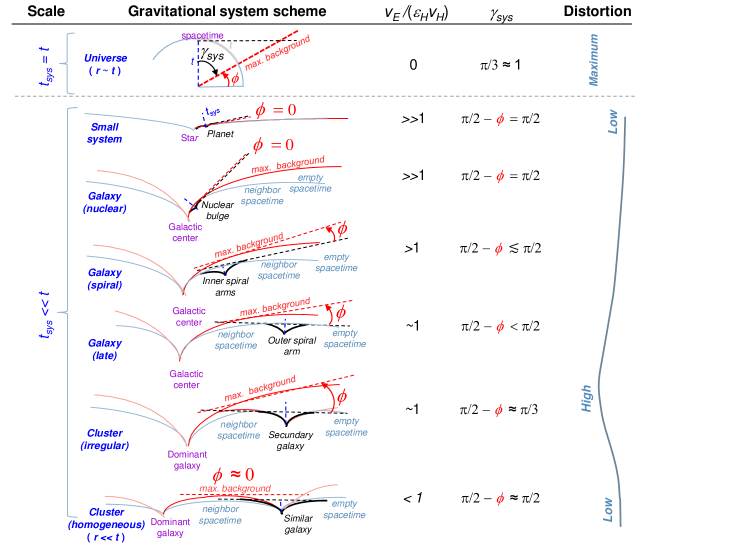
Figure C.1: Conceptual model of the projective angle $\gamma_{sys}$ as a function of the relative geometry (escape speed $v_{E}$ over the Hubble flux $\varepsilon_{H}v_{H}$), for each gravitational system (black curves), with respect to the maximum background spacetime (red curves). To simplify the scheme, the projection factor $\gamma_{0}^{-1}:=\gamma_{sys}^{-1}\cos\gamma_{sys}$ is graphically represented by an auxiliary angle $\phi$ defined as the arc between the hyperplane of the gravitational system (dashed black line) and the maximum background hyperplane (dashed red line) curved by the dominant system (purple), such that $\gamma_{sys}=\mathrm{\pi}/2-\phi$. The distance scale $r$ is represented by $t_{sys}$ (Eq. B6). In addition to the cosmic scale, six gravitational systems are considered: i) a small system (e.g. Solar System); ii) an early-type galaxy with a dominant nuclear bulge; iii) a typical spiral galaxy; iv) a late-type spiral galaxy; v) an irregular cluster; and vi) a homogeneous cluster. The dominant objects (purple terms) are the star for a small system, the galactic center for galaxies, and the brightest galaxy for a given cluster.

The relation of $\gamma_{sys}$ with respect to the gravitational mass and the scale of speeds can be estimated from the following properties. According to Eq. B6, a gravitational system perturbs the cosmological geometry with (squared) escape speed of $v_{E}^{2}(r):=\frac{2{G}M_{sys}}{r}$ higher than the Hubble expansion speed $v_{H}^{2}(r):=\frac{r^{2}}{t^{2}}$, so the projective angle $\gamma_{sys}$ is given by:

$$\sin^{2}\gamma_{sys}(r) = \frac{r_{cs}^{2}(M_{sys})}{t_{sys}^{2}(r)}=\frac{r_{cs}^{2}(M_{sys})}{t^{2}}+\frac{2r_{cs}^{2}(M_{sys})\,{G}M_{sys}}{r^{3}}=$$ (C1)

$$\approx \;\;\sin^{2}\gamma_{neigh}+\beta^{2}(r)v_{E}^{2}\;\sim\;\sin^{2}\gamma_{U}-\beta^{2}(r)\epsilon^{2}_{H}v_{H}^{2}(r)+\beta^{2}(r)v_{E}^{2}\,,{}$$

where $\beta^{2}(r):=r_{cs}^{2}/r^{2}\gg 1$ is an auxiliary function, $\gamma_{neigh}:=\sin^{-1}(r_{cs}/t)\in(0,\gamma_{U})$ is a characteristic neighbor angle, and $\epsilon^{2}_{H}:=\sin^{2}\gamma_{U}/\sin^{2}\gamma_{neigh}-5/6\propto t^{2}/r_{cs}^{2}\propto\rho/\rho_{vac}$ is a relative density of the neighborhood matter ($\rho$) with respect to the vacuum density ($\rho_{vac}$; Eq. A2). So, roughly speaking, it is $\sin^{2}\gamma_{neigh}(r)\sim\frac{5}{6}\sin^{2}\gamma_{neigh}(r)=\sin^{2}\gamma_{U}-\epsilon^{2}_{H}r_{cs}^{2}/t^{2}$. On the other hand, the center of the gravitational system presents a higher density, thus the cosmic projection should be minimum due to the maximum projective angle $\gamma_{center}\approx\mathrm{\pi}/2$, that is,

$$1\approx\sin^{2}\gamma_{center}\approx\frac{r_{cs}^{2}(M_{sys})}{t_{sys}^{2}(r)}+2\epsilon_{H}^{2}\frac{r_{cs}^{2}(M_{sys})}{t^{2}}\sim\sin^{2}\gamma_{U}+\beta^{2}(r)\epsilon^{2}_{H}v_{H}^{2}+\beta^{2}(r)v_{E}^{2}\,.$$ (C2)

Notice that, for the limit when $\gamma_{neigh}\approx\gamma_{U}$, it is required that $\epsilon^{2}_{H}\approx\frac{1}{6}$ and $v_{E}\approx 0$. The dependency of $\gamma_{sys}$ on the auxiliary function $\beta(r)$ can be removed by taking the quotient of $\sin^{2}\gamma_{sys}(r)-\sin^{2}\gamma_{U}$ (Eq. C1) over $\sin^{2}\gamma_{center}-\sin^{2}\gamma_{U}$ (Eq. C1). Therefore, it is expected that the projective angle $\gamma_{sys}$ of every gravitational system presents a general relation similar to

$$\frac{\sin^{2}\gamma_{sys}(r)-\sin^{2}\gamma_{U}}{\sin^{2}\gamma_{center}-\sin^{2}\gamma_{U}}\sim\bigg{|}\frac{v_{E}^{2}(r)-\epsilon^{2}_{H}v_{H}^{2}(r)}{v_{E}^{2}(r)+\epsilon^{2}_{H}v_{H}^{2}(r)}\bigg{|}\,,$$ (C3)

with two free parameters, $\epsilon_{H}\geq\frac{1}{6}$ and $\gamma_{center}\approx\frac{1}{2}\mathrm{\pi}$. For example, for galaxies and small gravitational systems, the escape speed $v_{E}^{2}$ is strongly related to the Kepler orbital speed $v_{K}^{2}\approx v_{E}^{2}/2\sim v_{E}^{2}$, and the projective angle $\gamma_{sys}(r)\equiv\gamma_{galaxy}(r)$ can be estimated by the following galactic relation (Monjo, 2023):

$$\frac{\sin^{2}\gamma_{galaxy}(r)-\sin^{2}\gamma_{neigh}}{\sin^{2}\gamma_{center}-\sin^{2}\gamma_{U}}\sim\frac{v_{E}^{2}(r)}{\epsilon^{2}_{H}v_{H}^{2}(r)+v_{E}^{2}(r)}\,,$$ (C4)

with $\gamma_{neigh}\sim\gamma_{U}\approx\mathrm{\pi}/3$ and one free parameter, which is $\epsilon^{2}_{H}\gtrsim 1$ if $\gamma_{center}=\mathrm{\pi}/2$ is fixed, or $\gamma_{center}\lesssim\mathrm{\pi}/2$ if $\epsilon_{H}=1$ is fixed. Thus, two limiting cases are $\sin\gamma_{sys}\approx 1\,\Rightarrow\,\gamma_{sys}\approx\mathrm{\pi}/2$ when orbital speed is $v_{K}(r)\sim v_{E}(r)\gg\varepsilon_{H}v_{H}(r)$, while $\sin\gamma_{sys}\approx\frac{\sqrt{3}}{2}\,\Rightarrow\,\gamma_{sys}\approx\mathrm{\pi}/3$ when orbital speed is $v_{K}(r)\sim v_{E}(r)\ll\varepsilon_{H}v_{H}(r)$, which is the lower limit of the neighborhood projective angle ($\gamma_{neigh}$).

On the other hand, radial accelerations (without regular orbits) of large-scale objects such as galaxy clusters are expected to present opposite behavior with respect to Eq. C4, since the gravitational center is not a galactic black hole but is close to a dominant galaxy (Shi et al., 2023; De Propris et al., 2020, the brightest cluster galaxies, BCGs;), and the neighborhood now corresponds to the large-scale environment of the clusters themselves. Therefore, the projective angle $\gamma_{cluster}$ of the largest structures is approximated by the following cluster relation:

$$\frac{\sin^{2}\gamma_{galaxy}-\sin^{2}\gamma_{cluster}(r)}{\sin^{2}\gamma_{galaxy}-\sin^{2}\gamma_{U}}\sim\frac{v_{E}^{2}(r)}{\epsilon^{2}_{H}v_{H}^{2}(r)+v_{E}^{2}(r)}\,,$$ (C5)

where $v_{E}^{2}(r)$ is the escape speed of the clusters, $\gamma_{center}\sim\gamma_{galaxy}\lesssim\mathrm{\pi}/2$ is the averaged projective angle for galaxies and, now, we expect that the projective angle for clusters is a variable $\gamma_{cluster}(r)\in[\mathrm{\pi}/3,\mathrm{\pi}/2)$, but close to the neighborhood value $\gamma_{neigh}\sim\gamma_{U}=\mathrm{\pi}/3$.

However, a perfectly homogeneous distribution of low-density galaxies in a cluster will lead to a balance between the different galaxies that form it, so the cluster radial acceleration will be approximately zero ($v_{E}\sim 0$) and anomalies are not expected, thus the projective angle will be $\gamma_{cluster}\approx\mathrm{\pi}/2$ for both Eq. C3 and Eq. C5; that is, no significant geometrical differences are expected between the external and internal parts of the cluster (see the last case of Fig. C.1). Conversely, for irregular clusters ($v_{E}\sim\epsilon_{H}v_{H}$ with $\epsilon_{H}\gg 1$ in Eq. C3 or $v_{E}^{2}\gtrsim\epsilon^{2}_{H}v_{H}^{2}(r)$ in Eq. C5), the radial acceleration will be very similar to the cosmic expansion (with angle $\gamma_{cluster}=\gamma_{U}=\mathrm{\pi}/3$). Notice that, for very inhomogeneous systems ($v_{E}\gg\epsilon_{H}v_{H}$), Eq. C3 recovers the behavior of high-density galaxies (Eq. C4) with $\gamma_{cluster}(r)=\gamma_{galaxy}(r)$. Moreover, for $v_{E}\in(0,\;\epsilon_{H}v_{H})$, Eq. C3 behaves in a similar way as in Eq. C5 as expected.

C.2 Cosmological projection of the Schwarzschild metric

Henceforth, the constant of light speed $c\equiv 1$ will not be omitted from the equations so we can compare with real observations later. Let $\lambda$ be the scaling factor of an $\alpha$-distorting stereographic projection (Eq. B3) of the coordinates $(r^{\prime},u)=(ct\sin\gamma,\;ct\cos\gamma)\in\mathbb{R}^{2}$, used to simplify the spatial coordinates $({\vec{r}}^{\prime},u)\in\mathbb{R}^{4}$ due to angular symmetry. For nonempty matter densities, we contend that $\gamma_{sys}$ depends on the escape speed of the gravity system considered. However, the first-order projection can be performed by assuming that the dependence on distances is weak (i.e., with $\gamma_{0}^{-1}=\gamma_{sys}^{-1}\cos\gamma_{sys}$ being approximately constant for each case). Thus, the stereographic projection is given by the scale factor $\lambda$ such as (Monjo & Campoamor-Stursberg, 2023; Monjo, 2023, see for instance):

$$\lambda=\frac{1}{1-\frac{\gamma}{\gamma_{0}}}\approx{1+\frac{r^{\prime}}{\gamma_{0}t_{0}c}}\,,$$ (C6)

where $\gamma=\sin^{-1}[r^{\prime}/(t_{0}c)]\approx r^{\prime}/(t_{0}c)$ is the angular position of the comoving distance $r^{\prime}=(t_{0}/t)\,r$. Therefore, the projected coordinates are

$$\begin{cases}\hat{r}^{\prime}=\lambda^{\alpha}r^{\prime}\approx\left({1+\frac{\alpha r^{\prime}}{\gamma_{0}t_{0}c}}\right)r\,,\\ \hat{t}=\lambda t\approx\left(1+\frac{r^{\prime}}{\gamma_{0}t_{0}c}\right)t\,,\end{cases}$$ (C7)

At a local scale, the value of $\alpha=1/2$ is required to guarantee consistency in dynamical systems (Monjo & Campoamor-Stursberg, 2023), but the parameter $\alpha$ is not essential in this work, since only the temporal coordinate is used in our approach below.

Applying this projection to the perturbed metric (Eq. LABEL:eq:Schwarzschild_g) and obtaining the corresponding geodesics, it is easy to find a first-order approach of the cosmic contribution to modify the Newtonian dynamics in the classical limit, as shown below (Sec. C.3).

C.3 First-order perturbed geodesics

Assuming that the projection factor $\gamma_{0}^{-1}=\gamma_{sys}^{-1}\cos\gamma_{sys}$ is approximately constant, the quadratic form of the projected time coordinate (Eq. C7) is as follows:

$$d\hat{t}^{2}\approx\left(1+\frac{2r^{\prime}}{\gamma_{0}t_{0}c}+\frac{2t\dot{r}^{\prime}}{\gamma_{0}t_{0}c}\right)dt^{2}\;\;+\;\;\text{higher-order terms}\,.$$ (C8)

By using these prescriptions, our Schwarzschild metric (Eq. LABEL:eq:Schwarzschild_g) is expressed in projected coordinates $(\hat{t},\hat{r}^{\prime})$ or in terms of the original ones $(t,r^{\prime})$; that is, ${\hat{g}}_{Schw}=\hat{g}_{\mu\nu}d\hat{x}^{\mu}d\hat{x}^{\nu}={g}_{\mu\nu}d{x}^{\mu}d{x}^{\nu}$, with

$${\hat{g}}_{Schw} \approx \left(1-\frac{2{G}M_{sys}}{c^{2}\hat{r}}\right)c^{2}d\hat{t}^{2}-\frac{\hat{t}^{2}}{t_{0}^{2}}\,{\hat{r}^{\prime 2}}d{\Sigma}^{2}\;\;\approx\;\;g_{tt}c^{2}dt^{2}+g_{ii}(dx^{i})^{2}\,,$$

and finally, it is locally expanded up to first-order perturbations in terms of $\gamma_{0}$. Notice that, according to Eq. LABEL:eq:Schwarzschild_g, the background terms $r^{\prime 2}/t_{0}^{2}$ do not produce gravitational effects and thus they can be neglected. Here, one identifies a projected perturbation $h_{tt}$ of the temporal component of the metric, $g_{tt}=\eta_{tt}+h_{tt}=1+h_{tt}$, with $\eta_{\mu\nu}=\eta^{\mu\nu}=\mathrm{diag}(1,-1,-1,-1)$. Thus, if $M_{sys}$ is assumed to be mostly concentrated in the central region of the gravitional system, the first-order perturbation of the temporal component of the metric is

$$h_{tt}\approx-\frac{2{G}M_{sys}}{rc^{2}}\left({1-\frac{\alpha r}{\gamma_{0}tc}}\right)+\frac{2}{\gamma_{0}c}\left(\frac{r}{t}+\frac{t}{t_{0}}{\dot{r}^{\prime}}\right)\,,$$ (C9)

where the spatial projection $\hat{r}\approx(1+\alpha r/(\gamma_{0}ct))\,r$ is considered (from Eq. C7), and the relation between comoving distance $r^{\prime}$ and spatial coordinate $r$ is also used ($r^{\prime}/t_{0}=r/t$).

Under the Newtonian limit of GR, the largest contribution to gravity dynamics is given by the temporal component of the metric perturbation $h_{tt}$. That is, Schwarzschild geodesics (Eq. B8) produce both time-like and space-like acceleration components from the metric perturbation $h_{tt}$,

$$\frac{d^{2}\hat{s}}{c^{2}dt^{2}}\approx\frac{1}{2}\frac{\partial}{\partial x^{0}}h_{tt}\,e_{t}\;-\;\frac{1}{2}\frac{\partial}{\partial x^{i}}h_{tt}\,e_{i}=:a^{t}e_{t}+a^{i}e_{i}\,,$$ (C10)

where the four-position $\hat{s}:=(c\Delta t,x^{i})=c\Delta t\,e_{t}\,+\,x^{i}\,e_{i}=:c\Delta\mathbf{t}+\mathbf{x}\in\mathbf{R}^{1,3}$ is assumed, with canonical basis $\{e_{t},e_{1},e_{2},e_{3}\}$ and dual basis $\{e^{t},e^{1},e^{2},e^{3}\}$. For a freely falling particle with central-mass reference coordinates $\mathbf{x}=x^{i}e_{i}=(r,0,0)=\mathbf{r}\in\mathbb{R}^{3}$, it experiences an acceleration of about

$$\frac{d^{2}\hat{s}}{dt^{2}}=a^{t}e_{t}+a^{r}e_{r}\approx\;\left(\frac{\dot{r}^{\prime}}{t_{0}}-\frac{r+\frac{1}{2}\alpha r_{M}}{\gamma_{0}t^{2}}\right)e_{t}\;-\;\left(\frac{{G}M_{sys}}{r^{2}}+\frac{c}{\gamma_{0}t}\right)\frac{\mathbf{r}}{r}\;\approx\;a_{N}-\frac{c}{\gamma_{0}t}\frac{\mathbf{r}}{r}-\frac{r}{\gamma_{0}t^{2}}e_{t}\,,$$ (C11)

where $r_{M}:=2{G}M_{sys}/c^{2}\ll r$ is the Schwarzschild radius, which is neglected compared to the spatial position $r$. That is, an acceleration anomaly is obtained mainly in the spatial direction, about $|\mathbf{a}-a_{N}|\approx\gamma_{0}^{-1}c/t$ for $\mathbf{a}:=a^{r}e_{r}$. However, the total acceleration also has a time-like component, that is, in the direction $e_{t}$. In particular, for a circular orbit with radius $r$, and taking into account the non-zero temporal contribution to the acceleration in the hyperconical universe with radius $ct$ (Monjo, 2023), the total centrifugal acceleration is

$$\frac{v^{2}}{c^{2}}{e_{s}}=-\left(cte_{t}e^{t}+x^{i}e_{i}e^{i}\right)\frac{d^{2}{\hat{s}}}{c^{2}dt^{2}}\approx\,ct\left(\frac{r}{\gamma_{0}c^{2}t^{2}}\right)\,e_{t}\;+\;\left(\frac{{G}M_{sys}}{c^{2}r^{2}}+\frac{1}{\gamma_{0}ct}\right)\frac{x^{i}x_{i}}{r}\,e_{i}\;,$$ (C12)

where $e_{s}$ is an effective space-like direction ($||e_{s}||^{2}=e_{s}e^{s}=-1$), while the absolute value of the velocity is given by

$$\frac{v^{4}}{c^{4}}=-\bigg{|}\bigg{|}\frac{v^{2}}{c^{2}}{e_{s}}\bigg{|}\bigg{|}^{2}\approx\left(\frac{{G}M_{sys}}{rc^{2}}\right)^{2}+\frac{2{G}M_{sys}}{\gamma_{0}tc^{3}}\Longrightarrow\begin{cases}v\approx\sqrt{\frac{{G}M_{sys}}{r}}\;\;\hskip 28.45274pt\mathrm{if}\;\frac{{G}M_{sys}}{r^{2}}>>\frac{2c}{\gamma_{0}t}=:a_{\gamma 0}\\ v\approx\sqrt[4]{\frac{2{G}M_{sys}c}{\gamma_{0}t}}\;\;\hskip 19.91692pt\mathrm{if}\;\frac{{G}M_{sys}}{r^{2}}<<\frac{2c}{\gamma_{0}t}=a_{\gamma 0}\end{cases}\;,$$ (C13)

which satisfies two well-known limits of Newton’s dynamics and Milgrom’s (Eq. C13 right), where $a_{0}$ is the Milogrom’s acceleration parameter and $M_{sys}=M_{sys}(r)$ is the total mass within the central sphere of radius $r$. Finally, the velocity curve $v=v(r)$ can be reworded in terms of the Kepler speed $v_{K}:=\sqrt{{G}M_{sys}(r)/r}$. Therefore, the predicted mass-discrepancy acceleration relation for rotation curves is

$$\left(\frac{v}{v_{K}}\right)^{2}\approx\sqrt{1+\frac{1}{|a_{N}|}\frac{2c}{\gamma_{0}t}}\;\;\Longrightarrow\;\;\frac{a_{C}}{a_{N}}\approx\sqrt{1+\frac{1}{|a_{N}|}\frac{2c}{\gamma_{0}t}}\,,$$ (C14)

where $a_{C}=v^{2}/r$ is the total radial acceleration and $a_{N}={G}M_{sys}/r^{2}$ is the Newtonian acceleration. However, the absence of rotation in galaxy clusters leads to a radial acceleration similar to Eq. C11. In any case, the projection factor $\gamma_{0}^{-1}=\gamma_{sys}^{-1}\cos\gamma_{sys}$ depends on the projective angle $\gamma_{sys}$, which can be estimated from the galaxy cluster approach (Eq. C5) or from the general model (Eq. C3), respectively, as follows:

$$\sin^{2}\gamma_{cluster}(r)\;\;\; \approx \;\;\;\sin^{2}\gamma_{galaxy}-\left({\sin^{2}\gamma_{galaxy}-\sin^{2}\gamma_{U}}\right)\frac{v_{E}^{2}(r)}{\varepsilon^{2}_{H}v_{H}^{2}(r)+v_{E}^{2}(r)}\,,\hskip 28.45274pt{}$$ (C15)

$$\sin^{2}\gamma_{cluster}(r)\;\;\; \approx \;\;\;\sin^{2}\gamma_{U}+\left({\sin^{2}\gamma_{center}-\sin^{2}\gamma_{U}}\right)\bigg{|}\frac{v_{E}^{2}(r)-\epsilon^{2}_{H}v_{H}^{2}(r)}{v_{E}^{2}(r)+\epsilon^{2}_{H}v_{H}^{2}(r)}\bigg{|}\,.{}$$ (C16)

where $\gamma_{center}$ can be fixed to $\gamma_{center}=\mathrm{\pi}/2$ to test the 1-parameter ($\epsilon_{H}$) general model of Eq. C16, while this study assumes that $\{\epsilon_{H},\gamma_{galaxy}\}$ are free in our 2-parameter model for clusters (Eq. C16). Finally, the empty projective angle is usually set as $\gamma_{U}=\mathrm{\pi}/3$ (Monjo & Campoamor-Stursberg, 2023), which produces a projection factor of $\gamma_{U}^{-1}\cos\gamma_{U}\approx\frac{1}{2}$.

C.4 Individual fitting

Observed data on the RAR of 10 clusters ($0.0328<z<0.0899$) were collected from the study performed by Li et al. (2023). Individually, fitting of Eq. C15 for the anomaly between the total spatial acceleration and Newtonian acceleration (Eq. C11) leads to a square root of the relative density of about $\varepsilon_{H}=38^{+29}_{-11}$ (90% confidence level, Fig. C.2). All these results are obtained by fixing the constants $\gamma_{U}=\mathrm{\pi}/3$ and $\gamma_{center}=\mathrm{\pi}/2$. The general model (Eq. C16), with only one free parameter ($\varepsilon_{H}$), gave good results for eight of the ten clusters, showing difficulties in fitting the more available data from the A2029 and A2142 clusters (Table 1). If two parameters are considered ($\varepsilon_{H}$, $\gamma_{center}$), the results considerably improve except for the A2029 cluster, which requires changing $\gamma_{U}^{-1}\cos\gamma_{U}\to 1$ to be compatibly fitted to the observations.

The same 2-parameter ($\varepsilon_{H}$, $\gamma_{center}$) general model (Eq. C16 with $\gamma_{U}=\mathrm{\pi}/3$) was also applied to the 60 high-quality galaxy rotation curves, obtaining an acceptable result for all of them. The case of 1 parameter ($\varepsilon_{H}$ free when $\gamma_{center}=0.48\mathrm{\pi}$ is set) showed a slightly larger chi-square statistic and $p$-value, but these are also acceptable for all of them. Moreover, an empirical relationship is found between the single parameter $\epsilon_{H}$ and the square root of a relative density, which defines an identity $\rho(r_{typ})/\rho_{vac}\cong 1$ in units of vacuum density $\rho_{vac}:=3/(8\mathrm{\pi}{G}t^{2})$ for an observed density $\rho(r_{typ})$ that is defined at a typical neighborhood distance of approximately four times the maximum radius ($r_{typ}\approx 4\times r_{max}$, fitted at $R=0.85$, $p$-value $<0.0001$, Fig. C.3 left) for each galaxy rotation curve, and equal to the minimum radius ($r_{typ}\approx r_{min}$) for the data of each cluster. This typical distance corresponds to $r_{typ}\approx 50-200\,$kpc.

Finally, when the 2-parameter HMG model is considered for galaxies, an additional relationship is found between $\epsilon_{H}$ and $\gamma_{center}$:

$$\cos(\gamma_{center})=\cos\left(0.4610^{+0.0013}_{-0.0014}\mathrm{\pi}\right)-(0.020\pm 0.002)\ln(\varepsilon_{H})$$ (C17)

for $1\leq\varepsilon_{H}<400$, with a Pearson coefficient of $R=0.80$ ($p$-value $<0.0001$, Fig. C.3 right).

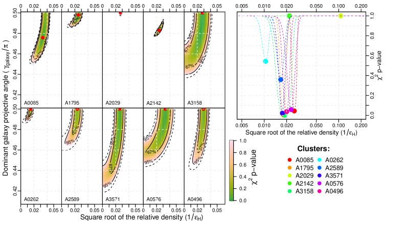
Figure C.2: Observational constraint of the proposed models fitted to RAR of the ten galaxy clusters considered (Li et al., 2023). Left: Best values (red points) and uncertainty area (green shaded regions: 1-$\sigma$ confidence level) of the two parameters ($\varepsilon_{H}$ and $\gamma_{galaxy}$, Table 1) used in fits to individual clusters according to the specific approach (Eq. C15 in C11). Right: Best fits of the single free parameter ($\varepsilon_{H}$) used in the general model (Eq. C16 in C11), defined for $\gamma_{center}=0.48\mathrm{\pi}$. In both cases (1 or 2 free parameters), the projective angle of the neighborhood ($\gamma_{U}$) was fixed to $\gamma_{U}=\mathrm{\pi}/3$. Notice that cluster A2029 did not pass the chi-square test even with the 2-parameter model. However, it passed the test for $\gamma_{U}=0.235\mathrm{\pi}$, corresponding to $\gamma_{U}^{-1}\cos{\gamma_{U}}\approx 1$.

Table 1: Individual fitting of Eq. 4 to each cluster according to the general model (Eq. 5) with one parameter ($\varepsilon_{H}$), and with the specific model for clusters (Eq. 4 with two parameters, $\varepsilon_{H}$ and $\gamma_{galaxy}$). The $p$-values is that of a lower $\chi^{2}$.

Name (data)	General model		Specific model for clusters
	$\varepsilon_{H}$	$\chi^{2}$ $p$-value	$\varepsilon_{H}$	$\gamma_{galaxy}/\mathrm{\pi}$	$\chi^{2}$ $p$-value
A0085 (17)	$40_{-5}^{+6}$	0.04	$31_{-4}^{+5}$	$0.474_{-0.009}^{+0.017}$	$<0.01$
A1795 (4)	$55_{-9}^{+14}$	$<0.01$	$39_{-4}^{+6}$	$0.499_{-0.006}^{+0.001}$	$<0.01$
A2029 (32)	$52_{-20}^{+40}$	$>0.95$	$37_{-10}^{+15}$	$0.500_{-0.002}^{+0}$	$>0.95$
A2142 (31)	$46_{-15}^{+15}$	$>0.95$	$41_{-2}^{+4}$	$0.483_{-0.002}^{+0.003}$	$<0.01$
A3158 (7)	$53_{-17}^{+39}$	$<0.01$	$37_{-8}^{+18}$	$0.491_{-0.030}^{+0.009}$	$<0.01$
A0262 (3)	$96_{-19}^{+32}$	0.54	$67_{-6}^{+10}$	$0.500_{-0.005}^{+0}$	0.57
A2589 (3)	$60_{-14}^{+37}$	0.36	$41_{-4}^{+10}$	$0.500_{-0.013}^{+0}$	0.47
A3571 (3)	$57_{-12}^{+22}$	0.02	$39_{-6}^{+8}$	$0.495_{-0.036}^{+0.005}$	0.14
A0576 (3)	$44_{-11}^{+22}$	0.06	$31_{-6}^{+8}$	$0.493_{-0.023}^{+0.007}$	0.13
A0496 (5)	$50_{-9}^{+16}$	0.04	$33_{-4}^{+6}$	$0.500_{-0.028}^{+0}$	0.14

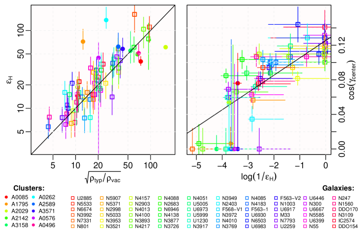
Figure C.3: Model parameters fitted to the 60 high-quality galaxy rotation curves (squares), empirical relationships (black lines), and comparison with the fitting to the RAR data of 10 clusters (circles). Left: Constraint of the 1-parameter HMG model (when $\gamma_{center}=0.48\mathrm{\pi}$ is set, while $\varepsilon_{H}$ is free) for galaxies, which shows an empirical identity between the single parameter $\epsilon_{H}$ and the square root of a relative density $\rho_{typ}/\rho_{vac}$. That is, in units of vacuum density $\rho_{vac}:=3/(8\mathrm{\pi}{G}t^{2})$, an observed density $\rho_{typ}:=\rho(r_{typ})$ is defined at a typical distance of $r_{typ}\sim 50-200\,$kpc, whose fit has been found ($R=0.85$, $p$-value $<0.0001$) as four times the maximum radius ($r_{typ}\approx 4\times r_{max}$) for each galaxy rotation curve, and equal to the minimum radius ($r_{typ}\approx r_{min}$) for the data of each cluster. Right: Constraint on the 2-parameter HMG model for galaxies, which shows a relationship between $\epsilon_{H}$ and $\gamma_{center}$ according to $\cos(\gamma_{center})=\cos(0.460\mathrm{\pi})-0.020\ln(\varepsilon_{H})$ for $1\leq\varepsilon_{H}<400$, with a Pearson coefficient of $R=0.80$ ($p$-value $<0.0001$; black regression line).

References

- Aalbers et al. (2023) Aalbers, J., Akerib, D. S., Akerlof, C. W., et al. 2023, PhRv. Lett., 131, 041002. https://link.aps.org/doi/10.1103/PhysRevLett.131.041002
- Abel et al. (2017) Abel, C., Ayres, N. J., Ban, G., et al. 2017, Physical Review X, 7, 041034
- Ardi & Baumgardt (2020) Ardi, E., & Baumgardt, H. 2020, JPCS, 1503, 012023. https://dx.doi.org/10.1088/1742-6596/1503/1/012023
- Asencio et al. (2022) Asencio, E., Banik, I., Mieske, S., et al. 2022, MNRAS, 515, 2981. https://doi.org/10.1093/mnras/stac1765
- Banik et al. (2023) Banik, I., Pittordis, C., Sutherland, W., et al. 2023, MNRAS, 527, 4573. https://doi.org/10.1093/mnras/stad3393
- Banik & Zhao (2022) Banik, I., & Zhao, H. 2022, Symmetry, 14, doi:10.3390/sym14071331. https://www.mdpi.com/2073-8994/14/7/1331
- Barkana (2018) Barkana, R. 2018, Nature, 555, 71. https://doi.org/10.1038/nature25791
- Batygin et al. (2024) Batygin, K., Morbidelli, A., Brown, M. E., & Nesvorný, D. 2024, ApJ, 966, L8
- Bekenstein (2004) Bekenstein, J. D. 2004, PhRvD, 70, 083509. https://link.aps.org/doi/10.1103/PhysRevD.70.083509
- Blanchet (2007) Blanchet, L. 2007, CQGra, 24, 3529. https://dx.doi.org/10.1088/0264-9381/24/14/001
- Blanchet & Skordis (2024) Blanchet, L., & Skordis, C. 2024, ArXiv e-prints, Arxiv, arXiv:2404.06584
- Brown & Mathur (2023) Brown, K., & Mathur, H. 2023, AJ, 166, 168. https://dx.doi.org/10.3847/1538-3881/acef1e
- Cattaneo et al. (2014) Cattaneo, A., Salucci, P., & Papastergis, E. 2014, ApJ, 783, 66. https://dx.doi.org/10.1088/0004-637X/783/2/66
- Chae (2022) Chae, K.-H. 2022, ApJ, 941, 55. https://dx.doi.org/10.3847/1538-4357/ac93fc
- Chae (2023) —. 2023, ApJ, 952, 128. https://dx.doi.org/10.3847/1538-4357/ace101
- Chae (2024a) —. 2024a, arxiv, doi:10.48550/arXiv.2309.10404. https://doi.org/10.48550/arXiv.2309.10404
- Chae (2024b) —. 2024b, arxiv, doi:10.48550/2402.05720. https://doi.org/10.48550/arXiv.2402.05720
- Chae et al. (2020) Chae, K.-H., Lelli, F., Desmond, H., et al. 2020, ApJ, 904, 51. https://dx.doi.org/10.3847/1538-4357/abbb96
- Ciufolini et al. (2019) Ciufolini, I., Matzner, R., Paolozzi, A., et al. 2019, Scientific Reports, 9, 15881
- Comerón et al. (2023) Comerón, S., Trujillo, I., Cappellari, M., et al. 2023, A&A, 675, A143. https://doi.org/10.1051/0004-6361/202346291
- de Blok et al. (2008) de Blok, W. J. G., Walter, F., Brinks, E., et al. 2008, AJ, 136, 2648. https://dx.doi.org/10.1088/0004-6256/136/6/2648
- De Propris et al. (2020) De Propris, R., West, M. J., Andrade-Santos, F., et al. 2020, MNRAS, 500, 310. https://doi.org/10.1093/mnras/staa3286
- Desmond (2016) Desmond, H. 2016, MNRAS, 464, 4160. https://doi.org/10.1093/mnras/stw2571
- Desmond et al. (2024) Desmond, H., Hees, A., & Famaey, B. 2024, MNRAS, 530, 1781. https://doi.org/10.1093/mnras/stae955
- Di Cintio & Lelli (2015) Di Cintio, A., & Lelli, F. 2015, MNRAS Lett., 456, L127. https://doi.org/10.1093/mnrasl/slv185
- Dittus & Lämmerzahl (2007) Dittus, H., & Lämmerzahl, C. 2007, AdSpR, 39, 244. https://www.sciencedirect.com/science/article/pii/S0273117707001858
- Du et al. (2022) Du, P., Egana-Ugrinovic, D., Essig, R., & Sholapurkar, M. 2022, PhRvX, 12, 011009. https://link.aps.org/doi/10.1103/PhysRevX.12.011009
- Eckert et al. (2022) Eckert, D., Ettori, S., Pointecouteau, E., van der Burg, R. F. J., & Loubser, S. I. 2022, A&A, 662, A123. https://doi.org/10.1051/0004-6361/202142507
- Famaey & McGaugh (2012) Famaey, B., & McGaugh, S. S. 2012, LiRvRe, 15, 10. https://doi.org/10.12942/lrr-2012-10
- Goddy et al. (2023) Goddy, J. S., Stark, D. V., Masters, K. L., et al. 2023, MNRAS, 520, 3895. https://doi.org/10.1093/mnras/stad298
- Harikumar & Biesiada (2022) Harikumar, S., & Biesiada, M. 2022, EuPhJC, 82, 241. https://doi.org/10.1140/epjc/s10052-022-10204-4
- Haslbauer et al. (2020) Haslbauer, M., Banik, I., & Kroupa, P. 2020, MNRAS, 499, 2845. https://doi.org/10.1093/mnras/staa2348
- Hees et al. (2014) Hees, A., Folkner, W. M., Jacobson, R. A., & Park, R. S. 2014, PhRvD, 89, 102002. https://link.aps.org/doi/10.1103/PhysRevD.89.102002
- Hernandez (2023) Hernandez, X. 2023, MNRAS, 525, 1401. https://doi.org/10.1093/mnras/stad2306
- Hernandez et al. (2023) Hernandez, X., Verteletskyi, V., Nasser, L., & Aguayo-Ortiz, A. 2023, MNRAS, 528, 4720. https://doi.org/10.1093/mnras/stad3446
- Hoof et al. (2020) Hoof, S., Geringer-Sameth, A., & Trotta, R. 2020, JCAP, 2020, 012. https://dx.doi.org/10.1088/1475-7516/2020/02/012
- Hu et al. (2024) Hu, X.-S., Zhu, B.-Y., Liu, T.-C., & Liang, Y.-F. 2024, PhRvD, 109, 063036. https://link.aps.org/doi/10.1103/PhysRevD.109.063036
- Katz et al. (2016) Katz, A., Reece, M., & Sajjad, A. 2016, PDU, 12, 24. https://www.sciencedirect.com/science/article/pii/S2212686416000042
- Keenan et al. (2013) Keenan, R. C., Barger, A. J., & Cowie, L. L. 2013, ApJ, 775, 62. https://dx.doi.org/10.1088/0004-637X/775/1/62
- Kroupa (2015) Kroupa, P. 2015, CJP, 93, 169. https://doi.org/10.1139/cjp-2014-0179
- Kroupa et al. (2023) Kroupa, P., Gjergo, E., Asencio, E., et al. 2023, PoS Corfu2022, 436, arXiv:2309.11552. https://doi.org/10.22323/1.436.0231
- Leauthaud et al. (2010) Leauthaud, A., Finoguenov, A., Kneib, J.-P., et al. 2010, ApJ, 709, 97. https://dx.doi.org/10.1088/0004-637X/709/1/97
- Lelli et al. (2016) Lelli, F., McGaugh, S. S., & Schombert, J. M. 2016, ApJ, 152, 157. https://dx.doi.org/10.3847/0004-6256/152/6/157
- Lelli et al. (2019) Lelli, F., McGaugh, S. S., Schombert, J. M., Desmond, H., & Katz, H. 2019, MNRAS, 484, 3267. https://doi.org/10.1093/mnras/stz205
- Lelli et al. (2017) Lelli, F., McGaugh, S. S., Schombert, J. M., & Pawlowski, M. S. 2017, ApJ, 836, 152. https://dx.doi.org/10.3847/1538-4357/836/2/152
- Li et al. (2023) Li, P., Tian, Yong, Júlio, Mariana P., et al. 2023, A&A, 677, A24. https://doi.org/10.1051/0004-6361/202346431
- Liu et al. (2022) Liu, X.-H., Li, Z.-H., Qi, J.-Z., & Zhang, X. 2022, ApJ, 927, 28. https://dx.doi.org/10.3847/1538-4357/ac4c3b
- Mavromatos et al. (2009) Mavromatos, N. E., Sakellariadou, M., & Yusaf, M. F. 2009, PhRvD, 79, 081301. https://link.aps.org/doi/10.1103/PhysRevD.79.081301
- Mazurenko et al. (2023) Mazurenko, S., Banik, I., Kroupa, P., & Haslbauer, M. 2023, MNRAS, 527, 4388. https://doi.org/10.1093/mnras/stad3357
- McGaugh (2004) McGaugh, S. S. 2004, ApJ, 609, 652. https://dx.doi.org/10.1086/421338
- McGaugh et al. (2007) McGaugh, S. S., de Blok, W. J. G., Schombert, J. M., de Naray, R. K., & Kim, J. H. 2007, ApJ, 659, 149. https://dx.doi.org/10.1086/511807
- McGaugh et al. (2016) McGaugh, S. S., Lelli, F., & Schombert, J. M. 2016, PhRvL, 117, 201101. https://link.aps.org/doi/10.1103/PhysRevLett.117.201101
- Merritt (2017) Merritt, D. 2017, Stud. Hist. Philos. Sci. B Stud. Hist. Philos. Modern Phys., 57, 41. https://www.sciencedirect.com/science/article/pii/S1355219816301563
- Migaszewski (2023) Migaszewski, C. 2023, Monthly Notices of the Royal Astronomical Society, 525, 805. https://doi.org/10.1093/mnras/stad2250
- Milgrom (1983) Milgrom, M. 1983, ApJ, 270, 365
- Mitra (2014) Mitra, A. 2014, MNRAS, 442, 382. https://doi.org/10.1093/mnras/stu859
- Moffat & Toth (2009) Moffat, J. W., & Toth, V. T. 2009, MNRAS, 397, 1885. https://doi.org/10.1111/j.1365-2966.2009.14876.x
- Moffat & Toth (2013) —. 2013, Galaxies, 1, 65. https://www.mdpi.com/2075-4434/1/1/65
- Monjo (2017) Monjo, R. 2017, PhRvD, 96, 103505. https://link.aps.org/doi/10.1103/PhysRevD.96.103505
- Monjo (2018) —. 2018, PhRvD, 98, 043508. https://link.aps.org/doi/10.1103/PhysRevD.98.043508
- Monjo (2023) —. 2023, CQGra, 40, 235002. https://iopscience.iop.org/article/10.1088/1361-6382/ad0422
- Monjo (2024a) —. 2024a, ApJ, 965, xx. https://doi.org/xxxx
- Monjo (2024b) —. 2024b, Phd thesis, Complutense University of Madrid, Madrid, Spain, https://10.5281/zenodo.11001487
- Monjo & Campoamor-Stursberg (2020) Monjo, R., & Campoamor-Stursberg, R. 2020, CQGra, 37, 205015. https://dx.doi.org/10.1088/1361-6382/abadaf
- Monjo & Campoamor-Stursberg (2023) —. 2023, CQGra. http://iopscience.iop.org/article/10.1088/1361-6382/aceacc
- Pittordis & Sutherland (2019) Pittordis, C., & Sutherland, W. 2019, MNRAS, 488, 4740. https://doi.org/10.1093/mnras/stz1898
- Pittordis & Sutherland (2023) —. 2023, OJAp, 6, doi:10.21105/astro.2205.02846
- Roshan et al. (2021) Roshan, M., Ghafourian, N., Kashfi, T., et al. 2021, MNRAS, 508, 926. https://doi.org/10.1093/mnras/stab2553
- Seifert (2007) Seifert, M. D. 2007, PhRvD, 76, 064002. https://link.aps.org/doi/10.1103/PhysRevD.76.064002
- Shi et al. (2023) Shi, D., Wang, X., Zheng, X., et al. 2023, arxiv:astro-ph.GA, arXiv.2303.09726, doi:10.48550/arXiv.2303.09726. https://doi.org/10.48550/arXiv.2303.09726
- Skordis & Złośnik (2021) Skordis, C., & Złośnik, T. 2021, Phys. Rev. Lett., 127, 161302. https://link.aps.org/doi/10.1103/PhysRevLett.127.161302
- Stiskalek & Desmond (2023) Stiskalek, R., & Desmond, H. 2023, Monthly Notices of the Royal Astronomical Society, 525, 6130. https://doi.org/10.1093/mnras/stad2675
- Tian et al. (2024) Tian, Y., Ko, C.-M., Li, P., McGaugh, S., & Poblete, S. L. 2024, A&A, 684, A180
- Tian et al. (2020) Tian, Y., Umetsu, K., Ko, C.-M., Donahue, M., & Chiu, I.-N. 2020, ApJ, 896, 70. https://dx.doi.org/10.3847/1538-4357/ab8e3d
- Touboul et al. (2022) Touboul, P., Métris, G., Rodrigues, M., et al. 2022, CQGra, 39, 204009. https://dx.doi.org/10.1088/1361-6382/ac84be
- Trippe (2014) Trippe, S. 2014, Zeitschrift Naturforschung Teil A, 69, 173
- Vokrouhlický et al. (2024) Vokrouhlický, D., Nesvorný, D., & Tremaine, S. 2024, ApJ, in press, arXiv:2403.09555