Distributed Joint User Activity Detection, Channel Estimation, and Data Detection via Expectation Propagation in Cell-Free Massive MIMO

Abstract

We consider the uplink of a grant-free cell-free massive multiple-input multiple-output (GF-CF-MaMIMO) system. We propose an algorithm for distributed joint activity detection, channel estimation, and data detection (JACD) based on expectation propagation (EP) called JACD-EP. We develop the algorithm by factorizing the a posteriori probability (APP) of activities, channels, and transmitted data, then, mapping functions and variables onto a factor graph, and finally, performing a message passing on the resulting factor graph. If users with the same pilot sequence are sufficiently distant from each other, the joint activity detection, channel estimation, and data detection via expectation propagation (JACD-EP) algorithm is able to mitigate the effects of pilot contamination which naturally occurs in grant-free systems due to the large number of potential users and limited signaling resources. Furthermore, it outperforms state-of-the-art algorithms for JACD in grant-free cell-free massive multiple-input multiple-output (GF-CF-MaMIMO) systems.

I Introduction

CF-MaMIMO networks are considered a promising enabler for energy efficient sixth generation (6G) wireless communication systems with ubiquitous coverage and high data rates [1, 2, 3, 4]. Here, a large number of potential user equipments communicate with a central processing unit (CPU) via distributed access points. For sporadic burst traffic as in the Internet-of-Things (IoT), grant-free random access schemes reduce the communication overhead, decoding latency, and enable an efficient resource utilization [5]. In this context, massive multiple-input multiple-output (MaMIMO) are especially well-suited [5] and grant-free cell-free massive multiple-input multiple-output (CF-MaMIMO) (GF-CF-MaMIMO) systems are considered in, e.g., [6, 7]. In GF-CF-MaMIMO, the task of the CPU is to identify the active UEs and estimate their transmitted data. Furthermore, accurate channel estimation is necessary for reliable data detection. However, one major problem in grant-free systems is pilot contamination which naturally occurs due to the large number of UEs and limited signaling resources. Besides, in contrast to centralized MaMIMO, channel hardening and favorable propagation typically do not hold in cell-free systems [8, 9, 10, 11] which further exacerbates the problem of pilot contamination and renders existing pilot decontamination solutions for centralized MaMIMO [12, 13, 14, 15, 16] ineffective. Hence, novel efficient algorithms for JACD are necessary to mitigate pilot contamination in grant-free cell-free systems.

In this work, we propose a novel JACD message-passing algorithm based on EP called JACD-EP. EP is an approximate inference technique which iteratively computes a tractable approximation of a factorized probability distribution by projecting each factor onto an exponential family [17, 18]. The EP algorithm has been already applied, among others, to joint activity detection and channel estimation (JAC) for massive machine-type communications [19] and to joint channel estimation and data detection (JCD) in CF-MaMIMO [20]. For grant-free communication systems, also other approximate inference techniques were considered such as approximate message passing (AMP) which was applied to JAC in [21, 22, 23]. Furthermore, bilinear Gaussian belief propagation (GaBP) was applied in [6] for JACD.

This paper is organized as follows. In Section II, we introduce the GF-CF-MaMIMO system model and formulate the inference problem. In Section III, we present the novel JACD-EP algorithm. Then, the performance of the proposed algorithm is evaluated in Section IV. Finally, some conclusions are drawn.

Notation: Lower case, bold lower case, and bold upper case letters, e.g., $x,\mathbf{x},\mathbf{X}$, represent scalars, vectors and matrices, respectively. $\mathbf{I}_{N}$ is the $N$-dimensional identity matrix. $\mathrm{diag}\!\left\{\cdot\right\}$ is a diagonal matrix with the elements in brackets on the main diagonal. $\delta(\cdot)$ is the Dirac delta function. The indicator function $\mathbbm{1}_{(\cdot)}$ takes value one if the condition in the subscript is satisfied and zero otherwise. $(\cdot)^{T}$ and $(\cdot)^{H}$ denote the transposition and complex conjugate transposition operation, respectively. The trace of a matrix $\mathbf{X}$ is denoted by $\mathrm{tr}\!\left\{\mathbf{X}\right\}$. $|\mathcal{S}|$ stands for the cardinality of the set $\mathcal{S}$. $E\!\left\{\cdot\right\}$ denotes the expectation operator. $\mathcal{CN}\!\left(\mathbf{x}|\boldsymbol{\mu},\mathbf{C}\right)$ represents the circularly-symmetric multivariate complex Gaussian distribution of a complex-valued vector $\mathbf{x}$ with mean $\boldsymbol{\mu}$ and covariance matrix $\mathbf{C}$. $\pi\!\left(x\right)$ denotes the categorical distribution of a discrete random variable $x$. The notation $x\sim p$ indicates that the random variable $x$ follows the distribution $p$. The message sent from the factor node $\Psi_{\alpha}$ to the variable node $\mathbf{x}_{\beta}$ in a factor graph is denoted as $m_{\Psi_{\alpha};\mathbf{x}_{\beta}}$ and consists of parameters of the distribution $p_{\Psi_{\alpha};\mathbf{x}_{\beta}}(\mathbf{x}_{\beta})$ in the exponential family which are denoted with the same subscript of the message, e.g., mean $\boldsymbol{\mu}_{\Psi_{\alpha};\mathbf{x}_{\beta}}$ and covariance matrix $\mathbf{C}_{\Psi_{\alpha};\mathbf{x}_{\beta}}$ for a Gaussian random variable $\mathbf{x}_{\beta}$ with distribution $p_{\Psi_{\alpha};\mathbf{x}_{\beta}}(\mathbf{x}_{\beta})=\mathcal{CN}\!\left(\mathbf{x}|\boldsymbol{\mu}_{\Psi_{\alpha};\mathbf{x}_{\beta}},\mathbf{C}_{\Psi_{\alpha};\mathbf{x}_{\beta}}\right)$ or probability values $\pi_{\Psi_{\alpha};\mathbf{x}_{\beta}}(\mathbf{x}_{\beta})$ for a categorical random variable $\mathbf{x}_{\beta}$ with distribution $p_{\Psi_{\alpha};\mathbf{x}_{\beta}}(\mathbf{x}_{\beta})=\pi_{\Psi_{\alpha};\mathbf{x}_{\beta}}(\mathbf{x}_{\beta})$. The same holds for variable-to-factor messages $m_{\mathbf{x}_{\beta};\Psi_{\alpha}}$.

II System Model

II-A GF-CF-MaMIMO

We consider the uplink of a GF-CF-MaMIMO system with $L$ geographically distributed APs, serving $K$ synchronized single-antenna UEs. Each AP is equipped with $N$ antennas. All APs are connected to a CPU via fronthaul links. Only a fraction of the $K$ UEs are active and transmit data simultaneously. The received signal at the $l^{\text{th}}$ AP at channel use $t$ $\mathbf{y}_{l,t}\in\mathbb{C}^{N\times 1}$ is given by

$$\mathbf{y}_{l,t}=\mathbf{H}_{l}\mathbf{U}\mathbf{x}_{t}+\mathbf{n}_{l,t}=\sum_{k=1}^{K}\mathbf{h}_{l,k}u_{k}x_{kt}+\mathbf{n}_{l,t},$$ (1)

where $\mathbf{H}_{l}=[\mathbf{h}_{l,1}\cdots\mathbf{h}_{l,K}]\!\in\!\mathbb{C}^{N\times K}$ is the channel matrix of AP $l$ and $\mathbf{h}_{l,k}\!\in\!\mathbb{C}^{N\times 1}$ is the channel between AP $l$ and UE $k$; $\mathbf{U}=\mathrm{diag}\!\left\{u_{1},\dots,u_{K}\right\}\in\{0,1\}^{K\times K}$ is the diagonal matrix of user activities whose $k^{\text{th}}$ diagonal element $u_{k}$ is equal to one if UE $k$ is active and zero otherwise; $\mathbf{x}_{t}\in\mathbb{C}^{K\times 1}$ is the transmit vector at channel use $t$ whose $k^{\text{th}}$ entry $x_{kt}$ denotes the transmit symbol of UE $k$ at channel use $t$; and $\mathbf{n}_{l,t}\in\mathbb{C}^{N\times 1}$ is the vector of additive white Gaussian noise (AWGN) at the $l^{\text{th}}$ AP at channel use $t$ with $\mathbf{n}_{l,t}\sim\mathcal{CN}\!\left(\mathbf{n}_{l,t}|\mathbf{0}_{N},\sigma_{n}^{2}\mathbf{I}_{N}\right)$. The channel and the user activity are assumed to be constant during $T$ channel uses which correspond to the channel coherence time. We summarize the receive, transmit, and AWGN vectors over $T$ channel uses in the matrices $\mathbf{Y}_{l}=[\mathbf{y}_{l,1}\cdots\mathbf{y}_{l,T}]\!\in\!\mathbb{C}^{N\times T}$, $\mathbf{X}=[\mathbf{x}_{1}\cdots\mathbf{x}_{T}]\!\in\!\mathbb{C}^{K\times T}$, and $\mathbf{N}_{l}=[\mathbf{n}_{l,1}\cdots\mathbf{n}_{l,T}]\!\in\!\mathbb{C}^{N\times T}$, respectively. The channel between UE $k$ and AP $l$ is assumed to be block Rayleigh fading, i.e., $\mathbf{h}_{l,k}\sim p_{h_{l,k}}(\mathbf{h}_{l,k})=\mathcal{CN}\!\left(\mathbf{h}_{l,k}|\mathbf{0}_{N},\boldsymbol{\Xi}_{l,k}\right)$ where $\boldsymbol{\Xi}_{l,k}\in\mathbb{C}^{N\times N}$ is the spatial correlation matrix and $\xi_{l,k}=\frac{1}{N}\mathrm{tr}\!\left\{\boldsymbol{\Xi}_{l,k}\right\}$ is the large-scale fading coefficient. The activity indicator of user $k$ is drawn from a Bernoulli distribution, $u_{k}\sim p_{u}(u_{k})=(1-\lambda)\mathbbm{1}_{u_{k}=0}+\lambda\mathbbm{1}_{u_{k}=1}$ where $\lambda$ denotes the probability that a user is active. The transmit matrix consists of a pilot matrix $\mathbf{X}^{p}\in\mathbb{C}^{K\times T_{p}}$ with known pilot symbols $x^{p}_{kt}$ and a data matrix $\mathbf{X}^{d}\in\mathcal{X}^{K\times T_{d}}$, i.e., $\mathbf{X}=[\mathbf{X}^{p}\;\mathbf{X}^{d}],$ with $T_{p}+T_{d}=T$ and $\mathcal{X}$ being the transmit symbol constellation of cardinality $M=|\mathcal{X}|$ which does not contain the zero-symbol, i.e., $0\notin\mathcal{X}$. The average symbol transmit power is $\sigma_{x}^{2}=E\!\left\{|x_{kt}|^{2}\right\}$. A similar decomposition holds for the receive matrix, i.e., $\mathbf{Y}_{l}=[\mathbf{Y}^{p}_{l}\;\mathbf{Y}^{d}_{l}]$ with received pilots $\mathbf{Y}^{p}_{l}\in\mathbb{C}^{N\times T_{p}}$ and received data $\mathbf{Y}^{d}_{l}\in\mathbb{C}^{N\times T_{d}}$. Furthermore, the pilot length is much smaller than the number of UEs, $T_{p}\ll K$, since the number of UEs is usually very large and, thus, it is not practical to assign orthogonal pilot sequences to the UEs.

II-B Problem Formulation

The received signals of all APs $l\in\{1,\dots,L\}$ can be summarized in the global equation

$$\mathbf{Y}=\mathbf{H}\mathbf{U}\mathbf{X}+\mathbf{N},$$ (2)

where, for $\mathbf{A}\equiv\{\mathbf{Y},\mathbf{H},\mathbf{N}\}$, $\mathbf{A}=[\mathbf{A}_{1}^{T}\cdots\mathbf{A}_{L}^{T}]^{T}.$ The task of the receiver is to jointly estimate the user activity, channel, and user data matrices $\mathbf{U}$, $\mathbf{H}$, and $\mathbf{X}^{d}$, respectively. The maximum a posteriori (MAP) estimator is given by

$$(\hat{\mathbf{U}},\hat{\mathbf{H}},\hat{\mathbf{X}}^{d})=\mathop{\mathrm{arg\,max}}_{\mathbf{U},\mathbf{H},\mathbf{X}^{d}}\;p_{\text{APP}}(\mathbf{U},\mathbf{H},\mathbf{X}^{d}),$$ (3)

where the APP distribution $p_{\text{APP}}(\mathbf{U},\mathbf{H},\mathbf{X}^{d})$ can be factorized as follows by applying the Bayes theorem,

$$p_{\text{APP}}(\mathbf{U},\mathbf{H},\mathbf{X}^{d}) =p_{U,H,X^{d}|Y,X^{p}}(\mathbf{U},\mathbf{H},\mathbf{X}^{d}|\mathbf{Y},\mathbf{X}^{p})$$

$$\propto p_{Y|U,H,X}(\mathbf{Y}|\mathbf{U},\mathbf{H},\mathbf{X})\cdot p_{U}(\mathbf{U})\cdot p_{H}(\mathbf{H})\cdot p_{X}(\mathbf{X}).$$ (4)

Maximizing (4) with respect to $\mathbf{U}$, $\mathbf{H}$, and $\mathbf{X}^{d}$ is practically not feasible. Hence, in the following section, we propose an inference technique yielding an approximation of $p_{\text{APP}}(\mathbf{U},\mathbf{H},\mathbf{X}^{d})$ for low-complexity JACD.

III JACD-EP Algorithm

In this section we present the proposed JACD-EP algorithm. The algorithm is obtained by introducing a convenient factorization of $p_{\text{APP}}(\mathbf{U},\mathbf{H},\mathbf{X}^{d})$ which induces a factor graph as shown in Section III-A, then selecting parametric representations of distributions from the exponential family to approximate the APP distribution, see Section III-B, and finally, applying EP message-passing rules on a factor graph, e.g., [24, 20], as detailed in Section III-D.

III-A Factor Graph Representation

Similar to [20], to decouple activities, channels, and data of UEs, we introduce the auxiliary variables $\mathbf{g}_{l,k}\coloneq\mathbf{h}_{l,k}u_{k},$ and $\mathbf{z}_{l,kt}\coloneq\mathbf{g}_{l,k}x_{kt}.$ We summarize all auxiliary variables in the matrices $\mathbf{G}$ and $\mathbf{Z}$, respectively. The joint MAP estimator of the user activity, channel, and data as well as the auxiliary variables maximizes the APP distribution given by

$$\begin{split}p_{\text{APP}}(\mathbf{U},\mathbf{H},\mathbf{X}^{d},\mathbf{G},\mathbf{Z})\propto\prod_{l=1}^{L}\prod_{k=1}^{K}\prod_{t=1}^{T}\Big{[}&p(\mathbf{y}_{l,t}|\mathbf{z}_{l,1t},\!...,\mathbf{z}_{l,Kt})\cdot p(\mathbf{z}_{l,kt}|\mathbf{g}_{l,k},x_{kt})\\ &\cdot p(\mathbf{g}_{l,k}|\mathbf{h}_{l,k},u_{k})\cdot\tilde{p}_{u_{k}}(u_{k})\cdot\tilde{p}_{h_{l,k}}(\mathbf{h}_{l,k})\cdot p_{x}(x_{kt})\Big{]},\end{split}$$ (5)

which is factorized by taking into account the independence of channel vectors for different APs and UEs, user activities for different UEs, and data symbols for different UEs and time indices. Furthermore, $\tilde{p}_{u_{k}}(u_{k})$ and $\tilde{p}_{h_{l,k}}(\mathbf{h}_{l,k})$ denote improved prior information of the user activity $u_{k}$ and the channel $\mathbf{h}_{l,k}$, respectively, which can be acquired by a pilot-based initialization algorithm. One possible initialization algorithm is described in Section III-C. We denote the corresponding new prior information for $u_{k}$ and $\mathbf{h}_{l,k}$ by the two probabilities $\tilde{p}_{u_{k}}(0)$ and $\tilde{p}_{u_{k}}(1)$, and the mean vector $\tilde{\boldsymbol{\mu}}_{h_{l,k}}$ and covariance matrix $\tilde{\mathbf{C}}_{h_{l,k}}$, respectively. The probability distributions in (5) are represented by factor nodes (rectangles) in the factor graph illustrated in Fig. 1 and are given by

$$\Psi_{y_{l,t}} \coloneq p(\mathbf{y}_{l,t}|\mathbf{z}_{l,1t},\!...,\mathbf{z}_{l,Kt})=\mathcal{CN}\!\left(\mathbf{y}_{l,t}\Bigg{|}\sum_{k=1}^{K}\mathbf{z}_{l,kt},\sigma_{n}^{2}\mathbf{I}_{N}\right),$$ (6)

$$\Psi_{z_{l,kt}} \coloneq p(\mathbf{z}_{l,kt}|\mathbf{g}_{l,k},x_{kt})=\delta(\mathbf{z}_{l,kt}-\mathbf{g}_{l,k}x_{kt}),$$ (7)

$$\Psi_{g_{l,k}} \coloneq p(\mathbf{g}_{l,k}|\mathbf{h}_{l,k},u_{k})=\delta(\mathbf{g}_{l,k}-\mathbf{h}_{l,k}u_{k}),$$ (8)

$$\Psi_{u_{k}} \coloneq\tilde{p}_{u_{k}}(u_{k})=\tilde{p}_{u_{k}}(0)\mathbbm{1}_{u_{k}=0}+\tilde{p}_{u_{k}}(1)\mathbbm{1}_{u_{k}=1},$$ (9)

$$\Psi_{h_{l,k}} \coloneq\tilde{p}_{h_{l,k}}(\mathbf{h}_{l,k})=\mathcal{CN}\!\left(\mathbf{h}_{l,k}\big{|}\tilde{\boldsymbol{\mu}}_{h_{l,k}},\tilde{\mathbf{C}}_{h_{l,k}}\right),$$ (10)

$$\Psi_{x_{kt}} \coloneq p_{x}(x_{kt})=\begin{cases}{\mathbbm{1}_{x_{kt}=x^{p}_{kt}}}&\text{for }t\leq T_{p},\\ \frac{1}{M}\mathbbm{1}_{x_{kt}\in\mathcal{X}}&\text{for }t>T_{p}.\end{cases}$$ (11)

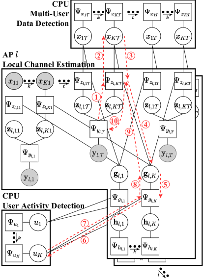
Figure 1: Factor graph for JACD-EP with $\mathcal{T}\coloneq T_{p}+1$. The numbered red dashed arrows show the flow of information according to the scheduling presented in Algorithm 1. Each number corresponds to one message update in Algorithm 1.

The variables in the above equations correspond to variable nodes (circles) in the factor graph. It can be observed that the CPU combines the information from the APs to estimate user activities and data. However, the channels are estimated locally in each AP and there is no need to forward them to the CPU.

III-B EP Approximations and Fronthaul Load

To apply the EP message-passing rules to the factor graph in Fig. 1, we assign a parametric representation of a distribution in the exponential family to each variable node to approximate the corresponding APP distribution. Categorical distributions are chosen for the variables $x_{kt}$ and $u_{k}$ whereas the variables $\mathbf{z}_{l,kt}$, $\mathbf{g}_{l,k}$, and $\mathbf{h}_{l,k}$ are modeled by multivariate complex Gaussian distributions. Thus, messages from and towards $x_{kt}$ for $t>T_{p}$ consist of $M-1$ probabilities while no messages are exchanged for $t\leq T_{p}$ since the pilot symbols are already known. For $u_{k}$, one real value suffices to describe its distribution. Hence, the total fronthaul load per iteration amounts to $2LK(T_{d}(M-1)+1)$ real-valued numbers where the factor two stems from the fact that the messages are sent from the CPU towards the APs and vice versa. Messages involving $\mathbf{z}_{l,kt}$, $\mathbf{g}_{l,k}$, and $\mathbf{h}_{l,k}$ consist of complex-valued vectors and matrices of dimension $N$ and $N\times N$, respectively, which do not contribute to the fronthaul load since they are only processed within an AP.

III-C Initialization, Scheduling, and Estimation

To initialize the JACD-EP algorithm, we apply an algorithm called JAC-EP which is obtained by running the JACD-EP algorithm for the pilot part only, i.e., for $t\leq T_{p}$, with priors $p_{u_{k}}(u_{k})$ and $p_{h_{l,k}}(\mathbf{h}_{l,k})$. This initialization algorithm provides the pilot-based prior information $\tilde{p}_{u_{k}}(u_{k})$ and $\tilde{p}_{h_{l,k}}(\mathbf{h}_{l,k})\equiv(\tilde{\boldsymbol{\mu}}_{h_{l,k}},\tilde{\mathbf{C}}_{h_{l,k}})$ as output. Further details on the joint activity detection and channel estimation via expectation propagation (JAC-EP) algorithm can be found in Appendix A. The soft estimates of the user activities $\tilde{p}_{u_{k}}(u_{k})$ and channels $\tilde{p}_{h_{l,k}}(\mathbf{h}_{l,k})$ are then used as new priors for the JACD-EP algorithm with joint data detection. Furthermore, we need to initialize the messages in JACD-EP. The initial mean vector and covariance matrix of $m_{\Psi_{g_{l,k}};\mathbf{g}_{l,k}}$ and $m_{\mathbf{g}_{l,k};\Psi_{z_{l,kt}}}$ $\forall k,l,t$ are set according to the prior information on $\mathbf{g}_{l,k}$,

$$\boldsymbol{\mu}_{\Psi_{g_{l,k}};\mathbf{g}_{l,k}} =\boldsymbol{\mu}_{\mathbf{g}_{l,k};\Psi_{z_{l,kt}}}=\tilde{p}_{u_{k}}(1)\cdot\tilde{\boldsymbol{\mu}}_{h_{l,k}},$$ (12)

$$\mathbf{C}_{\Psi_{g_{l,k}};\mathbf{g}_{l,k}} =\mathbf{C}_{\mathbf{g}_{l,k};\Psi_{z_{l,kt}}}=\tilde{p}_{u_{k}}(1)\left(\tilde{\mathbf{C}}_{h_{l,k}}+\tilde{\boldsymbol{\mu}}_{h_{l,k}}\tilde{\boldsymbol{\mu}}_{h_{l,k}}^{H}\cdot\tilde{p}_{u_{k}}(0)\right),$$ (13)

and the mean vector and the covariance matrix of $m_{\Psi_{z_{l,kt}};\mathbf{z}_{l,kt}}$ $\forall k,l,t$ according to the prior information on $\mathbf{z}_{l,kt}$,

$$\boldsymbol{\mu}_{\Psi_{z_{l,kt}};\mathbf{z}_{l,kt}} =\mathbf{0},$$ (14)

$$\mathbf{C}_{\Psi_{z_{l,kt}};\mathbf{z}_{l,kt}} =\tilde{p}_{u_{k}}(1)\left(\tilde{\mathbf{C}}_{h_{l,k}}+\tilde{\boldsymbol{\mu}}_{h_{l,k}}\tilde{\boldsymbol{\mu}}_{h_{l,k}}^{H}\right)\sigma_{x}^{2}.$$ (15)

For all other messages, an uninformative initialization is chosen, i.e., a uniform distribution for messages involving categorically distributed variables, and a zero-mean and zero-precision initialization for messages involving Gaussian variables where the precision matrix is the inverse covariance matrix. Then, we update all the messages according to the scheduling given in Algorithm 1 which is illustrated in Fig. 1 as red dashed arrows. Finally, the estimates of the user activities, channels, and data are computed by

$$\hat{u}_{k} =\mathop{\mathrm{arg\,max}}_{u_{k}\in\{0,1\}}\;\hat{p}_{u_{k}}(u_{k}),$$ (16)

$$\hat{\mathbf{h}}_{l,k} =\mathop{\mathrm{arg\,max}}_{\mathbf{h}_{l,k}\in\mathbb{C}^{N}}\;\hat{p}_{\mathbf{h}_{l,k}}(\mathbf{h}_{l,k})=\frac{1}{{Z}_{l,k}}\left(\pi_{u_{k};\Psi_{g_{l,k}}}\!(0)\,\vartheta(0)\,\tilde{\boldsymbol{\mu}}_{h_{l,k}}\!+\pi_{u_{k};\Psi_{g_{l,k}}}\!(1)\,\vartheta(1)\,\check{\boldsymbol{\mu}}_{{l,k};}\right),$$ (17)

$$\hat{x}_{kt} =\mathop{\mathrm{arg\,max}}_{x_{kt}\in\mathcal{X}}\;\hat{p}_{x_{kt}}(x_{kt})\qquad{\text{for }t>T_{p}},$$ (18)

with the approximations of the posterior distributions

$$\hat{p}_{u_{k}}(u_{k}) \propto\tilde{p}_{u_{k}}(u_{k})\cdot\prod_{l=1}^{L}\pi_{\Psi_{g_{l,k}};u_{k}}(u_{k}),$$ (19)

$$\hat{p}_{\mathbf{h}_{l,k}}(\mathbf{h}_{l,k}) \propto\tilde{p}_{h_{l,k}}(\mathbf{h}_{l,k})\cdot\mathcal{CN}\!\left(\mathbf{h}_{l,k}\big{|}\boldsymbol{\mu}_{\Psi_{g_{l,k}};\mathbf{h}_{l,k}},\mathbf{C}_{\Psi_{g_{l,k}};\mathbf{h}_{l,k}}\right),$$ (20)

$$\hat{p}_{x_{kt}}(x_{kt}) \propto\prod_{l=1}^{L}\pi_{\Psi_{z_{l,kt}};x_{kt}}(x_{kt}),$$ (21)

and $\pi_{u_{k};\Psi_{g_{l,k}}}\!(u_{k})$, $\vartheta(u_{k})$, $\check{\boldsymbol{\mu}}_{{l,k};}$, ${Z}_{l,k}$, $\pi_{\Psi_{g_{l,k}};u_{k}}(u_{k})$, $\boldsymbol{\mu}_{\Psi_{g_{l,k}};\mathbf{h}_{l,k}}$, $\mathbf{C}_{\Psi_{g_{l,k}};\mathbf{h}_{l,k}}$, and $\pi_{\Psi_{z_{l,kt}};x_{kt}}(x_{kt})$ defined in Section III-D. The derivation of (17) can be found in (124).

Algorithm 1 JACD-EP Algorithm

0:  Pilot matrix $\mathbf{X}^{p}$, transmit power $\sigma_{x}^{2}$, received signal $\mathbf{Y}$, noise variance $\sigma_{n}^{2}$, prior distributions on user activities $\tilde{p}_{u_{k}}(u_{k})$ and channels $\tilde{p}_{h_{l,k}}(\mathbf{h}_{l,k})$.

0:  Estimated activities $\hat{u}_{k}$, channels $\hat{\mathbf{h}}_{l,k}$, and data $\hat{x}_{kt}$.

1:  $\forall k,l,t$: Initialize $m_{\Psi_{g_{l,k}};\mathbf{g}_{l,k}}$ and $m_{\mathbf{g}_{l,k};\Psi_{z_{l,kt}}}$ via (12), (13), and $m_{\Psi_{z_{l,kt}};\mathbf{z}_{l,kt}}$ via (14), (15).

2:  for $i=1$ to $i_{\text{max}}$ do

3:     $\forall k,l,t$: Update $m_{\Psi_{y_{l,t}};\mathbf{z}_{l,kt}}$ via (22), (23).

4:     $\forall k,l,t\!>\!T_{p}$: Update $m_{\Psi_{z_{l,kt}};x_{kt}}$ via (27).

5:     $\forall k,l,t\!>\!T_{p}$: Update $m_{x_{kt};\Psi_{z_{l,kt}}}$ via (24).

6:     $\forall k,l,t$: Update $m_{\Psi_{z_{l,kt}};\mathbf{g}_{l,k}}$ via (30), (31).

7:     $\forall k,l$: Update $m_{\mathbf{g}_{l,k};\Psi_{g_{l,k}}}$ via (33), (34).

8:     $\forall k,l$: Update $m_{\Psi_{g_{l,k}};u_{k}}$ via (35).

9:     $\forall k,l$: Update $m_{u_{k};\Psi_{g_{l,k}}}$ via (32).

10:     $\forall k,l$: Update $m_{\Psi_{g_{l,k}};\mathbf{g}_{l,k}}$ via (36), (37).

11:     $\forall k,l,t$: Update $m_{\mathbf{g}_{l,k};\Psi_{z_{l,kt}}}$ via (25), (26).

12:     $\forall k,l,t$: Update $m_{\Psi_{z_{l,kt}};\mathbf{z}_{l,kt}}$ via (28), (29).

13:  return  $\hat{u}_{k}$ calculated via (16) $\forall k$.

14:  return  $\hat{\mathbf{h}}_{l,k}$ calculated via (17) $\forall k,l$.

15:  return  $\hat{x}_{kt}$ calculated via (18) $\forall k,{t>T_{p}}$.

As in [20, 24], we apply damping to the factor-to-variable messages with damping parameter $\eta\in[0,1]$, i.e., the updated parameter of a factor-to-variable message is a convex combination of the old parameter and the new parameter. For example, the updated message $\pi_{\Psi_{g_{l,k}};u_{k}}(u_{k})$ in line 8 of Algorithm 1 is given by $\pi_{\Psi_{g_{l,k}};u_{k}}(u_{k})=\eta\cdot\pi_{\text{new}}+(1-\eta)\cdot\pi_{\text{old}}$, where $\pi_{\text{new}}$ is computed according to (35) and $\pi_{\text{old}}$ is the message $\pi_{\Psi_{g_{l,k}};u_{k}}(u_{k})$ from the previous iteration. For the Gaussian factor-to-variable messages, we apply damping to the natural parameters of the Gaussian distribution $\mathcal{CN}\!\left(\mathbf{x}|\boldsymbol{\mu},\mathbf{C}\right)$, i.e., the precision matrix $\boldsymbol{\Lambda}=\mathbf{C}^{-1}$ and the transformed mean vector $\boldsymbol{\gamma}=\mathbf{C}^{-1}\boldsymbol{\mu}$. Furthermore, we update the parameters of $m_{\Psi_{z_{l,kt}};\mathbf{g}_{l,k}}$, $m_{\Psi_{g_{l,k}};\mathbf{g}_{l,k}}$, and $m_{\Psi_{z_{l,kt}};\mathbf{z}_{l,kt}}$ in line 6, 10, and 12 of Algorithm 1 only if the new covariance matrix obtained by (30), (36), and (28), respectively, is symmetric positive definite. Otherwise, we keep the parameters from the previous iteration.

III-D Message-Passing Update Rules

In this section, we present the EP message-passing update rules for the factor graph in Fig. 1. Detailed derivations can be found in Appendix D. The mean vector $\boldsymbol{\mu}$ and the covariance matrix $\mathbf{C}$ of a Gaussian random variable can be readily expressed by the natural parameters $\boldsymbol{\gamma}\!=\!\mathbf{C}^{-1}\boldsymbol{\mu}$ and $\boldsymbol{\Lambda}\!=\!\mathbf{C}^{-1}$. In the following, we will switch between these two representations without explicitly mentioning the transformation, e.g., if $\boldsymbol{\mu}_{\Psi_{\alpha};\mathbf{x}_{\beta}}$ and $\mathbf{C}_{\Psi_{\alpha};\mathbf{x}_{\beta}}$ are computed, then $\boldsymbol{\gamma}_{\Psi_{\alpha};\mathbf{x}_{\beta}}$ and $\boldsymbol{\Lambda}_{\Psi_{\alpha};\mathbf{x}_{\beta}}$ are automatically given and vice versa.

Update of $m_{\Psi_{y_{l,t}};\mathbf{z}_{l,kt}}$ (cf. (80), (81)):

$$\boldsymbol{\mu}_{\Psi_{y_{l,t}};\mathbf{z}_{l,kt}} =\mathbf{y}_{l,t}-\sum_{k^{\prime}\neq k}\boldsymbol{\mu}_{\Psi_{z_{l,k^{\prime}t}};\mathbf{z}_{l,k^{\prime}t}},$$ (22)

$$\mathbf{C}_{\Psi_{y_{l,t}};\mathbf{z}_{l,kt}} =\sigma_{n}^{2}\mathbf{I}_{N}+\sum_{k^{\prime}\neq k}\mathbf{C}_{\Psi_{z_{l,k^{\prime}t}};\mathbf{z}_{l,k^{\prime}t}}.$$ (23)

Update of $m_{x_{kt};\Psi_{z_{l,kt}}}$ (cf. (82)):

$$\pi_{x_{kt};\Psi_{z_{l,kt}}}(x_{kt})\propto\prod_{l^{\prime}\neq l}\pi_{\Psi_{z_{l^{\prime},kt}};x_{kt}}(x_{kt}).$$ (24)

Update of $m_{\mathbf{g}_{l,k};\Psi_{z_{l,kt}}}$ (cf. (85), (86)):

$$\boldsymbol{\Lambda}_{\mathbf{g}_{l,k};\Psi_{z_{l,kt}}} =\boldsymbol{\Lambda}_{\Psi_{g_{l,k}};\mathbf{g}_{l,k}}+\sum_{t^{\prime}\neq t}\boldsymbol{\Lambda}_{\Psi_{z_{l,kt^{\prime}}};\mathbf{g}_{l,k}},$$ (25)

$$\boldsymbol{\gamma}_{\mathbf{g}_{l,k};\Psi_{z_{l,kt}}} =\boldsymbol{\gamma}_{\Psi_{g_{l,k}};\mathbf{g}_{l,k}}+\sum_{t^{\prime}\neq t}\boldsymbol{\gamma}_{\Psi_{z_{l,kt^{\prime}}};\mathbf{g}_{l,k}}.$$ (26)

Update of $m_{\Psi_{z_{l,kt}};x_{kt}}$ (cf. (90)):

$$\pi_{\Psi_{z_{l,kt}};x_{kt}}(x_{kt})\propto\theta(x_{kt}),$$ (27)

with

$$\theta(x_{kt})=\mathcal{CN}(\mathbf{0}|\boldsymbol{\mu}_{\Psi_{y_{l,t}};\mathbf{z}_{l,kt}}-\boldsymbol{\mu}_{\mathbf{g}_{l,k};\Psi_{z_{l,kt}}}x_{kt}\mathbf{C}_{\Psi_{y_{l,t}};\mathbf{z}_{l,kt}}+\mathbf{C}_{\mathbf{g}_{l,k};\Psi_{z_{l,kt}}}|x_{kt}|^{2}).$$

Update of $m_{\Psi_{z_{l,kt}};\mathbf{z}_{l,kt}}$ (cf. (99), (100)):

$$\boldsymbol{\Lambda}_{\Psi_{z_{l,kt}};\mathbf{z}_{l,kt}} =\hat{\boldsymbol{\Lambda}}_{1_{l,kt};}-\boldsymbol{\Lambda}_{\Psi_{y_{l,t}};\mathbf{z}_{l,kt}},$$ (28)

$$\boldsymbol{\gamma}_{\Psi_{z_{l,kt}};\mathbf{z}_{l,kt}} =\hat{\boldsymbol{\gamma}}_{1_{l,kt};}-\boldsymbol{\gamma}_{\Psi_{y_{l,t}};\mathbf{z}_{l,kt}},$$ (29)

with $\hat{\boldsymbol{\mu}}_{1_{l,kt};}\!\!=\!\check{\boldsymbol{\mu}}_{{l,kt};}(x_{kt})$, $\hat{\mathbf{C}}_{1_{l,kt};}\!\!=\!\check{\mathbf{C}}_{{l,kt};}(x_{kt})$ for $t\leq T_{p}$ and

$$\hat{\boldsymbol{\mu}}_{1_{l,kt};} =\frac{1}{{Z}_{{l,kt}}}\sum_{x_{kt}\in\mathcal{X}}\pi_{x_{kt};\Psi_{z_{l,kt}}}(x_{kt})\cdot\theta(x_{kt})\cdot\check{\boldsymbol{\mu}}_{{l,kt};}(x_{kt}),$$

$$\hat{\mathbf{C}}_{1_{l,kt};} =\frac{1}{{Z}_{{l,kt}}}\sum_{x_{kt}\in\mathcal{X}}\pi_{x_{kt};\Psi_{z_{l,kt}}}(x_{kt})\cdot\theta(x_{kt})\cdot\big{(}\check{\mathbf{C}}_{{l,kt};}(x_{kt})+\check{\boldsymbol{\mu}}_{{l,kt};}(x_{kt})\cdot\check{\boldsymbol{\mu}}_{{l,kt};}^{H}(x_{kt})\big{)}-\hat{\boldsymbol{\mu}}_{1_{l,kt};}\hat{\boldsymbol{\mu}}_{1_{l,kt};}^{H},$$

for $t>T_{p}$ with

$${Z}_{{l,kt}} =\sum_{x_{kt}\in\mathcal{X}}\pi_{x_{kt};\Psi_{z_{l,kt}}}(x_{kt})\cdot\theta(x_{kt}),$$

$$\check{\boldsymbol{\Lambda}}_{{l,kt};}(x_{kt}) =\boldsymbol{\Lambda}_{\Psi_{y_{l,t}};\mathbf{z}_{l,kt}}+\boldsymbol{\Lambda}_{\mathbf{g}_{l,k};\Psi_{z_{l,kt}}}|x_{kt}|^{-2},$$

$$\check{\boldsymbol{\gamma}}_{{l,kt};}(x_{kt}) =\boldsymbol{\gamma}_{\Psi_{y_{l,t}};\mathbf{z}_{l,kt}}+\boldsymbol{\gamma}_{\mathbf{g}_{l,k};\Psi_{z_{l,kt}}}\frac{x_{kt}}{|x_{kt}|^{2}}.$$

Update of $m_{\Psi_{z_{l,kt}};\mathbf{g}_{l,k}}$ (cf. (108), (109)):

$$\boldsymbol{\Lambda}_{\Psi_{z_{l,kt}};\mathbf{g}_{l,k}} =\hat{\boldsymbol{\Lambda}}_{2_{l,kt};}-\boldsymbol{\Lambda}_{\mathbf{g}_{l,k};\Psi_{z_{l,kt}}},$$ (30)

$$\boldsymbol{\gamma}_{\Psi_{z_{l,kt}};\mathbf{g}_{l,k}} =\hat{\boldsymbol{\gamma}}_{2_{l,kt};}-\boldsymbol{\gamma}_{\mathbf{g}_{l,k};\Psi_{z_{l,kt}}},$$ (31)

with $\hat{\boldsymbol{\mu}}_{2_{l,kt};}=\frac{\check{\boldsymbol{\mu}}_{{l,kt};}(x_{kt})}{x_{kt}}$, $\hat{\mathbf{C}}_{2_{l,kt};}=\frac{\check{\mathbf{C}}_{{l,kt};}(x_{kt})}{|x_{kt}^{2}|}$ for $t\leq T_{p}$ and

$$\hat{\boldsymbol{\mu}}_{2_{l,kt};} =\frac{1}{{Z}_{l,kt}}\sum_{x_{kt}\in\mathcal{X}}\pi_{x_{kt};\Psi_{z_{l,kt}}}(x_{kt})\cdot\frac{\theta(x_{kt})}{x_{kt}}\cdot\check{\boldsymbol{\mu}}_{{l,kt};}(x_{kt}),$$

$$\hat{\mathbf{C}}_{2_{l,kt};} =\frac{1}{{Z}_{{l,kt}}}\sum_{x_{kt}\in\mathcal{X}}\pi_{x_{kt};\Psi_{z_{l,kt}}}(x_{kt})\cdot\frac{\theta(x_{kt})}{|x_{kt}^{2}|}\cdot\big{(}\check{\mathbf{C}}_{{l,kt};}(x_{kt})+\check{\boldsymbol{\mu}}_{{l,kt};}(x_{kt})\cdot\check{\boldsymbol{\mu}}_{{l,kt};}^{H}(x_{kt})\big{)}-\hat{\boldsymbol{\mu}}_{{l,kt};}\hat{\boldsymbol{\mu}}_{{l,kt};}^{H},$$

for $t>T_{p}$ with ${Z}_{{l,kt}},\check{\boldsymbol{\Lambda}}_{{l,kt};}(x_{kt}),\check{\boldsymbol{\gamma}}_{{l,kt};}(x_{kt})$ given before.

Update of $m_{u_{k};\Psi_{g_{l,k}}}$ (cf. (110)):

$$\pi_{u_{k};\Psi_{g_{l,k}}}(u_{k})\propto\tilde{p}_{u_{k}}(u_{k})\cdot\prod_{l^{\prime}\neq l}\pi_{\Psi_{g_{l^{\prime},k}};u_{k}}(u_{k}),$$ (32)

Update of $m_{\mathbf{g}_{l,k};\Psi_{g_{l,k}}}$ (cf. (113), (114)):

$$\boldsymbol{\Lambda}_{\mathbf{g}_{l,k};\Psi_{g_{l,k}}} =\sum_{t=1}^{T}\boldsymbol{\Lambda}_{\Psi_{z_{l,kt}};\mathbf{g}_{l,k}},$$ (33)

$$\boldsymbol{\gamma}_{\mathbf{g}_{l,k};\Psi_{g_{l,k}}} =\sum_{t=1}^{T}\boldsymbol{\gamma}_{\Psi_{z_{l,kt}};\mathbf{g}_{l,k}}.$$ (34)

Update of $m_{\Psi_{g_{l,k}};u_{k}}$ (cf. (118)):

$$\pi_{\Psi_{g_{l,k}};u_{k}}(u_{k})\propto\vartheta(u_{k}),$$ (35)

with

$$\vartheta(u_{k})=\mathcal{CN}(\mathbf{0}|\boldsymbol{\mu}_{\mathbf{g}_{l,k};\Psi_{g_{l,k}}}\!\!\!-\tilde{\boldsymbol{\mu}}_{h_{l,k}}u_{k},\mathbf{C}_{\mathbf{g}_{l,k};\Psi_{g_{l,k}}}\!\!\!+\tilde{\mathbf{C}}_{h_{l,k}}u_{k}).$$

Update of $m_{\Psi_{g_{l,k}};\mathbf{g}_{l,k}}$ (cf. (136), (137)):

$$\boldsymbol{\Lambda}_{\Psi_{g_{l,k}};\mathbf{g}_{l,k}} =\hat{\boldsymbol{\Lambda}}_{{l,k};}-\boldsymbol{\Lambda}_{\mathbf{g}_{l,k};\Psi_{g_{l,k}}},$$ (36)

$$\boldsymbol{\gamma}_{\Psi_{g_{l,k}};\mathbf{g}_{l,k}} =\hat{\boldsymbol{\gamma}}_{{l,k};}-\boldsymbol{\gamma}_{\mathbf{g}_{l,k};\Psi_{g_{l,k}}},$$ (37)

with

$$\hat{\boldsymbol{\mu}}_{{l,k};} =\frac{1}{{Z}_{{l,k}}}\!\cdot\!\pi_{u_{k};\Psi_{g_{l,k}}}\!(1)\cdot\vartheta(1)\cdot\check{\boldsymbol{\mu}}_{{l,k};},$$

$$\hat{\mathbf{C}}_{{l,k};} =\frac{1}{{Z}_{{l,k}}}\!\cdot\!\pi_{u_{k};\Psi_{g_{l,k}}}\!(1)\cdot\vartheta(1)\cdot(\check{\mathbf{C}}_{{l,k};}\!+\!\check{\boldsymbol{\mu}}_{{l,k};}\check{\boldsymbol{\mu}}_{{l,k};}^{H})\!-\!\hat{\boldsymbol{\mu}}_{{l,k};}\hat{\boldsymbol{\mu}}_{{l,k};}^{H}.$$

$${Z}_{{l,k}} =\pi_{u_{k};\Psi_{g_{l,k}}}(0)\cdot\vartheta(0)+\pi_{u_{k};\Psi_{g_{l,k}}}(1)\cdot\vartheta(1)$$

$$\check{\boldsymbol{\Lambda}}_{{l,k};} =\boldsymbol{\Lambda}_{\mathbf{g}_{l,k};\Psi_{g_{l,k}}}+\tilde{\boldsymbol{\Lambda}}_{h_{l,k}},$$

$$\check{\boldsymbol{\gamma}}_{{l,k};} =\boldsymbol{\gamma}_{\mathbf{g}_{l,k};\Psi_{g_{l,k}}}+\tilde{\boldsymbol{\gamma}}_{h_{l,k}}.$$

III-E Modification for Pilot Contamination

Since the number of UEs is larger than the pilot sequence length, pilot contamination will naturally occur and degrade the performance. In the following, we propose a simple heuristic approach to account for pilot contamination. The efficacy of the proposed approach was verified via simulations.

The adverse effect of pilot contamination is particularly pronounced for UEs that share the same pilot sequence and are close to each other. For these cases, we propose to add a correction term to the covariance matrix in (23) for $t\leq T_{p}$ when generating the prior information via the pilot-based JAC-EP initialization algorithm. We denote the set of UEs which use the same pilot sequence as UE $k$ by $\mathcal{P}_{k}.$ Then, the covariance matrix with the correction term is given by

$$\mathbf{C}_{\Psi_{y_{l,t}};\mathbf{z}_{l,kt}}=\sigma_{n}^{2}\mathbf{I}_{N}+\sum_{k^{\prime}\in\mathcal{P}_{k}}\boldsymbol{\Xi}_{l,k}|x^{p}_{k^{\prime}t}|^{2}+\sum_{k^{\prime}\neq k}\mathbf{C}_{\Psi_{z_{l,k^{\prime}t}};\mathbf{z}_{l,k^{\prime}t}}.$$ (38)

IV Numerical Results

In this section, we analyze the performance of the JACD-EP algorithm via Monte Carlo simulations.

IV-A Simulation Setup

We consider a network of size $400\times 400\,$m with $L=16$ APs placed on a regular grid at the following positions $\{(50+i\!\cdot\!100,50+j\!\cdot\!100)\,\text{m}\,|\,i,j\in\{0,1,2,3\}\}$ and a height of 10 m. On the ground, $K=16$ UEs are deployed according to a uniform point process (UPP). We consider 100 different outcomes of the UPP. For each UPP outcome, the large-scale fading coefficients are deterministic and computed according to the 3GPP urban microcell model [25] whereas for the random variables, i.e., small-scale fading coefficients, activities, and pilot sequences, we generate $10^{3}$ realizations. This allows us to analyze the quality of service (QoS) distribution in the network. The activity probability of all users is set to $\lambda=0.5$, and the transmit power is $\sigma_{x}^{2}=16\,$dBm. Furthermore, random binary phase-shift-keying (BPSK) pilot sequences of length $T_{p}=8$ are utilized and $T_{d}=\{10,30\}$ 4- quadrature amplitude modulation (QAM) symbols are transmitted during the data transmission phase. The noise power at each AP is set to $\sigma_{n}^{2}=-96\,$dBm. As benchmark schemes, we consider the centralized linear minimum mean squared error (MMSE) data detector and the GaBP algorithm in [6]. Both of these schemes are initialized by the multiple measurement vector AMP (MMV-AMP) algorithm in [22]. Besides, we consider the genie-aided centralized linear MMSE detector with perfect UE activity and channel knowledge. For all iterative algorithms, the damping parameter is $\eta=0.5$. Furthermore, the maximum number of iterations for the multiple measurement vector approximate message passing (MMV-AMP) algorithm is set to 200, whereas the GaBP- and EP-based algorithms perform 20 iterations.

IV-B Performance Metrics and Results

For assessing the user activity detection, channel estimation, and data detection performance, we consider the empirical cumulative distribution functions of the detection error rate (DER), the normalized mean squared error (NMSE), and the symbol error rate (SER), respectively. The empirical CDFs are obtained considering all UEs in each UPP outcome whereas DER, NMSE, and SER are computed by averaging over the $10^{3}$ small-scale fading and UE activity realizations generated for each UPP outcome. The DER is defined as the ratio of the number of erroneously classified UE activities and the total number of UE activity realizations, i.e., $\text{DER}\coloneq E\!\left\{\mathbbm{1}_{\hat{u}_{k}\neq u_{k}}\right\}$, and includes both miss detections and false alarms. The corresponding simulation results are illustrated in Fig. 2a. The NMSE and SER are considered naturally for active users only, i.e., $\text{NMSE}\coloneq E\!\left\{\frac{||\hat{\mathbf{h}}_{k}-\mathbf{h}_{k}||}{||\mathbf{h}_{k}||}\;\big{|}\;u_{k}=1\right\}$, $\text{SER}\coloneq E\!\left\{\mathbbm{1}_{\hat{x}_{kt}\neq x_{kt}}\;|\;u_{k}=1,t>T_{p}\right\}$. Furthermore, in the computation of the NMSE, we neglect weak channels, i.e., channels whose large-scale fading coefficient multiplied by the transmit power is smaller than the noise power at the APs, to avoid taking into account errors on weak and insignificant channels. The channel estimation and data detection performance is depicted in Figs. 2b and 2c, respectively.

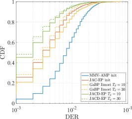
(a) CDF of DER.

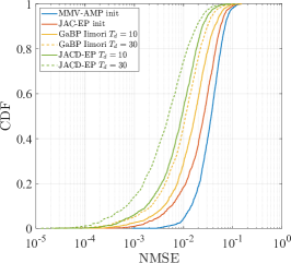
(b) CDF of NMSE.

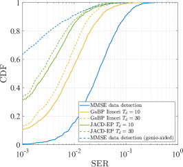
(c) CDF of SER.

Figure 2: Numerical results for $L=16$, $N=1$, $K=16$, $\lambda=0.5$, $T_{p}=8$, $T_{d}=\{10,30\}$, and random BPSK pilots.

The results illustrate the advantages of using jointly pilot and data sequences for both data and activity detection and the superior performance of the JACD-EP algorithm compared to state-of-the-art benchmark schemes. Furthermore, it can be observed that an increase of the data length improves the performance with respect to all considered metrics.

V Conclusion

In this paper, we considered the uplink of a GF-CF-MaMIMO system and tackled the problem of JACD. We developed the JACD-EP algorithm by applying EP message passing on a factor graph where we considered accurate categorical probability distributions for user activity and data, and Gaussian probability distributions for the channels. The proposed algorithm is robust against pilot contamination and outperforms state-of-the-art algorithms in terms of DER, NMSE, and SER.

Appendix A JAC-EP Initialization Algorithm

The JAC-EP algorithm can be obtained by running the JACD-EP algorithm for the pilot part only, i.e., for $t\leq T_{p}$, with priors $p_{u_{k}}(u_{k})$ and $p_{h_{l,k}}(\mathbf{h}_{l,k})$. However, since we do not have to estimate the symbols $x_{kt}$ during initialization, the factorization of the APP and the corresponding factor graph and algorithm simplify. In the following, we describe the simplified JAC-EP algorithm in more detail. We use the same system model and notation as in the main body of this document except that we only consider signals in the pilot phase, i.e., $1\leq t\leq T_{p}$.

A-A Factor Graph Representation

The task of the JAC-EP algorithm is to find initial estimates on the user activities and channels. Hence, the factorized APP distribution with auxiliary variables $\mathbf{g}_{l,k}\coloneq\mathbf{h}_{l,k}u_{k}$ is given by

$$\begin{split}p_{\text{APP}}(\mathbf{U},\mathbf{H},\mathbf{G})\propto\prod_{l=1}^{L}\prod_{k=1}^{K}\prod_{t=1}^{T_{p}}\Big{[}&p(\mathbf{y}_{l,t}|\mathbf{g}_{l,1},\!...,\mathbf{g}_{l,K})\cdot p(\mathbf{g}_{l,k}|\mathbf{h}_{l,k},u_{k})\cdot p_{u_{k}}(u_{k})\cdot p_{h_{l,k}}(\mathbf{h}_{l,k})\Big{]}.\end{split}$$ (39)

In contrast to (5), the auxiliary variables $\mathbf{z}_{l,kt}$ are irrelevant since the pilot symbols $x_{kt}$ are assumed to be known. The probability distributions in (39) are given by

$$\Psi_{y_{l,t}} \coloneq p(\mathbf{y}_{l,t}|\mathbf{g}_{l,1},\!...,\mathbf{g}_{l,K})=\mathcal{CN}\!\left(\mathbf{y}_{l,t}\Bigg{|}\sum_{k=1}^{K}\mathbf{g}_{l,k}x_{kt},\sigma_{n}^{2}\mathbf{I}_{N}\right),$$ (40)

$$\Psi_{g_{l,k}} \coloneq p(\mathbf{g}_{l,k}|\mathbf{h}_{l,k},u_{k})=\delta(\mathbf{g}_{l,k}-\mathbf{h}_{l,k}u_{k}),$$ (41)

$$\Psi_{u_{k}} \coloneq p_{u_{k}}(u_{k})=(1-\lambda)\mathbbm{1}_{u_{k}=0}+\lambda\mathbbm{1}_{u_{k}=1},$$ (42)

$$\Psi_{h_{l,k}} \coloneq p_{h_{l,k}}(\mathbf{h}_{l,k})=\mathcal{CN}\!\left(\mathbf{h}_{l,k}\big{|}\mathbf{0},\boldsymbol{\Xi}_{l,k}\right).$$ (43)

The corresponding factor graph is illustrated in Fig. 3.

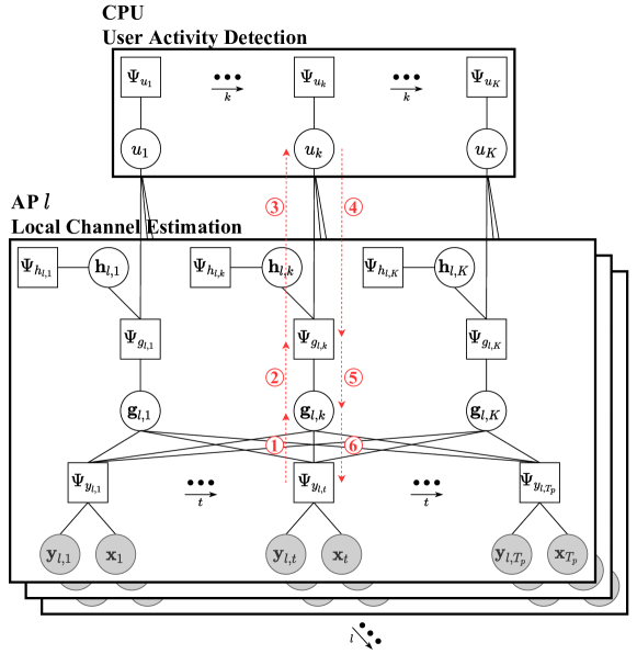
Figure 3: Factor graph for JAC-EP. The numbered red dashed arrows show the flow of information according to the scheduling presented in Algorithm 2. Each number corresponds to one message update in Algorithm 2.

A-B EP Approximations and Fronthaul Load

We choose the same approximate exponential family distributions for the variable nodes as in the JACD-EP algorithm, i.e., activities $u_{k}$ are modeled by categorical distributions whereas auxiliary variables $\mathbf{g}_{l,k}$ and channels $\mathbf{h}_{l,k}$ are modeled by multivariate complex Gaussian distributions. Therefore, messages from and towards $u_{k}$ consist of one probability value which yields a fronthaul load of $2LK$ real-valued numbers. Messages involving $\mathbf{g}_{l,k}$ and $\mathbf{h}_{l,k}$ consist of complex-valued vectors and matrices of dimension $N$ and $N\times N$, respectively, which do not contribute to the fronthaul load since they are only processed within an AP.

A-C Initialization, Scheduling, and Estimation

As indicated in Appendix A-A, the prior distributions $p_{u_{k}}(u_{k})$ and $p_{h_{l,k}}(\mathbf{h}_{l,k})$ are used for initializing the JAC-EP algorithm. The initial mean vector and covariance matrix of $m_{\Psi_{g_{l,k}};\mathbf{g}_{l,k}}$ and $m_{\mathbf{g}_{l,k};\Psi_{y_{l,t}}}$ $\forall k,l,t\leq T_{p}$ are set according to the prior information on $\mathbf{g}_{l,k}$,

$$\boldsymbol{\mu}_{\Psi_{g_{l,k}};\mathbf{g}_{l,k}} =\boldsymbol{\mu}_{\mathbf{g}_{l,k};\Psi_{y_{l,t}}}=\mathbf{0},$$ (44)

$$\mathbf{C}_{\Psi_{g_{l,k}};\mathbf{g}_{l,k}} =\mathbf{C}_{\mathbf{g}_{l,k};\Psi_{y_{l,t}}}=\lambda\cdot\boldsymbol{\Xi}_{l,k}.$$ (45)

For all other messages, an uninformative initialization is chosen. Then, we update all the messages according to the scheduling given in Algorithm 2 which is illustrated in Fig. 3 as red dashed arrows. Finally, the estimates of the user activities and channels are computed by

$$\hat{u}_{k} =\mathop{\mathrm{arg\,max}}_{u_{k}\in\{0,1\}}\;\hat{p}_{u_{k}}(u_{k}),$$ (46)

$$\hat{\mathbf{h}}_{l,k} =\mathop{\mathrm{arg\,max}}_{\mathbf{h}_{l,k}\in\mathbb{C}^{N}}\;\hat{p}_{\mathbf{h}_{l,k}}(\mathbf{h}_{l,k})=\frac{1}{{Z}_{l,k}}\pi_{u_{k};\Psi_{g_{l,k}}}\!(1)\,\vartheta(1)\,\check{\boldsymbol{\mu}}_{{l,k};},$$ (47)

with the approximations of the posterior distributions

$$\hat{p}_{u_{k}}(u_{k}) \propto p_{u_{k}}(u_{k})\cdot\prod_{l=1}^{L}\pi_{\Psi_{g_{l,k}};u_{k}}(u_{k}),$$ (48)

$$\hat{p}_{\mathbf{h}_{l,k}}(\mathbf{h}_{l,k}) \propto p_{h_{l,k}}(\mathbf{h}_{l,k})\cdot\mathcal{CN}\!\left(\mathbf{h}_{l,k}\big{|}\boldsymbol{\mu}_{\Psi_{g_{l,k}};\mathbf{h}_{l,k}},\mathbf{C}_{\Psi_{g_{l,k}};\mathbf{h}_{l,k}}\right).$$ (49)

and $\pi_{u_{k};\Psi_{g_{l,k}}}\!(u_{k})$, $\vartheta(u_{k})$, $\check{\boldsymbol{\mu}}_{{l,k};}$, ${Z}_{l,k}$, $\pi_{\Psi_{g_{l,k}};u_{k}}(u_{k})$, $\boldsymbol{\mu}_{\Psi_{g_{l,k}};\mathbf{h}_{l,k}}$, and $\mathbf{C}_{\Psi_{g_{l,k}};\mathbf{h}_{l,k}}$ defined in Appendix A-D. The derivation of (47) can be found in (162).

Algorithm 2 JAC-EP Algorithm

0:  Pilot matrix $\mathbf{X}^{p}$, received pilot signal $\mathbf{Y}^{p}$, noise variance $\sigma_{n}^{2}$, user activity probability $\lambda$, channel correlation matrices $\boldsymbol{\Xi}_{l,k}$.

0:  Estimated activities $\hat{u}_{k}$ and channels $\hat{\mathbf{h}}_{l,k}$.

1:  $\forall k,l,t\leq T_{p}$: Initialize $m_{\Psi_{g_{l,k}};\mathbf{g}_{l,k}}$ and $m_{\mathbf{g}_{l,k};\Psi_{y_{l,t}}}$ via (44), (45).

2:  for $i=1$ to $i_{\text{max}}$ do

3:     $\forall k,l,t\leq T_{p}$: Update $m_{\Psi_{y_{l,t}};\mathbf{g}_{l,k}}$ via (52), (53)$/$(54).

4:     $\forall k,l$: Update $m_{\mathbf{g}_{l,k};\Psi_{g_{l,k}}}$ via (56), (57).

5:     $\forall k,l$: Update $m_{\Psi_{g_{l,k}};u_{k}}$ via (58).

6:     $\forall k,l$: Update $m_{u_{k};\Psi_{g_{l,k}}}$ via (55).

7:     $\forall k,l$: Update $m_{\Psi_{g_{l,k}};\mathbf{g}_{l,k}}$ via (59), (60).

8:     $\forall k,l,t\leq T_{p}$: Update $m_{\mathbf{g}_{l,k};\Psi_{y_{l,t}}}$ via (50), (51).

9:  return  $\hat{u}_{k}$ calculated via (46) $\forall k$.

10:  return  $\hat{\mathbf{h}}_{l,k}$ calculated via (47) $\forall k,l$.

As in the JACD-EP algorithm, we apply damping to the factor-to-variable messages with damping parameter $\eta\in[0,1]$ Furthermore, we update the parameters of $m_{\Psi_{g_{l,k}};\mathbf{g}_{l,k}}$ in line 7 of Algorithm 2 only if the new covariance matrix obtained by (59) is symmetric positive definite. Otherwise, we keep the parameters from the previous iteration.

A-D Message-Passing Update Rules

In this section, we present the EP message-passing update rules for the factor graph in Fig. 3. Detailed derivations can be found in Appendix E. As in the description of the JACD-EP algorithm, we will switch between the representation of a Gaussian via the mean vector and covariance matrix and the natural parameters without explicitly mentioning the transformation.

Update of $m_{\mathbf{g}_{l,k};\Psi_{y_{l,t}}}$ (cf. (141), (142)):

$$\boldsymbol{\Lambda}_{\mathbf{g}_{l,k};\Psi_{y_{l,t}}} =\boldsymbol{\Lambda}_{\Psi_{g_{l,k}};\mathbf{g}_{l,k}}+\sum_{t^{\prime}\neq t}\boldsymbol{\Lambda}_{\Psi_{y_{l,t^{\prime}}};\mathbf{g}_{l,k}}.$$ (50)

$$\boldsymbol{\gamma}_{\mathbf{g}_{l,k};\Psi_{y_{l,t}}} =\boldsymbol{\gamma}_{\Psi_{g_{l,k}};\mathbf{g}_{l,k}}+\sum_{t^{\prime}\neq t}\boldsymbol{\gamma}_{\Psi_{y_{l,t^{\prime}}};\mathbf{g}_{l,k}},$$ (51)

Update of $m_{\Psi_{y_{l,t}};\mathbf{g}_{l,k}}$ (cf. (146), (147)):

$$\boldsymbol{\mu}_{\Psi_{y_{l,t}};\mathbf{g}_{l,k}} =\left(\mathbf{y}_{l,t}-\sum_{k^{\prime}\neq k}\boldsymbol{\mu}_{\mathbf{g}_{l,k^{\prime}};\Psi_{y_{l,t}}}x_{k^{\prime}t}\right)\cdot x_{kt}^{-1},$$ (52)

$$\mathbf{C}_{\Psi_{y_{l,t}};\mathbf{g}_{l,k}} =\left(\sigma_{n}^{2}\mathbf{I}_{N}+\sum_{k^{\prime}\neq k}\mathbf{C}_{\mathbf{g}_{l,k^{\prime}};\Psi_{y_{l,t}}}|x_{k^{\prime}t}|^{2}\right)\cdot|x_{kt}|^{-2}.$$ (53)

Note that the modification for pilot contamination described in Section III-E can be used to enhance the performance of the JAC-EP algorithm. The update in (53) is then given by

$$\mathbf{C}_{\Psi_{y_{l,t}};\mathbf{g}_{l,k}}=\left(\sigma_{n}^{2}\mathbf{I}_{N}+\sum_{k^{\prime}\in\mathcal{P}_{k}}\boldsymbol{\Xi}_{l,k}|x^{p}_{k^{\prime}t}|^{2}+\sum_{k^{\prime}\neq k}\mathbf{C}_{\mathbf{g}_{l,k^{\prime}};\Psi_{y_{l,t}}}|x_{k^{\prime}t}|^{2}\right)\cdot|x_{kt}|^{-2}.$$ (54)

Update of $m_{u_{k};\Psi_{g_{l,k}}}$ (cf. (148)):

$$\pi_{u_{k};\Psi_{g_{l,k}}}(u_{k})\propto p_{u_{k}}(u_{k})\cdot\prod_{l^{\prime}\neq l}\pi_{\Psi_{g_{l^{\prime},k}};u_{k}}(u_{k}),$$ (55)

Update of $m_{\mathbf{g}_{l,k};\Psi_{g_{l,k}}}$ (cf. (151), (152)):

$$\boldsymbol{\Lambda}_{\mathbf{g}_{l,k};\Psi_{g_{l,k}}} =\sum_{t=1}^{T_{p}}\boldsymbol{\Lambda}_{\Psi_{y_{l,t}};\mathbf{g}_{l,k}},$$ (56)

$$\boldsymbol{\gamma}_{\mathbf{g}_{l,k};\Psi_{g_{l,k}}} =\sum_{t=1}^{T_{p}}\boldsymbol{\gamma}_{\Psi_{y_{l,t}};\mathbf{g}_{l,k}}.$$ (57)

Update of $m_{\Psi_{g_{l,k}};u_{k}}$ (cf. (156)):

$$\pi_{\Psi_{g_{l,k}};u_{k}}(u_{k})\propto\vartheta(u_{k}),$$ (58)

with

$$\vartheta(u_{k})=\mathcal{CN}(\mathbf{0}|\boldsymbol{\mu}_{\mathbf{g}_{l,k};\Psi_{g_{l,k}}},\mathbf{C}_{\mathbf{g}_{l,k};\Psi_{g_{l,k}}}\!\!\!+\boldsymbol{\Xi}_{l,k}u_{k}).$$

Update of $m_{\Psi_{g_{l,k}};\mathbf{g}_{l,k}}$ (cf. (174), (175)):

$$\boldsymbol{\Lambda}_{\Psi_{g_{l,k}};\mathbf{g}_{l,k}} =\hat{\boldsymbol{\Lambda}}_{{l,k};}-\boldsymbol{\Lambda}_{\mathbf{g}_{l,k};\Psi_{g_{l,k}}},$$ (59)

$$\boldsymbol{\gamma}_{\Psi_{g_{l,k}};\mathbf{g}_{l,k}} =\hat{\boldsymbol{\gamma}}_{{l,k};}-\boldsymbol{\gamma}_{\mathbf{g}_{l,k};\Psi_{g_{l,k}}},$$ (60)

with

$$\hat{\boldsymbol{\mu}}_{{l,k};} =\frac{1}{{Z}_{{l,k}}}\!\cdot\!\pi_{u_{k};\Psi_{g_{l,k}}}\!(1)\cdot\vartheta(1)\cdot\check{\boldsymbol{\mu}}_{{l,k};},$$

$$\hat{\mathbf{C}}_{{l,k};} =\frac{1}{{Z}_{{l,k}}}\!\cdot\!\pi_{u_{k};\Psi_{g_{l,k}}}\!(1)\cdot\vartheta(1)\cdot(\check{\mathbf{C}}_{{l,k};}\!+\!\check{\boldsymbol{\mu}}_{{l,k};}\check{\boldsymbol{\mu}}_{{l,k};}^{H})\!-\!\hat{\boldsymbol{\mu}}_{{l,k};}\hat{\boldsymbol{\mu}}_{{l,k};}^{H}.$$

$${Z}_{{l,k}} =\pi_{u_{k};\Psi_{g_{l,k}}}(0)\cdot\vartheta(0)+\pi_{u_{k};\Psi_{g_{l,k}}}(1)\cdot\vartheta(1)$$

$$\check{\boldsymbol{\Lambda}}_{{l,k};} =\boldsymbol{\Lambda}_{\mathbf{g}_{l,k};\Psi_{g_{l,k}}}+\boldsymbol{\Xi}_{l,k}^{-1},$$

$$\check{\boldsymbol{\gamma}}_{{l,k};} =\boldsymbol{\gamma}_{\mathbf{g}_{l,k};\Psi_{g_{l,k}}}.$$

Appendix B Properties of Gaussian Distributions

B-A Gaussian Product Lemma

The product of two Gaussian distributions yields a new unnormalized Gaussian distribution [26, 24],

$$\mathcal{CN}\!\left(\mathbf{x}|\boldsymbol{\mu}_{1},\mathbf{C}_{1}\right)\cdot\mathcal{CN}\!\left(\mathbf{x}|\boldsymbol{\mu}_{2},\mathbf{C}_{2}\right)=\mathcal{CN}\!\left(\mathbf{x}|\boldsymbol{\mu},\mathbf{C}\right)\cdot\mathcal{CN}\!\left(\mathbf{0}|\boldsymbol{\mu}_{1}-\boldsymbol{\mu}_{2},\mathbf{C}_{1}+\mathbf{C}_{2}\right)$$ (61)

with

$$\mathbf{C} =\left(\mathbf{C}_{1}^{-1}+\mathbf{C}_{2}^{-1}\right)^{-1},$$ (62)

$$\boldsymbol{\mu} =\mathbf{C}\left(\mathbf{C}_{1}^{-1}\boldsymbol{\mu}_{1}+\mathbf{C}_{2}^{-1}\boldsymbol{\mu}_{2}\right).$$ (63)

B-B Gaussian Quotient Lemma

The quotient of two Gaussian distributions is proportional to a new Gaussian distribution,

$$\mathcal{CN}\!\left(\mathbf{x}|\boldsymbol{\mu}_{1},\mathbf{C}_{1}\right)/\mathcal{CN}\!\left(\mathbf{x}|\boldsymbol{\mu}_{2},\mathbf{C}_{2}\right)\propto\mathcal{CN}\!\left(\mathbf{x}|\boldsymbol{\mu},\mathbf{C}\right)$$ (64)

with

$$\mathbf{C} =\left(\mathbf{C}_{1}^{-1}-\mathbf{C}_{2}^{-1}\right)^{-1},$$ (65)

$$\boldsymbol{\mu} =\mathbf{C}\left(\mathbf{C}_{1}^{-1}\boldsymbol{\mu}_{1}-\mathbf{C}_{2}^{-1}\boldsymbol{\mu}_{2}\right).$$ (66)

This can be verified by considering $\mathcal{CN}\!\left(\mathbf{x}|\boldsymbol{\mu}_{1},\mathbf{C}_{1}\right)\propto\mathcal{CN}\!\left(\mathbf{x}|\boldsymbol{\mu}_{2},\mathbf{C}_{2}\right)\cdot\mathcal{CN}\!\left(\mathbf{x}|\boldsymbol{\mu},\mathbf{C}\right)$ and applying the Gaussian product lemma.

B-C Gaussian Scaling Lemma

The probability function of $\mathbf{y}=c\,\mathbf{x}$ with $c$ being a scalar constant and $\mathbf{x}\in\mathbb{C}^{N}$ being an $N$-dimensional Gaussian random vector, $\mathbf{x}\sim\mathcal{CN}\!\left(\mathbf{x}|\boldsymbol{\mu},\mathbf{C}\right)$, can be written as

$$\mathcal{CN}\!\left(\mathbf{y}\,|\,c\,\boldsymbol{\mu},|c|^{2}\,\mathbf{C}\right)=|c|^{-2N}\cdot\mathcal{CN}\!\left(c^{-1}\,\mathbf{y}|\boldsymbol{\mu},\mathbf{C}\right).$$ (67)

This can be shown by plugging in the definition of the Gaussian distribution and rearranging the result.

Appendix C Expectation Propagation on Graphs

In this section, we present the general message-passing update rules for EP on graphs. Details can be found in [20] and references therein.

The variable-to-factor message update is obtained by computing the parameters of the following distribution [20],

$$p_{\mathbf{x}_{\beta};\Psi_{\alpha}}(\mathbf{x}_{\beta})\propto\prod_{\alpha^{\prime}\in N_{\beta}\setminus\alpha}p_{\Psi_{\alpha^{\prime}};\mathbf{x}_{\beta}}(\mathbf{x}_{\beta}),$$ (68)

where $N_{\beta}$ denotes the set of indices $\alpha$ of all factor nodes $\Psi_{\alpha}$ that are connected to the variable node $\mathbf{x}_{\beta}$. The factor-to-variable message is updated by determining the parameters of the followong distribution [20],

$$p_{\Psi_{\alpha};\mathbf{x}_{\beta}}(\mathbf{x}_{\beta})\propto\frac{\text{proj}\left\{q_{\Psi_{\alpha};\mathbf{x}_{\beta}}(\mathbf{x}_{\beta})\right\}}{p_{\mathbf{x}_{\beta};\Psi_{\alpha}}(\mathbf{x}_{\beta})},$$ (69)

where the distribution $q_{\Psi_{\alpha};\mathbf{x}_{\beta}}(\mathbf{x}_{\beta})$ is given by

$$q_{\Psi_{\alpha};\mathbf{x}_{\beta}}(\mathbf{x}_{\beta})=\frac{1}{\tilde{Z}_{\Psi_{\alpha}}}\int\Psi_{\alpha}(\mathbf{x}_{\alpha})\prod_{\beta^{\prime}\in N_{\alpha}}p_{\mathbf{x}_{\beta^{\prime}};\Psi_{\alpha}}(\mathbf{x}_{\beta^{\prime}})\,\mathrm{d}\mathbf{x}_{\alpha}\!\setminus\!\mathbf{x}_{\beta}.$$ (70)

Here, $\tilde{Z}_{\Psi_{\alpha}}$ is a normalization constant, $N_{\alpha}$ denotes the set of indices $\beta$ of all variable nodes $\mathbf{x}_{\beta}$ that are connected to the factor node $\Psi_{\alpha}$, and $\mathbf{x}_{\alpha}$ is a vector containing all variables connected to $\Psi_{\alpha}$, i.e., $\mathbf{x}_{\alpha}=\bigcup_{\beta\in N_{\alpha}}\mathbf{x}_{\beta}$. Furthermore, $\text{proj}\{\cdot\}$ denotes the projection operator defined as

$$\text{proj}\{f(\mathbf{x})\}=\mathop{\mathrm{arg\,min}}_{g(\mathbf{x})\in\mathcal{F}}D_{KL}(f(\mathbf{x})||g(\mathbf{x})),$$ (71)

where $D_{KL}(f(\mathbf{x})||g(\mathbf{x}))$ is the Kullback-Leibler (KL) divergence between $f$ and $g$ and $\mathcal{F}$ is an exponential family distribution. This minimization is done by moment matching which corresponds to matching the mean vector and covariance matrix of $f$ and $g$ if $\mathcal{F}$ represents Gaussian distributions. The message-passing update rules (68) and (69) are illustrated in Fig. 4.

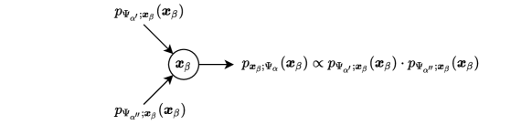
(a) Variable-to-factor message update.

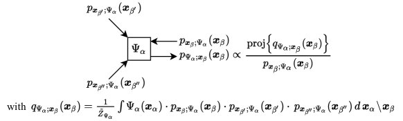
(b) Factor-to-variable message update.

Figure 4: Illustration of the EP message-passing update rules.

The approximate posterior distribution $\hat{p}_{\mathbf{x}_{\beta}}(\mathbf{x}_{\beta})$ of the variable $\mathbf{x}_{\beta}$ can be computed via [20]

$$\hat{p}_{\mathbf{x}_{\beta}}(\mathbf{x}_{\beta}) \propto\prod_{\alpha\in N_{\beta}}p_{\Psi_{\alpha};\mathbf{x}_{\beta}}(\mathbf{x}_{\beta}).$$ (72)

Appendix D Derivation of Message-Passing Update Rules for JACD-EP

In the following, we apply the EP message-passing rules presented in Appendix C to the factor graph in Fig. 1 and show the detailed derivations for the message updates. Here, the message updates are implicitly given by the computation of the corresponding probability distributions. Additionally, we use the properties of Gaussian distributions presented in Appendix B.

D-A Message Updates for Leaf Nodes $\Psi_{u_{k}}$, $\Psi_{h_{l,k}}$, and $\Psi_{x_{kt}}$

Since the prior distributions $\tilde{p}_{u_{k}}(u_{k})$, $\tilde{p}_{h_{l,k}}(\mathbf{h}_{l,k})$, and $p_{x}(x_{kt})$ are in the same exponential family as the approximate distributions of $u_{k}$, $\mathbf{h}_{l,k}$, and $x_{kt}$, respectively, the corresponding message updates simplify significantly. The factor-to-variable messages are constant and consist of the prior information on the variables $u_{k}$, $\mathbf{h}_{l,k}$, and $x_{kt}$ which correspond to the distributions

$$p_{\Psi_{u_{k}};u_{k}}(u_{k}) =\tilde{p}_{u_{k}}(u_{k}),$$ (73)

$$p_{\Psi_{h_{l,k}};\mathbf{h}_{l,k}}(\mathbf{h}_{l,k}) =\tilde{p}_{h_{l,k}}(\mathbf{h}_{l,k}),$$ (74)

$$p_{\Psi_{x_{kt}};x_{kt}}(x_{kt}) =p_{x}(x_{kt}).$$ (75)

This result is obtained by applying the message-passing rule in (69) while taking into account the fact that exponential family distributions are closed under multiplication. This makes the projection operation in (69) superfluous. Hence, the distributions corresponding to the updated messages are directly given by the factors $\Psi_{u_{k}}$, $\Psi_{h_{l,k}}$, and $\Psi_{x_{kt}}$, respectively, which correspond to the priors according to (9)-(11). The variable-to-factor messages for the leaf nodes are irrelevant in the unfolding of the algorithm and omitted here.

D-B Message Updates for $\Psi_{y_{l,t}}$

D-B1 Incoming messages to factor node $\Psi_{y_{l,t}}$

$$p_{\mathbf{z}_{l,kt};\Psi_{y_{l,t}}}(\mathbf{z}_{l,kt})=p_{\Psi_{z_{l,kt}};\mathbf{z}_{l,kt}}(\mathbf{z}_{l,kt}).$$ (76)

D-B2 Outgoing messages from factor node $\Psi_{y_{l,t}}$

Message Update $m_{\Psi_{y_{l,t}};\mathbf{z}_{l,kt}}$

$$p_{\Psi_{y_{l,t}};\mathbf{z}_{l,kt}}(\mathbf{z}_{l,kt})\propto\frac{\mathrm{proj}\!\left\{q_{\Psi_{y_{l,t}};\mathbf{z}_{l,kt}}(\mathbf{z}_{l,kt})\right\}}{p_{\mathbf{z}_{l,kt};\Psi_{y_{l,t}}}(\mathbf{z}_{l,kt})},$$ (77)

with

$$q_{\Psi_{y_{l,t}};\mathbf{z}_{l,kt}}(\mathbf{z}_{l,kt})$$

$$\quad\propto\int\!\!\cdots\!\!\int\mathcal{CN}\!\left(\mathbf{y}_{l,t}\Bigg{|}\sum_{k^{\prime}=1}^{K}\mathbf{z}_{l,k^{\prime}t},\sigma_{n}^{2}\mathbf{I}_{N}\right)\cdot p_{\mathbf{z}_{l,kt};\Psi_{y_{l,t}}}(\mathbf{z}_{l,kt})\cdot\prod_{k^{\prime}\neq k}p_{\mathbf{z}_{l,k^{\prime}t};\Psi_{y_{l,t}}}(\mathbf{z}_{l,k^{\prime}t})\,d\mathbf{z}_{l,k^{\prime}t}$$

$$\quad\overset{(a)}{=}\int\!\!\cdots\!\!\int\mathcal{CN}\!\left(\mathbf{z}_{l,k^{\prime\prime}t}\Bigg{|}\mathbf{y}_{l,t}-\sum_{k^{\prime}\neq k^{\prime\prime}}\mathbf{z}_{l,k^{\prime}t},\sigma_{n}^{2}\mathbf{I}_{N}\right)\cdot p_{\mathbf{z}_{l,kt};\Psi_{y_{l,t}}}(\mathbf{z}_{l,kt})$$

$$\qquad\qquad\quad\cdot\prod_{k^{\prime}\neq k}\mathcal{CN}\!\left(\mathbf{z}_{l,k^{\prime}t}\big{|}\boldsymbol{\mu}_{\Psi_{z_{l,k^{\prime}t}};\mathbf{z}_{l,k^{\prime}t}},\mathbf{C}_{\Psi_{z_{l,k^{\prime}t}};\mathbf{z}_{l,k^{\prime}t}}\right)\,d\mathbf{z}_{l,k^{\prime}t}$$

$$\quad\overset{(b)}{=}\int\!\!\cdots\!\!\int\mathcal{CN}\!\left(\mathbf{z}_{l,k^{\prime\prime}t}|\boldsymbol{\mu}_{\text{tmp}},\mathbf{C}_{\text{tmp}}\right)$$

$$\qquad\qquad\quad\cdot\mathcal{CN}\!\left(\mathbf{0}\Bigg{|}\mathbf{y}_{l,t}-\sum_{k^{\prime}\neq k^{\prime\prime}}\mathbf{z}_{l,k^{\prime}t}-\boldsymbol{\mu}_{\Psi_{z_{l,k^{\prime\prime}t}};\mathbf{z}_{l,k^{\prime\prime}t}},\sigma_{n}^{2}\mathbf{I}_{N}+\mathbf{C}_{\Psi_{z_{l,k^{\prime\prime}t}};\mathbf{z}_{l,k^{\prime\prime}t}}\right)\,d\mathbf{z}_{l,k^{\prime\prime}t}$$

$$\qquad\qquad\quad\cdot p_{\mathbf{z}_{l,kt};\Psi_{y_{l,t}}}(\mathbf{z}_{l,kt})\cdot\prod_{k^{\prime}\neq\{k,k^{\prime\prime}\}}\mathcal{CN}\!\left(\mathbf{z}_{l,k^{\prime}t}\big{|}\boldsymbol{\mu}_{\Psi_{z_{l,k^{\prime}t}};\mathbf{z}_{l,k^{\prime}t}},\mathbf{C}_{\Psi_{z_{l,k^{\prime}t}};\mathbf{z}_{l,k^{\prime}t}}\right)\,d\mathbf{z}_{l,k^{\prime}t}$$

$$\quad\overset{(c)}{=}\int\!\!\cdots\!\!\int\mathcal{CN}\!\left(\mathbf{y}_{l,t}\Bigg{|}\sum_{k^{\prime}\neq\{k^{\prime\prime}\}}\mathbf{z}_{l,k^{\prime}t}+\boldsymbol{\mu}_{\Psi_{z_{l,k^{\prime\prime}t}};\mathbf{z}_{l,k^{\prime\prime}t}},\sigma_{n}^{2}\mathbf{I}_{N}+\mathbf{C}_{\Psi_{z_{l,k^{\prime\prime}t}};\mathbf{z}_{l,k^{\prime\prime}t}}\right)$$

$$\qquad\qquad\quad\cdot p_{\mathbf{z}_{l,kt};\Psi_{y_{l,t}}}(\mathbf{z}_{l,kt})\cdot\prod_{k^{\prime}\neq\{k,k^{\prime\prime}\}}\mathcal{CN}\!\left(\mathbf{z}_{l,k^{\prime}t}\big{|}\boldsymbol{\mu}_{\Psi_{z_{l,k^{\prime}t}};\mathbf{z}_{l,k^{\prime}t}},\mathbf{C}_{\Psi_{z_{l,k^{\prime}t}};\mathbf{z}_{l,k^{\prime}t}}\right)\,d\mathbf{z}_{l,k^{\prime}t}$$

$$\quad=\dots$$

$$\quad=\mathcal{CN}\!\left(\mathbf{z}_{l,kt}\Big{|}\mathbf{y}_{l,t}-\sum_{k^{\prime}\neq k}\boldsymbol{\mu}_{\Psi_{z_{l,k^{\prime}t}};\mathbf{z}_{l,k^{\prime}t}},\sigma_{n}^{2}\mathbf{I}_{N}+\sum_{k^{\prime}\neq k}\mathbf{C}_{\Psi_{z_{l,k^{\prime}t}};\mathbf{z}_{l,k^{\prime}t}}\right)\cdot p_{\mathbf{z}_{l,kt};\Psi_{y_{l,t}}}(\mathbf{z}_{l,kt}),$$ (78)

where $(a)$ is obtained by a basic transformation of the Gaussian distribution and using (76), $(b)$ is obtained by the Gaussian product rule (61) with $\boldsymbol{\mu}_{1}=\mathbf{y}_{l,t}-\sum_{k^{\prime}\neq k^{\prime\prime}}\mathbf{z}_{l,k^{\prime}t}$, $\boldsymbol{\mu}_{2}=\boldsymbol{\mu}_{\Psi_{z_{l,k^{\prime\prime}t}};\mathbf{z}_{l,k^{\prime\prime}t}}$, $\mathbf{C}_{1}=\sigma_{n}^{2}\mathbf{I}_{N}$, and $\mathbf{C}_{2}=\mathbf{C}_{\Psi_{z_{l,k^{\prime\prime}t}};\mathbf{z}_{l,k^{\prime\prime}t}}$ which yields $\mathbf{C}_{\text{tmp}}$ and $\boldsymbol{\mu}_{\text{tmp}}$ according to (62) and (63), respectively, $(c)$ is obtained by integrating over $\mathbf{z}_{l,k^{\prime\prime}t}$ and applying a basic transformation of the Gaussian distribution, and the final equation (78) is obtained by repeatedly applying the above described steps for all $k^{\prime}\neq k$. Since $p_{\mathbf{z}_{l,kt};\Psi_{y_{l,t}}}(\mathbf{z}_{l,kt})$ is Gaussian distributed, we can conclude by utilizing the Gaussian product lemma that $q_{\Psi_{y_{l,t}};\mathbf{z}_{l,kt}}(\mathbf{z}_{l,kt})$ is Gaussian distributed as well. Hence, the projection operation in (77) is superfluous since it projects $q_{\Psi_{y_{l,t}};\mathbf{z}_{l,kt}}(\mathbf{z}_{l,kt})$ onto a Gaussian distribution which is the EP exponential family approximation choice of $\mathbf{z}_{l,kt}$. Therefore, the denominator of (77) cancels with the second term in (78), and the final message update rule is given by the distribution

$$p_{\Psi_{y_{l,t}};\mathbf{z}_{l,kt}}(\mathbf{z}_{l,kt})=\mathcal{CN}\!\left(\mathbf{z}_{l,kt}|\boldsymbol{\mu}_{\Psi_{y_{l,t}};\mathbf{z}_{l,kt}},\mathbf{C}_{\Psi_{y_{l,t}};\mathbf{z}_{l,kt}}\right),$$ (79)

with

$$\boldsymbol{\mu}_{\Psi_{y_{l,t}};\mathbf{z}_{l,kt}} =\mathbf{y}_{l,t}-\sum_{k^{\prime}\neq k}\boldsymbol{\mu}_{\Psi_{z_{l,k^{\prime}t}};\mathbf{z}_{l,k^{\prime}t}},$$ (80)

$$\mathbf{C}_{\Psi_{y_{l,t}};\mathbf{z}_{l,kt}} =\sigma_{n}^{2}\mathbf{I}_{N}+\sum_{k^{\prime}\neq k}\mathbf{C}_{\Psi_{z_{l,k^{\prime}t}};\mathbf{z}_{l,k^{\prime}t}}.$$ (81)

D-C Message Updates for $\Psi_{z_{l,kt}}$

D-C1 Incoming messages to factor node $\Psi_{z_{l,kt}}$

$$p_{x_{kt};\Psi_{z_{l,kt}}}(x_{kt}) \propto p_{\Psi_{x_{kt}};x_{kt}}(x_{kt})\cdot\prod_{l^{\prime}\neq l}p_{\Psi_{z_{l^{\prime},kt}};x_{kt}}(x_{kt}),$$ (82)

$$p_{\mathbf{z}_{l,kt};\Psi_{z_{l,kt}}}(\mathbf{z}_{l,kt}) =p_{\Psi_{y_{l,t}};\mathbf{z}_{l,kt}}(\mathbf{z}_{l,kt}),$$ (83)

$$p_{\mathbf{g}_{l,k};\Psi_{z_{l,kt}}}(\mathbf{g}_{l,k}) \propto p_{\Psi_{g_{l,k}};\mathbf{g}_{l,k}}(\mathbf{g}_{l,k})\cdot\prod_{t^{\prime}\neq t}p_{\Psi_{z_{l,kt^{\prime}}};\mathbf{g}_{l,k}}(\mathbf{g}_{l,k})$$

$$\propto\mathcal{CN}\!\left(\mathbf{g}_{l,k}|\boldsymbol{\mu}_{\mathbf{g}_{l,k};\Psi_{z_{l,kt}}},\mathbf{C}_{\mathbf{g}_{l,k};\Psi_{z_{l,kt}}}\right),$$ (84)

with

$$\mathbf{C}_{\mathbf{g}_{l,k};\Psi_{z_{l,kt}}} =\left(\mathbf{C}_{\Psi_{g_{l,k}};\mathbf{g}_{l,k}}^{-1}+\sum_{t^{\prime}\neq t}\mathbf{C}_{\Psi_{z_{l,kt^{\prime}}};\mathbf{g}_{l,k}}^{-1}\right)^{-1},$$ (85)

$$\boldsymbol{\mu}_{\mathbf{g}_{l,k};\Psi_{z_{l,kt}}} =\mathbf{C}_{\mathbf{g}_{l,k};\Psi_{z_{l,kt}}}\Bigg{(}\mathbf{C}_{\Psi_{g_{l,k}};\mathbf{g}_{l,k}}^{-1}\boldsymbol{\mu}_{\Psi_{g_{l,k}};\mathbf{g}_{l,k}}+\sum_{t^{\prime}\neq t}\mathbf{C}_{\Psi_{z_{l,kt^{\prime}}};\mathbf{g}_{l,k}}^{-1}\boldsymbol{\mu}_{\Psi_{z_{l,kt^{\prime}}};\mathbf{g}_{l,k}}\Bigg{)},$$ (86)

which is obtained by applying the Gaussian product lemma multiple times.

D-C2 Outgoing messages from factor node $\Psi_{z_{l,kt}}$

Message Update $m_{\Psi_{z_{l,kt}};x_{kt}}$

$$p_{\Psi_{z_{l,kt}};x_{kt}}(x_{kt})\propto\frac{\mathrm{proj}\!\left\{q_{\Psi_{z_{l,kt}};x_{kt}}(x_{kt})\right\}}{p_{x_{kt};\Psi_{z_{l,kt}}}(x_{kt})},$$ (87)

with

$$q_{\Psi_{z_{l,kt}};x_{kt}}(x_{kt}) \propto\int\int\delta(\mathbf{z}_{l,kt}-\mathbf{g}_{l,k}x_{kt})\cdot p_{x_{kt};\Psi_{z_{l,kt}}}(x_{kt})\cdot p_{\mathbf{z}_{l,kt};\Psi_{z_{l,kt}}}(\mathbf{z}_{l,kt})$$

$$\qquad\quad\cdot p_{\mathbf{g}_{l,k};\Psi_{z_{l,kt}}}(\mathbf{g}_{l,k})\,d\mathbf{z}_{l,kt}\,d\mathbf{g}_{l,k}$$

$$\overset{(a)}{=}\int p_{x_{kt};\Psi_{z_{l,kt}}}(x_{kt})\cdot p_{\mathbf{z}_{l,kt};\Psi_{z_{l,kt}}}(\mathbf{g}_{l,k}x_{kt})\cdot p_{\mathbf{g}_{l,k};\Psi_{z_{l,kt}}}(\mathbf{g}_{l,k})\,d\mathbf{g}_{l,k}$$

$$\overset{(b)}{=}\int p_{x_{kt};\Psi_{z_{l,kt}}}(x_{kt})\cdot\mathcal{CN}\!\left(\mathbf{g}_{l,k}x_{kt}|\boldsymbol{\mu}_{\Psi_{y_{l,t}};\mathbf{z}_{l,kt}},\mathbf{C}_{\Psi_{y_{l,t}};\mathbf{z}_{l,kt}}\right)$$

$$\qquad\cdot\mathcal{CN}\!\left(\mathbf{g}_{l,k}|\boldsymbol{\mu}_{\mathbf{g}_{l,k};\Psi_{z_{l,kt}}},\mathbf{C}_{\mathbf{g}_{l,k};\Psi_{z_{l,kt}}}\right)\,d\mathbf{g}_{l,k}$$

$$\overset{(c)}{=}\int p_{x_{kt};\Psi_{z_{l,kt}}}(x_{kt})\cdot|x_{kt}|^{-2N}\cdot\mathcal{CN}\!\left(\mathbf{g}_{l,k}|\boldsymbol{\mu}_{\text{tmp}},\mathbf{C}_{\text{tmp}}\right)$$

$$\qquad\cdot\mathcal{CN}\!\left(\mathbf{0}|\boldsymbol{\mu}_{\Psi_{y_{l,t}};\mathbf{z}_{l,kt}}x_{kt}^{-1}-\boldsymbol{\mu}_{\mathbf{g}_{l,k};\Psi_{z_{l,kt}}},\mathbf{C}_{\Psi_{y_{l,t}};\mathbf{z}_{l,kt}}|x_{kt}|^{-2}+\mathbf{C}_{\mathbf{g}_{l,k};\Psi_{z_{l,kt}}}\right)\,d\mathbf{g}_{l,k}$$

$$=p_{x_{kt};\Psi_{z_{l,kt}}}(x_{kt})\cdot|x_{kt}|^{-2N}$$

$$\quad\cdot\mathcal{CN}\!\left(\mathbf{0}|\boldsymbol{\mu}_{\Psi_{y_{l,t}};\mathbf{z}_{l,kt}}x_{kt}^{-1}-\boldsymbol{\mu}_{\mathbf{g}_{l,k};\Psi_{z_{l,kt}}},\mathbf{C}_{\Psi_{y_{l,t}};\mathbf{z}_{l,kt}}|x_{kt}|^{-2}+\mathbf{C}_{\mathbf{g}_{l,k};\Psi_{z_{l,kt}}}\right)$$

$$=p_{x_{kt};\Psi_{z_{l,kt}}}(x_{kt})\cdot\theta(x_{kt}),$$ (88)

where $(a)$ is obtained by the sifting property of the Dirac delta function [27], $(b)$ is obtained by using (83), $(c)$ is obtained by utilizing the Gaussian scaling lemma on $\mathcal{CN}\!\left(\mathbf{g}_{l,k}x_{kt}|\boldsymbol{\mu}_{\Psi_{y_{l,t}};\mathbf{z}_{l,kt}},\mathbf{C}_{\Psi_{y_{l,t}};\mathbf{z}_{l,kt}}\right)$ and then the Gaussian product lemma with $\boldsymbol{\mu}_{1}=\boldsymbol{\mu}_{\Psi_{y_{l,t}};\mathbf{z}_{l,kt}}x_{kt}^{-1}$, $\boldsymbol{\mu}_{2}=\boldsymbol{\mu}_{\mathbf{g}_{l,k};\Psi_{z_{l,kt}}}$, $\mathbf{C}_{1}=\mathbf{C}_{\Psi_{y_{l,t}};\mathbf{z}_{l,kt}}|x_{kt}|^{-2}$, and $\mathbf{C}_{2}=\mathbf{C}_{\mathbf{g}_{l,k};\Psi_{z_{l,kt}}}$ which yields $\mathbf{C}_{\text{tmp}}$ and $\boldsymbol{\mu}_{\text{tmp}}$ according to (62) and (63), respectively, and the final equation (88) is obtained by applying the Gaussian scaling lemma once again with

$$\theta(x_{kt})=\mathcal{CN}\!\left(\mathbf{0}|\boldsymbol{\mu}_{\Psi_{y_{l,t}};\mathbf{z}_{l,kt}}-\boldsymbol{\mu}_{\mathbf{g}_{l,k};\Psi_{z_{l,kt}}}x_{kt},\mathbf{C}_{\Psi_{y_{l,t}};\mathbf{z}_{l,kt}}+\mathbf{C}_{\mathbf{g}_{l,k};\Psi_{z_{l,kt}}}|x_{kt}|^{2}\right).$$ (89)

Evaluating (88) at $x_{kt}\in\mathcal{X}$ for $t>T_{p}$ yields a categorical distribution for $q_{\Psi_{z_{l,kt}};x_{kt}}(x_{kt})$. Hence, the projection operation in (87) is superfluous since it projects $q_{\Psi_{z_{l,kt}};x_{kt}}(x_{kt})$ onto a categorical distribution, and the denominator of (87) cancels with the first term in (88). Thus, the final message update rule is given by the distribution

$$p_{\Psi_{z_{l,kt}};x_{kt}}(x_{kt})\propto\theta(x_{kt}).$$ (90)

Message Update $m_{\Psi_{z_{l,kt}};\mathbf{z}_{l,kt}}$

$$p_{\Psi_{z_{l,kt}};\mathbf{z}_{l,kt}}(\mathbf{z}_{l,kt})\propto\frac{\mathrm{proj}\!\left\{q_{\Psi_{z_{l,kt}};\mathbf{z}_{l,kt}}(\mathbf{z}_{l,kt})\right\}}{p_{\mathbf{z}_{l,kt};\Psi_{z_{l,kt}}}(\mathbf{z}_{l,kt})},$$ (91)

with

$$q_{\Psi_{z_{l,kt}};\mathbf{z}_{l,kt}}(\mathbf{z}_{l,kt})$$

$$\quad\propto\sum_{x_{kt}}\int\delta(\mathbf{z}_{l,kt}-\mathbf{g}_{l,k}x_{kt})\cdot p_{x_{kt};\Psi_{z_{l,kt}}}(x_{kt})\cdot p_{\mathbf{z}_{l,kt};\Psi_{z_{l,kt}}}(\mathbf{z}_{l,kt})\cdot p_{\mathbf{g}_{l,k};\Psi_{z_{l,kt}}}(\mathbf{g}_{l,k})\,d\mathbf{g}_{l,k}$$

$$\quad\overset{(a)}{=}\sum_{x_{kt}}|x_{kt}|^{-2N}\cdot p_{x_{kt};\Psi_{z_{l,kt}}}(x_{kt})\cdot p_{\Psi_{y_{l,t}};\mathbf{z}_{l,kt}}(\mathbf{z}_{l,kt})\cdot p_{\mathbf{g}_{l,k};\Psi_{z_{l,kt}}}\left(\frac{\mathbf{z}_{l,kt}}{x_{kt}}\right)$$

$$\quad=\sum_{x_{kt}}p_{x_{kt};\Psi_{z_{l,kt}}}(x_{kt})\cdot\mathcal{CN}\!\left(\mathbf{z}_{l,kt}|\check{\boldsymbol{\mu}}_{\Psi_{z_{l,kt}};\mathbf{z}_{l,kt}}(x_{kt}),\check{\mathbf{C}}_{\Psi_{z_{l,kt}};\mathbf{z}_{l,kt}}(x_{kt})\right)\cdot\theta(x_{kt}),$$ (92)

where $(a)$ is obtained by applying the scaling and sifting property of the Dirac delta function [27] and the final equation (92) is obtained by the Gaussian scaling and product lemma with $\theta(x_{kt})$ given in (89) and

$$\check{\mathbf{C}}_{\Psi_{z_{l,kt}};\mathbf{z}_{l,kt}}(x_{kt}) =\left(\mathbf{C}_{\Psi_{y_{l,t}};\mathbf{z}_{l,kt}}^{-1}+\mathbf{C}_{\mathbf{g}_{l,k};\Psi_{z_{l,kt}}}^{-1}|x_{kt}|^{-2}\right)^{-1},$$ (93)

$$\check{\boldsymbol{\mu}}_{\Psi_{z_{l,kt}};\mathbf{z}_{l,kt}}(x_{kt}) =\check{\mathbf{C}}_{\Psi_{z_{l,kt}};\mathbf{z}_{l,kt}}(x_{kt})\Bigg{(}\mathbf{C}_{\Psi_{y_{l,t}};\mathbf{z}_{l,kt}}^{-1}\boldsymbol{\mu}_{\Psi_{y_{l,t}};\mathbf{z}_{l,kt}}+\mathbf{C}_{\mathbf{g}_{l,k};\Psi_{z_{l,kt}}}^{-1}\boldsymbol{\mu}_{\mathbf{g}_{l,k};\Psi_{z_{l,kt}}}\frac{x_{kt}}{|x_{kt}|^{2}}\Bigg{)}.$$ (94)

The normalization constant for $q_{\Psi_{z_{l,kt}};\mathbf{z}_{l,kt}}(\mathbf{z}_{l,kt})$ is given by

$$\tilde{Z}_{\Psi_{z_{l,kt}}} =\int\sum_{x_{kt}}p_{x_{kt};\Psi_{z_{l,kt}}}(x_{kt})\cdot\mathcal{CN}\!\left(\mathbf{z}_{l,kt}|\check{\boldsymbol{\mu}}_{\Psi_{z_{l,kt}};\mathbf{z}_{l,kt}}(x_{kt}),\check{\mathbf{C}}_{\Psi_{z_{l,kt}};\mathbf{z}_{l,kt}}(x_{kt})\right)\cdot\theta(x_{kt})\,d\mathbf{z}_{l,kt}$$

$$=\sum_{x_{kt}}p_{x_{kt};\Psi_{z_{l,kt}}}(x_{kt})\cdot\theta(x_{kt})$$ (95)

According to (92), $q_{\Psi_{z_{l,kt}};\mathbf{z}_{l,kt}}(\mathbf{z}_{l,kt})$ is a Gaussian mixture with mean vector and covariance matrix

$$\hat{\boldsymbol{\mu}}_{\Psi_{z_{l,kt}};\mathbf{z}_{l,kt}} =\frac{1}{\tilde{Z}_{\Psi_{z_{l,kt}}}}\sum_{x_{kt}}p_{x_{kt};\Psi_{z_{l,kt}}}(x_{kt})\cdot\theta(x_{kt})\cdot\check{\boldsymbol{\mu}}_{\Psi_{z_{l,kt}};\mathbf{z}_{l,kt}}(x_{kt}),$$ (96)

$$\begin{split}\hat{\mathbf{C}}_{\Psi_{z_{l,kt}};\mathbf{z}_{l,kt}}&=\frac{1}{\tilde{Z}_{\Psi_{z_{l,kt}}}}\sum_{x_{kt}}p_{x_{kt};\Psi_{z_{l,kt}}}(x_{kt})\cdot\theta(x_{kt})\cdot\Big{(}\check{\mathbf{C}}_{\Psi_{z_{l,kt}};\mathbf{z}_{l,kt}}(x_{kt})\\ &\quad+\check{\boldsymbol{\mu}}_{\Psi_{z_{l,kt}};\mathbf{z}_{l,kt}}(x_{kt})\check{\boldsymbol{\mu}}_{\Psi_{z_{l,kt}};\mathbf{z}_{l,kt}}^{H}(x_{kt})\Big{)}-\hat{\boldsymbol{\mu}}_{\Psi_{z_{l,kt}};\mathbf{z}_{l,kt}}\hat{\boldsymbol{\mu}}_{\Psi_{z_{l,kt}};\mathbf{z}_{l,kt}}^{H}.\end{split}$$ (97)

Note that in the pilot phase for $t<T_{p}$, the transmitted symbol $x_{kt}$ is already known. Hence, $q_{\Psi_{z_{l,kt}};\mathbf{z}_{l,kt}}(\mathbf{z}_{l,kt})$ reduces to a Gaussian distribution for $t<T_{p}$ with mean vector $\hat{\boldsymbol{\mu}}_{\Psi_{z_{l,kt}};\mathbf{z}_{l,kt}}=\check{\boldsymbol{\mu}}_{\Psi_{z_{l,kt}};\mathbf{z}_{l,kt}}$ and covariance matrix $\hat{\mathbf{C}}_{\Psi_{z_{l,kt}};\mathbf{z}_{l,kt}}=\check{\mathbf{C}}_{\Psi_{z_{l,kt}};\mathbf{z}_{l,kt}}$. The final message update can be computed according to (91) using moment matching to find the projected distribution and the Gaussian quotient lemma,

$$p_{\Psi_{z_{l,kt}};\mathbf{z}_{l,kt}}(\mathbf{z}_{l,kt})=\mathcal{CN}\!\left(\mathbf{z}_{l,kt}|\boldsymbol{\mu}_{\Psi_{z_{l,kt}};\mathbf{z}_{l,kt}},\mathbf{C}_{\Psi_{z_{l,kt}};\mathbf{z}_{l,kt}}\right),$$ (98)

with

$$\mathbf{C}_{\Psi_{z_{l,kt}};\mathbf{z}_{l,kt}} =\left(\hat{\mathbf{C}}_{\Psi_{z_{l,kt}};\mathbf{z}_{l,kt}}^{-1}-\mathbf{C}_{\Psi_{y_{l,t}};\mathbf{z}_{l,kt}}^{-1}\right)^{-1},$$ (99)

$$\boldsymbol{\mu}_{\Psi_{z_{l,kt}};\mathbf{z}_{l,kt}} =\mathbf{C}_{\Psi_{z_{l,kt}};\mathbf{z}_{l,kt}}\left(\hat{\mathbf{C}}_{\Psi_{z_{l,kt}};\mathbf{z}_{l,kt}}^{-1}\hat{\boldsymbol{\mu}}_{\Psi_{z_{l,kt}};\mathbf{z}_{l,kt}}-\mathbf{C}_{\Psi_{y_{l,t}};\mathbf{z}_{l,kt}}^{-1}\boldsymbol{\mu}_{\Psi_{y_{l,t}};\mathbf{z}_{l,kt}}\right).$$ (100)

Message Update $m_{\Psi_{z_{l,kt}};\mathbf{g}_{l,k}}$

$$p_{\Psi_{z_{l,kt}};\mathbf{g}_{l,k}}(\mathbf{g}_{l,k})\propto\frac{\mathrm{proj}\!\left\{q_{\Psi_{z_{l,kt}};\mathbf{g}_{l,k}}(\mathbf{g}_{l,k})\right\}}{p_{\mathbf{g}_{l,k};\Psi_{z_{l,kt}}}(\mathbf{g}_{l,k})},$$ (101)

with

$$q_{\Psi_{z_{l,kt}};\mathbf{g}_{l,k}}(\mathbf{g}_{l,k})$$

$$\quad\propto\sum_{x_{kt}}\int\delta(\mathbf{z}_{l,kt}-\mathbf{g}_{l,k}x_{kt})\cdot p_{x_{kt};\Psi_{z_{l,kt}}}(x_{kt})\cdot p_{\mathbf{z}_{l,kt};\Psi_{z_{l,kt}}}(\mathbf{z}_{l,kt})\cdot p_{\mathbf{g}_{l,k};\Psi_{z_{l,kt}}}(\mathbf{g}_{l,k})\,d\mathbf{z}_{l,kt}$$

$$\quad\overset{(a)}{=}\sum_{x_{kt}}p_{x_{kt};\Psi_{z_{l,kt}}}(x_{kt})\cdot p_{\Psi_{y_{l,t}};\mathbf{z}_{l,kt}}(\mathbf{g}_{l,k}x_{kt})\cdot p_{\mathbf{g}_{l,k};\Psi_{z_{l,kt}}}(\mathbf{g}_{l,k})$$

$$\quad=\sum_{x_{kt}}p_{x_{kt};\Psi_{z_{l,kt}}}(x_{kt})\cdot\mathcal{CN}\!\left(\mathbf{g}_{l,k}|\check{\boldsymbol{\mu}}_{\Psi_{z_{l,kt}};\mathbf{g}_{l,k}}(x_{kt}),\check{\mathbf{C}}_{\Psi_{z_{l,kt}};\mathbf{g}_{l,k}}(x_{kt})\right)\cdot\theta(x_{kt}),$$ (102)

where $(a)$ is obtained by the sifting property of the Dirac delta function and the final equation (102) is obtained by the Gaussian scaling and product lemma with $\theta$ given in (89) and

$$\check{\mathbf{C}}_{\Psi_{z_{l,kt}};\mathbf{g}_{l,k}}(x_{kt}) =\left(\mathbf{C}_{\Psi_{y_{l,t}};\mathbf{z}_{l,kt}}^{-1}|x_{kt}|^{2}+\mathbf{C}_{\mathbf{g}_{l,k};\Psi_{z_{l,kt}}}^{-1}\right)^{-1},$$ (103)

$$\check{\boldsymbol{\mu}}_{\Psi_{z_{l,kt}};\mathbf{g}_{l,k}}(x_{kt}) =\check{\mathbf{C}}_{\Psi_{z_{l,kt}};\mathbf{g}_{l,k}}(x_{kt})\Bigg{(}\mathbf{C}_{\Psi_{y_{l,t}};\mathbf{z}_{l,kt}}^{-1}\boldsymbol{\mu}_{\Psi_{y_{l,t}};\mathbf{z}_{l,kt}}\frac{|x_{kt}|^{2}}{x_{kt}}+\mathbf{C}_{\mathbf{g}_{l,k};\Psi_{z_{l,kt}}}^{-1}\boldsymbol{\mu}_{\mathbf{g}_{l,k};\Psi_{z_{l,kt}}}\Bigg{)},$$ (104)

According to (102), $q_{\Psi_{z_{l,kt}};\mathbf{g}_{l,k}}(\mathbf{g}_{l,k})$ is a Gaussian mixture with mean vector and covariance matrix

$$\hat{\boldsymbol{\mu}}_{\Psi_{z_{l,kt}};\mathbf{g}_{l,k}} =\frac{1}{\tilde{Z}_{\Psi_{z_{l,kt}}}}\sum_{x_{kt}}p_{x_{kt};\Psi_{z_{l,kt}}}(x_{kt})\cdot\theta(x_{kt})\cdot\check{\boldsymbol{\mu}}_{\Psi_{z_{l,kt}};\mathbf{g}_{l,k}}(x_{kt}),$$ (105)

$$\begin{split}\hat{\mathbf{C}}_{\Psi_{z_{l,kt}};\mathbf{g}_{l,k}}&=\frac{1}{\tilde{Z}_{\Psi_{z_{l,kt}}}}\sum_{x_{kt}}p_{x_{kt};\Psi_{z_{l,kt}}}(x_{kt})\cdot\theta(x_{kt})\cdot\Big{(}\check{\mathbf{C}}_{\Psi_{z_{l,kt}};\mathbf{g}_{l,k}}(x_{kt})\\ &\quad+\check{\boldsymbol{\mu}}_{\Psi_{z_{l,kt}};\mathbf{g}_{l,k}}(x_{kt})\check{\boldsymbol{\mu}}_{\Psi_{z_{l,kt}};\mathbf{g}_{l,k}}^{H}(x_{kt})\Big{)}-\hat{\boldsymbol{\mu}}_{\Psi_{z_{l,kt}};\mathbf{g}_{l,k}}\hat{\boldsymbol{\mu}}_{\Psi_{z_{l,kt}};\mathbf{g}_{l,k}}^{H}.\end{split}$$ (106)

Note that in the pilot phase for $t<T_{p}$, the transmitted symbol $x_{kt}$ is already known. Hence, $q_{\Psi_{z_{l,kt}};\mathbf{g}_{l,k}}(\mathbf{g}_{l,k})$ reduces to a Gaussian distribution for $t<T_{p}$ with mean vector $\hat{\boldsymbol{\mu}}_{\Psi_{z_{l,kt}};\mathbf{g}_{l,k}}=\check{\boldsymbol{\mu}}_{\Psi_{z_{l,kt}};\mathbf{g}_{l,k}}$ and covariance matrix $\hat{\mathbf{C}}_{\Psi_{z_{l,kt}};\mathbf{g}_{l,k}}=\check{\mathbf{C}}_{\Psi_{z_{l,kt}};\mathbf{g}_{l,k}}$. The final message update can be computed according to (101) using moment matching and the Gaussian quotient lemma,

$$p_{\Psi_{z_{l,kt}};\mathbf{g}_{l,k}}(\mathbf{g}_{l,k})=\mathcal{CN}\!\left(\mathbf{g}_{l,k}|\boldsymbol{\mu}_{\Psi_{z_{l,kt}};\mathbf{g}_{l,k}},\mathbf{C}_{\Psi_{z_{l,kt}};\mathbf{g}_{l,k}}\right),$$ (107)

with

$$\mathbf{C}_{\Psi_{z_{l,kt}};\mathbf{g}_{l,k}} =\left(\hat{\mathbf{C}}_{\Psi_{z_{l,kt}};\mathbf{g}_{l,k}}^{-1}-\mathbf{C}_{\mathbf{g}_{l,k};\Psi_{z_{l,kt}}}^{-1}\right)^{-1},$$ (108)

$$\boldsymbol{\mu}_{\Psi_{z_{l,kt}};\mathbf{g}_{l,k}} =\mathbf{C}_{\Psi_{z_{l,kt}};\mathbf{g}_{l,k}}\left(\hat{\mathbf{C}}_{\Psi_{z_{l,kt}};\mathbf{g}_{l,k}}^{-1}\hat{\boldsymbol{\mu}}_{\Psi_{z_{l,kt}};\mathbf{g}_{l,k}}-\mathbf{C}_{\mathbf{g}_{l,k};\Psi_{z_{l,kt}}}^{-1}\boldsymbol{\mu}_{\mathbf{g}_{l,k};\Psi_{z_{l,kt}}}\right).$$ (109)

D-D Message Updates for $\Psi_{g_{l,k}}$

D-D1 Incoming messages to factor node $\Psi_{g_{l,k}}$

$$p_{u_{k};\Psi_{g_{l,k}}}(u_{k}) \propto p_{\Psi_{u_{k}};u_{k}}(u_{k})\cdot\prod_{l^{\prime}\neq l}p_{\Psi_{g_{l^{\prime},k}};u_{k}}(u_{k}),$$ (110)

$$p_{\mathbf{h}_{l,k};\Psi_{g_{l,k}}}(\mathbf{h}_{l,k}) =p_{\Psi_{h_{l,k}};\mathbf{h}_{l,k}}(\mathbf{h}_{l,k}),$$ (111)

$$p_{\mathbf{g}_{l,k};\Psi_{g_{l,k}}}(\mathbf{g}_{l,k}) \propto\prod_{t=1}^{T}p_{\Psi_{z_{l,kt}};\mathbf{g}_{l,k}}(\mathbf{g}_{l,k})$$

$$\propto\mathcal{CN}\!\left(\mathbf{g}_{l,k}|\boldsymbol{\mu}_{\mathbf{g}_{l,k};\Psi_{g_{l,k}}},\mathbf{C}_{\mathbf{g}_{l,k};\Psi_{g_{l,k}}}\right),$$ (112)

with

$$\mathbf{C}_{\mathbf{g}_{l,k};\Psi_{g_{l,k}}} =\left(\sum_{t=1}^{T}\mathbf{C}_{\Psi_{z_{l,kt}};\mathbf{g}_{l,k}}^{-1}\right)^{-1},$$ (113)

$$\boldsymbol{\mu}_{\mathbf{g}_{l,k};\Psi_{g_{l,k}}} =\mathbf{C}_{\mathbf{g}_{l,k};\Psi_{g_{l,k}}}\left(\sum_{t=1}^{T}\mathbf{C}_{\Psi_{z_{l,kt}};\mathbf{g}_{l,k}}^{-1}\boldsymbol{\mu}_{\Psi_{z_{l,kt}};\mathbf{g}_{l,k}}\right),$$ (114)

which is obtained by applying the Gaussian product lemma multiple times.

D-D2 Outgoing messages from factor node $\Psi_{g_{l,k}}$

Message Update $m_{\Psi_{g_{l,k}};u_{k}}$

$$p_{\Psi_{g_{l,k}};u_{k}}(u_{k})\propto\frac{\mathrm{proj}\!\left\{q_{\Psi_{g_{l,k}};u_{k}}(u_{k})\right\}}{p_{u_{k};\Psi_{g_{l,k}}}(u_{k})},$$ (115)

with

$$q_{\Psi_{g_{l,k}};u_{k}}(u_{k}) \propto\int\int\delta(\mathbf{g}_{l,k}-\mathbf{h}_{l,k}u_{k})\cdot p_{u_{k};\Psi_{g_{l,k}}}(u_{k})\cdot p_{\mathbf{g}_{l,k};\Psi_{g_{l,k}}}(\mathbf{g}_{l,k})\cdot p_{\mathbf{h}_{l,k};\Psi_{g_{l,k}}}(\mathbf{h}_{l,k})\,d\mathbf{g}_{l,k}\,d\mathbf{h}_{l,k}$$

$$\overset{(a)}{=}\int p_{u_{k};\Psi_{g_{l,k}}}(u_{k})\cdot p_{\mathbf{g}_{l,k};\Psi_{g_{l,k}}}(\mathbf{h}_{l,k}u_{k})\cdot p_{\Psi_{h_{l,k}};\mathbf{h}_{l,k}}(\mathbf{h}_{l,k})\,d\mathbf{h}_{l,k}$$

$$=p_{u_{k};\Psi_{g_{l,k}}}(u_{k})\cdot\vartheta(u_{k}),$$ (116)

where $(a)$ is obtained by the sifting property of the Dirac delta function and the final equation (116) is obtained by considering the fact that $u_{k}$ is a binary random variable with $u_{k}\in\{0,1\}$, utilizing (74) and the Gaussian product rule, and, then, integrating over $\mathbf{h}_{l,k}$ with

$$\vartheta(u_{k})=\mathcal{CN}\!\left(\mathbf{0}|\boldsymbol{\mu}_{\mathbf{g}_{l,k};\Psi_{g_{l,k}}}-\tilde{\boldsymbol{\mu}}_{h_{l,k}}u_{k},\mathbf{C}_{\mathbf{g}_{l,k};\Psi_{g_{l,k}}}+\tilde{\mathbf{C}}_{h_{l,k}}u_{k}\right).$$ (117)

The projection operation in (115) is superfluous since $q_{\Psi_{g_{l,k}};u_{k}}(u_{k})$ (116) is already categorically distributed. Hence, the denominator of (115) cancels with the first term in (116). The final message update rule is given by the distribution

$$p_{\Psi_{g_{l,k}};u_{k}}(u_{k})\propto\vartheta(u_{k}).$$ (118)

Message Update $m_{\Psi_{g_{l,k}};\mathbf{h}_{l,k}}$

$$p_{\Psi_{g_{l,k}};\mathbf{h}_{l,k}}(\mathbf{h}_{l,k})\propto\frac{\mathrm{proj}\!\left\{q_{\Psi_{g_{l,k}};\mathbf{h}_{l,k}}(\mathbf{h}_{l,k})\right\}}{p_{\mathbf{h}_{l,k};\Psi_{g_{l,k}}}(\mathbf{h}_{l,kt})},$$ (119)

with

$$q_{\Psi_{g_{l,k}};\mathbf{h}_{l,k}}(\mathbf{h}_{l,k}) \propto\sum_{u_{k}}\int\delta(\mathbf{g}_{l,k}-\mathbf{h}_{l,k}u_{k})\cdot p_{u_{k};\Psi_{g_{l,k}}}(u_{k})\cdot p_{\mathbf{g}_{l,k};\Psi_{g_{l,k}}}(\mathbf{g}_{l,k})\cdot p_{\mathbf{h}_{l,k};\Psi_{g_{l,k}}}(\mathbf{h}_{l,k})\,d\mathbf{g}_{l,k}$$

$$\overset{(a)}{=}p_{u_{k};\Psi_{g_{l,k}}}(0)\cdot p_{\mathbf{g}_{l,k};\Psi_{g_{l,k}}}(\mathbf{0})\cdot p_{\Psi_{h_{l,k}};\mathbf{h}_{l,k}}(\mathbf{h}_{l,k})+p_{u_{k};\Psi_{g_{l,k}}}(1)\cdot p_{\mathbf{g}_{l,k};\Psi_{g_{l,k}}}(\mathbf{h}_{l,k})$$

$$\quad\cdot p_{\Psi_{h_{l,k}};\mathbf{h}_{l,k}}(\mathbf{h}_{l,k})$$

$$\begin{split}&=p_{u_{k};\Psi_{g_{l,k}}}(0)\cdot\vartheta(0)\cdot p_{\Psi_{h_{l,k}};\mathbf{h}_{l,k}}(\mathbf{h}_{l,k})+p_{u_{k};\Psi_{g_{l,k}}}(1)\cdot\vartheta(1)\\ &\quad\cdot\mathcal{CN}\!\left(\mathbf{h}_{l,k}|\check{\boldsymbol{\mu}}_{\Psi_{g_{l,k}};\mathbf{h}_{l,k}},\check{\mathbf{C}}_{\Psi_{g_{l,k}};\mathbf{h}_{l,k}}\right),\end{split}$$ (120)

where $(a)$ is obtained by writing out the sum over $u_{k}$ and utilizing the sifting property of the Dirac delta function, and the final equation (120) is obtained by using (74), (117), and the Gaussian multiplication lemma with

$$\check{\mathbf{C}}_{\Psi_{g_{l,k}};\mathbf{h}_{l,k}} =\left(\mathbf{C}_{\mathbf{g}_{l,k};\Psi_{g_{l,k}}}^{-1}+\tilde{\mathbf{C}}_{h_{l,k}}^{-1}\right)^{-1},$$ (121)

$$\check{\boldsymbol{\mu}}_{\Psi_{g_{l,k}};\mathbf{h}_{l,k}} =\check{\mathbf{C}}_{\Psi_{g_{l,k}};\mathbf{h}_{l,k}}\Bigg{(}\mathbf{C}_{\mathbf{g}_{l,k};\Psi_{g_{l,k}}}^{-1}\boldsymbol{\mu}_{\mathbf{g}_{l,k};\Psi_{g_{l,k}}}+\tilde{\mathbf{C}}_{h_{l,k}}^{-1}\tilde{\boldsymbol{\mu}}_{h_{l,k}}\Bigg{)}.$$ (122)

The normalization constant for $q_{\Psi_{g_{l,k}};\mathbf{h}_{l,k}}(\mathbf{h}_{l,k})$ is given by

$$\tilde{Z}_{\Psi_{g_{l,k}}} =\int p_{u_{k};\Psi_{g_{l,k}}}(0)\cdot\vartheta(0)\cdot p_{\Psi_{h_{l,k}};\mathbf{h}_{l,k}}(\mathbf{h}_{l,k})$$

$$\qquad+p_{u_{k};\Psi_{g_{l,k}}}(1)\cdot\vartheta(1)\cdot\mathcal{CN}\!\left(\mathbf{h}_{l,k}|\check{\boldsymbol{\mu}}_{\Psi_{g_{l,k}};\mathbf{h}_{l,k}},\check{\mathbf{C}}_{\Psi_{g_{l,k}};\mathbf{h}_{l,k}}\right)\,d\mathbf{h}_{l,k}$$

$$=p_{u_{k};\Psi_{g_{l,k}}}(0)\cdot\vartheta(0)+p_{u_{k};\Psi_{g_{l,k}}}(1)\cdot\vartheta(1).$$ (123)

According to (120), $q_{\Psi_{g_{l,k}};\mathbf{h}_{l,k}}(\mathbf{h}_{l,k})$ is a Gaussian mixture in two components with mean vector and covariance matrix

$$\hat{\boldsymbol{\mu}}_{\Psi_{g_{l,k}};\mathbf{h}_{l,k}} =\frac{1}{\tilde{Z}_{\Psi_{g_{l,k}}}}\Big{(}p_{u_{k};\Psi_{g_{l,k}}}(0)\cdot\vartheta(0)\cdot\tilde{\boldsymbol{\mu}}_{h_{l,k}}+p_{u_{k};\Psi_{g_{l,k}}}(1)\cdot\vartheta(1)\cdot\check{\boldsymbol{\mu}}_{\Psi_{g_{l,k}};\mathbf{h}_{l,k}}\Big{)},$$ (124)

$$\begin{split}\hat{\mathbf{C}}_{\Psi_{g_{l,k}};\mathbf{h}_{l,k}}&=\frac{1}{\tilde{Z}_{\Psi_{z_{l,kt}}}}\Big{(}p_{u_{k};\Psi_{g_{l,k}}}(0)\cdot\vartheta(0)\cdot\big{(}\tilde{\mathbf{C}}_{h_{l,k}}+\tilde{\boldsymbol{\mu}}_{h_{l,k}}\tilde{\boldsymbol{\mu}}_{h_{l,k}}^{H}\big{)}+p_{u_{k};\Psi_{g_{l,k}}}(1)\cdot\vartheta(1)\\ &\qquad\qquad\quad\cdot\big{(}\check{\mathbf{C}}_{\Psi_{g_{l,k}};\mathbf{h}_{l,k}}+\check{\boldsymbol{\mu}}_{\Psi_{g_{l,k}};\mathbf{h}_{l,k}}\check{\boldsymbol{\mu}}_{\Psi_{g_{l,k}};\mathbf{h}_{l,k}}^{H}\big{)}\Big{)}-\hat{\boldsymbol{\mu}}_{\Psi_{g_{l,k}};\mathbf{g}_{l,k}}\hat{\boldsymbol{\mu}}_{\Psi_{g_{l,k}};\mathbf{g}_{l,k}}^{H}.\end{split}$$ (125)

Note that the estimated posterior distribution (72) of $\mathbf{h}_{l,k}$ is proportional to the product of $p_{\Psi_{g_{l,k}};\mathbf{h}_{l,k}}(\mathbf{h}_{l,k})$ and $p_{\Psi_{h_{l,k}};\mathbf{h}_{l,k}}(\mathbf{h}_{l,kt})$ which is proportional to $\mathrm{proj}\!\left\{q_{\Psi_{g_{l,k}};\mathbf{h}_{l,k}}(\mathbf{h}_{l,k})\right\}$ according to (111) and (119). Hence, the final estimate of $\mathbf{h}_{l,k}$ can be computed via (124) after the last iteration of the EP algorithm.

Using moment matching and the Gaussian quotient lemma, the final message update can be computed according to (119) with the distribution

$$p_{\Psi_{g_{l,k}};\mathbf{h}_{l,k}}(\mathbf{h}_{l,k})=\mathcal{CN}\!\left(\mathbf{h}_{l,k}|\boldsymbol{\mu}_{\Psi_{g_{l,k}};\mathbf{h}_{l,k}},\mathbf{C}_{\Psi_{g_{l,k}};\mathbf{h}_{l,k}}\right),$$ (126)

with

$$\mathbf{C}_{\Psi_{g_{l,k}};\mathbf{h}_{l,k}} =\left(\hat{\mathbf{C}}_{\Psi_{g_{l,k}};\mathbf{h}_{l,k}}^{-1}-\tilde{\mathbf{C}}_{h_{l,k}}^{-1}\right)^{-1},$$ (127)

$$\boldsymbol{\mu}_{\Psi_{g_{l,k}};\mathbf{h}_{l,k}} =\mathbf{C}_{\Psi_{g_{l,k}};\mathbf{h}_{l,k}}\left(\hat{\mathbf{C}}_{\Psi_{g_{l,k}};\mathbf{h}_{l,k}}^{-1}\hat{\boldsymbol{\mu}}_{\Psi_{g_{l,k}};\mathbf{h}_{l,k}}-\tilde{\mathbf{C}}_{h_{l,k}}^{-1}\tilde{\boldsymbol{\mu}}_{h_{l,k}}\right).$$ (128)

Message Update $m_{\Psi_{g_{l,k}};\mathbf{g}_{l,k}}$

$$p_{\Psi_{g_{l,k}};\mathbf{g}_{l,k}}(\mathbf{g}_{l,k})\propto\frac{\mathrm{proj}\!\left\{q_{\Psi_{g_{l,k}};\mathbf{g}_{l,k}}(\mathbf{g}_{l,k})\right\}}{p_{\mathbf{g}_{l,k};\Psi_{g_{l,k}}}(\mathbf{g}_{l,kt})},$$ (129)

with

$$q_{\Psi_{g_{l,k}};\mathbf{g}_{l,k}}(\mathbf{g}_{l,k}) \propto\sum_{u_{k}}\int\delta(\mathbf{g}_{l,k}-\mathbf{h}_{l,k}u_{k})\cdot p_{u_{k};\Psi_{g_{l,k}}}(u_{k})\cdot p_{\mathbf{g}_{l,k};\Psi_{g_{l,k}}}(\mathbf{g}_{l,k})\cdot p_{\mathbf{h}_{l,k};\Psi_{g_{l,k}}}(\mathbf{h}_{l,k})\,d\mathbf{h}_{l,k}$$

$$\overset{(a)}{=}p_{u_{k};\Psi_{g_{l,k}}}(0)\cdot p_{\mathbf{g}_{l,k};\Psi_{g_{l,k}}}(\mathbf{g}_{l,k})\cdot\delta(\mathbf{g}_{l,k})+p_{u_{k};\Psi_{g_{l,k}}}(1)\cdot p_{\mathbf{g}_{l,k};\Psi_{g_{l,k}}}(\mathbf{g}_{l,k})$$

$$\quad\cdot p_{\Psi_{h_{l,k}};\mathbf{h}_{l,k}}(\mathbf{g}_{l,k})$$

$$\begin{split}&=p_{u_{k};\Psi_{g_{l,k}}}(0)\cdot p_{\mathbf{g}_{l,k};\Psi_{g_{l,k}}}(\mathbf{g}_{l,k})\cdot\delta(\mathbf{g}_{l,k})+p_{u_{k};\Psi_{g_{l,k}}}(1)\cdot\vartheta(1)\\ &\quad\cdot\mathcal{CN}\!\left(\mathbf{g}_{l,k}|\check{\boldsymbol{\mu}}_{\Psi_{g_{l,k}};\mathbf{g}_{l,k}},\check{\mathbf{C}}_{\Psi_{g_{l,k}};\mathbf{g}_{l,k}}\right),\end{split}$$ (130)

where $(a)$ is obtained by writing out the sum over $u_{k}$ and utilizing the sifting property of the Dirac delta function, and the final equation (130) is obtained by using (74), (117), and the Gaussian multiplication lemma with

$$\check{\mathbf{C}}_{\Psi_{g_{l,k}};\mathbf{g}_{l,k}} =\check{\mathbf{C}}_{\Psi_{g_{l,k}};\mathbf{h}_{l,k}},$$ (131)

$$\check{\boldsymbol{\mu}}_{\Psi_{g_{l,k}};\mathbf{g}_{l,k}} =\check{\boldsymbol{\mu}}_{\Psi_{g_{l,k}};\mathbf{h}_{l,k}}.$$ (132)

The mean vector and covariance matrix of the Bernoulli-Gaussian distribution $q_{\Psi_{g_{l,k}};\mathbf{g}_{l,k}}(\mathbf{g}_{l,k})$ (130) is given by

$$\hat{\boldsymbol{\mu}}_{\Psi_{g_{l,k}};\mathbf{g}_{l,k}} =\frac{1}{\tilde{Z}_{\Psi_{g_{l,k}}}}\cdot p_{u_{k};\Psi_{g_{l,k}}}(1)\cdot\vartheta(1)\cdot\check{\boldsymbol{\mu}}_{\Psi_{g_{l,k}};\mathbf{g}_{l,k}},$$ (133)

$$\begin{split}\hat{\mathbf{C}}_{\Psi_{g_{l,k}};\mathbf{g}_{l,k}}&=\frac{1}{\tilde{Z}_{\Psi_{g_{l,k}}}}\cdot p_{u_{k};\Psi_{g_{l,k}}}(1)\cdot\vartheta(1)\cdot\Big{(}\check{\mathbf{C}}_{\Psi_{g_{l,k}};\mathbf{g}_{l,k}}+\check{\boldsymbol{\mu}}_{\Psi_{g_{l,k}};\mathbf{g}_{l,k}}\check{\boldsymbol{\mu}}_{\Psi_{g_{l,k}};\mathbf{g}_{l,k}}^{H}\Big{)}\\ &\quad-\hat{\boldsymbol{\mu}}_{\Psi_{g_{l,k}};\mathbf{g}_{l,k}}\hat{\boldsymbol{\mu}}_{\Psi_{g_{l,k}};\mathbf{g}_{l,k}}^{H}.\end{split}$$ (134)

Using moment matching and the Gaussian quotient lemma, the final message update can be computed according to (129) with the distribution

$$p_{\Psi_{g_{l,k}};\mathbf{g}_{l,k}}(\mathbf{g}_{l,k})=\mathcal{CN}\!\left(\mathbf{g}_{l,k}|\boldsymbol{\mu}_{\Psi_{g_{l,k}};\mathbf{g}_{l,k}},\mathbf{C}_{\Psi_{g_{l,k}};\mathbf{g}_{l,k}}\right),$$ (135)

with

$$\mathbf{C}_{\Psi_{g_{l,k}};\mathbf{g}_{l,k}} =\left(\hat{\mathbf{C}}_{\Psi_{g_{l,k}};\mathbf{g}_{l,k}}^{-1}-\mathbf{C}_{\mathbf{g}_{l,k};\Psi_{g_{l,k}}}^{-1}\right)^{-1},$$ (136)

$$\boldsymbol{\mu}_{\Psi_{g_{l,k}};\mathbf{g}_{l,k}} =\mathbf{C}_{\Psi_{g_{l,k}};\mathbf{g}_{l,k}}\left(\hat{\mathbf{C}}_{\Psi_{g_{l,k}};\mathbf{g}_{l,k}}^{-1}\hat{\boldsymbol{\mu}}_{\Psi_{g_{l,k}};\mathbf{g}_{l,k}}-\mathbf{C}_{\mathbf{g}_{l,k};\Psi_{g_{l,k}}}^{-1}\boldsymbol{\mu}_{\mathbf{g}_{l,k};\Psi_{g_{l,k}}}\right).$$ (137)

Appendix E Derivation of Message-Passing Update Rules for JAC-EP

In the following, we apply the EP message-passing rules presented in Appendix C to the factor graph in Fig. 3 and show the detailed derivations for the message updates. Although some of the message updates are the same or very similar to the ones derived in Appendix D, we derive all the messages for the JAC-EP algorithm again for the sake of clarity.

E-A Message Updates for Leaf Nodes $\Psi_{u_{k}}$ and $\Psi_{h_{l,k}}$

Since the prior distributions $p_{u_{k}}(u_{k})$ and $p_{h_{l,k}}(\mathbf{h}_{l,k})$ are in the same exponential family as the approximate distributions of $u_{k}$ and $\mathbf{h}_{l,k}$, respectively, the corresponding message updates simplify significantly. The factor-to-variable messages are constant and consist of the prior information on the variables $u_{k}$ and $\mathbf{h}_{l,k}$ which correspond to the distributions

$$p_{\Psi_{u_{k}};u_{k}}(u_{k}) =p_{u_{k}}(u_{k}),$$ (138)

$$p_{\Psi_{h_{l,k}};\mathbf{h}_{l,k}}(\mathbf{h}_{l,k}) =p_{h_{l,k}}(\mathbf{h}_{l,k}).$$ (139)

This result is obtained by applying the message-passing rule in (69) while taking into account the fact that exponential family distributions are closed under multiplication. This makes the projection operation in (69) superfluous. Hence, the distributions corresponding to the updated messages are directly given by the factors $\Psi_{u_{k}}$ and $\Psi_{h_{l,k}}$, respectively, which correspond to the priors according to (42), (43). The variable-to-factor messages for the leaf nodes are irrelevant in the unfolding of the algorithm and omitted here.

E-B Message Updates for $\Psi_{y_{l,t}}$

E-B1 Incoming messages to factor node $\Psi_{y_{l,t}}$

$$p_{\mathbf{g}_{l,k};\Psi_{y_{l,t}}}(\mathbf{g}_{l,k}) \propto p_{\Psi_{g_{l,k}};\mathbf{g}_{l,k}}(\mathbf{g}_{l,k})\cdot\prod_{t^{\prime}\neq t}p_{\Psi_{y_{l,t^{\prime}}};\mathbf{g}_{l,k}}(\mathbf{g}_{l,k})$$

$$\propto\mathcal{CN}\!\left(\mathbf{g}_{l,k}|\boldsymbol{\mu}_{\mathbf{g}_{l,k};\Psi_{y_{l,t}}},\mathbf{C}_{\mathbf{g}_{l,k};\Psi_{y_{l,t}}}\right),$$ (140)

with

$$\mathbf{C}_{\mathbf{g}_{l,k};\Psi_{y_{l,t}}} =\left(\mathbf{C}_{\Psi_{g_{l,k}};\mathbf{g}_{l,k}}^{-1}+\sum_{t^{\prime}\neq t}\mathbf{C}_{\Psi_{y_{l,t^{\prime}}};\mathbf{g}_{l,k}}^{-1}\right)^{-1},$$ (141)

$$\boldsymbol{\mu}_{\mathbf{g}_{l,k};\Psi_{y_{l,t}}} =\mathbf{C}_{\mathbf{g}_{l,k};\Psi_{y_{l,t}}}\Bigg{(}\mathbf{C}_{\Psi_{g_{l,k}};\mathbf{g}_{l,k}}^{-1}\boldsymbol{\mu}_{\Psi_{g_{l,k}};\mathbf{g}_{l,k}}+\sum_{t^{\prime}\neq t}\mathbf{C}_{\Psi_{y_{l,t^{\prime}}};\mathbf{g}_{l,k}}^{-1}\boldsymbol{\mu}_{\Psi_{y_{l,t^{\prime}}};\mathbf{g}_{l,k}}\Bigg{)},$$ (142)

which is obtained by applying the Gaussian product lemma multiple times.

E-B2 Outgoing messages from factor node $\Psi_{y_{l,t}}$

Message Update $m_{\Psi_{y_{l,t}};\mathbf{z}_{l,kt}}$

$$p_{\Psi_{y_{l,t}};\mathbf{g}_{l,k}}(\mathbf{g}_{l,k})\propto\frac{\mathrm{proj}\!\left\{q_{\Psi_{y_{l,t}};\mathbf{g}_{l,k}}(\mathbf{g}_{l,k})\right\}}{p_{\mathbf{g}_{l,k};\Psi_{y_{l,t}}}(\mathbf{g}_{l,k})},$$ (143)

with

$$q_{\Psi_{y_{l,t}};\mathbf{g}_{l,k}}(\mathbf{g}_{l,k})$$

$$\quad\propto\int\!\!\cdots\!\!\int\mathcal{CN}\!\left(\mathbf{y}_{l,t}\Bigg{|}\sum_{k^{\prime}=1}^{K}\mathbf{g}_{l,k^{\prime}}x_{k^{\prime}t},\sigma_{n}^{2}\mathbf{I}_{N}\right)\cdot p_{\mathbf{g}_{l,k};\Psi_{y_{l,t}}}(\mathbf{g}_{l,k})\cdot\prod_{k^{\prime}\neq k}p_{\mathbf{g}_{l,k^{\prime}};\Psi_{y_{l,t}}}(\mathbf{g}_{l,k^{\prime}})\,d\mathbf{g}_{l,k^{\prime}}$$

$$\quad\overset{(a)}{=}\int\!\!\cdots\!\!\int\mathcal{CN}\!\left(\mathbf{g}_{l,k^{\prime\prime}}x_{k^{\prime\prime}t}\Bigg{|}\mathbf{y}_{l,t}-\sum_{k^{\prime}\neq k^{\prime\prime}}\mathbf{g}_{l,k^{\prime}}x_{k^{\prime}t},\sigma_{n}^{2}\mathbf{I}_{N}\right)\cdot p_{\mathbf{g}_{l,k};\Psi_{y_{l,t}}}(\mathbf{g}_{l,k})$$

$$\qquad\qquad\quad\cdot\prod_{k^{\prime}\neq k}\mathcal{CN}\!\left(\mathbf{g}_{l,k^{\prime}}\big{|}\boldsymbol{\mu}_{\mathbf{g}_{l,k^{\prime}};\Psi_{y_{l,t}}},\mathbf{C}_{\mathbf{g}_{l,k^{\prime}};\Psi_{y_{l,t}}}\right)\,d\mathbf{g}_{l,k^{\prime}}$$

$$\quad\overset{(b)}{=}\int\!\!\cdots\!\!\int\mathcal{CN}\!\left(\mathbf{g}_{l,k^{\prime\prime}}\Bigg{|}\left(\mathbf{y}_{l,t}-\sum_{k^{\prime}\neq k^{\prime\prime}}\mathbf{g}_{l,k^{\prime}}x_{k^{\prime}t}\right)\cdot x_{k^{\prime\prime}t}^{-1},\sigma_{n}^{2}\mathbf{I}_{N}\cdot|x_{k^{\prime\prime}t}|^{-2}\right)\cdot|x_{k^{\prime\prime}t}|^{-2N}$$

$$\qquad\qquad\quad\cdot p_{\mathbf{g}_{l,k};\Psi_{y_{l,t}}}(\mathbf{g}_{l,k})\cdot\prod_{k^{\prime}\neq k}\mathcal{CN}\!\left(\mathbf{g}_{l,k^{\prime}}\big{|}\boldsymbol{\mu}_{\mathbf{g}_{l,k^{\prime}};\Psi_{y_{l,t}}},\mathbf{C}_{\mathbf{g}_{l,k^{\prime}};\Psi_{y_{l,t}}}\right)\,d\mathbf{g}_{l,k^{\prime}}$$

$$\quad\overset{(c)}{=}\int\!\!\cdots\!\!\int\mathcal{CN}\!\left(\mathbf{g}_{l,k^{\prime\prime}}|\boldsymbol{\mu}_{\text{tmp}},\mathbf{C}_{\text{tmp}}\right)\,d\mathbf{g}_{l,k^{\prime\prime}}\cdot\mathcal{CN}\Bigg{(}\mathbf{0}\Bigg{|}\left(\mathbf{y}_{l,t}-\sum_{k^{\prime}\neq k^{\prime\prime}}\mathbf{g}_{l,k^{\prime}}x_{k^{\prime}t}\right)\cdot x_{k^{\prime\prime}t}^{-1}-\boldsymbol{\mu}_{\mathbf{g}_{l,k^{\prime\prime}};\Psi_{y_{l,t}}},$$

$$\qquad\qquad\quad\sigma_{n}^{2}\mathbf{I}_{N}\cdot|x_{k^{\prime\prime}t}|^{-2}+\mathbf{C}_{\mathbf{g}_{l,k^{\prime\prime}};\Psi_{y_{l,t}}}\Bigg{)}\cdot|x_{k^{\prime\prime}t}|^{-2N}\cdot p_{\mathbf{g}_{l,k};\Psi_{y_{l,t}}}(\mathbf{g}_{l,k})$$

$$\qquad\qquad\quad\cdot\prod_{k^{\prime}\neq\{k,k^{\prime\prime}\}}\mathcal{CN}\!\left(\mathbf{g}_{l,k^{\prime}}\big{|}\boldsymbol{\mu}_{\mathbf{g}_{l,k^{\prime}};\Psi_{y_{l,k^{\prime}}}},\mathbf{C}_{\mathbf{g}_{l,k^{\prime}};\Psi_{y_{l,k^{\prime}}}}\right)\,d\mathbf{g}_{l,k^{\prime}}$$

$$\quad\overset{(d)}{=}\int\!\!\cdots\!\!\int\mathcal{CN}\!\left(\mathbf{0}\Bigg{|}\mathbf{y}_{l,t}-\sum_{k^{\prime}\neq k^{\prime\prime}}\mathbf{g}_{l,k^{\prime}}x_{k^{\prime}t}-\boldsymbol{\mu}_{\mathbf{g}_{l,k^{\prime\prime}};\Psi_{y_{l,t}}}x_{k^{\prime\prime}t},\sigma_{n}^{2}\mathbf{I}_{N}+\mathbf{C}_{\mathbf{g}_{l,k^{\prime\prime}};\Psi_{y_{l,t}}}|x_{k^{\prime\prime}t}|^{2}\right)$$

$$\qquad\qquad\quad\cdot p_{\mathbf{g}_{l,k};\Psi_{y_{l,t}}}(\mathbf{g}_{l,k})\cdot\prod_{k^{\prime}\neq\{k,k^{\prime\prime}\}}\mathcal{CN}\!\left(\mathbf{g}_{l,k^{\prime}}\big{|}\boldsymbol{\mu}_{\mathbf{g}_{l,k^{\prime}};\Psi_{y_{l,k^{\prime}}}},\mathbf{C}_{\mathbf{g}_{l,k^{\prime}};\Psi_{y_{l,k^{\prime}}}}\right)\,d\mathbf{g}_{l,k^{\prime}}$$

$$\quad=\dots$$

$$\quad=\mathcal{CN}\!\left(\mathbf{g}_{l,k}x_{kt}\Bigg{|}\mathbf{y}_{l,t}-\sum_{k^{\prime}\neq k}\boldsymbol{\mu}_{\mathbf{g}_{l,k^{\prime}};\Psi_{y_{l,t}}}x_{k^{\prime}t},\sigma_{n}^{2}\mathbf{I}_{N}+\sum_{k^{\prime}\neq k}\mathbf{C}_{\mathbf{g}_{l,k^{\prime}};\Psi_{y_{l,t}}}|x_{k^{\prime}t}|^{2}\right)\cdot p_{\mathbf{g}_{l,k};\Psi_{y_{l,t}}}(\mathbf{g}_{l,k}).$$ (144)

where $(a)$ is obtained by a basic transformation of the Gaussian distribution, $(b)$ is obtained by the Gaussian scaling lemma, $(c)$ is obtained by the Gaussian product rule (61) with $\boldsymbol{\mu}_{1}=\left(\mathbf{y}_{l,t}-\sum_{k^{\prime}\neq k^{\prime\prime}}\mathbf{g}_{l,k^{\prime}}x_{k^{\prime}t}\right)\cdot x_{k^{\prime\prime}t}^{-1}$, $\boldsymbol{\mu}_{2}=\boldsymbol{\mu}_{\mathbf{g}_{l,k^{\prime\prime}};\Psi_{y_{l,t}}}$, $\mathbf{C}_{1}=\sigma_{n}^{2}\mathbf{I}_{N}\cdot|x_{k^{\prime\prime}t}|^{-2}$, and $\mathbf{C}_{2}=\mathbf{C}_{\mathbf{g}_{l,k^{\prime\prime}};\Psi_{y_{l,t}}}$ which yields $\mathbf{C}_{\text{tmp}}$ and $\boldsymbol{\mu}_{\text{tmp}}$ according to (62) and (63), respectively, $(d)$ is obtained by integrating over $\mathbf{z}_{l,k^{\prime\prime}t}$ and applying a basic transformation of the Gaussian distribution, and the final equation (144) is obtained by repeatedly applying the above described steps for all $k^{\prime}\neq k$. Since $p_{\mathbf{g}_{l,k};\Psi_{y_{l,t}}}(\mathbf{g}_{l,k})$ is Gaussian distributed, we can conclude by utilizing the Gaussian product lemma that $q_{\Psi_{y_{l,t}};\mathbf{g}_{l,k}}(\mathbf{g}_{l,k})$ is Gaussian distributed as well. Hence, the projection operation in (143) is superfluous since it projects $q_{\Psi_{y_{l,t}};\mathbf{g}_{l,k}}(\mathbf{g}_{l,k})$ onto a Gaussian distribution which is the EP exponential family approximation choice of $\mathbf{g}_{l,k}$. Therefore, the denominator of (143) cancels with the second term in (144), and the final message update rule is given by the distribution

$$p_{\Psi_{y_{l,t}};\mathbf{g}_{l,k}}(\mathbf{g}_{l,k})=\mathcal{CN}\!\left(\mathbf{g}_{l,k}|\boldsymbol{\mu}_{\Psi_{y_{l,t}};\mathbf{g}_{l,k}},\mathbf{C}_{\Psi_{y_{l,t}};\mathbf{g}_{l,k}}\right),$$ (145)

with

$$\boldsymbol{\mu}_{\Psi_{y_{l,t}};\mathbf{g}_{l,k}} =\left(\mathbf{y}_{l,t}-\sum_{k^{\prime}\neq k}\boldsymbol{\mu}_{\mathbf{g}_{l,k^{\prime}};\Psi_{y_{l,t}}}x_{k^{\prime}t}\right)\cdot x_{kt}^{-1},$$ (146)

$$\mathbf{C}_{\Psi_{y_{l,t}};\mathbf{g}_{l,k}} =\left(\sigma_{n}^{2}\mathbf{I}_{N}+\sum_{k^{\prime}\neq k}\mathbf{C}_{\mathbf{g}_{l,k^{\prime}};\Psi_{y_{l,t}}}|x_{k^{\prime}t}|^{2}\right)\cdot|x_{kt}|^{-2}.$$ (147)

E-C Message Updates for $\Psi_{g_{l,k}}$

E-C1 Incoming messages to factor node $\Psi_{g_{l,k}}$

$$p_{u_{k};\Psi_{g_{l,k}}}(u_{k}) \propto p_{\Psi_{u_{k}};u_{k}}(u_{k})\cdot\prod_{l^{\prime}\neq l}p_{\Psi_{g_{l^{\prime},k}};u_{k}}(u_{k}),$$ (148)

$$p_{\mathbf{h}_{l,k};\Psi_{g_{l,k}}}(\mathbf{h}_{l,k}) =p_{\Psi_{h_{l,k}};\mathbf{h}_{l,k}}(\mathbf{h}_{l,k}),$$ (149)

$$p_{\mathbf{g}_{l,k};\Psi_{g_{l,k}}}(\mathbf{g}_{l,k}) \propto\prod_{t=1}^{T_{p}}p_{\Psi_{y_{l,t}};\mathbf{g}_{l,k}}(\mathbf{g}_{l,k})$$

$$\propto\mathcal{CN}\!\left(\mathbf{g}_{l,k}|\boldsymbol{\mu}_{\mathbf{g}_{l,k};\Psi_{g_{l,k}}},\mathbf{C}_{\mathbf{g}_{l,k};\Psi_{g_{l,k}}}\right),$$ (150)

with

$$\mathbf{C}_{\mathbf{g}_{l,k};\Psi_{g_{l,k}}} =\left(\sum_{t=1}^{T_{p}}\mathbf{C}_{\Psi_{y_{l,t}};\mathbf{g}_{l,k}}^{-1}\right)^{-1},$$ (151)

$$\boldsymbol{\mu}_{\mathbf{g}_{l,k};\Psi_{g_{l,k}}} =\mathbf{C}_{\mathbf{g}_{l,k};\Psi_{g_{l,k}}}\left(\sum_{t=1}^{T_{p}}\mathbf{C}_{\Psi_{y_{l,t}};\mathbf{g}_{l,k}}^{-1}\boldsymbol{\mu}_{\Psi_{y_{l,t}};\mathbf{g}_{l,k}}\right),$$ (152)

which is obtained by applying the Gaussian product lemma multiple times.

E-C2 Outgoing messages from factor node $\Psi_{g_{l,k}}$

Message Update $m_{\Psi_{g_{l,k}};u_{k}}$

$$p_{\Psi_{g_{l,k}};u_{k}}(u_{k})\propto\frac{\mathrm{proj}\!\left\{q_{\Psi_{g_{l,k}};u_{k}}(u_{k})\right\}}{p_{u_{k};\Psi_{g_{l,k}}}(u_{k})},$$ (153)

with

$$q_{\Psi_{g_{l,k}};u_{k}}(u_{k}) \propto\int\int\delta(\mathbf{g}_{l,k}-\mathbf{h}_{l,k}u_{k})\cdot p_{u_{k};\Psi_{g_{l,k}}}(u_{k})\cdot p_{\mathbf{g}_{l,k};\Psi_{g_{l,k}}}(\mathbf{g}_{l,k})\cdot p_{\mathbf{h}_{l,k};\Psi_{g_{l,k}}}(\mathbf{h}_{l,k})\,d\mathbf{g}_{l,k}\,d\mathbf{h}_{l,k}$$

$$\overset{(a)}{=}\int p_{u_{k};\Psi_{g_{l,k}}}(u_{k})\cdot p_{\mathbf{g}_{l,k};\Psi_{g_{l,k}}}(\mathbf{h}_{l,k}u_{k})\cdot p_{\Psi_{h_{l,k}};\mathbf{h}_{l,k}}(\mathbf{h}_{l,k})\,d\mathbf{h}_{l,k}$$

$$=p_{u_{k};\Psi_{g_{l,k}}}(u_{k})\cdot\vartheta(u_{k}),$$ (154)

where $(a)$ is obtained by the sifting property of the Dirac delta function and the final equation (154) is obtained by considering the fact that $u_{k}$ is a binary random variable with $u_{k}\in\{0,1\}$, utilizing (139) and the Gaussian product rule, and, then, integrating over $\mathbf{h}_{l,k}$ with

$$\vartheta(u_{k})=\mathcal{CN}\!\left(\mathbf{0}|\boldsymbol{\mu}_{\mathbf{g}_{l,k};\Psi_{g_{l,k}}},\mathbf{C}_{\mathbf{g}_{l,k};\Psi_{g_{l,k}}}+\boldsymbol{\Xi}_{l,k}u_{k}\right).$$ (155)

The projection operation in (153) is superfluous since $q_{\Psi_{g_{l,k}};u_{k}}(u_{k})$ (154) is already categorically distributed. Hence, the denominator of (153) cancels with the first term in (154). The final message update rule is given by the distribution

$$p_{\Psi_{g_{l,k}};u_{k}}(u_{k})\propto\vartheta(u_{k}).$$ (156)

Message Update $m_{\Psi_{g_{l,k}};\mathbf{h}_{l,k}}$

$$p_{\Psi_{g_{l,k}};\mathbf{h}_{l,k}}(\mathbf{h}_{l,k})\propto\frac{\mathrm{proj}\!\left\{q_{\Psi_{g_{l,k}};\mathbf{h}_{l,k}}(\mathbf{h}_{l,k})\right\}}{p_{\mathbf{h}_{l,k};\Psi_{g_{l,k}}}(\mathbf{h}_{l,kt})},$$ (157)

with

$$q_{\Psi_{g_{l,k}};\mathbf{h}_{l,k}}(\mathbf{h}_{l,k}) \propto\sum_{u_{k}}\int\delta(\mathbf{g}_{l,k}-\mathbf{h}_{l,k}u_{k})\cdot p_{u_{k};\Psi_{g_{l,k}}}(u_{k})\cdot p_{\mathbf{g}_{l,k};\Psi_{g_{l,k}}}(\mathbf{g}_{l,k})\cdot p_{\mathbf{h}_{l,k};\Psi_{g_{l,k}}}(\mathbf{h}_{l,k})\,d\mathbf{g}_{l,k}$$

$$\overset{(a)}{=}p_{u_{k};\Psi_{g_{l,k}}}(0)\cdot p_{\mathbf{g}_{l,k};\Psi_{g_{l,k}}}(\mathbf{0})\cdot p_{\Psi_{h_{l,k}};\mathbf{h}_{l,k}}(\mathbf{h}_{l,k})+p_{u_{k};\Psi_{g_{l,k}}}(1)\cdot p_{\mathbf{g}_{l,k};\Psi_{g_{l,k}}}(\mathbf{h}_{l,k})$$

$$\quad\cdot p_{\Psi_{h_{l,k}};\mathbf{h}_{l,k}}(\mathbf{h}_{l,k})$$

$$\begin{split}&=p_{u_{k};\Psi_{g_{l,k}}}(0)\cdot\vartheta(0)\cdot p_{\Psi_{h_{l,k}};\mathbf{h}_{l,k}}(\mathbf{h}_{l,k})+p_{u_{k};\Psi_{g_{l,k}}}(1)\cdot\vartheta(1)\\ &\quad\cdot\mathcal{CN}\!\left(\mathbf{h}_{l,k}|\check{\boldsymbol{\mu}}_{\Psi_{g_{l,k}};\mathbf{h}_{l,k}},\check{\mathbf{C}}_{\Psi_{g_{l,k}};\mathbf{h}_{l,k}}\right),\end{split}$$ (158)

where $(a)$ is obtained by writing out the sum over $u_{k}$ and utilizing the sifting property of the Dirac delta function, and the final equation (158) is obtained by using (139), (155), and the Gaussian multiplication lemma with

$$\check{\mathbf{C}}_{\Psi_{g_{l,k}};\mathbf{h}_{l,k}} =\left(\mathbf{C}_{\mathbf{g}_{l,k};\Psi_{g_{l,k}}}^{-1}+\boldsymbol{\Xi}_{l,k}^{-1}\right)^{-1},$$ (159)

$$\check{\boldsymbol{\mu}}_{\Psi_{g_{l,k}};\mathbf{h}_{l,k}} =\check{\mathbf{C}}_{\Psi_{g_{l,k}};\mathbf{h}_{l,k}}\mathbf{C}_{\mathbf{g}_{l,k};\Psi_{g_{l,k}}}^{-1}\boldsymbol{\mu}_{\mathbf{g}_{l,k};\Psi_{g_{l,k}}}.$$ (160)

The normalization constant for $q_{\Psi_{g_{l,k}};\mathbf{h}_{l,k}}(\mathbf{h}_{l,k})$ is given by

$$\tilde{Z}_{\Psi_{g_{l,k}}} =\int p_{u_{k};\Psi_{g_{l,k}}}(0)\cdot\vartheta(0)\cdot p_{\Psi_{h_{l,k}};\mathbf{h}_{l,k}}(\mathbf{h}_{l,k})$$

$$\qquad+p_{u_{k};\Psi_{g_{l,k}}}(1)\cdot\vartheta(1)\cdot\mathcal{CN}\!\left(\mathbf{h}_{l,k}|\check{\boldsymbol{\mu}}_{\Psi_{g_{l,k}};\mathbf{h}_{l,k}},\check{\mathbf{C}}_{\Psi_{g_{l,k}};\mathbf{h}_{l,k}}\right)\,d\mathbf{h}_{l,k}$$

$$=p_{u_{k};\Psi_{g_{l,k}}}(0)\cdot\vartheta(0)+p_{u_{k};\Psi_{g_{l,k}}}(1)\cdot\vartheta(1).$$ (161)

According to (158), $q_{\Psi_{g_{l,k}};\mathbf{h}_{l,k}}(\mathbf{h}_{l,k})$ is a Gaussian mixture in two components with mean vector and covariance matrix

$$\hat{\boldsymbol{\mu}}_{\Psi_{g_{l,k}};\mathbf{h}_{l,k}} =\frac{1}{\tilde{Z}_{\Psi_{g_{l,k}}}}\cdot p_{u_{k};\Psi_{g_{l,k}}}(1)\cdot\vartheta(1)\cdot\check{\boldsymbol{\mu}}_{\Psi_{g_{l,k}};\mathbf{h}_{l,k}},$$ (162)

$$\begin{split}\hat{\mathbf{C}}_{\Psi_{g_{l,k}};\mathbf{h}_{l,k}}&=\frac{1}{\tilde{Z}_{\Psi_{z_{l,kt}}}}\Big{(}p_{u_{k};\Psi_{g_{l,k}}}(0)\cdot\vartheta(0)\cdot\boldsymbol{\Xi}_{l,k}+p_{u_{k};\Psi_{g_{l,k}}}(1)\cdot\vartheta(1)\\ &\qquad\qquad\quad\cdot\big{(}\check{\mathbf{C}}_{\Psi_{g_{l,k}};\mathbf{h}_{l,k}}+\check{\boldsymbol{\mu}}_{\Psi_{g_{l,k}};\mathbf{h}_{l,k}}\check{\boldsymbol{\mu}}_{\Psi_{g_{l,k}};\mathbf{h}_{l,k}}^{H}\big{)}\Big{)}-\hat{\boldsymbol{\mu}}_{\Psi_{g_{l,k}};\mathbf{g}_{l,k}}\hat{\boldsymbol{\mu}}_{\Psi_{g_{l,k}};\mathbf{g}_{l,k}}^{H}.\end{split}$$ (163)

Note that the estimated posterior distribution (72) of $\mathbf{h}_{l,k}$ is proportional to the product of $p_{\Psi_{g_{l,k}};\mathbf{h}_{l,k}}(\mathbf{h}_{l,k})$ and $p_{\Psi_{h_{l,k}};\mathbf{h}_{l,k}}(\mathbf{h}_{l,kt})$ which is proportional to $\mathrm{proj}\!\left\{q_{\Psi_{g_{l,k}};\mathbf{h}_{l,k}}(\mathbf{h}_{l,k})\right\}$ according to (149) and (157). Hence, the final estimate of $\mathbf{h}_{l,k}$ can be computed via (162) after the last iteration of the EP algorithm.

Using moment matching and the Gaussian quotient lemma, the final message update can be computed according to (157) with the distribution

$$p_{\Psi_{g_{l,k}};\mathbf{h}_{l,k}}(\mathbf{h}_{l,k})=\mathcal{CN}\!\left(\mathbf{h}_{l,k}|\boldsymbol{\mu}_{\Psi_{g_{l,k}};\mathbf{h}_{l,k}},\mathbf{C}_{\Psi_{g_{l,k}};\mathbf{h}_{l,k}}\right),$$ (164)

with

$$\mathbf{C}_{\Psi_{g_{l,k}};\mathbf{h}_{l,k}} =\left(\hat{\mathbf{C}}_{\Psi_{g_{l,k}};\mathbf{h}_{l,k}}^{-1}-\boldsymbol{\Xi}_{l,k}^{-1}\right)^{-1},$$ (165)

$$\boldsymbol{\mu}_{\Psi_{g_{l,k}};\mathbf{h}_{l,k}} =\mathbf{C}_{\Psi_{g_{l,k}};\mathbf{h}_{l,k}}\hat{\mathbf{C}}_{\Psi_{g_{l,k}};\mathbf{h}_{l,k}}^{-1}\hat{\boldsymbol{\mu}}_{\Psi_{g_{l,k}};\mathbf{h}_{l,k}}.$$ (166)

Message Update $m_{\Psi_{g_{l,k}};\mathbf{g}_{l,k}}$

$$p_{\Psi_{g_{l,k}};\mathbf{g}_{l,k}}(\mathbf{g}_{l,k})\propto\frac{\mathrm{proj}\!\left\{q_{\Psi_{g_{l,k}};\mathbf{g}_{l,k}}(\mathbf{g}_{l,k})\right\}}{p_{\mathbf{g}_{l,k};\Psi_{g_{l,k}}}(\mathbf{g}_{l,kt})},$$ (167)

with

$$q_{\Psi_{g_{l,k}};\mathbf{g}_{l,k}}(\mathbf{g}_{l,k}) \propto\sum_{u_{k}}\int\delta(\mathbf{g}_{l,k}-\mathbf{h}_{l,k}u_{k})\cdot p_{u_{k};\Psi_{g_{l,k}}}(u_{k})\cdot p_{\mathbf{g}_{l,k};\Psi_{g_{l,k}}}(\mathbf{g}_{l,k})\cdot p_{\mathbf{h}_{l,k};\Psi_{g_{l,k}}}(\mathbf{h}_{l,k})\,d\mathbf{h}_{l,k}$$

$$\overset{(a)}{=}p_{u_{k};\Psi_{g_{l,k}}}(0)\cdot p_{\mathbf{g}_{l,k};\Psi_{g_{l,k}}}(\mathbf{g}_{l,k})\cdot\delta(\mathbf{g}_{l,k})+p_{u_{k};\Psi_{g_{l,k}}}(1)\cdot p_{\mathbf{g}_{l,k};\Psi_{g_{l,k}}}(\mathbf{g}_{l,k})$$

$$\quad\cdot p_{\Psi_{h_{l,k}};\mathbf{h}_{l,k}}(\mathbf{g}_{l,k})$$

$$\begin{split}&=p_{u_{k};\Psi_{g_{l,k}}}(0)\cdot p_{\mathbf{g}_{l,k};\Psi_{g_{l,k}}}(\mathbf{g}_{l,k})\cdot\delta(\mathbf{g}_{l,k})+p_{u_{k};\Psi_{g_{l,k}}}(1)\cdot\vartheta(1)\\ &\quad\cdot\mathcal{CN}\!\left(\mathbf{g}_{l,k}|\check{\boldsymbol{\mu}}_{\Psi_{g_{l,k}};\mathbf{g}_{l,k}},\check{\mathbf{C}}_{\Psi_{g_{l,k}};\mathbf{g}_{l,k}}\right),\end{split}$$ (168)

where $(a)$ is obtained by writing out the sum over $u_{k}$ and utilizing the sifting property of the Dirac delta function, and the final equation (168) is obtained by using (139), (155), and the Gaussian multiplication lemma with

$$\check{\mathbf{C}}_{\Psi_{g_{l,k}};\mathbf{g}_{l,k}} =\check{\mathbf{C}}_{\Psi_{g_{l,k}};\mathbf{h}_{l,k}},$$ (169)

$$\check{\boldsymbol{\mu}}_{\Psi_{g_{l,k}};\mathbf{g}_{l,k}} =\check{\boldsymbol{\mu}}_{\Psi_{g_{l,k}};\mathbf{h}_{l,k}}.$$ (170)

The mean vector and covariance matrix of the Bernoulli-Gaussian distribution $q_{\Psi_{g_{l,k}};\mathbf{g}_{l,k}}(\mathbf{g}_{l,k})$ (168) is given by

$$\hat{\boldsymbol{\mu}}_{\Psi_{g_{l,k}};\mathbf{g}_{l,k}} =\frac{1}{\tilde{Z}_{\Psi_{g_{l,k}}}}\cdot p_{u_{k};\Psi_{g_{l,k}}}(1)\cdot\vartheta(1)\cdot\check{\boldsymbol{\mu}}_{\Psi_{g_{l,k}};\mathbf{g}_{l,k}},$$ (171)

$$\begin{split}\hat{\mathbf{C}}_{\Psi_{g_{l,k}};\mathbf{g}_{l,k}}&=\frac{1}{\tilde{Z}_{\Psi_{g_{l,k}}}}\cdot p_{u_{k};\Psi_{g_{l,k}}}(1)\cdot\vartheta(1)\cdot\Big{(}\check{\mathbf{C}}_{\Psi_{g_{l,k}};\mathbf{g}_{l,k}}+\check{\boldsymbol{\mu}}_{\Psi_{g_{l,k}};\mathbf{g}_{l,k}}\check{\boldsymbol{\mu}}_{\Psi_{g_{l,k}};\mathbf{g}_{l,k}}^{H}\Big{)}\\ &\quad-\hat{\boldsymbol{\mu}}_{\Psi_{g_{l,k}};\mathbf{g}_{l,k}}\hat{\boldsymbol{\mu}}_{\Psi_{g_{l,k}};\mathbf{g}_{l,k}}^{H}.\end{split}$$ (172)

Using moment matching and the Gaussian quotient lemma, the final message update can be computed according to (167) with the distribution

$$p_{\Psi_{g_{l,k}};\mathbf{g}_{l,k}}(\mathbf{g}_{l,k})=\mathcal{CN}\!\left(\mathbf{g}_{l,k}|\boldsymbol{\mu}_{\Psi_{g_{l,k}};\mathbf{g}_{l,k}},\mathbf{C}_{\Psi_{g_{l,k}};\mathbf{g}_{l,k}}\right),$$ (173)

with

$$\mathbf{C}_{\Psi_{g_{l,k}};\mathbf{g}_{l,k}} =\left(\hat{\mathbf{C}}_{\Psi_{g_{l,k}};\mathbf{g}_{l,k}}^{-1}-\mathbf{C}_{\mathbf{g}_{l,k};\Psi_{g_{l,k}}}^{-1}\right)^{-1},$$ (174)

$$\boldsymbol{\mu}_{\Psi_{g_{l,k}};\mathbf{g}_{l,k}} =\mathbf{C}_{\Psi_{g_{l,k}};\mathbf{g}_{l,k}}\left(\hat{\mathbf{C}}_{\Psi_{g_{l,k}};\mathbf{g}_{l,k}}^{-1}\hat{\boldsymbol{\mu}}_{\Psi_{g_{l,k}};\mathbf{g}_{l,k}}-\mathbf{C}_{\mathbf{g}_{l,k};\Psi_{g_{l,k}}}^{-1}\boldsymbol{\mu}_{\mathbf{g}_{l,k};\Psi_{g_{l,k}}}\right).$$ (175)

References

- [1] H. Q. Ngo, A. Ashikhmin, H. Yang, E. G. Larsson, and T. L. Marzetta, “Cell-free massive MIMO versus small cells,” IEEE Transactions on Wireless Communications, vol. 16, no. 3, pp. 1834–1850, 2017.
- [2] H. Q. Ngo, L.-N. Tran, T. Q. Duong, M. Matthaiou, and E. G. Larsson, “On the total energy efficiency of cell-free massive MIMO,” IEEE Transactions on Green Communications and Networking, vol. 2, no. 1, pp. 25–39, 2018.
- [3] H. Yang and T. L. Marzetta, “Energy efficiency of massive MIMO: Cell-free vs. cellular,” in Proc. of IEEE 87th Vehicular Technology Conference (VTC Spring), 2018, pp. 1–5.
- [4] H. A. Ammar, R. Adve, S. Shahbazpanahi, G. Boudreau, and K. V. Srinivas, “User-centric cell-free massive MIMO networks: A survey of opportunities, challenges and solutions,” IEEE Communications Surveys & Tutorials, vol. 24, no. 1, pp. 611–652, 2022.
- [5] L. Liu, E. G. Larsson, W. Yu, P. Popovski, C. Stefanovic, and E. de Carvalho, “Sparse signal processing for grant-free massive connectivity: A future paradigm for random access protocols in the internet of things,” IEEE Signal Processing Magazine, vol. 35, no. 5, pp. 88–99, 2018.
- [6] H. Iimori, T. Takahashi, K. Ishibashi, G. T. F. de Abreu, and W. Yu, “Grant-free access via bilinear inference for cell-free MIMO with low-coherence pilots,” IEEE Transactions on Wireless Communications, vol. 20, no. 11, pp. 7694–7710, 2021.
- [7] Z. Gao, M. Ke, Y. Mei, L. Qiao, S. Chen, D. W. K. Ng, and H. V. Poor, “Compressive-sensing-based grant-free massive access for 6G massive communication,” IEEE Internet of Things Journal, vol. 11, no. 5, pp. 7411–7435, 2024.
- [8] H. Yin, D. Gesbert, and L. Cottatellucci, “Dealing with interference in distributed large-scale MIMO systems: A statistical approach,” IEEE Journal of Selected Topics in Signal Processing, vol. 8, no. 5, pp. 942–953, 2014.
- [9] Z. Chen and E. Björnson, “Channel hardening and favorable propagation in cell-free massive MIMO with stochastic geometry,” IEEE Transactions on Communications, vol. 66, no. 11, pp. 5205–5219, 2018.
- [10] R. Gholami, L. Cottatellucci, and D. Slock, “Favorable propagation and linear multiuser detection for distributed antenna systems,” in Proc. of IEEE International Conference on Acoustics, Speech and Signal Processing (ICASSP), 2020.
- [11] ——, “Channel models, favorable propagation and MultiStage linear detection in cell-free massive MIMO,” in Proc. of IEEE International Symposium on Information Theory (ISIT), 2020.
- [12] H. Q. Ngo and E. G. Larsson, “EVD-based channel estimation in multicell multiuser MIMO systems with very large antenna arrays,” in Proc. of IEEE International Conference on Acoustics, Speech and Signal Processing (ICASSP), 2012.
- [13] H. Yin, D. Gesbert, M. Filippou, and Y. Liu, “A coordinated approach to channel estimation in large-scale multiple-antenna systems,” IEEE Journal on Selected Areas in Communications, vol. 31, no. 2, pp. 264–273, 2013.
- [14] L. Cottatellucci, R. R. Müller, and M. Vehkapera, “Analysis of pilot decontamination based on power control,” in Proc. of IEEE 77th Vehicular Technology Conference (VTC-Spring), 2013.
- [15] R. R. Müller, L. Cottatellucci, and M. Vehkapera, “Blind pilot decontamination,” IEEE Journal of Selected Topics in Signal Processing, vol. 8, no. 5, pp. 773–786, 2014.
- [16] H. Yin, L. Cottatellucci, D. Gesbert, R. R. Müller, and G. He, “Robust pilot decontamination based on joint angle and power domain discrimination,” IEEE Transactions on Signal Processing, vol. 64, no. 11, pp. 2990–3003, 2016.
- [17] T. P. Minka, “A family of algorithms for approximate Bayesian inference,” Ph.D. dissertation, Massachusetts Institute of Technology, 2001.
- [18] ——, “Expectation propagation for approximate Bayesian inference,” in Proc. of 17th Conference on Uncertainty in Artificial Intelligence (UAI), 2001, pp. 362–369.
- [19] J. Ahn, B. Shim, and K. B. Lee, “Expectation propagation-based active user detection and channel estimation for massive machine-type communications,” in Proc. of IEEE International Conference on Communications Workshops (ICC Workshops). IEEE, 2018.
- [20] A. Karataev, C. Forsch, and L. Cottatellucci, “Bilinear expectation propagation for distributed semi-blind joint channel estimation and data detection in cell-free massive MIMO,” IEEE Open Journal of Signal Processing, vol. 5, pp. 284–293, 2024.
- [21] L. Liu and W. Yu, “Massive connectivity with massive MIMO—part I: Device activity detection and channel estimation,” IEEE Transactions on Signal Processing, vol. 66, no. 11, pp. 2933–2946, 2018.
- [22] M. Ke, Z. Gao, Y. Wu, X. Gao, and R. Schober, “Compressive sensing-based adaptive active user detection and channel estimation: Massive access meets massive MIMO,” IEEE Transactions on Signal Processing, vol. 68, pp. 764–779, 2020.
- [23] S. Jiang, J. Dang, Z. Zhang, L. Wu, B. Zhu, and L. Wang, “EM-AMP-based joint active user detection and channel estimation in cell-free system,” IEEE Systems Journal, vol. 17, no. 3, pp. 4026–4037, 2023.
- [24] K.-H. Ngo, M. Guillaud, A. Decurninge, S. Yang, and P. Schniter, “Multi-user detection based on expectation propagation for the non-coherent SIMO multiple access channel,” IEEE Transactions on Wireless Communications, vol. 19, no. 9, pp. 6145–6161, 2020.
- [25] E. Björnson and L. Sanguinetti, “Making cell-free massive MIMO competitive with MMSE processing and centralized implementation,” IEEE Transactions on Wireless Communications, vol. 19, no. 1, pp. 77–90, 2020.
- [26] P. A. Bromiley, “Products and convolutions of Gaussian distributions,” Technical report Tina Memo No. 2003-003, 2003.
- [27] C. Candan, “Proper definition and handling of dirac delta functions [lecture notes],” IEEE Signal Processing Magazine, vol. 38, no. 3, pp. 186–203, 2021.