Process-based Inference for Spatial Energetics
Using Bayesian Predictive Stacking

Abstract.

Rapid developments in streaming data technologies have enabled real-time monitoring of human activity that can deliver high-resolution data on health variables over trajectories or paths carved out by subjects as they conduct their daily physical activities. Wearable devices, such as wrist-worn sensors that monitor gross motor activity, have become prevalent and have kindled the emerging field of “spatial energetics” in environmental health sciences. We devise a Bayesian inferential framework for analyzing such data while accounting for information available on specific spatial coordinates comprising a trajectory or path using a Global Positioning System (GPS) device embedded within the wearable device. We offer full probabilistic inference with uncertainty quantification using spatial-temporal process models adapted for data generated from “actigraph” units as the subject traverses a path or trajectory in their daily routine. Anticipating the need for fast inference for mobile health data, we pursue exact inference using conjugate Bayesian models and employ predictive stacking to assimilate inference across these individual models. This circumvents issues with iterative estimation algorithms such as Markov chain Monte Carlo. We devise Bayesian predictive stacking in this context for models that treat time as discrete epochs and that treat time as continuous. We illustrate our methods with simulation experiments and analysis of data from the Physical Activity through Sustainable Transport Approaches (PASTA-LA) study conducted by the Fielding School of Public Health at the University of California, Los Angeles.

1. Introduction

Spatial energetics is a rapidly emerging area in biomedical and health sciences that aims to examine how environmental characteristics, space, and time are linked to activity-related health behaviors (James et al., 2016). Examples include, but are not limited to, using data from wearable devices as biomarkers and risk factors in studying adverse health outcomes for respiratory health. Inferential objectives for spatial energetics comprise two exercises: (i) estimate measured health variables, typically related to metabolic activities, over paths or trajectories traversed by subjects as they conduct their daily physical activities; and (ii) predict the health variables for a subject at arbitrary trajectories. Spatial-temporal process models seem a natural choice as they use space-time coordinates from Global Positioning Systems (GPS) embedded within actigraph units.

Some salient features of spatial energetics require consideration. Unlike in some clinical studies associated with mobile health data where only the temporal nature of streaming data is of inferential interest, here inferential interest centers around estimation and prediction of metabolic measurements over arbitrary spatial trajectories or paths. This differs from customary geostatistics and spatial-temporal data analysis (see, e.g., Banerjee et al., 2014; Cressie and Wikle, 2015, and references therein) where statistical inference proceeds from spatial-temporal processes $\{w(s,t):s\in\mathcal{S},\ t\in\mathcal{T}\}$, where $\mathcal{S}\subset\mathbb{R}^{d}$ with $d=2$ or $3$ and $\mathcal{T}\subset\mathbb{R}^{+}\cup\{0\}$. For mobile health applications, the spatial domain is typically an arbitrary string of spatial coordinates defining the path or trajectory traversed by the subject. This trajectory is completely arbitrary and need not enjoy mathematically attractive features as are available for Riemannian manifolds to carry out inference (Li et al., 2023). Furthermore, treated as continuously evolving over time, the spatial coordinates are best considered as functions of time.

The rapidly emerging literature on statistical analysis of streaming wearable device data has almost exclusively focused on longitudinal models and purely temporal processes (Chang and McKeague, 2022; Luo et al., 2023; Banker and Song, 2023). Their analytical objectives are not concerned with the spatial attributes of trajectories. Given the nature of streaming spatial-temporal data, we explore models that treat (i) space as continuous and time as discrete, and (ii) both space and time as continuous. The terms “discrete” and “continuous” describe whether inference is sought at the same scale where the data are available or at arbitrary resolutions. The former is usually analyzed using spatial-temporal dynamic models (see, e.g., Stroud et al., 2001; Peña and Poncela, 2004; Gamerman et al., 2008), while the latter employs spatial-temporal processes specified using appropriate covariance kernels. Gaussian processes are conspicuous in spatial-temporal data analysis, but have largely focused on Euclidean domains and, more generally, on compact Riemannian manifolds (see, e.g., Li et al., 2023). Mobility data, on the other hand, arise from completely arbitrary trajectories that do not satisfy the conditions on manifolds. Related literature on non-Euclidean domains includes Hoef et al. (2006), Hoef and Peterson (2010) and Santos-Fernandez et al. (2022), who considered spatial modeling of data from rivers and streams, Hooten et al. (2017), who reviewed spatial (discrete & continuous) temporal modeling of the trajectory of animal movement, and Jurek et al. (2023), who analyzed mobility trajectories under flight-pause models.

Our study differs from the aforementioned studies. While flight-pause models and animal movement models seek inference on the evolution of the path itself, we seek to analyze data on variables of interest that have been collected at high resolutions on subjects moving along trajectories. Second, unlike the modeling of phenomena on fixed geographic structures, such as river networks, where the domain of interest is modeled effectively as a fixed graph, our inferential interest lies in predicting the variables over arbitrary trajectories over whose shape or structure we have no control. We seek fully model-based uncertainty quantification in our inference, which will include predicting variables on hypothetical paths that have not generated any data yet.

We underscore the inferential difficulties inherent in such models. Most notably, the stochastic process parameters are not identifiable and are difficult to estimate from finite realizations of the process (Zhang, 2004; Tang et al., 2021). This is manifested by poor convergence of samples from iterative Markov chain Monte Carlo (MCMC) algorithms or numerical instabilities in other iterative algorithms such as Integrated Nested Laplace Approximations or Variational Bayes (see, e.g., Robert and Casella, 2004; Rue et al., 2009; Gelman et al., 2013; Murphy, 2023, for details on iterative Bayesian computational algorithms). Therefore, we develop and execute a computationally efficient Bayesian stacking approach for fast inference that relies on fixing some parameters to achieve analytically tractable distribution theory and then “stack” over these analytical posterior distributions to obtain an averaged posterior (Yao et al., 2018; Bhatt et al., 2017; Zhang et al., 2023).

The balance of our paper proceeds as follows. Section 2 provides an overview of Bayesian hierarchical models that treat space as continuous and time as discrete. In particular, we show how to adapt familiar Bayesian dynamic linear models (West and Harrison, 1997; Prado et al., 2021; Stroud et al., 2001) to actigraph data. Sections 3 develops a spatial-temporal process model (Cressie and Huang, 1999; Stein, 2005; Gneiting, 2002) that treats space and time as continuous. Section 4 develops predictive stacking algorithms for the models we develop by averaging over sets of conjugate Bayesian models with accessible posterior distributions. Section 5 collects some results on distribution theory and offers some theoretical insights. Sections 6 and 7 present simulation experiments and an illustrative application, respectively, for our methods. Section 8 concludes the article with a discussion and pointers to future research.

2. Continuous space and discrete time models

Broadly speaking, spatial-temporal models are classified according to whether space and time are modeled as continuous or discrete processes. Bayesian dynamic linear models, or DLMs (West and Harrison, 1997; Prado et al., 2021), are widely employed for analyzing temporal data by modeling time over a countable set of integers and space using a continuous random field evolving over the time steps. We first show how such models can be effectively employed for actigraph data.

2.1. Spatial-temporal Bayesian DLMs

Actigraph data, while by nature stream in a continuum, are often recorded over a discrete set of epochs. Each epoch consists of a time-interval that can range from a few seconds to hours, or even days, depending upon the application. Let $\mathcal{T}=\{1,2\ldots,T\}$ be a finite set of labels for epochs and $y_{t}$ be an $n_{t}\times 1$ vector consisting of measurements recorded by the actigraph at time $t$. A fairly flexible process-based model posits that $y_{t}=X_{t}\beta_{t}+z_{t}+\eta_{t}$ for each $t\in\mathcal{T}$, where $X_{t}$ is an $n_{t}\times p$ matrix of explanatory variables, $\beta_{t}$ is the corresponding $p\times 1$ vector of slopes that depend on $t$ and $z_{t}$ is $n_{t}\times 1$ consisting of random effects accounting for other extraneous effects at time $t$. We construct the Bayesian DLM as

$$\begin{split}{y}_{t}&=F_{t}\theta_{t}+{\eta}_{t},\quad{\eta}_{t}\overset{\mathrm{ind}}{\sim}N({0},\sigma^{2}V_{t});\quad\theta_{t}=G_{t}\theta_{t-1}+\eta_{\theta,t},\quad\eta_{\theta,t}\overset{\mathrm{ind}}{\sim}N(0,\sigma^{2}S_{t})\;,\end{split}$$ (1)

where $F_{t}=\left(\begin{smallmatrix}X_{t}&I_{n}\end{smallmatrix}\right)$ is $n_{t}\times(p+n_{t})$, and $\theta_{t}=\left(\begin{smallmatrix}\beta_{t}^{\mathrm{\scriptscriptstyle T}}&z_{t}^{\mathrm{\scriptscriptstyle T}}\end{smallmatrix}\right)^{\mathrm{\scriptscriptstyle T}}$ is $(p+n_{t})\times 1$. We specify the prior distributions $\sigma^{2}\sim IG(n_{\sigma}/2,n_{\sigma}s_{\sigma}/2)$ and ${\theta}_{0}\mid\sigma^{2}\sim N({m}_{0},\sigma^{2}S_{0})$ so that the joint distribution is from the Normal-IG family. The quantities $G_{t}$, $n_{\sigma}$, $s_{\sigma}$, ${m}_{0}$ and $S_{0}$ are constants, while $\{{\theta}_{t},\sigma,V_{t},S_{t}\}$ are unknown parameters.

Two adaptations are relevant for spatial energetics. First, $y_{t}$ consists of $n_{t}$ measurements recorded at epoch $t$ independently over a group of subjects. The collected measurements $\{y_{t}:t\in\mathcal{T}\}$ is called an actigraph time-sheet, where each epoch also provides values for the elements of $X_{t}$. Our available data, therefore, is $\{(y_{t},X_{t}):t\in\mathcal{T}\}$. While each epoch implicitly contains information on the spatial locations for the subjects’ measurements, the inferential goals for these population-level studies do not entail spatial attributes and, instead, are concerned with inferring about relationships between metabolic measurements (representing levels of physical activity) and environmental variables (representing green spaces, climate and weather, local topography, nature of activity being performed by the subject, etc.). It is reasonable to assume that $V_{t}$ is diagonal since measurements on subjects are taken independently of each other and shared features across subjects are accounted for with explanatory variables and random effects in $F_{t}$. The covariance matrix for the elements of $\theta_{t}$, $S_{t}$, is assumed to be diagonal if latent associations are adequately accounted for by $G_{t}$. Alternative models could specify $S_{t}$ from design considerations or be modeled using an appropriate prior distribution (see, e.g., West and Harrison, 1997; Prado et al., 2021).

The second adaption of (1) applies to actigraph data on a single subject. Now $y_{t}(s)$ represents the rendered value of a variable of interest observed on a given subject at epoch $t\in\mathcal{T}$ and $s$ is the spatial coordinates of the subject at that epoch. Our process model specifies $y_{t}(s)={x}_{t}(s)^{\mathrm{\scriptscriptstyle T}}{\beta}_{t}+z_{t}(s)+\eta_{t}(s)$, where ${x}_{t}(s)$ is a $p\times 1$ vector consisting of $p$ explanatory variables, ${\beta}_{t}$ is the corresponding $p\times 1$ vector of time-varying slopes, $z_{t}(s)$ is a zero-centered stochastic process, and $\eta_{t}(s)\overset{\mathrm{i.i.d.}}{\sim}N(0,\sigma^{2})$. Therefore, ${x}_{t}^{\mathrm{\scriptscriptstyle T}}(s){\beta}_{t}$ represents the time-varying trend while $z_{t}(s)$ models temporal evolution with spatial dynamics. Let $\chi=\{s_{i}\mid i=1,\ldots,n\}\subset\mathbb{R}^{2}$ be a finite set of distinct spatial locations, where $y_{t}(s)$ has been measured. Then, $y_{t}$ and $z_{t}$ are $n\times 1$ vectors with elements $y_{t}(s_{i})$ and $z_{t}(s_{i})$, respectively, $X_{t}$ is $n\times p$ with rows $x_{t}(s_{i})^{\mathrm{\scriptscriptstyle T}}$, and $\displaystyle S_{t}=\left(\begin{smallmatrix}\delta_{\beta}^{2}I_{p}&O\\ O&\delta_{z}^{2}K_{\phi}(\chi)\end{smallmatrix}\right)$ with $K_{\phi}(\chi)=(K_{\phi}(s_{i},s_{j}))_{s_{i},s_{j}\in\chi}$ is $n\times n$ with elements $K_{\phi}(s_{i},s_{j})$ evaluated using a spatial correlation kernel with parameters $\phi$, and $\delta_{z}^{2}$ and $\delta^{2}_{\beta}$ act as relative variance scales with respect to $\sigma^{2}$.

The model in (1) readily facilitates comprehensive inference through MCMC or forward filtering-backward sampling (Carter and Kohn, 1994; Frühwirth-Schnatter, 1994). However, with high-dimensional parameters, these methods require substantial computational resources that render their practical application to be challenging or even infeasible. Consequently, we devise Bayesian predictive stacking that exploits analytically tractable posterior distributions.

2.2. Dynamic trajectory model

A salient feature of actigraph data encoded with spatial positioning is that the locations themselves are functions of time. Chang and McKeague (2022) and Alaimo Di Loro et al. (2023) have, therefore, modeled mobile data as processes primarily evolving over time with the latter accounting for spatial variation using splines. Models that introduce spatial-temporal associations will need to construct processes over the collection of points $\{(\gamma(t),t):t\in\mathcal{T}\}$, where $\mathcal{T}\subset\mathbb{R}^{+}\cup\{0\}$ and $\gamma(t):\mathcal{T}\rightarrow\mathbb{R}^{2}$. Consider a single subject who has worn an actigraph unit that has recorded measurements at each time point $t$. Typically, such data are received as averages over discrete epochs so we define our temporal domain $\mathcal{T}=\{1,2,\ldots,T\}$ as a finite set of epochs spanning the entire duration of data collection from the device. Designing the data collection from a wearable device is, by itself, a meticulous exercise that needs to account for various extraneous factors including, but not limited to, the technologies of accelerometers as well as the specific clinical study under consideration (see, e.g., Alaimo Di Loro et al., 2023, for one such case study). Here, we will concern ourselves with Bayesian inference.

Let $y_{t}(\gamma(t))$ denote the measurement on a given subject at time $t$ and location $\gamma(t)$ for each $t=1,\ldots,T$, $\gamma(t)\in\mathbb{R}^{2}$, and consider the following regression model:

$$y_{t}(\gamma(t))={x}_{t}(\gamma(t))^{\mathrm{\scriptscriptstyle T}}{\beta}_{t}+w_{t}(\gamma(t))+\eta_{1t}(\gamma(t)),\quad\eta_{1t}(\gamma(t))\overset{\mathrm{i.i.d.}}{\sim}N(0,\sigma^{2})\quad\mbox{for}\quad t=1,\ldots,T,$$ (2)

where ${x}_{t}(\gamma(t))$ is a $p$-dimensional explanatory variable, ${\beta}_{t}$ is a $p$-dimensional time-varying regression coefficient, $w_{t}(\gamma(t))$ and $\eta_{1t}$ are zero-centered spatial and white noise processes, respectively, at time $t$, and $\sigma^{2}$ is the variance of the white noise process. The domain of the process $w_{t}(\cdot)$ is not Euclidean, but an arbitrary trajectory defined by a string of coordinates mapped by $\gamma(t)$. Furthermore, the subject may revisit the same location a number of times, yielding multiple values at the same location $\gamma(t)$, making the spatial covariance matrix singular and, therefore, precluding legitimate probabilistic inference. We obviate this as follows.

Let $\Gamma=\{\gamma(1),\ldots,\gamma(T)\}$ be a complete enumeration of spatial locations visited by the subject, of which $n\leq T$ are distinct spatial locations, and let $\widetilde{\Gamma}=\{\widetilde{\gamma}_{1},\ldots,\widetilde{\gamma}_{n}\}\subseteq\Gamma$ be the subset of distinct locations. We define a latent process $z_{t}(\gamma(t))$ and map $w_{t}(\gamma(t))=\sum_{j=1}^{n}b(\gamma(t),\widetilde{\gamma}_{j})z_{t}(\widetilde{\gamma}_{j})$, where $b(\gamma(t),\widetilde{\gamma}_{j}):\Gamma\times\widetilde{\Gamma}\to\{0,1\}$ such that $b(\gamma(t),\widetilde{\gamma}_{j})=1$ if $\gamma(t)=\widetilde{\gamma}_{j}$ and $0$ otherwise. This yields $w=Bz$, where $w=(w_{1}(\gamma(1)),\ldots,w_{T}(\gamma(T)))^{\mathrm{\scriptscriptstyle T}}$ is $T\times 1$, ${z}=({z}_{1}^{\mathrm{\scriptscriptstyle T}},\ldots,{z}_{T}^{\mathrm{\scriptscriptstyle T}})^{\mathrm{\scriptscriptstyle T}}$ is $nT\times 1$ with each ${z}_{t}=({z}_{t}(\widetilde{\gamma}_{1}),\ldots,{z}_{t}(\widetilde{\gamma}_{n}))^{\mathrm{\scriptscriptstyle T}}$ being $n\times 1$, and $B$ is $T\times nT$, whose $(t,n(t-1)+j)$th entry is $b(\gamma(t),\widetilde{\gamma}_{j})$. This formulates a map of the latent spatial effects across whole spaces and times, $z$, to those at the observed points, $w$. If ${\beta}=({\beta}_{1}^{\mathrm{\scriptscriptstyle T}},\ldots,{\beta}_{T}^{\mathrm{\scriptscriptstyle T}})^{\mathrm{\scriptscriptstyle T}}$, then temporal autoregressive models for $\beta$ and $z$ are specified as ${\beta}=(A\otimes I_{p}){\beta}+\eta_{2t}$ and $z=(A\otimes I_{n})z+\eta_{3t}$, respectively, where $\eta_{2t}\overset{\mathrm{i.i.d.}}{\sim}N({0},\sigma^{2}\delta_{\beta}^{2}(I_{T}\otimes W_{p}))$ and $\eta_{3t}\sim N(0,\sigma^{2}\delta_{z}^{2}(I_{T}\otimes K_{\phi}))$, $A=\left(\begin{smallmatrix}{0}^{\mathrm{\scriptscriptstyle T}}&0\\ I_{T-1}&0\\ \end{smallmatrix}\right)\in\mathbb{R}^{T\times T}$, $W_{p}\in\mathbb{R}^{p\times p}$ is a correlation matrix among the coefficients and $\otimes$ denotes the Kronecker product. We construct the following augmented model,

$$Y=X\theta+\eta,\quad{\eta}\sim N({0},\sigma^{2}S)\;,$$ (3)

where $Y=\left(\begin{smallmatrix}y\\ 0\\ 0\end{smallmatrix}\right)$ is $(1+p+n)T\times 1$, $X=\left(\begin{smallmatrix}\oplus_{t=1}^{T}{x}_{t}(\gamma(t))^{\mathrm{\scriptscriptstyle T}}&B\\ I_{pT}&O\\ O&I_{nT}\end{smallmatrix}\right)$ is $(1+p+n)T\times(p+n)T$, $\theta=\left(\begin{smallmatrix}\beta\\ z\end{smallmatrix}\right)$ and $\oplus$ is the block-diagonal matrix operator so $\oplus_{t=1}^{T}({x}_{t}(\gamma(t))^{\mathrm{\scriptscriptstyle T}})$ is $T\times pT$ block diagonal with ${x}_{t}(\gamma(t))$’s along the diagonal. Furthermore, $S=I_{T}\oplus\{\delta_{\beta}^{2}(I_{pT}-A\otimes I_{p})^{-1}(I_{T}\otimes W_{p})(I_{pT}-A^{\mathrm{\scriptscriptstyle T}}\otimes I_{p})^{-1}\}\oplus\{\delta_{z}^{2}(I_{nT}-A\otimes I_{n})^{-1}(I_{T}\otimes K_{\phi})(I_{nT}-A^{\mathrm{\scriptscriptstyle T}}\otimes I_{n})^{-1}\}$. We introduce the prior distribution $\sigma^{2}\sim IG(a_{\sigma},b_{\sigma})$, where $a_{\sigma}$ and $b_{\sigma}$ are fixed rate and scale parameters for the inverse-Gamma distribution. We assume that $W_{p}$ is assumed to be known and taken as the identity matrix in the later experiments. The prior distribution for $\theta$ is absorbed into (3) and fixing the values of $\{\delta_{\beta},\delta_{z},\phi\}$ yields the familiar Normal-IG conjugate posterior distribution for $\{\theta,\sigma^{2}\}$, which is utilized in predictive stacking.

3. Continuous space and continuous time trajectory model

We can treat actigraph data as a partial realization of a continuous spatial-temporal process. We write $y(\gamma(t),t)$ to be the measurement that can exist, at a conceptual level, at any time $t\in\mathbb{R}^{+}$ and on a continuous geographic point $\gamma(t)\in\mathbb{R}^{2}$ at $t$. We define the following regression model over space-time coordinates $(\gamma(t),t)$ generated by a finite collection of $n$ time points,

$$y(\gamma(t),t)={x}(\gamma(t),t)^{\mathrm{\scriptscriptstyle T}}{\beta}(t)+z(\gamma(t),t)+\eta_{1}(t),\quad\eta_{1}(t)\overset{\mathrm{i.i.d.}}{\sim}N(0,\sigma^{2}),$$ (4)

where ${x}(\gamma(t),t)$ is $p\times 1$ consisting of explanatory variables, ${\beta}(t)$ is the corresponding $p\times 1$ vector of slopes, $z(\gamma(t),t)$ is a zero-centered spatial-temporal process and $\eta_{1}(t)$ is the measurement error distributed as a zero-centered Gaussian distribution with variance $\sigma^{2}$.

For the spatial-temporal process, we consider the following structure:

$$z(\gamma(t),t)\overset{\mathrm{ind}}{\sim}GP(0,\sigma^{2}\delta_{z}^{2}K_{\phi}),$$ (5)

where the correlation kernel is

$$K_{\phi}((\gamma(t),t),(\gamma(t^{\prime}),t^{\prime}))=\frac{1}{\phi_{1}|t-t^{\prime}|^{2}+1}\exp\left(-\frac{\phi_{2}\|\gamma(t)-\gamma(t^{\prime})\|}{\sqrt{1+\phi_{1}|t-t^{\prime}|^{2}}}\right),\quad\phi_{1},\phi_{2}\in\mathbb{R}^{+},$$ (6)

which represents the spatial-temporal correlation of the data. For each regression coefficient, we consider the following process:

$${\beta}_{j}(t)\overset{\mathrm{ind}}{\sim}GP(0,\sigma^{2}\delta_{\beta}^{2}C_{\xi}),\quad\mathrm{for}\quad j=1,\ldots,p,$$ (7)

with the temporal correlation kernel $C_{\xi}(t,t^{\prime})=\exp(-\xi^{2}|t-t^{\prime}|^{2})$. We note that $K_{\phi}$ is a positive-definite kernel, ensuring that the stochastic process (5) is well-defined. In particular, it is crucial to note that even when $\gamma(t)=\gamma(t^{\prime})$, i.e., the subject returns to the same location at a later time, the function $(1+\phi_{1}|t-t^{\prime}|^{2})^{-1}$ is positive-definite. This is seen by noting that

$$(1+\phi_{1}|t-t^{\prime}|^{2})^{-1}=\int_{0}^{\infty}e^{-u(1+\phi_{1}|t-t^{\prime}|^{2})}du.$$

Because $|t-t^{\prime}|^{2}$ and $1$ are conditionally negative-definite, the integrand is positive-definite from Schoenberg’s theorem (e.g., Phillips et al., 2019), which implies that $(1+\phi_{1}|t-t^{\prime}|^{2})^{-1}$ is also positive-definite. Assume that we observe $y$ within finite space-time points $(\Gamma,\mathcal{T})=\{(\gamma(t_{i}),t_{i})\mid i=1,\ldots,n\}\subset\mathbb{R}^{2}\times\mathbb{R}^{+}$. Then, (4),(5) and (7) for $n$ space-time points results in the linear system:

$$\underbrace{\begin{pmatrix}{y}\\ {0}\\ {0}\end{pmatrix}}_{Y}=\underbrace{\begin{pmatrix}[{x}_{1}\mid\cdots\mid{x}_{p}]&I_{n}\\ [I_{n}\mid\cdots\mid I_{n}]&O\\ O&I_{n}\end{pmatrix}}_{X}\underbrace{\begin{pmatrix}{\beta}_{1}\\ \vdots\\ {\beta}_{p}\\ {z}\end{pmatrix}}_{{\theta}}+{\eta},\quad{\eta}\sim N({0},\sigma^{2}S)$$ (8)

where each ${x}_{j}\in\mathbb{R}^{n\times n}$ is diagonal with entries $x_{j}(\gamma(t_{i}),(t_{i}))$ for $i=1,\ldots,n$ and $j=1,\ldots,p$; $X$ is $3n\times(p+1)n$, ${\theta}$ is $(p+1)n\times 1$ consisting of the $pn\times 1$ vector of regression coefficients $\beta=(\beta_{1}^{\mathrm{\scriptscriptstyle T}},\ldots,\beta_{p}^{\mathrm{\scriptscriptstyle T}})^{\mathrm{\scriptscriptstyle T}}$ and the $n\times 1$ vector $z=(z(\gamma(t_{1}),t_{1}),\ldots,z(\gamma(t_{n}),t_{n}))^{\mathrm{\scriptscriptstyle T}}$, $K_{\phi}(\Gamma,\mathcal{T})=(K_{\phi}((\gamma(t_{i}),t_{i}),(\gamma(t_{j}),t_{j})))$ and $C_{\xi}(\mathcal{T})=(C_{\xi}(t_{i},t_{j}))$ are both $n\times n$, where $i,j=1,\ldots,n$ and $\displaystyle S=I_{n}\oplus\left(I_{p}\otimes\delta_{\beta}^{2}C_{\xi}(\mathcal{T})\right)\oplus\delta_{z}^{2}K_{\phi}(\Gamma,\mathcal{T})$. We further assign the prior distribution $\sigma^{2}\sim IG(a_{\sigma},b_{\sigma})$, where $a_{\sigma}$ and $b_{\sigma}$ are fixed rate and scale parameters for the inverse-Gamma distribution. As in (3), the prior distribution for $\theta$ is absorbed into (8) and the posterior distribution for $\{\theta,\sigma^{2}\}$ for any fixed set $\{\delta_{\beta},\delta_{z},\xi,\phi\}$ is in the Normal-IG family. We exploit these familiar distributions to devise stacked inference for the processes $\beta_{j}(t)$ and $z(\gamma(t),t)$.

4. Prediction via stacking

We exploit the analytical closed forms for the posterior distributions and carry out inference using Bayesian stacking (Le and Clarke, 2017; Zhang et al., 2023). In both the discrete-time and continuous-time trajectory models, we are able to obtain closed-form posterior distributions if we fix some hyperparameters in the spatial-temporal covariance structures. We consider a collection of $G$ models, $\{\mathcal{M}_{1},\ldots,\mathcal{M}_{G}\}$, where each $\mathcal{M}_{g}$ is specified by fixing a set of parameters such that the corresponding posterior distribution given dataset $\mathcal{D}$, $p_{g}(\cdot\,|\,\mathcal{D})$, is in closed form.

To be specific, for the discrete time trajectory model in (3), the posterior distribution for $\mathcal{M}_{g}$ is

$$p_{g}\left(\theta,\sigma^{2}\,|\,\mathcal{D},\delta^{2}_{g},\phi_{g}\right)=IG\left(\sigma^{2}\,|\,a_{\sigma}^{*},b_{\sigma}^{*}\right)\times N\left(\theta\,|\,m,\sigma^{2}\Sigma\right)\;,$$ (9)

where $\delta^{2}_{g}=\{\delta^{2}_{\beta,g}\delta^{2}_{z,g}\}$ and $\phi_{g}$ are the fixed values of these parameters for $\mathcal{M}_{g}$. The posterior predictive distribution $p_{g}(y_{T+1}(\gamma(T+1))\mid\mathcal{D})$ and one for the latent process $p_{g}(z_{T+1}\,|\,\mathcal{D})$ are both $t$-distributions with degrees of freedom, mean and scale supplied in Section 5.2. Similarly, for the continuous time model in (8), the posterior distribution for $\mathcal{M}_{g}$ is

$$p_{g}\left(\theta,\sigma^{2}\,|\,\mathcal{D},\delta^{2}_{g},\phi_{g},\xi_{g}\right)=IG\left(\sigma^{2}\,|\,a_{\sigma}^{*},b_{\sigma}^{*}\right)\times N\left(\theta\,|\,m,\sigma^{2}\Sigma\right)\;,$$ (10)

where $\delta^{2}_{g}=\{\delta^{2}_{\beta,g},\delta^{2}_{z,g}\}$, $\phi_{g}=\{\phi_{1,g},\phi_{2,g}\}$ and $\xi_{g}$ are the fixed values of these parameters for $\mathcal{M}_{g}$. Further, the posterior predictive distributions of $y(\gamma(t_{0}),t_{0})$ and $z(\gamma(t_{0}),t_{0})$ at the new time point $t_{0}$ are calculated from t-distributions, where the details of their arguments are provided in Section 5.3.

4.1. Predictive stacking of means

We divide the dataset $\mathcal{D}$ into training data $\mathcal{D}_{train}$ and validation data $\mathcal{D}_{valid}$. We denote the predictive random variable by $\widetilde{y}_{t}(\gamma(t))$ and $\widetilde{y}(\gamma(t),t)$ at any given $t$ for the discrete and continuous time settings, respectively. We calculate the posterior predictive mean $\mathbb{E}_{g}[\widetilde{y}_{t}(\gamma(t))\mid\mathcal{D}_{train}]$ for each time point $t$ in the validation dataset in the discrete model in (3), where $\mathbb{E}_{g}[\cdot]$ is the expectation with respect to the predictive density $p_{g}(\widetilde{y}_{t}(\gamma(t))\mid\mathcal{D}_{train})$. Specifically, if $\widetilde{y}_{t}$ is the vector with elements $\widetilde{y}_{t}(\gamma(t))$ and $\widetilde{X}_{t}$ is the matrix with rows $x_{t}(\gamma(t))^{\mathrm{\scriptscriptstyle T}}$ for each $\gamma(t)\in\mathcal{D}_{valid}$, then

$$\mathbb{E}_{g}[\widetilde{y}_{t}\mid\mathcal{D}_{train}]=\widetilde{X}_{t}\widehat{\beta}_{t-1}+C_{z0}^{\mathrm{\scriptscriptstyle T}}{C}_{z}^{-1}\widehat{z}_{t-1},$$ (11)

where $\widehat{\beta}_{t-1}$, $C_{z0}$, $C_{z}$ and $\widehat{z}_{t-1}$ are described in Proposition 5 of Section 5.2. We write $\mathbb{E}_{g}[\widetilde{y}_{t}(\gamma(t))\mid\mathcal{D}_{train}]$ to denote the element corresponding to $\gamma(t)\in\mathcal{D}_{valid}$ in (11). Likewise, in the continuous time model in (8), the posterior predictive mean is $\mathbb{E}_{g}[\widetilde{y}(\gamma(t),t)\mid\mathcal{D}_{train}]$ for each $t$ in the validation set with $\mathbb{E}_{g}[\cdot]$ defined with respect to $p_{g}(\widetilde{y}(\gamma(t),t)\mid\mathcal{D}_{train})$, which is available in closed form as

$$\mathbb{E}_{g}[\widetilde{y}(\gamma(t),t)\mid\mathcal{D}_{train}]=\sum_{j=1}^{p}{x}_{j,0}C_{\beta 0}^{\mathrm{\scriptscriptstyle T}}{C}_{\beta}^{-1}\widehat{\beta}_{j}+C_{z0}^{\mathrm{\scriptscriptstyle T}}{C}_{z}^{-1}\widehat{z},$$ (12)

where $\widehat{\beta}_{j}$, $C_{\beta 0}$, $C_{\beta}$ and $\widehat{z}$ are defined in Proposition 7 of Section 5.3.

Algorithm 1 : Predictive stacking of means

1:Input: $\mathcal{M}_{1},\ldots,\mathcal{M}_{G}$, and dataset $\mathcal{D}$.

2:Step 1: Calculate Predictions for Each Model

3:Split the dataset into $\{\mathcal{D}_{train},\mathcal{D}_{valid}\}$.

4:for $g=1,2,\ldots,G$ 

5:     Compute $\mathbb{E}_{g}[\widetilde{y}_{t}\,|\,\mathcal{D}_{train}]$ or $\mathbb{E}_{g}[\widetilde{y}(\gamma(t),t)\,|\,\mathcal{D}_{train}]$ from (11) or (12) for $t$ in $\mathcal{D}_{valid}$.

6:end for

7:Step 2: Determine Weights

8:Determine the weights $\{\widehat{a}_{g}\}_{g=1}^{G}$ to minimize the MSE, $\sum_{y\in\mathcal{D}_{valid}}\left(y-\sum_{g=1}^{G}a_{g}\mathbb{E}_{g}\left[\widetilde{y}\mid\mathcal{D}_{train}\right]\right)^{2}$, by the quadratic programming.

9:Step 3: Compute Final Prediction

10:Compute the final prediction $\sum_{g=1}^{G}\widehat{a}_{g}\mathbb{E}_{g}[\widetilde{y}\,|\,\mathcal{D}_{train}]$.

Predictive stacking calculates the optimal weights to be used for model averaging. For stacking of means, we predict using $\sum_{g=1}^{G}a_{g}\mathbb{E}_{g}[\cdot\mid\mathcal{D}_{train}]$, where $a_{1},\ldots,a_{G}$ are the weights for model averaging selected from $\Delta=\{\{a_{g}\}_{g=1}^{G}\mid\sum_{g=1}^{G}a_{g}=1,a_{g}\geq 0\}$, which yields a simplex of predictions on candidate models $\{\mathcal{M}_{g}\}_{g=1}^{G}$. We determine the optimal weights $\{\widehat{a}_{g}\}_{g=1}^{G}$ using the validation dataset as $\operatornamewithlimits{argmin}_{a_{1},\ldots,a_{G}}\sum_{{y}\in\mathcal{D}_{valid}}\left(y-\sum_{g=1}^{G}a_{g}\mathbb{E}_{g}\left[\widetilde{y}\mid\mathcal{D}_{train}\right]\right)^{2}$, where the sum is over all values of the outcome in the validation dataset. This is a quadratic programming problem (Goldfarb and Idnani, 1983; Boyd and Vandenberghe, 2004). The obtained weights are subsequently used to predict the outcomes using the stacked mean $\sum_{g=1}^{G}\widehat{a}_{g}\mathbb{E}_{g}[\widetilde{y}\,|\,\mathcal{D}]$, where $\widetilde{y}$ corresponds to a specified $t_{0}$ in the sequence of time-points in the discrete-time case, while in continuous time $\widetilde{y}$ represents the value $y(\gamma(t_{0}),t_{0})$ for an arbitrary $t_{0}\in\mathbb{R}^{+}$. Algorithm 1 summarizes these steps.

4.2. Predictive stacking of distributions

Spatial energetics seeks full predictive inference on the trajectories entailing interpolation of the latent process at arbitrary points, which subsequently drives predictions for the outcomes. We achieve this by stacking the posterior predictive distributions for each $\mathcal{M}_{g}$ using $\mathcal{D}_{train}$, which is a multivariate t-distribution. Similar to the stacking of means, we consider the weights. Stacking maximizes the score function $S\left(\sum_{g=1}^{G}a_{g}p_{g}(\cdot\mid\mathcal{D}_{train}),q_{t}(\cdot\mid\mathcal{D}_{train})\right)$ to obtain the weights, where $q_{t}$ is a posterior distribution with true underlying parameters. If we employ a logarithmic score, corresponding to the Kullback–Leibler divergence (Yao et al., 2018; Zhang et al., 2023), the weights are obtained as $\operatornamewithlimits{argmax}_{a_{1},\ldots,a_{G}}\sum_{y\in\mathcal{D}_{valid}}\log\left(\sum_{g=1}^{G}a_{g}p_{g}(y\mid\mathcal{D}_{train})\right)$, the logarithm acts on the pseudo-posterior probabilities, given the weighted models. Thus, we define the distributional prediction by maximizing the pseudo-log joint posterior probability. Note that $p_{g}(\cdot\mid\mathcal{D}_{train})$ is a multivariate t-distribution, and hence, evaluating the posterior probability of the validation data is readily available. This optimization problem can be solved as a linearly constrained problem via an adaptive barrier algorithm (Lange, 2010). Algorithm 2 presents the steps involved in stacking of predictive densities.

Algorithm 2 : Predictive stacking of distributions

1:Input: $\mathcal{M}_{1},\ldots,\mathcal{M}_{G}$ and dataset $\mathcal{D}$.

2: Step 1: Calculate Predictive Distributions for Each Model on Each Fold

3:Split the dataset into $\{\mathcal{D}_{train},\mathcal{D}_{valid}\}$.

4:for $g=1,2,\ldots,G$ 

5:     $p_{g}(\cdot\,|\,\mathcal{D}_{train})\leftarrow$ the posterior predictive distribution, by Proposition 5 or 7.

6:end for

7: Step 2: Determine Weights

8:Determine the weights $\{\widehat{a}_{g}\}_{g=1}^{G}$ to maximize $\sum_{y\in\mathcal{D}_{valid}}\log\left(\sum_{g=1}^{G}a_{g}p_{g}(y\mid\mathcal{D}_{train})\right)$ through adaptive barrier method.

9: Step 3: Compute Final Prediction

10:Compute the final predictive distribution $\sum_{g=1}^{G}\widehat{a}_{g}p_{g}(\widetilde{y}\,|\,\mathcal{D})$.

All the $G$ candidate models in Algorithms 1 and 2 can be computed in parallel and the computation of the weights is negligibly small compared to that of the posterior distribution. Further, the optimization is supported by many packages in various statistical programming languages. In particular, for the subsequent illustrations we employed the (“stats” and “quadprg” packages R Core Team, 2024; Turlach and Weingessel, 2019) in the R statistical computing environment. By contrast, MCMC demands a substantial number of iterations for convergence, and the issue is exacerbated with the larger values of $n$ and $T$.

4.3. Reconstructing stacked posterior distributions

Once the stacking weights are calculated from either Algorithm 1 or 2, we use them to reconstruct the posterior distributions of interest as

$$p(\cdot\,|\,\mathcal{D})=\sum_{g=1}^{G}\widehat{a}_{g}p_{g}(\cdot\,|\,\mathcal{D})\;,$$ (13)

where $\cdot$ represents the inferential quantity of interest. This embodies stacked inference for $\{\theta,\sigma^{2}\}$ in (3) and (8), predictions of the outcome $y_{t}(\gamma(t))$ at a future time point on a given trajectory or $y(\gamma(t),t)$ for any arbitrary time point on a trajectory, and inference for the latent process $z_{t}(\gamma(t))$ or $z(\gamma(t),t)$ in the discrete and continuous time settings, respectively.

5. Theoretical properties

5.1. Distribution theory for Bayesian DLMs

Fixing $\delta_{\beta},\delta_{z},\phi$ yields familiar posterior distributions for ${\theta}_{t}$ and $\sigma$, which facilitate stacking. Here, we collect the key recursion equations customarily used in calculating the posterior distribution for (1).

Proposition 1.

Consider the model in (1). Let $\mathcal{D}_{t}$ denote all the data obtained until time $t$. Assume $\sigma^{2}\mid\mathcal{D}_{\chi,t-1}\sim IG(n_{t-1}/2,n_{t-1}s_{t-1}/2)$ and ${\theta}_{t-1}\mid\sigma^{2},\mathcal{D}_{\chi,t-1}\sim N({m}_{t-1},\sigma^{2}W_{t-1})$. If $\delta_{\beta},\delta_{z},\phi,G_{t}$ are fixed, the following distributional results hold, for $t\geq 1$,

$$\sigma^{2}\mid\mathcal{D}_{t} \sim IG\left(\frac{n_{t}}{2},\frac{n_{t}s_{t}}{2}\right)\;;\;\quad{\theta}_{t}\mid\sigma^{2},\mathcal{D}_{t}\sim N({m}_{t},\sigma^{2}W_{t}),$$

where $n_{t}=n_{t-1}+n$, $n_{t}s_{t}=n_{t-1}s_{t-1}+({y_{t}}-{f}_{t})Q_{t}^{-1}({y_{t}}-{f}_{t}),{f}_{t}=F_{t}G_{t}{m}_{t-1},Q_{t}=F_{t}R_{t}F_{t}^{\mathrm{\scriptscriptstyle T}}+I_{n},{m}_{t}=G_{t}{m}_{t-1}+R_{t}F_{t}^{\mathrm{\scriptscriptstyle T}}Q_{t}^{-1}({y}_{t}-{f}_{t}),R_{t}=G_{t}W_{t-1}G_{t}^{\mathrm{\scriptscriptstyle T}}+S$ and $W_{t}=R_{t}-R_{t}F_{t}^{\mathrm{\scriptscriptstyle T}}Q_{t}^{-1}F_{t}R_{t}$. The marginal posterior distribution of ${\theta}_{t}$ is $t_{n_{t}}({m}_{t},s_{t}W_{t})$.

Propositions 2 and 3 provide the spatial and temporal posterior predictive distributions.

Proposition 2.

Consider the setup for the model in (1) adapted for spatial data over $n$ locations $\chi=\{s_{1},\ldots,s_{n}\}$. Let $\chi_{0}$ be a set of $n_{0}$ locations where we seek to predict $y_{t}(s)$ and $\widetilde{X}_{0}$ be an $n_{0}\times p$ matrix of explanatory variables with rows $x_{t}^{\mathrm{\scriptscriptstyle T}}(s)$ for $s\in\chi_{0}$. If ${y}_{0}$ and ${z}_{0}$ denote the $n_{0}\times 1$ random variables corresponding to $y_{t}(s)$ and spatial effects $z_{t}(s)$ for all $s\in\chi_{0}$, then the posterior predictive distributions are

$${y}_{0}\mid{\theta}_{t},{z}_{0},\sigma^{2},\mathcal{D}_{t} \sim N\left(\widetilde{X}_{0}{\theta}_{t,(1:p)}+{z}_{0},\ \sigma^{2}I_{n_{0}}+\sigma^{2}\widetilde{X}_{0}W_{t,(1:p,1:p)}\widetilde{X}_{0}^{\mathrm{\scriptscriptstyle T}}\right),$$

$${z}_{0}\mid{\theta}_{t},\sigma^{2},\mathcal{D}_{t} \sim N\left(C_{0}^{\mathrm{\scriptscriptstyle T}}{C}^{-1}{\theta}_{t,(p+1:p+n)},\ \sigma^{2}(C_{00}-C_{0}^{\mathrm{\scriptscriptstyle T}}{C}^{-1}C_{0})\right),$$

where ${m}_{t,(1:p)},{m}_{t,(p+1:p+n)}$ are the first $p$ elements and the remaining elements of ${m}_{t}$, $W_{t,(1:p,1:p)}$ is the top-left $p\times p$ square of $W_{t}$, $C=(\delta_{z}^{2}K_{\phi}(s,s^{\prime}))_{s,s^{\prime}\in\chi}$, $C_{0}=(\delta_{z}^{2}K_{\phi}(s,s_{0}))_{s\in\chi,s_{0}\in\chi_{0}}$ and $C_{00}=(\delta_{z}^{2}K_{\phi}(s_{0},s^{\prime}_{0}))_{s_{0},s_{0}^{\prime}\in\chi_{0}}$. Combined with the result in Proposition 1, the marginal predictive distribution for ${y}_{t0}$ is $t_{n_{t}}(\widetilde{X}_{0}{m}_{t,(1:p)}+C_{0}^{\mathrm{\scriptscriptstyle T}}{C}^{-1}{m}_{t,(p+1:p+n)},s_{t}(I_{n_{0}}+\widetilde{X}_{0}W_{t,(1:p,1:p)}\widetilde{X}_{0}^{\mathrm{\scriptscriptstyle T}}+C_{00}-C_{0}^{\mathrm{\scriptscriptstyle T}}{C}^{-1}C_{0}))$.

Proposition 3.

Consider the assumptions in Proposition 1. The one-step ahead forecast distribution for the state vector and the corresponding one-step ahead predictive distribution are

$${y}_{t+1}\mid{\theta}_{t+1},\sigma^{2},\mathcal{D}_{t} \sim N\left(F_{t+1}{\theta}_{t+1},\ \sigma^{2}I_{n}\right)\;\mbox{ and }\;$$

$${\theta}_{t+1}\mid\sigma^{2},\mathcal{D}_{t} \sim N\left(G_{t+1}{m}_{t},\ \sigma^{2}(G_{t+1}W_{t}G_{t+1}^{\mathrm{\scriptscriptstyle T}}+S_{t+1})\right)\;,$$

respectively. The marginal predictive distribution for ${y}_{t+1}$ is $t_{n_{t}}(F_{t+1}G_{t+1}{m}_{t},s_{t}(I_{n}+F_{t+1}(G_{t+1}W_{t}G_{t+1}^{\mathrm{\scriptscriptstyle T}}+S_{t+1})F_{t+1}^{\mathrm{\scriptscriptstyle T}}))$. A general h-step ahead forecast can be obtained using recursive calculations.

5.2. Distribution theory for discrete time trajectory model

Fixing $\delta_{\beta}$, $\delta_{z}$, and $\phi$ produce accessible posterior distributions for the model in the trajectory regression (2), which facilitates predictive stacking discussed in Section 4. We present these posterior distributions below.

Proposition 4.

Posterior distribution of $({\theta},\sigma^{2})$ in (2) and (3) is given by

$$p({\theta},\sigma^{2}\mid\mathcal{D}) =p(\sigma^{2}\mid\mathcal{D})\times p({\theta}\mid\sigma^{2},\ \mathcal{D})=IG(\sigma^{2}\,|\,a_{\sigma}^{*},b_{\sigma}^{*})\times N(\theta\,|\,{{m}},\sigma^{2}\Sigma),$$

where $a_{\sigma}^{*}=a_{\sigma}+T/2,\ b_{\sigma}^{*}=b_{\sigma}+(Y-X{{m}})S^{-1}(Y-X{m}),\ {m}=\Sigma X^{\mathrm{\scriptscriptstyle T}}S^{-1}Y,\ \Sigma^{-1}=X^{\mathrm{\scriptscriptstyle T}}S^{-1}X$. The marginal posterior distribution of ${\theta}$ is $t_{2a_{\sigma}^{*}}\left({m},\ (b_{\sigma}^{*}/a_{\sigma}^{*})\Sigma\right)$.

The following proposition provides the posterior predictive distributions for future points on a trajectory in the discrete time setup.

Proposition 5.

Consider the setup leading to (3) and Proposition 4. Let $\Gamma_{0}=\{\gamma(1),\ldots,\gamma(T+1)\}$ be an enumeration of spatial locations and $\widetilde{\Gamma}_{0}=\{\widetilde{\gamma}_{1},\ldots,\widetilde{\gamma}_{n_{0}}\}\subseteq\Gamma_{0}$ be the set of $n_{0}$ distinct locations. Given a dataset $\mathcal{D}$ obtained up to time $T$, the posterior predictive distributions at time $T+1$ in (2) and (3) are

$$y_{T+1}(\gamma(T+1))\mid{\beta}_{T+1},{z}_{T+1},\sigma^{2},\mathcal{D} \sim N\left({x}_{T+1}(\gamma(T+1))^{\mathrm{\scriptscriptstyle T}}{\beta}_{T+1}+\widetilde{B}z_{T+1},\sigma^{2}\right)$$

$${z}_{T+1}\mid{\theta},\sigma^{2},\mathcal{D} \sim N\left(C_{z0}^{\mathrm{\scriptscriptstyle T}}{C}_{z}^{-1}{z}_{T},\sigma^{2}(C_{z00}-C_{z0}^{\mathrm{\scriptscriptstyle T}}{C}_{z}^{-1}C_{z0})\right),$$

$${\beta}_{T+1}\mid{\theta},\sigma^{2},\mathcal{D} \sim N\left({\beta}_{T},\sigma^{2}\delta_{\beta}^{2}W_{p}\right),$$

where $C_{z}=(\delta_{z}^{2}K_{\phi}(\gamma,\gamma^{\prime}))_{\gamma,\gamma^{\prime}\in\widetilde{\Gamma}}$, $C_{z0}=(\delta_{z}^{2}K_{\phi}(\gamma,\gamma_{0}))_{\gamma\in\widetilde{\Gamma},\gamma_{0}\in\widetilde{\Gamma}_{0}}$, $C_{z00}=(\delta_{z}^{2}K_{\phi}(\gamma_{0},\gamma^{\prime}_{0}))_{\gamma_{0},\gamma_{0}^{\prime}\in\widetilde{\Gamma}_{0}}$ and $\widetilde{B}=(b(\gamma(T+1),\widetilde{\gamma}_{j}))_{j}$ is the $1\times n_{0}$, constructed by the kernel $b(\cdot,\cdot)$ defined in Section 2.2. The marginal predictive distribution for $y_{T+1}(\gamma(T+1))$ is $t_{2a_{\sigma}^{*}}({x}_{T+1}(\gamma(T+1))^{\mathrm{\scriptscriptstyle T}}\widehat{\beta}_{T}+\widetilde{B}C_{z0}^{\mathrm{\scriptscriptstyle T}}{C}_{z}^{-1}\widehat{z}_{T},(b_{\sigma}^{*}/a_{\sigma}^{*})(1+\delta_{\beta}^{2}{x}_{T+1}(\gamma(T+1))^{\mathrm{\scriptscriptstyle T}}W_{p}{x}_{T+1}(\gamma(T+1))+\widetilde{B}(C_{z00}-C_{z0}^{\mathrm{\scriptscriptstyle T}}{C}_{z}^{-1}C_{z0})\widetilde{B}^{\mathrm{\scriptscriptstyle T}}))$, where $\widehat{\beta}_{T}$ and $\widehat{z}_{T}$ are the posterior means calculated as $m$ in Proposition 4.

5.3. Distribution theory for continuous time trajectory model

To exploit familiar results concerning (4) that are used for stacking, as discussed in Section 4, we fix $\delta_{\beta},\delta_{z},\xi$ and $\phi$. The analytical posterior distributions are described below.

Proposition 6.

Posterior distribution of $({\theta},\sigma^{2})$ in (4)–(8) is given by

$$p({\theta},\sigma^{2}\mid\mathcal{D})=p(\sigma^{2}\mid\mathcal{D})\times p({\theta}\mid\sigma^{2},\ \mathcal{D})=IG(a_{\sigma}^{*},b_{\sigma}^{*})\times N({{m}},\sigma^{2}\Sigma),$$

where $a_{\sigma}^{*}=a_{\sigma}+n/2,\ b_{\sigma}^{*}=b_{\sigma}+(Y-X{{m}})S^{-1}(Y-X{m}),\ {m}=\Sigma X^{\mathrm{\scriptscriptstyle T}}S^{-1}Y,\ \Sigma^{-1}=X^{\mathrm{\scriptscriptstyle T}}S^{-1}X$. The marginal posterior distribution of ${\theta}$ is $t_{2a_{\sigma}^{*}}\left({m},(b_{\sigma}^{*}/a_{\sigma}^{*})\Sigma\right)$.

The posterior predictive distributions for new points on a trajectory are obtained as follows.

Proposition 7.

Consider the setup leading to (8) and Proposition 6. Let $(\Gamma_{0},\mathcal{T}_{0})$ be the collection of $n_{0}$ new space-time points on a trajectory, $x_{j,0}$ be an $n_{0}\times n_{0}$ explanatory matrix at $(\Gamma_{0},\mathcal{T}_{0})$ for $j=1,\ldots,p$, ${y}_{0}$ and ${z}_{0}$ be $n_{0}\times 1$ random variables corresponding to $y(\gamma(t),t)$ and $z(\gamma(t),t)$ for $(\gamma(t),t)\in\Gamma_{0}\times\mathcal{T}_{0}$, and each $\beta_{j,0}$ is $n_{0}\times 1$ comprising $\beta_{j}(t)$ for $t\in\mathcal{T}_{0}$. Then, the posterior predictive distributions are

$${y}_{0}\mid{\beta}_{1,0},\ldots,{\beta}_{p,0},{z}_{0},\sigma^{2},\mathcal{D} \sim N\left(\sum_{j=1}^{p}{x}_{j,0}{\beta}_{j,0}+{z}_{0},\ \sigma^{2}I_{n_{0}}\right),$$

$${z}_{0}\mid{\theta},\sigma^{2},\mathcal{D} \sim N\left(C_{z0}^{\mathrm{\scriptscriptstyle T}}{C}_{z}^{-1}{\theta}_{np+1:np+n},\ \sigma^{2}(C_{z00}-C_{z0}^{\mathrm{\scriptscriptstyle T}}{C}_{z}^{-1}C_{z0})\right),$$

$${\beta}_{j,0}\mid{\theta},\sigma^{2},\mathcal{D} \sim N\left(C_{\beta 0}^{\mathrm{\scriptscriptstyle T}}{C}_{\beta}^{-1}{\theta}_{(j-1)+1:nj},\ \sigma^{2}(C_{\beta 00}-C_{\beta 0}^{\mathrm{\scriptscriptstyle T}}{C}_{\beta}^{-1}C_{\beta 0})\right),\quad j=1,\ldots,p,$$

where $C_{z}=(\delta_{z}^{2}K_{\phi}((\gamma(t),t),(\gamma(t^{\prime}),t^{\prime})))_{t,t^{\prime}\in\mathcal{T}}$, $C_{z0}=(\delta_{z}^{2}K_{\phi}((\gamma(t),t),(\gamma(t_{0}),t_{0})))_{t\in\mathcal{T},t_{0}\in\mathcal{T}_{0}}$, $C_{z00}=(\delta_{z}^{2}K_{\phi}((\gamma(t_{0}),t_{0}),(\gamma(t_{0}^{\prime}),t_{0}^{\prime})))_{t_{0},t_{0}^{\prime}\in\mathcal{T}_{0}}$, $C_{\beta}=(\delta_{\beta}^{2}C_{\xi}(t,t^{\prime}))_{t,t^{\prime}\in\mathcal{T}}$, $C_{{\beta}0}=(\delta_{\beta}^{2}C_{\xi}(t,t_{0}))_{t\in\mathcal{T},t_{0}\in\mathcal{T}_{0}}$ and $C_{{\beta}00}=(\delta_{\beta}^{2}C_{\xi}(t_{0},t_{0}^{\prime}))_{t_{0},t_{0}^{\prime}\in\mathcal{T}_{0}}$. The marginal predictive distribution for ${y}_{0}$ is $t_{2a_{\sigma}^{*}}(\sum_{j=1}^{p}{x}_{j,0}C_{\beta 0}^{\mathrm{\scriptscriptstyle T}}{C}_{\beta}^{-1}\widehat{\beta}_{j}+C_{z0}^{\mathrm{\scriptscriptstyle T}}{C}_{z}^{-1}\widehat{z},(b_{\sigma}^{*}/a_{\sigma}^{*})(I_{n_{0}}+C_{z00}-C_{z0}^{\mathrm{\scriptscriptstyle T}}{C}_{z}^{-1}C_{z0}+\sum_{j=1}^{p}{x}_{j,0}(C_{\beta 00}-C_{\beta 0}^{\mathrm{\scriptscriptstyle T}}{C}_{\beta}^{-1}C_{\beta 0}){x}_{j,0}^{\mathrm{\scriptscriptstyle T}}))$, where $\widehat{z}$ and $\widehat{\beta}_{j}$ for $j=1,\ldots,p$ are the posterior means calculated as $m$ in Proposition 6.

5.4. Frequentist properties of posterior distributions

Theoretical investigations that shed light on the effectiveness of stacking in geostatistical settings have been explored by Zhang et al. (2023) in purely spatial contexts. Here, we investigate some theoretical results for the state-space setting. At the outset, it is worth recognizing that frequentist inference is rather limited because trajectory data, by definition, do not admit replicates at a single time point, while theoretical accessibility will require us to consider multiple, say $n$, spatial locations at each time point. The relevant setting here is the second adaptation of (1) discussed in Section 2.1, where we have multiple spatial locations at each epoch. For theoretical tractability, we consider spatial locations over Euclidean domains only.

For this development, we denote the response and the spatial process as $y_{t}(s)$ and $z_{t}(s)$, respectively, where $s$ is a generic spatial location in $\mathbb{R}^{d}$. We assume $n$ replicates of spatial locations $\chi_{n}=\{s_{1},\ldots,s_{n}\}$ at each $t$ and consider the model in (1) without the trend, i.e., $\beta_{t}=0$. Let $\mathcal{D}_{\chi_{n},t}$ now denote the entire dataset until time $t$ with spatial replicates in $\chi_{n}$. Hence,

$$y_{t}=z_{t}+\eta_{t},\quad\eta_{t}\overset{\mathrm{i.i.d.}}{\sim}N(0,\sigma^{2}I_{n});\quad z_{t}=\alpha z_{t-1}+\eta_{\theta,t},\quad\eta_{\theta,t}\overset{\mathrm{i.i.d.}}{\sim}GP(0,\sigma^{2}\delta_{z}^{2}K_{\phi}(\cdot,\cdot)),$$ (14)

where $y_{t}$ and $z_{t}$ are each $n\times 1$ with elements $y_{t}(s_{i})$ and $z_{t}(s_{i})$, respectively, $\alpha$ is a fixed real number, and $K_{\phi}(s_{i},s_{j})=\frac{2^{1-\nu}}{\Gamma(\nu)}\left(\frac{\|{s}_{i}-{s}_{j}\|}{\phi}\right)^{\nu}\mathcal{K}_{\nu}\left(\frac{\|{s}_{i}-{s}_{j}\|}{\phi}\right)$ is the Matérn kernel (Stein, 1999) defined for any pair of spatial locations ${s}_{i}$ and ${s}_{j}$ in a bounded region $\mathcal{S}\subset\mathbb{R}^{2}$. The parameters $\phi>0$ and $\nu>0$ model spatial decay and smoothness, respectively, and $\mathcal{K}_{\nu}$ is the modified Bessel function of the second kind of order $\nu$. Here, we fix $\nu$, call (14) Matérn model with parameters $\{\sigma,\phi,\delta_{z}\}$ and employ prior distributions $\sigma^{2}\sim IG(n_{\sigma}/2,n_{\sigma}s_{\sigma}/2)$ and ${z}_{0}\mid\sigma^{2}\sim N({m}_{0},\sigma^{2}S_{0})$.

Let $\{\sigma_{*},\phi_{*},\delta_{z*}\}$ be fixed values of the model parameters that are used to generate data from (14), $\phi^{\prime}$ and $\delta_{z}^{\prime}$ be fixed values, $\mathbb{P}_{*}$ be the probability law of $y_{t}(s)$ corresponding to $\{\sigma_{*},\phi_{*},\delta_{z*}\}$, and $\mathbb{P}^{\prime}$ be the law corresponding to $(\sigma_{*},\phi^{\prime},\delta_{z}^{\prime})$. We require the notion of equivalence of probability measures for subsequent results.

Definition 1 (Equivalence of probability measures).

Let $P_{1}$ and $P_{2}$ be two probability measures on the measurable space $(\Omega,\mathcal{F})$. Measures $P_{1}$ and $P_{2}$ are termed equivalent, denoted $P_{1}\equiv P_{2}$, if they are absolutely continuous with respect to each other. That is, $P_{1}\equiv P_{2}$, if $P_{1}(A)=0\Leftrightarrow P_{2}(A)=0$ for any $A\in\mathcal{F}$.

Lemma 1.

For any $\phi^{\prime}>0$, there exists $\delta_{z}^{\prime}$ such that $\mathbb{P}^{\prime}\equiv\mathbb{P}_{*}$.

Lemma 1 implies that if the parameters are fixed at values different from the true (data generating) parameters, then the incorrectly specified model is equivalent to the model with the true parameters with regard to the distribution of $y$. This is an extension of Theorem 2.1 in Tang et al. (2021). Based on the fact, the following result on the error variance is available.

Theorem 1.

Assume that the fixed parameters are $\phi^{\prime}$ and $\delta_{z}^{\prime}$, satisfying $\mathbb{P}^{\prime}\equiv\mathbb{P}_{*}$, and that

$$\max_{s\in\mathcal{S}}\min_{1\leq i\leq n}|s-s_{i}|\asymp n^{-\frac{1}{d}},$$ (15)

where $a_{n}\asymp b_{n}$ means $a_{n}$ is bounded both above and below by $b_{n}$ asymptotically. If we set $m_{0}=0$, $S_{0}=K_{\phi^{\prime}}(\chi)$, $n_{\sigma}<\infty$, $s_{\sigma}<\infty$ and $\alpha<\infty$ in Matérn model (14), then the posterior distribution of $\sigma^{2}$ converges, as $n\to\infty$, to the degenerate distribution with entire mass at $\sigma^{2}_{\ast}$, i..e.,

$$p(\sigma^{2}\mid\mathcal{D}_{\chi_{n},t})\rightsquigarrow\delta(\sigma^{2}_{*}),\quad\mathrm{\mathbb{P}_{*}-a.s.}$$

where $\rightsquigarrow$ denotes weak convergence of the probability measure and $\delta(x)$ is the Dirac measure at $x$.

Hence, if the spatial locations are not overly concentrated within $\mathcal{S}$, as the number of replicates increases, the posterior distribution of $\sigma^{2}$ degenerates to a point-mass distribution at the true parameter value (formally referred to as posterior strong consistency, Ghosal and van der Vaart, 2017). The assumption in Theorem 1 is explained in the Appendix in more detail.

Turning to prediction at a new point $s_{0}\in\mathcal{S}$, let $\widetilde{z}_{t}(s_{0})$ and $\widetilde{y}_{t}(s_{0})$ be predictive random variables at any given time $t$ and $Z_{tn}(s_{0})$ be a random variable with density $p(\widetilde{z}_{t}(s_{0})\mid\mathcal{D}_{\chi_{n},t})$ and $Y_{tn}(s_{0})$ be a random variable with density $p(\widetilde{y}_{t}(s_{0})\mid\mathcal{D}_{\chi_{n},t})$. Let $\mathbb{E}_{*}[\cdot]$ denote the expectation with respect to $\mathbb{P}_{*}$. The prediction errors $\mathbb{E}_{*}[(Z_{tn}(s_{0})-\widetilde{z}_{t}(s_{0}))^{2}]$ for the latent process and $\mathbb{E}_{*}[(Y_{tn}(s_{0})-\widetilde{y}_{t}(s_{0}))^{2}]$ for the response are of interest.

Theorem 2.

Under the assumptions in Theorem 1, the following two results hold for $t=1,\ldots,T$:

$$\mathbb{E}_{*}[(Z_{tn}(s_{0})-\widetilde{z}_{t}(s_{0}))^{2}]=E_{n,t}^{A}+E_{n,t}^{B}~{}\mbox{ and }~{}\mathbb{E}_{*}\left[(Y_{tn}(s_{0})-\widetilde{y}_{t}(s_{0}))^{2}\right]\to 2\sigma_{*}^{2}+E_{n,t}^{A}+E_{n,t}^{B}\mbox{ as }n\to\infty\;,$$

where $E_{n,t}^{A}=\sigma_{*}^{2}(\delta_{z}^{\prime 2}-\delta_{z}^{\prime 2}\{K_{\phi}(s,s_{0})\}_{s\in\chi_{n}}^{\mathrm{\scriptscriptstyle T}}K_{\phi}^{-1}(\chi_{n})\{K_{\phi}(s,s_{0})\}_{s\in\chi_{n}}+\{K_{\phi}(s,s_{0})\}_{s\in\chi_{n}}^{\mathrm{\scriptscriptstyle T}}K_{\phi}^{-1}(\chi_{n})R_{t}(R_{t}+I_{n})^{-2}R_{t}K_{\phi}^{-1}(\chi_{n})\{K_{\phi}(s,s_{0})\}_{s\in\chi_{n}}^{\mathrm{\scriptscriptstyle T}})+o(1)$, $E_{n,t}^{B}=\mathbb{E}_{*}[(\widetilde{z}_{t}(s_{0})-\{K_{\phi}(s,s_{0})\}_{s\in\chi}^{\mathrm{\scriptscriptstyle T}}K_{\phi}^{-1}(\chi){m}_{t})^{2}]$, $R_{t}=\alpha^{2}W_{t-1}+\delta_{z}^{{}^{\prime}2}K_{\phi^{\prime}}(\chi)$, $W_{t}=R_{t}-R_{t}^{\mathrm{\scriptscriptstyle T}}Q_{t}^{-1}R_{t}$ and $Q_{t}=R_{t}+I_{n}$.

The initial finding relates to the estimation of spatial-temporal effects. The estimation error at any given time is decomposed by $E_{n,t}^{A}$ and $E_{n,t}^{B}$. $E_{n,t}^{A}$ is the variance term, and its asymptotic form can be explicitly formulated. $E_{n,t}^{B}$ is a bias term, representing the difference between a true random variable and linear predictor by filtering $m_{t}$. The subsequent result indicates that the prediction error can be articulated in relation to the measurement error scale and the two terms.

As the number of measurement points increases while the observed area remains fixed, more points are close to the new points. Consequently, prediction accuracy is enhanced at new points, and $E_{n,t}^{A}$ and $E_{n,t}^{B}$ become small. An exploration of the convergence of $E_{n,t}^{B}$ in a limited scenario is presented in the Appendix. Additionally, because $E_{n,t}^{A}$ lacks a closed form and is challenging to analyze theoretically, we conducted a numerical examination of the decay of $E_{n,t}^{A}$ in the Appendix.

We develop the following result concerning stacking.

Theorem 3.

Under the assumptions in Theorem 1, if $E_{n,t}^{B}\to 0$ as $n\to\infty$, it holds that

$$\mathbb{E}_{*}\left[\left(\widetilde{y}_{t}(s_{0})-\sum_{g=1}^{G}a_{g}\mathbb{E}_{g}[\widetilde{y}_{t}(s_{0})\mid\mathcal{D}_{\chi_{n},t}]\right)^{2}\right]\to\sigma_{*}^{2},\quad t=1,\ldots,T,$$

where $\{a_{g}\}_{g=1}^{G}$ satisfies $\sum_{g=1}^{G}a_{g}=1$.

This theorem ensures the validity of the stacking procedure. This result is not attributed to model averaging but stems from the asymptotic insignificance of parameter misspecification on the prediction model. However, remark that this is an asymptotic result, and for finite samples, the estimator of $z$ exhibits bias, and the prediction accuracy of $y$ is not stable. In this sense, model averaging is effective. Furthermore, in the context of statistical learning theory, it is known that while the convex hull increases the flexibility of the model (or reduces the training error), it does not increase its Rademacher complexity, i.e., the generalization gap. (See Chapter 6 in Mohri et al., 2018, for details). In other words, the stacked model has better predictive performance than a single model. For other theoretical justifications for stacking, see, e.g., van der Laan et al. (2007).

6. Simulation

We illustrate the implementation and inferential effectiveness of our proposed methods through numerical experiments. In Section 6.1, we explore the in-fill paradigm prediction on a continuous trajectory, while Section 6.2 illustrates the performance of our proposed methods.

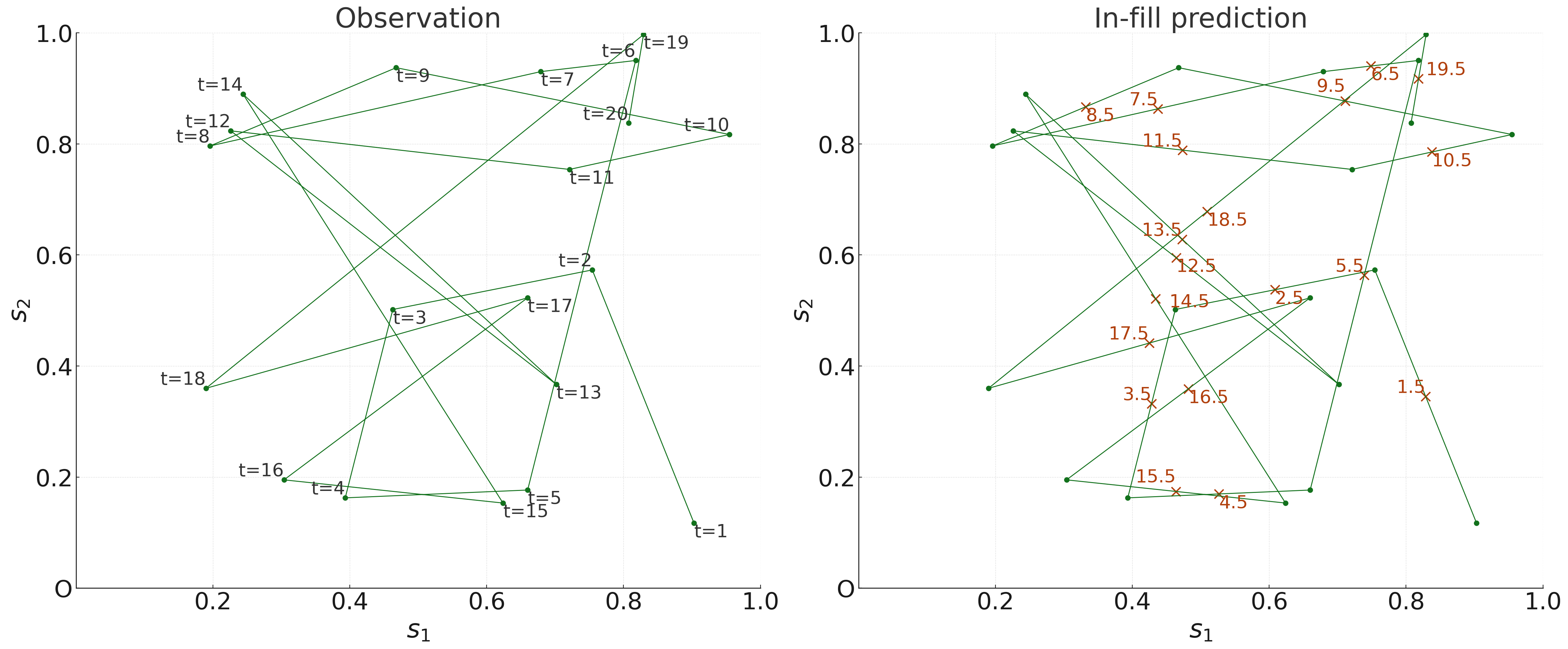
Figure 1. Left: observation points and trajectory (green line). Right: unobserved points (red cross marks) on the trajectory, where forecasts are made.

6.1. In-fill prediction

We consider a single trajectory $\gamma:\mathcal{T}\to\mathbb{R}^{2}$, where $\gamma(t)$ signifies the correspondence between the continuous closed interval $\mathcal{T}$ and a curve in $\mathbb{R}^{2}$. Because data are observed at discrete points on this trajectory, the accuracy of in-fill prediction is expected to improve as the number of discrete observed points grows. We consider interpolation of the outcome over a space-time trajectory composed of line segments. As an example of in-fill prediction, the conceptual diagram in Figure 1 depicts $T=20$ observations in the interval $\mathcal{T}=[1,20]$. The left panel displays the locations at each time point with the line segments comprising the trajectory shown by a green line. The right panel illustrates the space-time coordinates where we seek to predict the outcome.

We generate the data along a trajectory, which comprises our fixed domain, in accordance with the model in (4)–(7). We generate $300$ points on the trajectory over $t\in\mathcal{T}=[1,300]$ using $\gamma(t)=\gamma(t-1)+\mathcal{WN}(0,1)$, where $\mathcal{WN}(0,1)$ denotes white noise with zero mean and unit variance. We randomly include $n$ space-time coordinates over the trajectory and generate $n$ values of $z(\gamma(t),t)$ from the Gaussian process with $0$ mean and covariance kernel as (5). The true parameters defining the spatial-temporal process $z(\gamma(t),t)$ in (5) are $\phi_{1}=1/2$ and $\phi_{2}=1/2$. We then generate $y(\gamma(t),t)$ from (4) using elements of $x(\gamma(t),t)$ generated from $N(0,4)$ and $\beta_{j}(t)$ using a zero-centered Gaussian process with covariance kernel in (7) specified by $\xi=1/2$. Additionally, we set $\sigma=1$, $\delta_{\beta}=1$, and $\delta_{z}=1$.

For our experiments, we randomly include $n=20,40,\ldots,200$ points for training the data. Based on these observations, we evaluate the performance of interpolation over trajectories by comparing the posterior predictive means of $y(\gamma(t),t)$ and $z(\gamma(t),t)$ over $100$ randomly selected points on the trajectory that were excluded from the training data. For predictive stacking, a set of candidate parameters is specified with $\phi_{i}\in\{1,1/5\}$ for $i=1,2$ in (6), $\xi\in\{1,1/5\}$ in (7), and $\{3,1/3\}$ for both $\delta_{\beta}$ and $\delta_{z}$ in (5) and (7). We employ $20$-fold cross-validation to obtain the stacking weights described in Sections 4.1 and 4.2 and use posterior estimates drawn from (13). All our subsequent posterior summaries refer to (13). Furthermore, we implement $M_{0}$, an oracle method with the true parameters assigned and Bayesian model averaging (BMA, Hoeting et al. (1999)) with a uniform prior on candidate models, which yields a weighted average of multivariate t-distributions; see the Appendix for details on BMA. As measures of performance, we adopted three metrics: mean squared prediction error (MSPE) and mean squared error for $z$ (MSE$z$) for stacking of means, and mean log predictive density (MLPD) for predictive stacking of distributions.

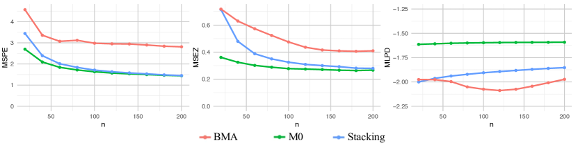
Figure 2. Predictive performances of stacking, BMA and $M_{0}$ (method with the oracle parameters) when $n$ grows from $20$ to $200$. Left: MSPE (mean squared prediction error). Middle: MSE$z$ (mean squared error for $z$). Right: MLPD (mean log predictive density). We clearly see stacking outperform BMA as it approaches the oracle much more rapidly with increasing $n$.

Figure 2 illustrates the overall predictive error behavior, where we generated 50 different datasets and report the average of the aforementioned metrics over the different datasets. The left and center panels, which plot MSPE and MSE$z$, respectively, demonstrate that an increasing number of points in the training data ($n$) over the fixed domain (trajectory) enhances the precision of predictions for outcomes and spatial effects. Similarly, the right panel reveals improvement in predictive accuracy in terms of MLPD as $n$ increases. Notably, stacking significantly outperforms BMA as its metrics approach those for the oracle model more rapidly with increasing $n$. While results established in Theorems 1–3 apply to Euclidean domains for theoretical tractability, our empirical findings on non-Euclidean trajectories in this experiment still appear to be consistent with those theoretical results.

6.2. Estimation performances of proposed models

We conducted simulation experiments to assess both discrete- and continuous-time trajectory models, comparing their performance in terms of estimation errors and model fitting. First, we sampled data along with the discrete time trajectory model in (2)–(3). We generated $n=T=50$ and $70$ points for two experiments on a trajectory using the same random walk model for $\gamma(t)$ as in Section 6.1. We take $p=2$ in (2) and generate initial values for the elements of ${\beta}_{0}$ and ${z}_{0}$ from $N({0},4)$. With these fixed initial values, we sequentially generate ${\beta}_{t}$ and ${z}_{t}$ using the autoregressive specification (see Section 2.2) with $\delta_{\beta}=1$, $\delta_{z}=1$, $\sigma=1$ and with $K_{\phi}$ taken as the Matérn kernel, introduced in Section 5.4, with $\phi=1/7$ and $\nu=1$. Each element of ${x}_{t}(\gamma(t))$ is generated from $N(0,4)$ and fixed thereafter. Then, $y_{t}(\gamma(t))$ is generated using (2).

We generated $30$ different datasets through the above procedure and analyzed each of them using the models in (3) and (8). For predictive stacking, we set candidate parameters in (3) as $\phi\in\{1,1/10\}$, $\nu\in\{3,1/3\}$ and $\{5,1/5\}$ for both $\delta_{\beta}$ and $\delta_{z}$. For (8), we consider $\phi_{i}\in\{3,1/10\}$ for $i=1,2$, $\xi\in\{3,1/10\}$, and $\{3,1/3\}$ for $\delta_{\beta}$ and $\delta_{z}$. We employed $20$-fold expanding window cross-validation and selected the stacking weights described in Sections 4.1 and 4.2. Additionally, we estimated a non-spatial dynamic linear model (NSDLM),

$$y_{t}={x}_{t}^{\top}{\beta}_{t}+\eta_{1t},\quad\eta_{1t}\overset{\mathrm{i.i.d.}}{\sim}N({0},\sigma^{2});\qquad{\beta}_{t}={\beta}_{t-1}+\eta_{2t},\quad\eta_{2t}\overset{\mathrm{i.i.d.}}{\sim}N({0},W).$$

We assign priors ${\beta}_{0}\sim N({0},10I_{2})$, $W\sim IW(10,10I_{2})$ and $\sigma\sim IG(1/2,1/2)$. This model solely captures the temporal structure of the data without accounting for spatial locations.

We use MSE to compare the posterior predictive means for $y_{T+1}$ with the underlying signals in (2). Similarly, we use relative mean squared errors (rMSE) defined as $\sum_{t=1}^{T}(\widehat{\omega}_{t}-\omega_{t})^{2}/(\sum_{t=1}^{T}\omega_{t}^{2})$, where $\widehat{\omega}_{t}$ denotes the posterior mean and $\omega_{t}$ is the true value, to compare our inferential effectiveness, We apply rMSE to each element of $\beta_{t}$ and $z_{t}$, while we use $(\widehat{\sigma}-\sigma)^{2}/\sigma^{2}$ for $\sigma$. To evaluate model fit, we report MLPD, the deviance information criterion (DIC, Spiegelhalter et al., 2002) and the widely applicable information criterion (WAIC, Watanabe, 2010).

	n=50			n=70
Metrics	Discrete	Continuous	NSDLM	Discrete	Continuous	NSDLM
MSE$y$	1.038	1.028	2.171	0.996	0.989	2.163
rMSE$z$	0.761	0.908	—	0.766	0.915	—
rMSE$\beta_{1}$	0.166	0.576	1.709	0.197	0.620	2.042
rMSE$\beta_{2}$	0.201	0.648	1.698	0.142	0.570	1.651
rMSE$\sigma$	0.564	0.583	0.295	0.208	0.227	0.298
MLPD	-1.793	-1.772	-1.774	-1.784	-1.743	-1.784
DIC	50.682	151.500	417.482	62.454	216.382	586.966
WAIC	43.674	225.633	1909.787	80.012	269.553	2058.120

Table 1. Comparison of methods for data generated by discrete-time trajectory models. MSE$y$ denotes the mean squared error of the response variable $y$, rMSE$z$ is the relative MSE (rMSE) of the spatial-temporal effect $z$, rMSE$\beta_{1}$ and rMSE$\beta_{2}$ are the rMSE of the two slope coefficients, respectively, and rMSE$\sigma$ is the rMSE of the $\sigma$.

Table 1 presents comparisons among the three models with regard to predictive evaluation for the datasets generated by the discrete-time model. The entries represent the average values of the metrics over $30$ datasets. The discrete and continuous trajectory models clearly outperform NSDLM, as the latter is unable to capture spatial structure. We note insignificant differences between the discrete and continuous time models with respect to MSE of $y$ (MSE$y$) and the rMSE of $z$ (rMSE$z$). This indicates that both methods are nearly comparable in their ability to evaluate the true signal and spatial-temporal effects in this dataset and indicates the competitiveness of the continuous model. However, the discrete model outperforms the continuous model in terms of rMSE of the regression coefficients in $\beta$ (rMSE$\beta_{1}$ and rMSE$\beta_{2}$), where the discrete model unsurprisingly captures its own data generating process better than the continuous model. For model evaluation, the discrete-time model excels in terms of DIC and WAIC, although the MLPDs are nearly equal across all the models.

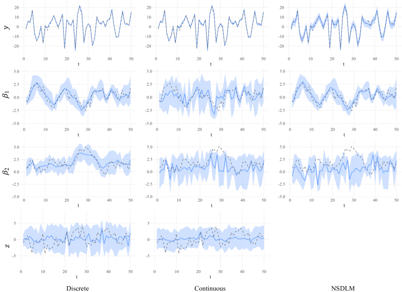
Figure 3. Posterior bands of parameters obtained by discrete time, continuous time and NSDLM models for one representative dataset generated from a discrete time trajectory model with $n=50$. Each panel represents the posterior summaries for $y$, $z$ and $\beta$, with solid blue lines representing posterior means, and the shaded blue bands representing the 95% credible intervals, and dashed lines representing true values.

Figure 3 presents the posterior means (solid curve) for $y_{t}(\gamma(t))$, $z_{t}(\gamma(t))$ and the two regression coefficients comprising each $\beta_{t}$ as a function of time for one representative dataset with $n=50$ in the simulation experiment. Also shown are the true values generating the data in the form of a dashed line. We see that the posterior bands from the discrete model are more effective in containing the dashed line (truth) with the continuous model and the NSDLM still performing fairly well, although both prominently miss the truth for the second coefficient in $\beta$.

Next, we generated $30$ datasets from the continuous-time trajectory model described in (4)–(7). We generate $n=T=50$ and $70$ points on the trajectory by the same random walk as in Section 6.1. The true parameters for spatial-temporal process $z(\gamma(t),t)$ in (5) are $\phi_{1}=1/2,\phi_{2}=1/2$ and $\delta_{z}=1$. Then, we produce $y$ from (4) using $\sigma=1$, each $\beta_{j}$ generated from (7) with $\xi=1/2$ and $\delta_{\beta}=1$ and the elements of $x(\gamma(t),t)$ generated from $N(0,4)$.

We analyzed each of the $30$ datasets using the continuous time and discrete time trajectory models. For predictive stacking, a set of candidate parameters of the discrete model in (3) was set to $\phi\in\{2,1/2\}$, $\nu\in\{2,1/2\}$, $\delta_{\beta}\in\{1/2,1/10\}$ and $\delta_{z}\in\{1/2,1/10\}$. For the continuous model in (8), we set $\phi_{i}\in\{1,1/4\}$ for $i=1,2$, $\xi\in\{1,1/4\}$, and $\delta_{\beta}$ and $\delta_{z}$ in $\{3,1/3\}$. We employed $20$-fold expanding window cross-validation to determine the stacking weights as in the earlier example.

	n=50			n=70
Metrics	Discrete	Continuous	NSDLM	Discrete	Continuous	NSDLM
MSE$y$	0.810	0.725	0.997	0.863	0.674	0.902
rMSE$z$	0.508	0.311	—	0.434	0.264	—
rMSE$\beta_{1}$	0.088	0.093	2.737	0.109	0.134	6.282
rMSE$\beta_{2}$	0.078	0.150	3.041	0.103	0.075	1.914
rMSE$\sigma$	0.346	0.498	0.043	0.480	0.506	0.042
MLPD	-1.279	-1.272	-1.414	-1.350	-1.213	-1.394
DIC	139.965	124.344	222.319	177.520	173.052	284.848
WAIC	132.214	148.231	304.411	167.744	213.590	385.777

Table 2. Comparison of methods for data generated by continuous-time trajectory models. MSE$y$ represents the mean squared error of the denoised response variable $y$, rMSE$z$ the relative MSE (rMSE) of the spatial-temporal effect $z$, rMSE$\beta_{1}$ and rMSE$\beta_{2}$ the rMSE of the coefficient $\beta_{1}$ and $\beta_{2}$, respectively, and rMSE$\sigma$ the rMSE of the $\sigma$.

The results of the predictions by the three methods are presented in Table 2. As in Table 1, the continuous and discrete time models outperform NSDLM. The accuracy of the response variable $y$ and spatial-temporal effect $z$ indicate that the continuous model performs better than the discrete model. Regarding the model fitting, again as seen in Table 1, we see that both the continuous and discrete time models excel over NSDLM.

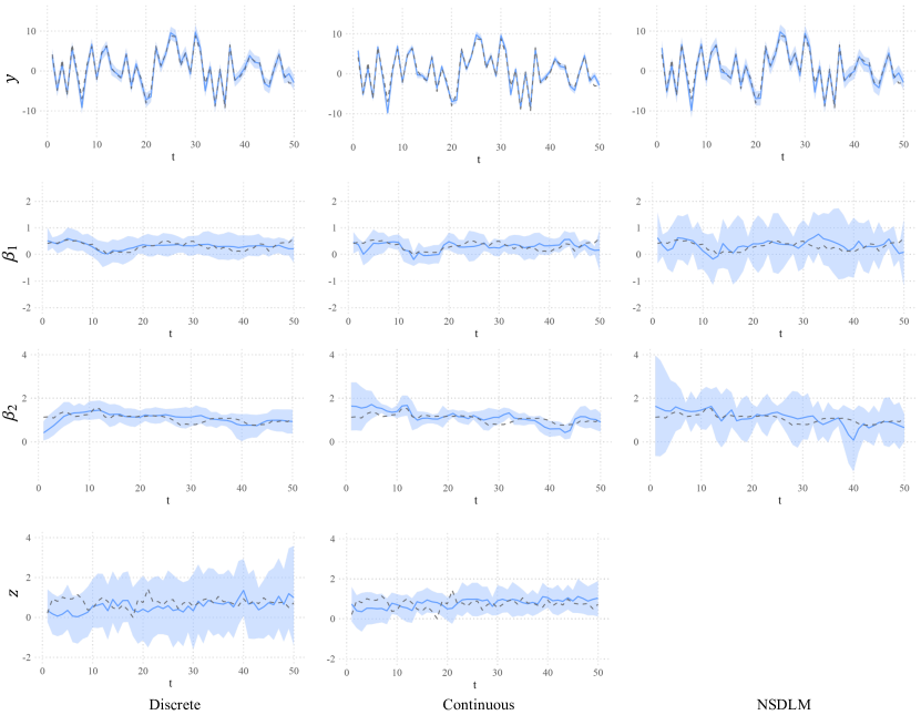
Figure 4. Posterior distributions of parameters obtained by discrete time, continuous time and NSDLM models for one representative dataset generated from a continuous time trajectory model. The top panels display histograms of the posterior distribution of $\sigma$. The others show posterior summaries for $y$, $z$ and $\beta$, with solid blue lines representing posterior means, shaded blue areas representing 95% credible intervals, and dashed lines representing true values.

Figure 4 is the analogue of Figure 3 for a representative dataset from the continuous time experiment showing posterior mean and 95% posterior interval for $y(\gamma(t),t)$, $z(\gamma(t),t)$ and two slopes as a function of time. While all three methods seem comparable in their ability to capture the truth (dashed line), the precision for the continuous model is higher than the other two models with NSDLM clearly having the widest bands for the regression slopes.

Method	Data Generating Process
	Discrete	Continuous
Discrete	$0.80$ (${0.54},{1.22}$)	$0.10$ ($0.06,0.16$)
Continuous	$8.77$ ($2.04,18.51$)	$1.02$ (${0.74},{1.48}$)

Table 3. Posterior summary of $\sigma^{2}$ of each method on each scenario when $n=50$. The true value of $\sigma^{2}$ is $1$. Both $\delta_{z}$ and $\delta_{\beta}$ are fixed to the true values.

Finally, we turn to the stacked posterior inference for $\sigma^{2}$ in Table 3. We present the posterior mean and the $95\%$ credible intervals obtained from one representative dataset generated by the discrete-time model and another from the continuous-time model when both $\delta_{\beta}$ and $\delta_{z}$ are fixed at their true values and $n=50$. The $2\times 2$ table presents the stacked estimates for $\sigma^{2}$ when each of these models is estimated from the two representative datasets. We find that the credible intervals from the discrete and continuous time models are able to capture the true value ($\sigma=1$) for the data generated from them, which seems to be consistent with the result in Theorem 1, but may not be able to capture the true value of $\sigma$ when they are not the data generating model. Furthermore, if $\delta_{\beta}$ and $\delta_{z}$ are not specified at their true values, inference for $\sigma^{2}$ suffers. This phenomenon has also been investigated by Zhang et al. (2023) and is largely attributable to the fact that $\sigma^{2}$ is not consistently estimable in Gaussian process models (Zhang, 2004; Tang et al., 2021).

7. Application

We apply the continuous space-time model (4) to the actigraph dataset, sourced from the Physical Activity through Sustainable Transport Approaches in Los Angeles (PASTA-LA), and described in detail in Alaimo Di Loro et al. (2023). Actigraph data are collected through wearable devices including sensors and a smartphone application, providing high-resolution and repeatable measurements for monitoring human activity. There is a growing body of research on the statistical relationships with physical activity measures, such as energy expenditure measures (EE) (Crouter et al., 2006; Freedson et al., 2012; Taraldsen et al., 2012) and the Metabolic Equivalent of Task (MET) (Ishikawa-Takata et al., 2008; Lyden et al., 2014; Staudenmayer et al., 2015; Bai et al., 2018). Here, we consider the instantaneous body vector Magnitude of Acceleration (MAG) as the primary endpoint of our analysis (Doherty et al., 2017). Further discussion about the conversion of MAG into energy expenditure measures is reported in (Alaimo Di Loro et al., 2023).

A major aim of this study is to estimate an individual’s MAG along a traversed path after accounting for the impact of explanatory variables (e.g., environmental features, risk factors) on metabolism. These estimates from the continuous time model, which represent statistical learning of an individual’s physical activity profile on any given day, are then used to predict the subject’s metabolic activity on any arbitrary trajectory and comprise a personalized recommendation system for the subject. The models we have developed here can yield more effective pathways and environments to enhance physical activity levels of subjects and lead to overall improvements in metabolic levels.

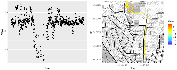
Figure 5. $650$ time-series points of log-transformed MAG (left), and spatial movement of the person with log-transformed MAG values (right).

Focusing on one individual, which is often the goal in personalized health science research seeking data driven recommendation systems for metabolic activity, we consider recordings on the MAG observed at $650$ unevenly spaced time points. The left panel of Figure 5 displays the values of the recorded MAG and the right panel plots the MAGs over the path traversed by this individual. We fit the continuous time model in (4) using “Slope”, representing the gradient at the spatial location, and “NDVI”, representing normalized vegetation index, which is a measure of greenness at the location, as the two explanatory variables in $x(\gamma(t),t)$, where $\gamma(t)$ is recorded as the subject’s coordinates along the trajectory using information from GPS. For predictive stacking, the candidates for the parameters $\phi_{1},\phi_{2},\xi$ were set $\{100,1\}$ and those for $\delta_{\beta},\delta_{z}$ were set $\{20,1/5\}$. Of the $650$ observations, $130$ data were randomly selected and used as test data, and the remaining $520$ data were utilized as training data. We computed the posterior distributions for both the continuous time trajectory model and Bayesian linear regression on the training data and performed predictions. For comparison, we applied a Bayesian linear regression model to this data using the “brm” function from the (“brms” package Bürkner, 2023) in R and adopted default priors, that is, $t_{3}(0,2.5)$ prior for $\sigma$ and flat priors for coefficients of the explanatory variables.

	Bayesian linear regression	Continuous time trajectory model
MSPE	0.787	0108
MLPD	-1.312	-0.883

Table 4. MSPE and MLPD of the interpolations by Bayesian linear regression and the continuous time trajectory model with predictive stacking.

Table 4 indicates the superiority of the proposed methods over Bayesian linear regression. Notably, there is a significant difference in MSPE with the proposed model exhibiting considerably lower errors compared with Bayesian linear regression. The MLPD, indicating the goodness of the posterior distribution, also demonstrates that the proposed model outperforms Bayesian linear regression. This superior performance is likely attributable to accounting for the spatial-temporal structure in the data. The incorporation of spatial and temporal structure into a model allows for a more detailed depiction of the data, resulting in more precise predictions. By contrast, Bayesian linear regression does not account for the information, confirming its limitations for real data where the spatial-temporal information is significant.

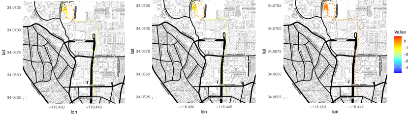
Figure 6. Left: 130 observed test data of $y$. Middle: 130 predictions of $y$ by the continuous time trajectory model. Right: 130 predictions of $z$ by the continuous time trajectory model.

Figure 6 presents 3 maps to display spatial interpolation for actigraph data. The left panel plots the 130 raw observations over a path traversed by the subject under consideration. The values of the (transformed) MAG are calibrated using colors shaded from deep blue (lowest) to red (highest). The middle panel displays the interpolated MAGs using the posterior predictive means from the stacked posterior distribution in (13) derived from the continuous time model. We note that estimated MAGs along this path effectively capture the features of the observed MAGs. The right panel depicts the posterior predictive means of the latent process using (13) derived from the continuous time model. The variation in the right panel suggests that substantial spatial structure remains on the trajectory after accounting for “Slope” and “NDVI”. The utility of the middle and right panels are distinct. The former is useful for understanding MAG as a feature associated with a path or trajectory. Our framework is able to predict the MAG at a completely arbitrary path, where no measurements have been measured, for a subject had an individual with a given set of personalized health attributes traversed that path. The latter, on the other hand, helps investigators glean lurking factors that may explain some of the residual spatial structure on a trajectory after accounting for the explanatory variables such as “Slope” or “NDVI”.

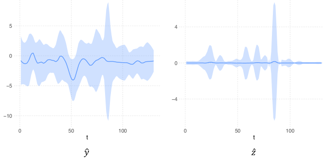
Figure 7. Left: Posterior predictive bands of $y$ obtained by continuous time trajectory model. Right: Posterior predictive bands of $z$ obtained by continuous time trajectory model.

Another key inferential element for spatial energetics is the estimate of an individual’s daily profile of MAG, which allows medical professionals to recommend changes, if and as deemed appropriate, in the subject’s daily mobility habits. As in the preceding figure, here, too, these daily profiles can be plotted for the outcome or for the residual. Figure 7 presents these plots. The left panel plots the posterior predictive mean and 95% credible interval band for the MAG along the hours of the day to elicit the daily physical activity pattern of the subject and to better distinguish times of higher activity from those with lesser activity. The right panel presents the analogous plot for the residual process after accounting for trajectory effects represented by slope and greenness.

Given the complications associated with streaming measurements at high resolutions from wirelessly operating wearable devices, it is customary to encounter swaths of time intervals that have not recorded measurements either due to technical malfunction or user behavior. Our model based inferential framework uses the posterior predictive distributions to impute such missing values. The left panel in Figure 8 presents the reconstructed MAG for the subject under consideration at some epochs using the continuous time model. The right panel presents posterior predictive credible intervals that reveal the model’s ability to effectively capture 130 held-out values for predictive validation.

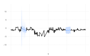
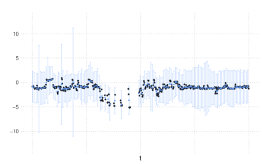
Figure 8. Left: Bayesian imputation of missing measurements at some epochs using the continuous time trajectory model. Right: 95% credible intervals and posterior predictive means of 130 held-out MAG values using the continuous time trajectory model.

Finally, we compare the continuous time, discrete time and NSDLM using DIC and WAIC. For this, we extract $150$ distinct time points from the above data, ensuring that they are equally spaced and compatible with the discrete-time trajectory model in (2) and the NSDLM introduced in Section 6.2. For stacking of (2), the candidates for the parameters were $\phi\in\{1,1/10\}$, $\nu\in\{1,1/3\}$ and $\delta_{\beta},\delta_{z}\in\{5,1/5\}$. Table 5 reveals that the continuous time trajectory model is preferred (lower values) to the others in either of these metrics, while the discrete time model considerably outperforms NSDLM. In designing a physical activity recommending system that trains one model, our analysis suggests using the continuous time model is preferable although the discrete time model should also be competitive.

	Continuous	Discrete	NSDLM
DIC	-60.318	-17.996	93.249
WAIC	-87.106	-40.116	150.508

Table 5. Goodness of fit of the continuous time trajectory model, the discrete time trajectory model, and the NSDLM, measured by DIC and WAIC.

8. Summary

We have devised a Bayesian inferential framework for spatial energetics that aims to analyze data collected from wearable devices containing spatial information over paths or trajectories traversed by an individual. Data analytic goals include estimating underlying spatial-temporal processes over trajectories that are posited to be generating the observations. A salient requirement for appropriately modeling spatial dependence in such applications is to model spatial locations as a function over time. We introduce such dependence in two broad classes of models: one that treats time as discrete and another that treats time as continuous. The former builds on Bayesian dynamic linear models and the latter employs spatial-temporal covariance functions to specify the underlying process. For conducting inference, we propose Bayesian predictive stacking as an effective method, where fully tractable conjugate posterior distributions up to certain parameters are assimilated, or stacked, to deliver Bayesian inference using a stacked posterior. Our framework offers some theoretical results to justify why predictive stacking renders effective posterior inference.

Computer Programs

Computer programs used in the manuscript for generating data for our simulation experiments in Section 6 and the application presented in Section 7 have been developed for execution in the R statistical computing environment. The programs are available for download in the publicly accessible GitHub repository https://github.com/TomWaka/BayesianStackingSpatiotemporalModeling.

Appendix

Notation

The notation $[A\mid B]$ represents a block matrix formed by horizontally concatenating $A\in\mathbb{R}^{p\times q}$ and $B\in\mathbb{R}^{p\times r}$. Given a $p\times q$ matrix $A$ and a $m\times n$ matrix $B$, $A\otimes B$ is the Kronecker product producing a $pm\times qn$ block matrix with $(i,j)$th block is $a_{ij}B$, while $A\oplus B$ denotes the block diagonal matrix with $A$ and $B$ along the diagonal. A $p$-dimensional random variable $x$ is said to be distributed as a multivariate t-distribution $t_{\nu}(\mu,\Sigma)$ with parameters $(\nu,\mu,\Sigma)$ if it has the density

$$f(x;\mu,\Sigma,\nu)=\frac{\Gamma(\frac{\nu+p}{2})}{\Gamma(\frac{\nu}{2})(\nu\pi)^{p/2}\mathrm{det}(\Sigma)^{1/2}}\left(1+\frac{1}{\nu}(x-\mu)^{\top}\Sigma^{-1}(x-\mu)\right)^{-\frac{\nu+p}{2}},$$

where $\Gamma(\cdot)$ is the gamma function and $\mathrm{det}(\cdot)$ is the determinant of a matrix.

Proof of Lemma 1

Proof.

Let $\mathbb{P}_{t}^{*}$ be the probability law endowed on a finite spatial realization of $y_{t}(s)$ with true parameters and let $\mathbb{P}_{t}^{\prime}$ be that with parameters $(\sigma_{*},\phi^{\prime},\delta_{z}^{\prime})$. For all $t=1,\ldots,T$, the Matérn based model without trend (i.e., $\beta=0$) is

$$y_{t}(s) =z_{t}(s)+\eta_{1},\quad\eta_{1}\overset{\mathrm{i.i.d.}}{\sim}N(0,\sigma^{2}),$$

$$z_{t}(s) \overset{\mathrm{ind}}{\sim}GP\left(0,\sigma^{2}\Delta_{zt}^{2}K_{\phi}(\cdot,\cdot)\right),$$

where $\Delta_{zt}^{2}=\sum_{j=1}^{t}\delta_{z}^{2j}(\alpha\sigma)^{2(j-1)}$. Applying Theorem 2.1 in Tang et al. (2021), we obtain that $\mathbb{P}_{t}^{\prime}$ and $\mathbb{P}_{t}^{*}$ are equivalent. The equivalence of the joint distributions follows. ∎

Intuitive images of observational assumption

All theorems in Section 5.4 place the following restriction on the nature of $n$ spatial locations within a bounded region $\mathcal{S}$:

$$\max_{s\in\mathcal{S}}\min_{1\leq i\leq n}|s-s_{i}|\asymp n^{-\frac{1}{d}}.$$

Figure 9 presents a depiction of the above assumption, which indicates that the spatial locations are scattered evenly.

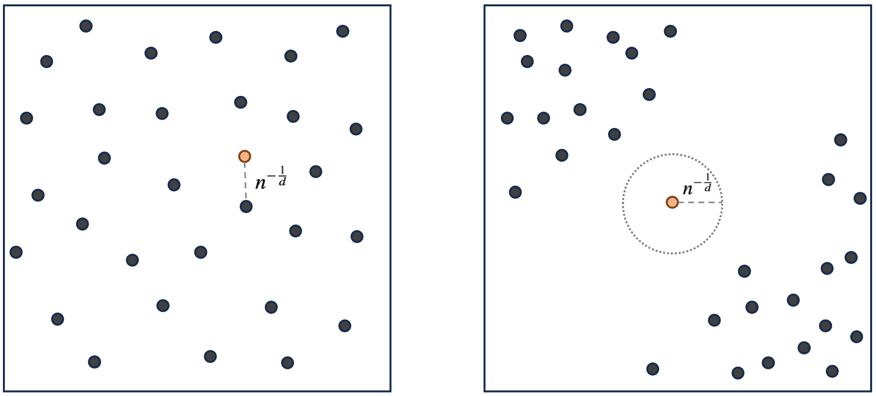
Figure 9. Left: scattered points such that $\max_{s\in\mathcal{S}}\min_{1\leq i\leq n}|s-s_{i}|\asymp n^{-\frac{1}{d}}$. Right: a polarized set of points on the domain such that $\max_{s\in\mathcal{S}}\min_{1\leq i\leq n}|s-s_{i}|>n^{-\frac{1}{d}}$.

Proof of Theorem 1

Before proceeding with the proof of Theorem 1, we recall the following lemma about the convergence of a random series.

Lemma 2.

Let $\{X_{i}:i\in\mathbb{N}\}$ be independent random variables with finite second moment and $\{a_{i}\in\mathbb{R}^{+}:i\in\mathbb{N}\}$ be an increasing positive number sequence such that $a_{i}\uparrow\infty$. If $\sum_{i=1}^{\infty}Var(X_{i})/a_{i}^{2}<\infty$, it holds that

$$\frac{\sum_{i=1}^{n}(X_{i}-\mathbb{E}[X_{i}])}{a_{n}}\to 0\quad\mathrm{a.s.}.$$

Proof.

Let $Y_{i}=(X_{i}-\mathbb{E}[X_{i}])/a_{i}$. Since $\mathbb{E}[Y_{i}]=0$ and $\sum_{i=1}^{\infty}Var(Y_{i})<\infty$, it follows from Kolmogorov’s one series theorem (e.g., Theorem 2.5.6. in Durrett (2019)) that $\sum_{i=1}^{\infty}Y_{i}<\infty$ almost surely. Then, from Kronecker’s lemma, $a_{n}^{-1}\sum_{i=1}^{n}(X_{i}-\mathbb{E}[X_{i}])$ converges to $0$ almost surely. ∎

We now present the main proof of Theorem 1.

Proof.

We rewrite the notation introduced in Proposition 1 as $n_{t}=n_{t-1}+n$, $n_{t}s_{t}=n_{t-1}s_{t-1}+({y_{t}}-{f}_{t})Q_{t}^{-1}({y_{t}}-{f}_{t}),{f}_{t}=\alpha{m}_{t-1},Q_{t}=R_{t}+I_{n},{m}_{t}={f}_{t}+R_{t}Q_{t}^{-1}({y}_{t}-{f}_{t}),R_{t}=\alpha^{2}W_{t-1}+\delta_{z}^{{}^{\prime}2}K_{\phi^{\prime}}(\chi)$ and $W_{t}=R_{t}-R_{t}^{\mathrm{\scriptscriptstyle T}}Q_{t}^{-1}R_{t}$. Here, we prove $\frac{n_{t}s_{t}-n_{t-1}s_{t-1}}{n}\rightarrow t\sigma_{*}^{2}$ by mathematical induction on $t$.

The base step $t=1$ yields

$$n_{1}s_{1}-n_{0}s_{0} =({y}_{1}-\alpha{m}_{0})^{\mathrm{\scriptscriptstyle T}}Q_{1}^{-1}({y}_{1}-\alpha{m}_{0})$$

$$={y}_{1}^{\mathrm{\scriptscriptstyle T}}\left((\alpha^{2}+\delta_{z}^{\prime 2})K_{\phi^{\prime}}(\chi)+I_{n}\right)^{-1}{y}_{1}$$

Let $U_{n}$ be a unitary matrix such that $U_{n}K_{\phi^{\prime}}U_{n}^{\mathrm{\scriptscriptstyle T}}$ is diagonal and let $\lambda_{i}^{(n)}$ be the $i$th eigenvalue of $K_{\phi^{\prime}}$ for $i=1\ldots,n$. Since $U_{n}{y}_{1}$ follows a zero-centered multivariate normal distribution with a diagonal covariance matrix whose $i$th diagonal is $\sigma_{*}^{2}(1+\delta_{z}^{\prime 2}\lambda_{i}^{(n)})$ under $\mathbb{P}^{\prime}$, we obtain

$$n_{1}s_{1}-n_{0}s_{0}=\sum_{i=1}^{n}\frac{\sigma_{*}^{2}(1+\delta_{z}^{\prime 2}\lambda_{i}^{(n)})}{1+(\alpha^{2}+\delta_{z}^{\prime 2})\lambda_{i}^{(n)}}u_{i}^{2},$$

where $u_{i}$ follows the standard normal distribution. Let $A_{i}=\left(\sigma_{*}^{2}(1+\delta_{z}^{\prime 2}\lambda_{i}^{(n)})\right)\big{/}\left(1+(\alpha^{2}+\delta_{z}^{\prime 2})\lambda_{i}^{(n)}\right)$. Because $\lambda_{i}^{(n)}\leq Cni^{-2\nu/d-1}$ for all $i=1,\ldots,n$ from Corollary 2 in Tang et al. (2021), $(\sum_{i=1}^{n}A_{i})/(n\sigma_{*}^{2})$ converges to $1$ as $n\to\infty$. By $\sum_{i=1}^{\infty}A_{i}^{2}/i^{2}<\infty$ and Lemma 2, we obtain

$$\frac{n_{1}s_{1}-n_{0}s_{0}}{n}=\frac{1}{n}\sum_{i=1}^{n}A_{i}u_{i}^{2}~{}\rightarrow~{}\sigma^{2}_{*},\quad\mathbb{P}^{\prime}-\text{a.s.}$$

Owing to the equivalence of $\mathbb{P}_{*}$ and $\mathbb{P}^{\prime}$, $\frac{n_{1}s_{1}-n_{0}s_{0}}{n}\rightarrow\sigma^{2}_{*}$ holds $\mathbb{P}_{*}$-almost surely.

Then, as an inductive step, we assume that $\frac{n_{t}s_{t}}{n}\rightarrow t\sigma_{*}^{2}$ holds $\mathbb{P}_{*}$-almost surely and we consider the next period. We have

$$n_{t+1}s_{t+1}-n_{t}s_{t}=({y}_{t+1}-\alpha{m}_{t})^{\mathrm{\scriptscriptstyle T}}Q_{t+1}^{-1}({y}_{t+1}-\alpha{m}_{t}),$$

where $Q_{t+1}=(I_{n}+\alpha^{2}W_{t}+\delta_{z}^{\prime 2}K_{\phi^{\prime}})$ and $W_{t}=R_{t}-R_{t}^{\mathrm{\scriptscriptstyle T}}Q_{t}^{-1}R_{t}$. Let $\lambda_{t,i}^{(n)}$ be the $i$th eigenvalue of $W_{t}$. Because $W_{t}=(R_{t}^{-1}+I_{n})^{-1}$ and $R_{t}=\alpha^{2}W_{t-1}+\delta_{z}^{\prime 2}K_{\phi^{\prime}}$, it holds that, under $\mathbb{P}^{\prime}$,

$$\lambda_{t,i}^{(n)}=\frac{(\alpha^{2}+\delta_{z}^{\prime 2})\lambda_{t,i}^{(n)}}{1+(\alpha^{2}+\delta_{z}^{\prime 2})\lambda_{t,i}^{(n)}}.$$

Note that $\lambda_{t,i}^{(n)}\to\left(\alpha^{2}+\delta_{z}^{\prime 2}\right)^{t}\lambda_{i}^{(n)}$ as $i\to\infty$. Then,

$$\frac{1}{n}({y}_{t+1}-\alpha{m}_{t})^{\mathrm{\scriptscriptstyle T}}Q_{t+1}^{-1}({y}_{t+1}-\alpha{m}_{t}) =\frac{1}{n}{y}_{t+1}^{\mathrm{\scriptscriptstyle T}}U_{n}^{\mathrm{\scriptscriptstyle T}}U_{n}Q_{t+1}^{-1}U_{n}^{\mathrm{\scriptscriptstyle T}}U_{n}{y}_{t+1}-\frac{2\alpha}{n}{y}_{t+1}^{\mathrm{\scriptscriptstyle T}}Q_{t+1}^{-1}{m}_{t}+\frac{\alpha^{2}}{n}{m}_{t}^{\mathrm{\scriptscriptstyle T}}Q_{t+1}^{-1}{m}_{t}$$

$$=\frac{1}{n}{y}_{t+1}^{\mathrm{\scriptscriptstyle T}}U_{n}^{\mathrm{\scriptscriptstyle T}}U_{n}Q_{t+1}^{-1}U_{n}^{\mathrm{\scriptscriptstyle T}}U_{n}{y}_{t+1}+o(1)$$

$$=\frac{1}{n}\sum_{i=1}^{n}\frac{\sigma_{*}^{2}+v^{\prime 2}\lambda_{i}^{(n)}}{1+\alpha^{2}\lambda_{t,i}^{(n)}+\delta_{z}^{\prime 2}\lambda_{i}^{(n)}}u_{i}^{2}+o(1)$$

where $u_{i}\sim N(0,1)$. The second equality holds because when we recursively expand $m_{t}$ by its definition, we find that $m_{t}$ includes a factor of $R_{t}$. Then, the second and third terms are $o(1)$ due to the eigenvalue decay of $R_{t}$. Hence, using Lemma 2 and the equivalence of the distributions, we obtain

$$\frac{1}{n}\sum_{i=1}^{n}\frac{\sigma_{*}^{2}+v^{\prime 2}\lambda_{i}^{(n)}}{1+\alpha^{2}\lambda_{t+1,i}^{(n)}+\delta_{z}^{\prime 2}\lambda_{i}^{(n)}}u_{i}^{2}~{}\rightarrow~{}\sigma^{2}_{*},\quad\mathbb{P}_{*}-\text{a.s.}$$

Therefore, we have

$$\frac{n_{t+1}s_{t+1}}{n}\rightarrow(t+1)\sigma_{*}^{2},\quad\mathbb{P}_{*}-\text{a.s.}$$

This concludes the induction step and we conclude $\frac{n_{t}s_{t}-n_{t-1}s_{t-1}}{n}\rightarrow t\sigma_{*}^{2}$ holds for each $t=1,2,\ldots,T$. From Chebyshev’s inequality, $p(\sigma^{2}\mid\mathcal{D}_{\chi_{n},t})\rightsquigarrow\delta(\sigma_{*}^{2})$ holds $\mathbb{P}_{*}$-almost surely.

∎

Proof of Theorem 2

Proof.

Recall that $n_{t}=n_{t-1}+n$, $n_{t}s_{t}=n_{t-1}s_{t-1}+({y_{t}}-{f}_{t})Q_{t}^{-1}({y_{t}}-{f}_{t}),{f}_{t}=\alpha{m}_{t-1},Q_{t}=R_{t}+I_{n},{m}_{t}={f}_{t}+R_{t}Q_{t}^{-1}({y}_{t}-{f}_{t}),R_{t}=\alpha^{2}W_{t-1}+\delta_{z}^{{}^{\prime}2}K_{\phi^{\prime}}(\chi)$ and $W_{t}=R_{t}-R_{t}^{\mathrm{\scriptscriptstyle T}}Q_{t}^{-1}R_{t}$. We decompose the prediction error for the latent term $\widetilde{z}_{t}(s_{0})$ as

$$\mathbb{E}_{*}[(Z_{tn}(s_{0})-\widetilde{z}_{t}(s_{0}))^{2}] =\mathbb{E}_{*}[(Z_{tn}(s_{0})-\mathbb{E}[\widetilde{z}_{t}(s_{0})\mid\mathcal{D}_{\chi_{n},t}]+\mathbb{E}[\widetilde{z}_{t}(s_{0})\mid\mathcal{D}_{\chi_{n},t}]-\widetilde{z}_{t}(s_{0}))^{2}]$$

$$=\mathbb{E}_{*}[(Z_{tn}(s_{0})-\mathbb{E}[\widetilde{z}_{t}(s_{0})\mid\mathcal{D}_{\chi_{n},t}])^{2}+(\widetilde{z}_{t}(s_{0})-\mathbb{E}[\widetilde{z}_{t}(s_{0})\mid\mathcal{D}_{\chi_{n},t}])^{2}]$$

$$=\underbrace{\mathbb{E}_{*}[Var(Z_{tn}(s_{0}))]}_{E_{n,t}^{A}}+\underbrace{\mathbb{E}_{*}[(\widetilde{z}_{t}(s_{0})-\mathbb{E}[\widetilde{z}_{t}(s_{0})\mid\mathcal{D}_{\chi_{n},t}])^{2}]}_{E_{n,t}^{B}}$$ (16)

Focusing on the first term, $E_{n,t}^{A}$ in (16), we note the following distributions,

$$Z_{tn}(s_{0})\mid\mathcal{D}_{\chi_{n},t},\sigma^{2},{m}_{t} \sim N({c}_{0}^{\mathrm{\scriptscriptstyle T}}C^{-1}{m}_{t},\sigma^{2}\delta_{z}^{\prime 2}-{c}_{0}^{\mathrm{\scriptscriptstyle T}}C^{-1}{c}_{0}),$$

$${m}_{t}\mid\sigma^{2},{f}_{t},R_{t} \sim N({f}_{t},\sigma^{2}R_{t}(R_{t}+I_{n})^{-2}R_{t}),$$

where $C=\sigma^{2}\delta_{z}^{\prime 2}K_{\phi}(\chi_{n})$ and ${c}_{0}=(\sigma^{2}\delta_{z}^{\prime 2}K_{\phi}(s,s_{0}))_{s\in\chi_{n}}$. According to the law of total variance (Blitzstein and Hwang, 2019),

$$Var(Z_{tn}(s_{0})) =\mathbb{E}[Var(Z_{tn}(s_{0}))\mid\mathcal{D}_{\chi_{n},t},\sigma^{2},m_{t}]+Var(\mathbb{E}[Z_{tn}(s_{0})\mid\mathcal{D}_{\chi_{n},t},\sigma^{2},m_{t}])$$

$$=\sigma^{2}(\delta_{z}^{\prime 2}-\delta_{z}^{\prime 2}\{K_{\phi}(s,s_{0})\}_{s\in\chi_{n}}^{\mathrm{\scriptscriptstyle T}}K_{\phi}^{-1}(\chi_{n})\{K_{\phi}(s,s_{0})\}_{s\in\chi_{n}}$$

$$\quad+\{K_{\phi}(s,s_{0})\}_{s\in\chi_{n}}^{\mathrm{\scriptscriptstyle T}}K_{\phi}^{-1}(\chi_{n})R_{t}(R_{t}+I_{n})^{-2}R_{t}K_{\phi}^{-1}(\chi_{n})\{K_{\phi}(s,s_{0})\}_{s\in\chi_{n}}^{\mathrm{\scriptscriptstyle T}}).$$

From Theorem 1 we know that $p(\sigma^{2}\mid\mathcal{D}_{\chi_{n},t})\to\delta(\sigma^{2}_{*})$ as $n\to\infty$ under $\mathbb{P}_{*}$. We also obtain

$$E_{n,t}^{A} =\sigma_{*}^{2}(\delta_{z}^{\prime 2}-\delta_{z}^{\prime 2}\{K_{\phi}(s,s_{0})\}_{s\in\chi_{n}}^{\mathrm{\scriptscriptstyle T}}K_{\phi}^{-1}(\chi_{n})\{K_{\phi}(s,s_{0})\}_{s\in\chi_{n}}$$

$$\quad+\{K_{\phi}(s,s_{0})\}_{s\in\chi_{n}}^{\mathrm{\scriptscriptstyle T}}K_{\phi}^{-1}(\chi_{n})R_{t}(R_{t}+I_{n})^{-2}R_{t}K_{\phi}^{-1}(\chi_{n})\{K_{\phi}(s,s_{0})\}_{s\in\chi_{n}}^{\mathrm{\scriptscriptstyle T}})+o(1).$$

Furthermore, the second term in (16) can be represented as

$$E_{n,t}^{B}=\mathbb{E}_{*}\left[\left(\widetilde{z}_{t}(s_{0})-\{K_{\phi}(s,s_{0})\}_{s\in\chi_{n}}^{\mathrm{\scriptscriptstyle T}}K_{\phi}^{-1}(\chi_{n}){m}_{t}\right)^{2}\right].$$

The prediction error of $\widetilde{y}_{t}(s_{0})$ can be decomposed as

$$\mathbb{E}_{*}\left[(Y_{tn}(s_{0})-\widetilde{y}_{t}(s_{0}))^{2}\right] =\mathbb{E}_{*}\left[(Y_{tn}(s_{0})-\mathbb{E}[\widetilde{y}_{t}(s_{0})\mid\mathcal{D}_{\chi_{n},t}]+\mathbb{E}[\widetilde{y}_{t}(s_{0})\mid\mathcal{D}_{\chi_{n},t}]-\widetilde{y}_{t}(s_{0}))^{2}\right]$$

$$=\mathbb{E}_{*}\left[(Y_{tn}(s_{0})-\mathbb{E}[\widetilde{y}_{t}(s_{0})\mid\mathcal{D}_{\chi_{n},t}])^{2}+(\widetilde{y}_{t}(s_{0})-\mathbb{E}[\widetilde{y}_{t}(s_{0})\mid\mathcal{D}_{\chi_{n},t}])^{2}\right]$$

$$=\mathbb{E}_{*}\left[Var(Y_{tn}(s_{0}))\right]+\mathbb{E}_{*}\left[\left(Y_{t}(s_{0})-\mathbb{E}[\widetilde{y}_{t}(s_{0})\mid\mathcal{D}_{\chi_{n},t}]\right)^{2}\right]$$

$$\overset{n\to\infty}{\longrightarrow}2\sigma_{*}^{2}+E_{n,t}^{A}+E_{n,t}^{B}$$

∎

Proof of Theorem 3

Proof.

$$\mathbb{E}_{*}\left[\left(\widetilde{y}_{t}(s_{0})-\sum_{g=1}^{G}a_{g}\mathbb{E}_{g}[\widetilde{y}_{t}(s_{0})\mid\mathcal{D}_{\chi_{n},t}]\right)^{2}\right] =\sigma_{*}^{2}+\mathbb{E}_{*}\left[\left(\widetilde{z}_{t}(s_{0})-\sum_{g=1}^{G}a_{g}\mathbb{E}_{g}[\widetilde{z}_{t}(s_{0})\mid\mathcal{D}_{\chi_{n},t}]\right)^{2}\right]$$

$$=\sigma_{*}^{2}+\mathbb{E}_{*}\left[\left\{\sum_{g=1}^{G}a_{g}\left(\widetilde{z}_{t}(s_{0})-\mathbb{E}_{g}[\widetilde{z}_{t}(s_{0})\mid\mathcal{D}_{\chi_{n},t}]\right)\right\}^{2}\right].$$

By the Cauchy–Schwarz inequality, the second term is bounded by $G\left(\sum_{g}a_{g}^{2}\right)E_{n,t}^{B}$, which converges to zero. ∎

In-fill prediction of the discrete DLM model

Here, we examine the in-fill predictive performance for the discrete time Bayesian DLM. First, we introduce the data-generating process along with the model in (1). In the period $T=20$, we uniformly sample $n=50,100,\ldots,500$ spatial locations from the unit square $[0,1]^{2}\subset\mathbb{R}^{2}$ to generate training data (the left panel in Figure 10). The elements of initial values of the $2$-dimensional state vectors ${\beta}_{0}$ and ${z}_{0}$ are randomly generated from $N({0},4)$. With these initial values, we sequentially produce ${\beta}_{t}$ and ${z}_{t}$ using the autoregressive specification (see Section 2.1) with $\delta_{\beta}=1$, $\delta_{z}=1$, $\sigma=1$ and $K_{\phi}$ taken as the Matérn kernel and $\phi=1/7$ and $\nu=1$. Here, matrices $G_{\beta,t}$ and $G_{z,t}$ are configured as identity matrices of sizes $p$ and $n$, respectively, and are considered time-invariant. Then, we sampled each element of $X_{t}$ from $N(0,4)$ and $y$ from (1). In this setting, we consider the prediction of the one-step future data at all locations, including $n$ observed and $100$ newly sampled points, as shown in the right panel of Figure 10; the variation in the accuracy of spatial-temporal predictions with increasing spatial samples is of interest.

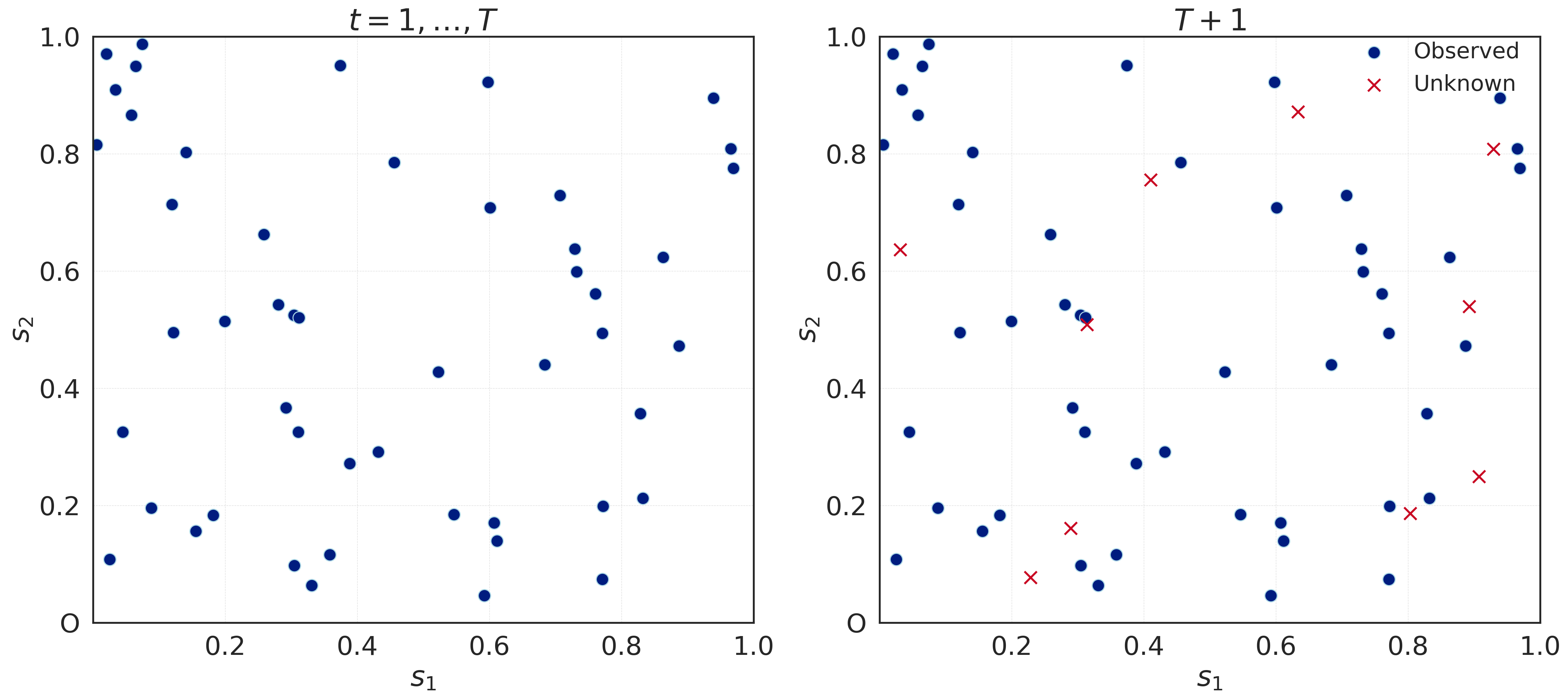
Figure 10. Space-time prediction (discrete case). Left: observation locations at $t=1,..,T$. Right: prediction locations at $T+1$, including observation points and new points.

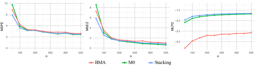
Figure 11. Prediction performances of stacking (our proposed method), Bayesian model averaging (BMA), and $M_{0}$ (method with the oracle parameters) when $n$ grows from $50$ to $500$. Left: mean squared prediction error (MSPE). Middle: mean squared error for $z$ (MSE$z$). Right: mean log predictive density (MLPD).

We generated $50$ different datasets using the above procedure and analyzed each dataset using the model in (1). For predictive stacking, we defined a set of candidate parameters: $\phi\in\{1/5,1/10\}$, $\nu\in\{2,1/2\}$, $\delta_{\beta}\in\{2,1/2\}$ and $\delta_{z}\in\{2,1/2\}$. We employed $20$-fold expanding window cross-validation and selected the stacking weights from $\Delta=\{\{a_{g}\}_{g=1}^{G}\mid\sum_{g=1}^{G}a_{g}=1,a_{g}\geq 0\}$ to yield a simplex of the candidate predictions (13). Furthermore, we implemented BMA with a uniform prior on candidate models and $M_{0}$, an oracle method with the true parameters assigned. As measures of performance, we adopted three metrics: mean squared prediction error (MSPE) and mean squared error for $z$ (MSE$z$) for stacking of means, and mean log predictive density (MLPD) for stacking of distributions.

Figure 11 provides an overview of these predictions, where we report the average of the aforementioned metrics over the $50$ datasets. The left and center panels illustrate the enhancement in predictions of both the outcome and spatial effects in the in-fill paradigm with more observed locations. The right panel demonstrates that distributional stacking consistently improves with an increasing $n$, as indicated by the log predictive density. These findings indicate that a higher number of spatial points (as long as the points are dispersed) improves predictions. Furthermore, the stacking results are generally better than those of BMA, underscoring the significance of weight determination.

Discussion of $E_{n,t}^{A}$  and $E_{n,t}^{B}$

Here, we elaborate on the asymptotic behaviors of $E_{n,t}^{A}$ and $E_{n,t}^{B}$, introduced in Section 5.4.

First, because $E_{n,t}^{A}$ does not have a closed form, we numerically investigate its decay as $n$ increases from $50$ to $1600$. The observation locations are uniformly sampled from the unit square $[0,1]^{2}\subset\mathbb{R}^{2}$. We compute $E_{n,t}^{A}$ with $\delta_{\beta}=\delta_{z}=\sigma=1$, $(\phi,\nu)\in\{(1/2,1),(1/5,1/2),(1/10,1/3)\}$ and $T\in\{2,20\}$. The upper panels in Figure 12 illustrate the predictive variance of $z$ in the absence of a trend, whereas the lower panel shows the predictive variance of $z$ when a trend is present. The training periods are $2$ and $20$ periods on the left and right sides, respectively. In all settings, the predicted variance decreases with an increasing sample size. The increase in $T$ indicates a faster decrease in predictive variance, suggesting that the rate is influenced by the training period $T$.

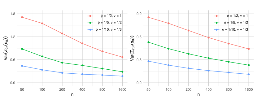
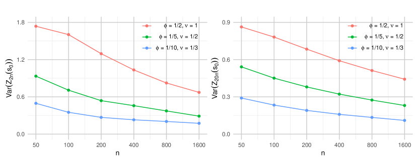
Figure 12. Decay of $E_{n,t}^{A}$ with an increasing sample size. The upper panels show predictive variances of $z$ without a trend, and the lower panels describe those with a trend. The left column shows those when the training period is $2$, while the right column illustrates those when the training period is $20$.

Next, we consider the decay of $E_{n,t}^{B}$. For simplicity, we assume $T=1$ and the space has dimensions of $1$. Here, we denote $\chi_{n}=\{i/n,i=-n,-n+1,\ldots,n-1,n\}\subset\mathbb{R}$, $\widetilde{\chi}_{n}=\{i/n,i\in\mathbb{N}\}\subset\mathbb{R}$. Let $\mathcal{D}_{-0,t}$ be data in $\chi_{n}\setminus\{0\}$ until time $t$, $\widetilde{\mathcal{D}}_{-0,t}$ be data in $\widetilde{\chi}_{n}\setminus\{0\}$ until time $t$, $e:=\mathbb{E}_{*}[\widetilde{z}(0)-\mathbb{E}[\widetilde{z}(0)\,|\,\mathcal{D}_{-0,t}]],$ and $\widetilde{e}:=\mathbb{E}_{*}[\widetilde{z}(0)-\mathbb{E}[\widetilde{z}(0)\,|\,\widetilde{\mathcal{D}}_{-0,t}]]$. The attenuation of $E_{n,t}^{B}$ with larger $n$ is then justified based on the following result from Zhang et al. (2023)

Theorem 4.

Assume $|e-\widetilde{e}|\to 0$ as $n\to\infty$. Then, the following holds as $n\to\infty$:

$$E_{n,t}^{B}\to 0.$$

Procedure of Bayesian Model Averaging

Bayesian Model Averaging for predictors is given by

$$p(\widetilde{y}\,|\,\mathcal{D})=\sum_{g=1}^{G}p_{g}(\widetilde{y}\,|\,\mathcal{D})p(M_{g}\,|\,\mathcal{D}),$$

where $\mathcal{D}$ is the dataset, $M_{g}$ is the $g$-th candidate model, $G$ is the number of candidate models, and $p(M_{g}\,|\,\mathcal{D})$ is the posterior probability of model $M_{g}$ given by

$$p(M_{g}\,|\,\mathcal{D})=\frac{p_{g}(\mathcal{D})p(M_{g})}{\sum_{l=1}^{G}p(\mathcal{D})p(M_{l})},$$

where $p(M_{g})$ is the prior probability of model $M_{g}$ and $p_{g}(\mathcal{D})$ is the marginal likelihood of model $M_{g}$. If the prior is assumed to be uniform, $p(M_{g})=1/G$ for $g=1,\dots,G$.

Supplementary analysis of actigraph data

For the analyses presented in Section 7, we incorporated time varying estimates of “Slope” and “NDVI”. We extracted $150$ points from the $650$ data points, as we did in Section 7, to ensure the applicability of the discrete-time model. We then applied the continuous-time trajectory model, the discrete-time trajectory model, and the DLM to this subset. Figure 13 displays the posterior means and 95% credible bands for the slopes obtained from each model. The continuous-time trajectory and discrete-time trajectory models show narrower credible intervals than the DLM. This indicates that the trajectory models provide more accurate slope estimates than the DLM since they account for spatial-temporal effects. We note that the aim of the current research requires accounting for these explanatory variables not only to improve the predictive inference presented in the manuscript, but also to infer about the underlying latent process posited to be generating the observations. Rather than identifying global statistical significance of explanatory variables on the subject’s MAG, the time-varying impact of the explanatory variables enriches the predictive framework and better accounts for variation in the outcome, which, in turn, translates to improved estimation of the latent process as a spatially-temporally structured residual of the regression.

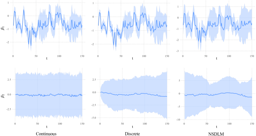
Figure 13. Two estimated slopes of each method. The solid lines and the shaded areas represent the posterior means and the 95% credible intervals, respectively.

References

- Alaimo Di Loro et al. [2023] Pierfrancesco Alaimo Di Loro, Marco Mingione, Jonah Lipsitt, Christina M Batteate, Michael Jerrett, and Sudipto Banerjee. Bayesian hierarchical modeling and analysis for actigraph data from wearable devices. The Annals of Applied Statistics, 17(4):2865 – 2886, 2023. doi: 10.1214/23-AOAS1742.
- Bai et al. [2018] Jiawei Bai, Yifei Sun, Jennifer A Schrack, Ciprian M Crainiceanu, and Mei-Cheng Wang. A two-stage model for wearable device data. Biometrics, 74(2):744–752, 2018.
- Banerjee et al. [2014] Sudipto Banerjee, Bradley P Carlin, and Alan E Gelfand. Hierarchical Modeling and Analysis for Spatial Data. Chapman and Hall/CRC, 2 edition, 2014. doi: 10.1201/b17115.
- Banker and Song [2023] Margaret Banker and Peter X. K. Song. Supervised learning of physical activity features from functional accelerometer data. IEEE Journal of Biomedical and Health Informatics, 27(12):5710–5721, 2023. doi: 10.1109/JBHI.2023.3318205.
- Bhatt et al. [2017] Samir Bhatt, Ewan Cameron, Seth R Flaxman, Daniel J Weiss, David L Smith, and Peter W Gething. Improved prediction accuracy for disease risk mapping using gaussian process stacked generalization. Journal of The Royal Society Interface, 14(134):20170520, 2017. doi: 10.1098/rsif.2017.0520.
- Blitzstein and Hwang [2019] Joseph K Blitzstein and Jessica Hwang. Introduction to Probability, Second Edition. Chapman and Hall/CRC, 2 edition, 2019. doi: 10.1201/9780429428357.
- Boyd and Vandenberghe [2004] Stephen Boyd and Lieven Vandenberghe. Convex Optimization. Cambridge University Press, 2004. doi: 10.1017/CBO9780511804441.
- Bürkner [2023] Paul-Christian Bürkner. brms: Bayesian Regression Models using ’Stan’, 2023. URL https://CRAN.R-project.org/package=brms. R package version 3.2.0.
- Carter and Kohn [1994] Chris K Carter and Robert Kohn. On Gibbs sampling for state space models. Biometrika, 81(3):541–553, 1994. doi: 10.1093/biomet/81.3.541.
- Chang and McKeague [2022] Hsin-wen Chang and Ian W McKeague. Empirical likelihood-based inference for functional means with application to wearable device data. Journal of the Royal Statistical Society Series B: Statistical Methodology, 84(5):1947–1968, 2022. doi: 10.1111/rssb.12543.
- Cressie and Huang [1999] Noel Cressie and Hsin-Cheng Huang. Classes of nonseparable, spatio-temporal stationary covariance functions. Journal of the American Statistical Association, 94(448):1330–1339, 1999.
- Cressie and Wikle [2015] Noel Cressie and Christopher K Wikle. Statistics for spatio-temporal data. John Wiley & Sons, 2015.
- Crouter et al. [2006] Scott E Crouter, Kurt G Clowers, and David R Bassett Jr. A novel method for using accelerometer data to predict energy expenditure. Journal of applied physiology, 100(4):1324–1331, 2006.
- Doherty et al. [2017] Aiden Doherty, Dan Jackson, Nils Hammerla, Thomas Plötz, Patrick Olivier, Malcolm H Granat, Tom White, Vincent T Van Hees, Michael I Trenell, Christoper G Owen, et al. Large scale population assessment of physical activity using wrist worn accelerometers: The uk biobank study. PloS one, 12(2), 2017.
- Durrett [2019] Rick Durrett. Probability: Theory and Examples. Cambridge Series in Statistical and Probabilistic Mathematics. Cambridge University Press, 5 edition, 2019.
- Freedson et al. [2012] Patty Freedson, Heather R Bowles, Richard Troiano, and William Haskell. Assessment of physical activity using wearable monitors: Recommendations for monitor calibration and use in the field. Medicine and science in sports and exercise, 44(1 Suppl 1):S1, 2012.
- Frühwirth-Schnatter [1994] Sylvia Frühwirth-Schnatter. Data augmentation and dynamic linear models. Journal of Time Series Analysis, 15(2):183–202, 1994. doi: https://doi.org/10.1111/j.1467-9892.1994.tb00184.x.
- Gamerman et al. [2008] Dani Gamerman, Hedibert Freitas Lopes, and Esther Salazar. Spatial dynamic factor analysis. Bayesian Analysis, 3(4):759 – 792, 2008. doi: 10.1214/08-BA329.
- Gelman et al. [2013] Andrew Gelman, John B. Carlin, Hal S. Stern, David B. Dunson, Aki Vehtari, and Donald B. Rubin. Bayesian Data Analysis. Chapman and Hall/CRC, 3 edition, 2013. doi: 10.1201/b16018.
- Ghosal and van der Vaart [2017] Subhashis Ghosal and Aad van der Vaart. Fundamentals of Nonparametric Bayesian Inference. Cambridge Series in Statistical and Probabilistic Mathematics. Cambridge University Press, 2017.
- Gneiting [2002] Tilmann Gneiting. Nonseparable, stationary covariance functions for space–time data. Journal of the American Statistical Association, 97(458):590–600, 2002.
- Goldfarb and Idnani [1983] Donald Goldfarb and Ashok Idnani. A numerically stable dual method for solving strictly convex quadratic programs. Mathematical Programming, 27:1–33, 1983. doi: 10.1007/BF02591962.
- Hoef and Peterson [2010] Jay M. Ver Hoef and Erin E. Peterson. A moving average approach for spatial statistical models of stream networks. Journal of the American Statistical Association, 105(489):6–18, 2010. doi: 10.1198/jasa.2009.ap08248.
- Hoef et al. [2006] Jay M. Ver Hoef, Erin E. Peterson, and David Theobald. Spatial statistical models that use flow and stream distance. Environmental and Ecological Statistics, 13:449–464, 2006. doi: 10.1007/s10651-006-0022-8.
- Hoeting et al. [1999] Jennifer A. Hoeting, David Madigan, Adrian E. Raftery, and Chris T. Volinsky. Bayesian model averaging: a tutorial (with comments by M. Clyde, David Draper and E. I. George, and a rejoinder by the authors. Statistical Science, 14(4):382 – 417, 1999. doi: 10.1214/ss/1009212519.
- Hooten et al. [2017] Mevin B Hooten, Devin S Johnson, Brett T McClintock, and Juan M Morales. Animal movement: statistical models for telemetry data. CRC press, 2017.
- Ishikawa-Takata et al. [2008] K Ishikawa-Takata, I Tabata, S Sasaki, HH Rafamantanantsoa, H Okazaki, H Okubo, S Tanaka, S Yamamoto, T Shirota, K Uchida, et al. Physical activity level in healthy free-living japanese estimated by doubly labelled water method and international physical activity questionnaire. European Journal of Clinical Nutrition, 62(7):885–891, 2008.
- James et al. [2016] Peter James, Marta Jankowska, Christine Marx, Jaime E. Hart, David Berrigan, Jacqueline Kerr, Philip M. Hurvitz, J. Aaron Hipp, and Francine Laden. “spatial energetics”: Integrating data from gps, accelerometry, and gis to address obesity and inactivity. American Journal of Preventive Medicine, 51(5):792–800, 2016. doi: 10.1016/j.amepre.2016.06.006.
- Jurek et al. [2023] Marcin Jurek, Catherine A Calder, and Corwin Zigler. Statistical inference for complete and incomplete mobility trajectories under the flight-pause model. Journal of the Royal Statistical Society Series C: Applied Statistics, 73(1):162–192, 11 2023. doi: 10.1093/jrsssc/qlad090.
- Lange [2010] Kenneth Lange. Numerical Analysis for Statisticians. Springer New York, 2010. doi: 10.1007/978-1-4419-5945-4.
- Le and Clarke [2017] Tri Le and Bertrand Clarke. A Bayes Interpretation of Stacking for -Complete and -Open Settings. Bayesian Analysis, 12(3):807 – 829, 2017. doi: 10.1214/16-BA1023.
- Li et al. [2023] Didong Li, Wenpin Tang, and Sudipto Banerjee. Inference for gaussian processes with matern covariogram on compact riemannian manifolds. Journal of Machine Learning Research, 24(101):1–26, 2023.
- Luo et al. [2023] Lan Luo, Jingshen Wang, and Emily C Hector. Statistical inference for streamed longitudinal data. Biometrika, 110(4):841–858, 02 2023. ISSN 1464-3510. doi: 10.1093/biomet/asad010.
- Lyden et al. [2014] Kate Lyden, Sarah Kozey Keadle, John Staudenmayer, and Patty S Freedson. A method to estimate free-living active and sedentary behavior from an accelerometer. Medicine and science in sports and exercise, 46(2):386, 2014.
- Mohri et al. [2018] Mehryar Mohri, Afshin Rostamizadeh, and Ameet Talwalkar. Foundations of machine learning. MIT press, 2 edition, 2018.
- Murphy [2023] Kevin P. Murphy. Probabilistic Machine Learning: Advanced Topics. MIT Press, 2023.
- Peña and Poncela [2004] Daniel Peña and Pilar Poncela. Forecasting with nonstationary dynamic factor models. Journal of Econometrics, 119(2):291–321, 2004. doi: https://doi.org/10.1016/S0304-4076(03)00198-2.
- Phillips et al. [2019] T.R.L. Phillips, K.M. Schmidt, and A. Zhigljavsky. Extension of the schoenberg theorem to integrally conditionally positive definite functions. Journal of Mathematical Analysis and Applications, 470(1):659–678, 2019. doi: https://doi.org/10.1016/j.jmaa.2018.10.032.
- Prado et al. [2021] Raquel Prado, Marco A. R. Ferreira, and Mike West. Time Series: Modeling, Computation, and Inference. Chapman and Hall/CRC, 2 edition, 2021. doi: 10.1201/9781351259422.
- R Core Team [2024] R Core Team. R: A Language and Environment for Statistical Computing. R Foundation for Statistical Computing, Vienna, Austria, 2024. URL https://www.R-project.org/.
- Robert and Casella [2004] Christian P Robert and George Casella. Monte Carlo Statistical Methods. Springer New York, 2 edition, 2004. doi: 10.1007/978-1-4757-4145-2.
- Rue et al. [2009] Håvard Rue, Sara Martino, and Nicolas Chopin. Approximate bayesian inference for latent gaussian models by using integrated nested laplace approximations. Journal of the Royal Statistical Society: Series B: Statistical Methodology, 71(2):319–392, 2009. doi: https://doi.org/10.1111/j.1467-9868.2008.00700.x.
- Santos-Fernandez et al. [2022] Edgar Santos-Fernandez, Jay M. Ver Hoef, Erin E. Peterson, James McGree, Daniel J. Isaak, and Kerrie Mengersen. Bayesian spatio-temporal models for stream networks. Computational Statistics & Data Analysis, 170:107446, 2022. doi: https://doi.org/10.1016/j.csda.2022.107446.
- Spiegelhalter et al. [2002] David J Spiegelhalter, Nicola G Best, Bradley P Carlin, and Angelika Van Der Linde. Bayesian measures of model complexity and fit. Journal of the Royal Statistical Society Series B: Statistical Methodology, 64(4):583–639, 2002. doi: https://doi.org/10.1111/1467-9868.00353.
- Staudenmayer et al. [2015] John Staudenmayer, Shai He, Amanda Hickey, Jeffer Sasaki, and Patty Freedson. Methods to estimate aspects of physical activity and sedentary behavior from high-frequency wrist accelerometer measurements. Journal of applied physiology, 119(4):396–403, 2015.
- Stein [1999] Michael L Stein. Interpolation of Spatial Data: Some Theory for Kriging. Springer New York, 1999. doi: 10.1007/978-1-4612-1494-6.
- Stein [2005] Michael L Stein. Space–time covariance functions. Journal of the American Statistical Association, 100(469):310–321, 2005.
- Stroud et al. [2001] Jonathan R. Stroud, Peter Müller, and Bruno Sansó. Dynamic models for spatiotemporal data. Journal of the Royal Statistical Society Series B: Statistical Methodology, 63(4):673–689, 2001. doi: https://doi.org/10.1111/1467-9868.00305.
- Tang et al. [2021] Wenpin Tang, Lu Zhang, and Sudipto Banerjee. On Identifiability and Consistency of The Nugget in Gaussian Spatial Process Models. Journal of the Royal Statistical Society Series B: Statistical Methodology, 83(5):1044–1070, 2021. doi: 10.1111/rssb.12472.
- Taraldsen et al. [2012] Kristin Taraldsen, Sebastien FM Chastin, Ingrid I Riphagen, Beatrix Vereijken, and Jorunn L Helbostad. Physical activity monitoring by use of accelerometer-based body-worn sensors in older adults: A systematic literature review of current knowledge and applications. Maturitas, 71(1):13–19, 2012.
- Turlach and Weingessel [2019] Berwin A. Turlach and Andreas Weingessel. quadprog: Functions to Solve Quadratic Programming Problems, 2019. URL https://CRAN.R-project.org/package=quadprog. R package version 1.5-8.
- van der Laan et al. [2007] Mark J. van der Laan, Eric C Polley, and Alan E. Hubbard. Super learner. Statistical Applications in Genetics and Molecular Biology, 6(1), 2007. doi: doi:10.2202/1544-6115.1309.
- Watanabe [2010] Sumio Watanabe. Asymptotic equivalence of bayes cross validation and widely applicable information criterion in singular learning theory. Journal of Machine Learning Research, 11(116):3571–3594, 2010.
- West and Harrison [1997] Mike West and Jeff Harrison. Bayesian Forecasting and Dynamic Models. Springer New York, 2 edition, 1997. doi: 10.1007/0-387-22777-6.
- Yao et al. [2018] Yuling Yao, Aki Vehtari, Daniel Simpson, and Andrew Gelman. Using Stacking to Average Bayesian Predictive Distributions (with Discussion). Bayesian Analysis, 13(3):917 – 1007, 2018. doi: 10.1214/17-BA1091.
- Zhang [2004] Hao Zhang. Inconsistent estimation and asymptotically equal interpolations in model-based geostatistics. Journal of the American Statistical Association, 99(465):250–261, 2004. doi: 10.1198/016214504000000241.
- Zhang et al. [2023] Lu Zhang, Wenpin Tang, and Sudipto Banerjee. Exact bayesian geostatistics using predictive stacking. arXiv preprint arXiv:2304.12414, 2023.