Density-based clustering algorithm for galaxy group/cluster identification

Abstract

A direct approach to studying the galaxy-halo connection is the analysis of observed groups and clusters of galaxies that trace the underlying dark matter halos, making identifying galaxy clusters and their associated brightest cluster galaxies (BCGs) crucial. We test and propose a robust density-based clustering algorithm that outperforms the traditional Friends-of-Friends (FoF) algorithm in the currently available galaxy group/cluster catalogs. Our new approach is a modified version of the Ordering Points To Identify the Clustering Structure (OPTICS) algorithm, which accounts for line-of-sight positional uncertainties due to redshift space distortions by incorporating a scaling factor, and is thereby referred to as sOPTICS. When tested on both a galaxy group catalog based on semi-analytic galaxy formation simulations and observational data, our algorithm demonstrated robustness to outliers and relative insensitivity to hyperparameter choices. In total, we compared the results of eight clustering algorithms. The proposed density-based clustering method, sOPTICS, outperforms FoF in accurately identifying giant galaxy clusters and their associated BCGs in various environments with higher purity and recovery rate, also successfully recovering 115 BCGs out of 118 reliable BCGs from a large galaxy sample.

1 Introduction

Galaxy groups are fundamental structures in the universe comprising multiple galaxies bound together by gravity within a dark matter halo (White & Rees, 1978). Galaxies in a group are located near the peak of this dark matter density distribution, where the gravitational potential is deepest (Moore et al., 1998; Thanjavur et al., 2010; Shin et al., 2022). More numerous aggregations of galaxies are classified as clusters of galaxies, composed of hundreds to thousands of galaxies, hot gas, and predominantly dark matter. Galaxy groups and clusters are key components in understanding the formation of hierarchical structures in the universe, especially since they are closely related to dark matter halos.

Therefore, identifying groups and clusters of galaxies is a crucial step in understanding the distribution and evolution of matter in the universe. The study of galaxy groups and clusters has been an active field of research for decades, with various methods developed for identifying and characterizing these structures.

In addition, central to galaxy clusters are the Brightest Cluster Galaxies (BCGs) located at the bottom of gravitational well within the clusters (Quintana & Lawrie, 1982). The properties of BCGs dictate cluster formation and evolution, where BCG mass growth is closely tied to the hierarchical assembly and dynamical state of the host galaxy cluster (Sohn et al., 2021). What is more distinct from other galaxies is that some of the BCGs show multiple nuclei (e.g. Lauer, 1988; Kluge et al., 2020), making them good systems to study about galactic mergers. A recent study on velocity dispersion profiles of elliptical galaxies also found the majority of the BCGs exhibit flat velocity dispersion profiles (Tian et al., 2021; Duann et al., 2023). A distinct radial acceleration relation (RAR) has even been identified in BCGs, making them essential by posing a significant challenge to the cold dark matter (CDM) paradigm (Tian et al., 2024). However, identifying BCGs can be complex, often requiring a comprehensive survey of galaxies and coherently identifying a pure and complete galaxy clusters catalog first.

To effectively identify galaxy groups, we need to identify denser regions within a sparse distribution of galaxies. This approach resembles finding concentrated islands amid a vast, sparse ocean. Traditionally, the foundation of clustering algorithms has been based on the single-link clustering methodology. A quintessential example of this approach is the Friends-of-Friends (FoF; Turner & Gott, 1976; Huchra & Geller, 1982; Press & Davis, 1982; Tago et al., 2008) algorithm. The FoF method links galaxies within a specified proximity, progressively forming clusters. Single-link clustering generally results in clusters where even distantly related members are interconnected through a sequence of nearer members, leading to the term "single-link". However, this method is sensitive to noise, where an isolated noisy data point might erroneously connect neighbor clusters, leading to the merging of clusters that are otherwise distinct, compromising the accuracy of the clustering results. Additionally, this approach can yield clusters with a chain-like configuration, which is highly sensitive to the predefined linking length, a hyperparameter. Nevertheless, despite these limitations, single-link clustering remains a valuable tool due to its efficiency and simplicity, particularly for identifying groups and clusters of stars or galaxies with elongated or irregular shapes (Sankhyayan et al., 2023; Chi et al., 2023).

Density-based clustering methodologies, such as the Density-Based Spatial Clustering of Applications with Noise (DBSCAN; Ester et al., 1996; Sander et al., 1998), have been introduced to address these limitations and enhance the robustness of cluster identification. These methods rely on estimating the density of data points, allowing for separation between lower-density areas and higher-density regions. The primary aim here is not to distinctly separate these two areas but to enhance the robustness of the identified core clusters against noise. By doing so, these algorithms provide a more reliable means of cluster identification, which is crucial in analyzing galaxy distributions. Therefore, density-based clustering algorithms for identifying galaxy groups have emerged as alternatives to FoF. DBSCAN identifies clusters based on the density of points, designating core points with a high density of neighbors and expanding clusters from these cores. This method effectively lowers the influence of isolated noise points, thus making the identification of clusters of points more robust and reflective of the true spatial distribution. Its effectiveness is particularly notable for discovering open clusters of stars (Castro-Ginard et al., 2018, 2020) as well as clusters and groups of galaxies (Dehghan & Johnston-Hollitt, 2014; Olave-Rojas et al., 2023).

However, DBSCAN has limitations, particularly in handling datasets with varying density clusters. Since it relies on a single density threshold to define clusters, DBSCAN can struggle to effectively identify clusters of varying densities. To address these shortcomings, algorithms like Hierarchical Density-Based Spatial Clustering of Applications with Noise (HDBSCAN; Campello et al., 2015; McInnes et al., 2017) and Ordering Points To Identify the Clustering Structure (OPTICS; Ankerst et al., 1999) have been introduced. In these algorithms, dense points remain the same distance with each other, but noise points are pushed away from any other point. This effectively ‘lowers the sea level’ spreading sparse ‘sea’ points out while leaving ‘land’ untouched. These enhancements make HDBSCAN and OPTICS more suitable for identifying clusters and groups of stars and galaxies that more closely resemble the real distribution and density variations them (Brauer et al., 2022; Fuentes et al., 2017; Oliver et al., 2021).

Since BCGs are typically located at the bottom of the gravitational well, often indicating the densest region of a galaxy cluster, density-based clustering methods are anticipated to be particularly effective for identifying BCGs, even in complex and noisy environments. This effectiveness arises from the inherent capability of these methods to concentrate on the most dense regions, provided that the corresponding hyperparameters are set appropriately to define BCGs. In contrast, the FoF algorithm may struggle with clustering galaxies upon varying density. This is because its criteria for linking galaxies do not rely on density but on proximity, which might not accurately reflect the underlying density variations, especially in identifying BCGs.

Therefore, in this work, we conduct comprehensive tests on various clustering methods to explore the possibilities and challenges of identifying galaxy groups and clusters from large galaxy surveys and propose a new algorithm. This paper is organized as follows: Section 2 provides a concise introduction to the clustering algorithms used in this study, detailing the methodology for feature extraction and hyperparameter optimization, including the selection criteria. Section 3 offers a comprehensive evaluation of the effectiveness of group finders using a galaxy catalog derived from simulations. Following this, Section 4 presents additional tests conducted with real-world observations, which include mitigating redshift space distortion using our proposed line-of-sight scaling factor and comparisons with a reliable group catalog. Section 5.1 discusses the strength of our sOPTICS method and its efficiency in identifying BCGs. Finally, Section 6 summarizes our findings and provides a detailed discussion of the results.

2 Clustering Methodology

Clustering, a technique in machine learning, groups similar data points into clusters and is a powerful tool for identifying galaxy groups in astronomical data. Determining the most advanced clustering algorithm in data science is challenging, as it largely depends on the specific use case and data type. Importantly, a more advanced algorithm is not necessarily a better fit for every dataset or task. This consideration is crucial when employing these algorithms for practical applications, such as extracting galaxy groups and clusters from observations. Hence, an algorithm should be selected based on its suitability for the specific problem. In our research, we have applied eight different clustering algorithms to the 3D spatial positions of simulated galaxies in comoving space. These algorithms include $k$-means (MacQueen, 1967), Gaussian Mixture Models (GMMs) (Dempster et al., 1977), Spectral Clustering (Ng et al., 2001; von Luxburg, 2007), Agglomerative Clustering (Ward, 1963), as well as FoF, DBSCAN, HDBSCAN, and OPTICS, as introduced in Section 1. First, we briefly describe each of these algorithms below.

2.1 Clustering Algorithms

Among all the clustering algorithms considered here, $k$-means stands out for its simplicity of implementation and computational efficiency. The core principle behind $k$-means is to minimize the total intra-cluster variance by constructing clusters and their corresponding centroids. However, traditional $k$-means and its variants are susceptible to local minima in the minimum-sum-of-squares objective function (Bottou & Bengio, 1994). This implies that the clustering result for a given dataset may vary depending on the randomly initialized centroids, impacting the overall process. Consequently, while computationally inexpensive, $k$-means is often utilized as a starting point for computationally heavier algorithms, such as GMMs.

GMMs are generative models capable of representing data with multiple underlying modes or clusters as a linear combination of weighted Gaussian distributions. GMMs are well-suited for soft clustering tasks, where each data point can belong to multiple clusters with varying degrees of membership represented by probabilities. However, GMMs generally require more iterations of the expectation–maximization (EM) algorithm (Dempster et al., 1977) to converge compared to $k$-means, resulting in slower execution times.

Spectral clustering operates under the principle of graph partitioning. It first constructs a similarity graph where nodes represent data points and edges represent similarities between them. Then, it analyzes the eigenvectors (spectrum) of the Laplacian matrix of the Laplacian matrix of this graph to project the data into a lower-dimensional space where traditional clustering algorithms (e.g., $k$-means) can be performed. This approach allows spectral clustering to excel in identifying clusters not linearly separable in the original data space.

Agglomerative clustering employs a bottom-up approach, progressively merging clusters based on their proximity. In this work, we choose the Ward linkage method (Ward, 1963), which minimizes the total within-cluster variance. At each step, the pair of clusters with the minimum between-cluster distance are merged, leading to clusters that are internally coherent and well-separated from each other.

The FoF algorithm is the most popular way of identifying galaxy clusters within a cosmic structure. Given a set of points in space, the FoF algorithm links points within a predetermined distance $l$ to identify interconnected clusters. Two points are considered ‘friends’ (i.e., part of the same cluster) if they are within $l$ of each other. This process iteratively groups points together by linking points to their friends and friends of friends.

The last three algorithms, DBSCAN, HDBSCAN, and OPTICS, are all density-based clustering algorithms. For each point in the dataset, DBSCAN calculates the number of points within a specified radius $\epsilon$. If this number exceeds a minimum number of neighbors $N_{\mathrm{min}}$, the point is classified as a core point, indicating a high-density area surrounding it. The core distance $d_{\mathrm{core}}$ is the minimum radius of a neighborhood around this point that must contain a certain number of other points to qualify the point as a core point. These core points serve as the seeds for cluster growth, as the algorithm iteratively adds directly reachable points (points located within the $\epsilon$-radius of a core point) to their respective clusters. Points not reachable from any core point are labeled as noise.

HDBSCAN, on the other hand, builds upon DBSCAN’s concept but introduces a hierarchy of clusters. It first estimates the density of each point using the mutual reachability distance,

$$d_{\mathrm{reach}}(P,Q)=\max\{d_{\mathrm{core}}(P,N_{\mathrm{min}}),d(P,Q)\}\,,$$ (1)

where $d(P,Q))$ is the Euclidean distance between two points. HDBSCAN then constructs a minimum spanning tree (MST: e.g., Foulds 1991), which connects all data points in a way that the total sum of edge lengths (distances) is minimized. By systematically removing the longest edges from the MST, HDBSCAN creates a dendrogram that reflects the data structure at varying density levels. Each cluster’s stability is calculated as the sum of the excess of density (over a minimum cluster size threshold) for each point within the cluster across the range of distance scales. Finally, HDBSCAN iteratively prunes this dendrogram using the stability criterion, resulting in robust and persistent clusters over a range of densities. (Campello et al., 2013)

Instead of a global $\epsilon$ parameter, OPTICS uses reachability to create an ordered list reflecting the data structure. This ordered list is constructed by iteratively updating the reachability distance for each data point. Starting with an arbitrary point, its reachability distance is calculated relative to its neighbors. This point is added to the list, and the algorithm progresses to the unprocessed point with the smallest reachability distance. This process continues until all points are ordered. This resulting list effectively captures the density-based clustering structure without explicitly assigning points to clusters. Clusters can be extracted by identifying valleys (i.e., low reachability distance regions indicating dense areas) separated by peaks (i.e., high reachability distances marking transitions between clusters or noise). In practice, the $\xi$ parameter defines what constitutes a "steep" decrease or increase: a point is part of a steep downward (or upward) area if its reachability distance is less (or greater) than $\xi$ times the reachability distance of the preceding point in the ordered list.

2.2 Hyperparameter Optimization

Hyperparameter selection for each of the algorithms in our task requires careful consideration, including the characteristics of the target groups or clusters, data resolution, and noise levels. The following is a breakdown of key hyperparameters for each method.

$k$-means, GMM, Spectral Clustering, and Agglomerative Clustering all share the critical hyperparameter of the number of clusters, $N_{\mathrm{C}}$. Finding the optimal $N_{\mathrm{C}}$ requires careful consideration of the data complexity and desired level of cluster granularity. The FoF method critically relies on the linking length, $l_{\mathrm{linking}}$ to define the scale at which structures are identified.

For DBSCAN, the two primary hyperparameters are $N_{\mathrm{min}}$ and $\epsilon$, which control the degree to which a point is considered a core point. Higher $\epsilon$ values incorporate distant galaxies into clusters, facilitating the identification of larger groups but potentially over-grouping due to projection effects. Conversely, a higher $N_{\mathrm{min}}$ threshold helps identify more significant clusters, reducing the possibility of detecting spurious or minor groupings. HDBSCAN relies on an additional layer of complexity with the min_cluster_size parameter ($M_{\mathrm{min}}$). This parameter sets the minimum number of members required for a grouping to be considered a valid cluster, allowing for the filtering of insignificant or noisy structures. Besides, there is an additional hyperparameter $\alpha$, which relates to the minimum cluster stability required for a cluster to be considered significant. A lower value of $\alpha$ makes it easier for points to be included in a cluster, potentially leading to larger and less dense clusters.

In the case of OPTICS, there are four key hyperparameters, with $N_{\mathrm{min}}$ and $\epsilon$ exerting the most influence. Beyond these two, the $\xi$ parameter plays a crucial role, with lower values leading to the identification of more clusters, even capturing subtle variations in galaxy density. This sensitivity is advantageous for distinguishing closely spaced or subtly different groups. Finally, the minimum number of member galaxies per group, $M_{\mathrm{min}}$, is a straightforward parameter set based on the desired group scale. In the following tests and results, we set $M_{\mathrm{min}}=5$ to focus on groups with at least five members.

All clustering algorithms in this work require a preselected hyperparameter carefully considered for the desired galaxy group scale. Choosing the optimal hyperparameter values involves balancing the preservation of large-scale structures against the fragmentation of real galaxy groups into smaller, potentially insignificant groups. To optimize hyperparameter values, we adopted two classical criteria, purity and completeness, to evaluate the performance of clustering algorithms under different hyperparameter settings. However, comparing results to a simulated group catalog introduces inherent biases. Simulations, while valuable, are not perfect representations of real galaxy groups, and even semi-analytic galaxy group catalogs are usually constructed using FoF clustering algorithms (Onions et al., 2012, also see Section 3.1), introducing bias in the "ground truth" data. Consequently, demanding complete overlap between predicted and simulated groups is unrealistic and unnecessary. Instead, similar to Brauer et al. (2022), we define a broader measure of purity and completeness, incorporating what we term as soft criteria, to assess the performance of the clustering algorithms for a more nuanced evaluation. Under these criteria, a cluster is considered pure if at least two-thirds of its galaxies originated from a single group and complete if it contains at least half the galaxies from that originating group. Building upon the definitions of purity and completeness, we can define the purity rate and recovery rate for all predicted groups relative to the full set of true groups:

$$F_{\mathrm{P}}=\frac{\text{Number of pure groups}}{\text{Total number of predicted groups}}\,,$$ (2)

$$F_{\mathrm{R}}=\frac{\text{Number of simultaneously pure and complete groups}}{\text{Total number of true groups}}\;.$$ (3)

When calculating purity and recovery rates, we only compare predicted groups to true groups exceeding the minimum member threshold, $M_{\mathrm{min}}$=5. It is worth noting that, to calculate purity, the traversal list here is all the predicted groups, not the halo IDs in the simulation catalog. Meanwhile, to calculate the recovery rate, the traversal list is all the halos with at least $M_{\mathrm{min}}$ galaxy members in the simulation catalog rather than the predicted groups. Consequently, the purity rate reflects the proportion of predicted groups exclusively containing members from a single true group. It provides confidence for ensuring that the members within a predicted group are genuinely bound together. A high purity rate indicates that the algorithm is effective in correctly grouping members. On the other hand, the recovery rate measures the percentage of true, significant groups successfully identified and reproduced by the algorithm. This ensures the informativeness and reliability of the results for further analysis.

We define search spaces of approximately 20 trial values for each hyperparameter to explore the impact of various hyperparameter choices. We then execute the clustering algorithm with each set of trial values and calculate purity and recovery rates (see Section 3). The optimal hyperparameter values for each algorithm are chosen by maximizing the recovery rate. In cases where multiple sets yield the same recovery rate, the set with the highest purity rate is preferred. Table 1 provides an overview of the trial hyperparameter values and the optimized results against the simulated group catalog.

3 Tests with simulated group catalog

A crucial test of any group finder’s performance involves comparing its results to the expected distribution of galaxies in a group catalog built from simulations using semi-analytic models (SAMs, Kauffmann & Haehnelt, 2000; Springel et al., 2001). This allows us to assess how well the group finder aligns with the theoretical framework of galaxy formation. In this work, we utilize a galaxy group catalog (Croton et al., 2006; De Lucia & Blaizot, 2007) built from The Millennium Simulation (Springel et al., 2005), which provides a well-established and widely used benchmark for testing group finder performance.

3.1 Galaxy Sample

The Millennium Simulation tracks the evolution of $N=2160^{3}$ dark matter particles within a comoving volume of $500\,\mathrm{h}^{-1}\mathrm{Mpc}$ using the N-body code GADGET-2 (Springel, 2005). Sixty-four snapshots were periodically saved, along with group catalogs and their substructures identified through a two-step process. First, the FoF algorithm with a linking length of 0.2 in units of the mean particle separation identified potential halos. These candidates were then refined by the SUBFIND algorithm (Springel et al., 2001) through a gravitational unbinding procedure, ensuring only substructures with at least 20 particles were considered to be genuine halos and substructures. Subsequently, with halos detailed merger history trees were constructed for all gravitationally bound structures in each snapshot. The merger trees trace the evolution of these structures throughout cosmic time, providing the crucial temporal and structural framework upon which SAMs operate. Within this framework, SAMs simulate the formation and evolution of galaxies, ultimately populating the dark matter halos with galaxies. (De Lucia & Blaizot, 2007)

From the semi-analytic galaxy group catalogs of De Lucia & Blaizot (2007), we extracted a cubic sub-volume of $50\,\mathrm{h}^{-1}\mathrm{Mpc}$ side length at snapshot 63 (corresponding to redshift $z=0$) as our fiducial test sample. This sub-volume contains 26,276 galaxies originating from 17,878 halos. However, most of these halos only host a single galaxy, making them unsuitable for characterizing groups or clusters. Therefore, we focused on halos containing at least five galaxies, resulting in a final sample of 400 halos. We further expanded our analysis by extracting similar sub-volumes at snapshots 30 ($z=2.422$), 40 ($z=1.078$), and 50 ($z=0.408$) to explore the performance of the clustering algorithms across different cosmic epochs. It is important to note that our analysis is restricted to real space (3D Cartesian coordinates) for computational efficiency, neglecting the effects of peculiar velocities and, consequently, redshift-space distortions.

3.2 Comparing Clustering Algorithms

Considering the hierarchical structure of the Universe, with galaxy groups typically hosting 3 to 30 bright galaxies and clusters holding 30 to over 300, it is logical to focus our search for optimal clustering parameters within this range. The Local Group, for instance, hosts over 30 galaxies with a diameter of nearly 3 Mpc (McConnachie et al., 2005). Therefore, we set the searching space of distance thresholds for clustering algorithms between 0.1 Mpc and a few Mpc. Similarly, the minimum neighbor number $N_{\mathrm{min}}$ and minimum member number $M_{\mathrm{min}}$ are explored within the range of 2-20. We employ a broader range, 500 to 5000, for algorithms requiring a preselected number of clusters, to ensure exploring all possibilities. The trial hyperparameter values for all algorithms are listed in Table 1.

We apply the eight algorithms described in Section 2 to the test sample obtained in Section 3.1, evaluating each algorithm with all trial hyperparameter values. The python package GalCluster we developed to conduct the tests is realized. This tool lets users easily perform galaxy group finding on a simulated observed catalog. We calculate the purity and recovery rates for each run according to the soft criteria by comparing the predicted groups with the true halo IDs in the simulation. We subsequently select the optimal hyperparameters that maximize the recovery rate. The complete results, including the predicted groups corresponding to the optimal hyperparameters, are presented in Table 1.

Algorithm	Hyperparameter	Search space	Optimal Value	Maximum recovery rate	Number of groups
Friend-of-friends	linking_length $l$	[0.001, 3.0)	0.18	83.5%	1114
	max_eps $\epsilon$	[0.05, 1.0)	0.2
OPTICS	min_sample $N_{\mathrm{min}}$	[2, 20)	3	83.0%	1035
	xi $\xi$	[0.05, 1.0)	0.95
	min_member $M_{\mathrm{min}}$	[2, 20)	3
DBSCAN	max_eps $\epsilon$	[0.05, 1.0)	0.2
	min_sample $N_{\mathrm{min}}$	[2, 20)	2	84.0%	2778
	min_member $M_{\mathrm{min}}$	[2, 20)	2
	min_sample $N_{\mathrm{min}}$	[2, 20)	2
HDBSCAN	min_member $M_{\mathrm{min}}$	[2, 20)	2	54.5%	3433
	alpha $\alpha$	[0.05, 1]	0.90
$k$-means			>5000	54.7%	5000
GMM	n_clusters $N_{\mathrm{C}}$	[500, 5000)	>5000	7.6%	5000
Agglomerative Clustering			>5000	57.3%	5000
Spectral Clustering			too slow	-	-

Table 1: Trial hyperparameter values for all algorithms and the best fitting values to maximize the recovery rate under soft criteria, respectively. Note that since the processing time for GMM, $k$-means, Agglomerative Clustering, and Spectral Clustering on the test sample are very long, and Iterating them over the searching space takes even more time, we hereby adopt a subsample for fitting their hyperparameters.

As we can see from the results, the traditional methods FoF, OPTICS, and DBSCAN can effectively recover the galaxy groups just based on the spatial distribution of galaxies with a recovery rate of over 70%. The others can not give a good prediction of the groups. It should also be emphasized that the ground was calculated based on the FoF algorithm.

3.3 Parameter Sensitivity

Even though FoF and OPTICS are comparable in predicting galaxy groups, they differ significantly in their hyperparameter complexities. OPTICS requires tuning four hyperparameters, providing more flexibility and necessitating more careful configuration. On the other hand, FoF has only one primary hyperparameter, simplifying its use but potentially limiting its adaptability. This contrast raises questions about the sensitivity of their respective hyperparameters. To investigate this, purity, completeness, and recovery rates were calculated for each algorithm under different values of a single hyperparameter while keeping the others constant. Figure 1 presents results based on soft criteria. These analyses were conducted on the same subsample described in Section 3.1.

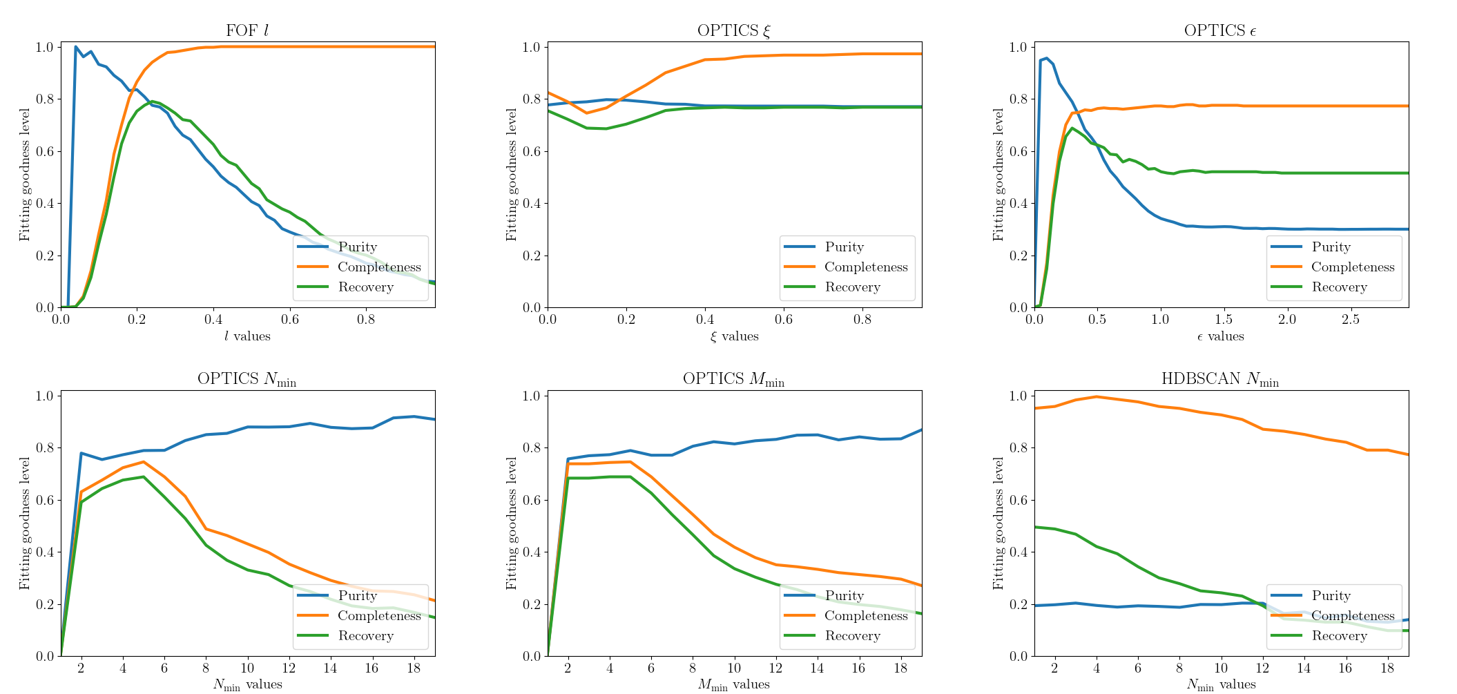
Figure 1: Results of parameter sensitivity tests conducted for the clustering algorithms FoF, HDBSCAN, and OPTICS, respectively. The metrics used to evaluate these tests were purity, completeness, and recovery rate, which were calculated by comparing the algorithms’ outputs with group catalogs derived from the Millennium Simulation.

Our analysis reveals that the FoF algorithm exhibits significant sensitivity to the linking length parameter over this hyperparameter’s entire possible value range. This dependency underscores the importance of careful tuning of the linking length parameter to ensure reliable identification of galaxy groups using the FoF method.

In comparison, the OPTICS results are primarily influenced by the minimum number of members $M_{\mathrm{min}}$ and minimum number of neighbors $N_{\mathrm{min}}$ parameters. Although the choice of $M_{\mathrm{min}}$ and $N_{\mathrm{min}}$ significantly affects the OPTICS results, it is noteworthy that setting these parameters to small values, such as in the range of 2 to 5, can achieve high completeness and purity in identifying galaxy groups and clusters. Increasing these parameters does not adversely affect the purity of the identified groups but only may reduce completeness. Consequently, choosing small values for $M_{\mathrm{min}}$ and $N_{\mathrm{min}}$ can be an appropriate strategy in the context of galaxy group and cluster identification, as it enables the algorithm to detect as many groups as possible from the entire data survey, including those with only a few members. Conversely, choosing larger values for $M_{\mathrm{min}}$ and $N_{\mathrm{min}}$ enables the focus on giant clusters, enhancing confidence in their identification.

As for the other two parameters of OPTICS, conventionally, the $\epsilon$ parameter primarily drives OPTICS results because, by definition, points lacking sufficient neighbors within an $\epsilon$-radius are classified as isolated, which is crucial for noise identification. However, surprisingly, the results exhibit remarkable stability for $\epsilon$ values exceeding 1.0, and even extreme choices still yield similar outcomes. This robustness can be attributed to how OPTICS extracts clusters from the reachability plot, where $\xi$ plays a dominant role. For $\epsilon$ values in a proper range, $\xi$ has less effect on clustering results, as depicted in Figures 1. This is because, in astronomical data, where galaxy groups and clusters are often more spatially distinct and less densely packed than objects in other types of datasets (like social networks or biological data), the natural separation between groups or clusters is already pronounced, reducing the need for fine-tuning $\xi$.

Finally, while HDBSCAN demonstrates low sensitivity to hyperparameter choices, its group prediction accuracy falls short, excluding its further consideration in this work.

In addition, it is noteworthy that extreme values of $\epsilon$ and $N_{\text{min}}$ in the OPTICS algorithm can achieve purity rates as high as 100%. This feature of OPTICS highlights its capacity to precisely and effectively identify the densest regions within galaxy clusters. Furthermore, this insight indicates a new approach to locating BCGs efficiently. The detection and analysis of BCGs are crucial for understanding the mass distribution in clusters and the evolutionary dynamics involved. In Section 5.1, we will explore the application of this method for BCG identification, evaluating its efficiency and broader implications.

4 Test with real-world group catalog

In Section 3, we have demonstrated the efficacy of the OPTICS algorithm, particularly highlighting its stability in parameter sensitivity tests compared to the FoF method. Nonetheless, applying to real observational data remains a unique challenge not encountered in simulations. For instance, the number density distribution of astronomical objects is significantly constrained by the limitations inherent to telescopes and surveys, as well as by environmental factors and redshift variations. A particularly critical issue that cannot be overlooked is the redshift-space distortion, which introduces complexities not accounted for in simulation-based analyses. Various models have been proposed to investigate redshift-space distortions in galaxy surveys. These include the Eulerian dispersion model (Kaiser, 1987), the Lagrangian perturbation model (Buchert, 1992; Bouchet et al., 1995) and the Gaussian streaming model (Reid & White, 2011; Reid et al., 2012), along with their variations. These models, including dispersion models and those expressing the redshift-space correlation function as an integral of the real-space correlation function, have been tested in configuration space to understand their predictive capabilities. It is shown that some models fitting simulations well over limited scales (on scales above $25-30\,h^{-1}$ Mpc) but failing at smaller scales (White et al., 2015). This limitation poses challenges in accurately correcting the identification of galaxy groups and clusters, typically smaller in scale. The random velocities of galaxies in groups and clusters contribute significantly to redshift-space distortions on small scales, impacting the precision of these models in correcting for such distortions (Marulli et al., 2017).

Consequently, extrapolating conclusions derived from simulations to real observational contexts requires caution. To address this, our research extends into the empirical evaluation of the FoF and OPTICS algorithms with real-world observational data of galaxies and galaxy groups, considering the effects of redshift-space distortions.

4.1 Data Sample

To conduct the evaluation of FoF and OPTICS on real-world observations, we adopt data from the seventh Sloan Digital Sky Survey (SDSS DR7; Abazajian et al., 2009). More specifically, we make use of the New York University Value-Added Galaxy Catalog (NYU-VAGC; Blanton et al., 2005), which is based on SDSS DR7 but includes a set of significant improvements over the original pipelines. We select all galaxies in the main galaxy sample from this catalog using the identical selection criteria described in Yang et al. (2007). This leaves 639,359 galaxies with reliable r-band magnitudes and measured redshifts from the SDSS DR7.

For our comparative analysis, we utilize the group and cluster catalog by Yang et al. (2007, hereafter Y07), updated to the version incorporating data from SDSS DR7 as a foundational reference. Among the three versions of group catalogs provided in Y07, we adopt the one that is constructed using the SDSS model magnitude and includes additional SDSS galaxies with redshifts from alternative sources. The selection of the group centers, which are also BCG candidates, in this catalog is based on luminosity, as detailed by Yang et al. (2005) in Section 3.2.

4.2 Cure the Redshift-Space Distortion via sOPTICS with a LOS Scaling Factor

As mentioned at the beginning of this section, one unavoidable challenge arises before applying OPTICS to real observations. Due to the redshift-space distortion phenomenon, galaxy groups exhibit an elongated appearance along the line of sight when observed in Cartesian coordinates (see Figure 2). When applied in a three-dimensional space, this elongation presents a significant challenge for clustering algorithms, such as OPTICS. Specifically, it results in an underestimation of the true spatial extent of these groups. Consequently, galaxies relatively further away along the line of sight may be erroneously excluded from their respective groups. This misclassification can have notable implications for astrophysical studies, including inaccuracies in determining the centers of galaxy clusters and identifying BCGs. A careful consideration of the effects of redshift-space distortion is, therefore, vital in astrophysical cluster analysis to ensure the integrity and accuracy of the findings.

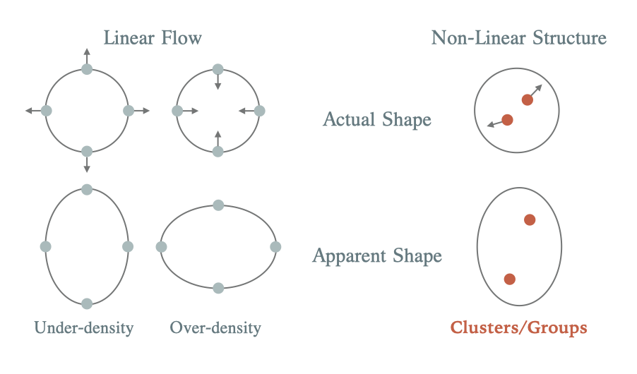
Figure 2: Illustration of redshift-space distortions: On the right, the figure illustrates the Kaiser effect, where on large scales, velocity flows into large overdensities compress the appearance of these structures along the line of sight. On the left, the figure illustrates the scenario on a smaller scale within galaxy groups and clusters. The random motions of galaxies within these compact environments result in an apparent elongation along the line of sight. This phenomenon is known as the "Fingers of God" effect.

To address the issue of redshift-space distortion in clustering galaxy groups, we propose modifying the Euclidean distance metric typically employed in OPTICS clustering algorithms. This modification aims to counteract the elongation effect along the line of sight arising from redshift distortion. The adjustment involves scaling the distance calculation’s line-of-sight(LOS) component.

The standard Euclidean distance between two points in a three-dimensional (3D) space is defined as:

$$D^{2}(u,v)=\sum_{i=1}^{n}(u_{i}-v_{i})^{2}\,,$$ (4)

where $u$ and $v$ represent the position vectors of the two points in space.

To address redshift-space distortion, we introduce a LOS scaling factor denoted as $s_{\mathrm{LOS}}$ for the line-of-sight component. Consequently, the modified distance metric, referred to as the Elongated Euclidean Distance, is computed as follows:

$$D_{\mathrm{Elongated}}^{2}(u,v,s_{\mathrm{LOS}})=d_{\mathrm{Transverse}}^{2}(u,v)+d_{\mathrm{LOS,\,scaled}}^{2}(u,v,s_{\mathrm{LOS}})\;.$$ (5)

The LOS component is calculated by projecting the difference vector:

$$d_{\mathrm{LOS}}(u,v)=\frac{\sum_{i=1}^{3}(u_{i}-v_{i})u_{i}}{\sqrt{\sum_{i=1}^{n}u_{i}^{2}}}\;.$$ (6)

Subsequently, this component is scaled by $s_{\mathrm{LOS}}$, representing the LOS scaling factor, to obtain the scaled LOS component:

$$d_{\mathrm{LOS,scaled}}(u,v,s_{\mathrm{LOS}})=s_{\mathrm{LOS}}\,d_{\mathrm{LOS}}(u,v)\;.$$ (7)

The final distance metric, the elongated Euclidean distance, incorporates this scaled LOS component, effectively compensating for the redshift-space distortion by "shortening" the distance along the line of sight.

Figure 3 illustrates the elongated Euclidean distance’s effect on the OPTICS clustering results. This adjustment transforms the sphere with an $\epsilon$-radius into an ellipse elongated along the LOS, enabling the inclusion of more distant galaxies along the LOS as possible neighbors. Consequently, this results in shorter core distances and deeper valleys in the reachability plot. Unlike direct modeling of redshift dispersion, this approach indirectly addresses and mitigates the underestimation issues associated with redshift-space distortions.

In practice, we have tested the effectiveness of this scaling adjustment. Figure 4 shows the clustering results of OPTICS in a subsample at redshift $z=0.10$, both with and without the scaling adjustment, and compares the predicted groups to the Y07 groups. The results demonstrate that redshift-space distortion significantly influences clustering outcomes, leading to a considerable underestimation along the LOS. By employing the elongated Euclidean distance, we have achieved a more precise prediction of galaxy groups, which improves both the detection of group shapes and the accuracy of membership. In the subsequent sections, we will refer to this OPTICS clustering method with the elongated Euclidean distance as scaled OPTICS (sOPTICS).

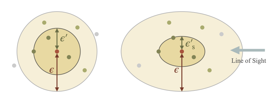
Figure 3: Illustration demonstrating the role of the LOS scaling factor $s_{\mathrm{LOS}}$ in our sOPTICS algorithm to mitigate redshift-space distortion.

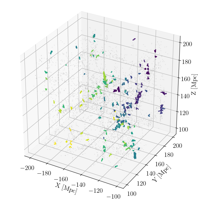
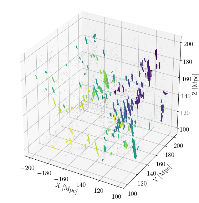
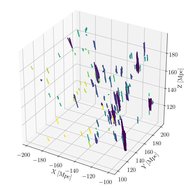
Figure 4: The left panel of the figure presents the result of the sOPTICS algorithm applied without any scaling adjustments. The middle panel presents the results of unscaled OPTICS, while the pairs of LOS distances have been scaled by a factor of $s_{\mathrm{LOS}}=0.2$. The right panel, in contrast, displays the actual galaxy groups as identified in the Y07 group catalog. In the left and middle panels of the figure, the gray points represent galaxies that the OPTICS and sOPTICS algorithm predicts as not belonging to any groups.

However, the effect of redshift-space distortion is not constant across different redshifts. A galaxy with a cosmological redshift $z_{\rm c}$ and a ’peculiar’ redshift $z_{\mathrm{p}}$ will appear to an observer to have an observed redshift $z$, as described by the equation:

$$(1+z)=(1+z_{\rm c})\left(1+z_{\mathrm{p}}\right)\;.$$ (8)

The approximation $z=z_{\rm c}+z_{\mathrm{p}}$ is only valid for small redshifts. Consequently, redshift-space distortion increasingly affects galaxy groups at higher redshifts. This stronger distortion necessitates more robust adjustments, specifically, smaller $s_{\mathrm{LOS}}$. Therefore, it is necessary to adjust the value of the LOS scaling factor $s_{\mathrm{LOS}}$ with redshift. To ascertain the proper values of $s_{\mathrm{LOS}}$ correcting for redshift-space distortions across varying redshift bins, in Section 4.3 we iteratively adjusted $z=z_{\rm c}+z_{\mathrm{p}}$ to optimize the concordance between our observations and the Y07 group catalog. Figure 5 illustrates how the optimal LOS scaling factor changes with redshift. It is clearly shown that the optimal LOS scaling factor decreases with higher redshifts, indicating that the Euclidean distance along the LOS is elongated more significantly. This trend is consistent with theoretical predictions.

In addition, the LOS scaling factor is also related to the values of $\epsilon$ itself. If the $\epsilon$ value is sufficiently large, all potential group members would be included, eliminating the need for elongation along the LOS. However, the redshift-space distortion predominantly impacts the distance measurements along the LOS. As Figure 1 demonstrates, employing larger $\epsilon$ values might reduce the identified groups’ purity. This reduction in purity occurs because a larger $\epsilon$ value causes the algorithm to excessively consider neighboring objects along the LOS and in the opposite direction, with little physical association. Considering the inherent noise and variability in the observed distribution of galaxies compared to their simulated counterparts, carefully adjusting the parameters $\epsilon$ and the corresponding $s_{\mathrm{LOS}}$ is essential. To address this, we have examined the relationship between the optimal sets of $s_{\mathrm{LOS}}$ and $\epsilon$. Our findings, detailed in Figure 10, reveal a well-defined optimal region for selecting these parameters. This optimal region ensures a balanced approach to grouping galaxies, optimizing both the purity of the groups and the inclusion of genuine group members, thus mitigating the effects of observational noise and distortion.

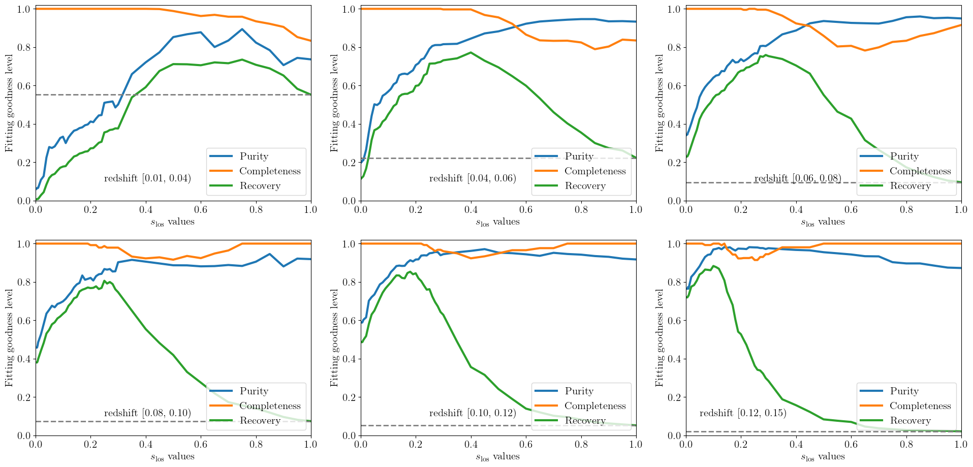
Figure 5: The dependence of purity, completeness, and recovery rate on the LOS scaling factor $s_{\mathrm{LOS}}$ across different redshifts for a specific sample defined by a right ascension range between 150 and 200 deg and a declination range between 10 and 60 deg. The grey dashed line highlights the baseline of recovery rate achieved by the original OPTICS method when $s_{\mathrm{LOS}}=1$.

4.3 Choices of Hyperparameter Values

To determine the optimal hyperparameter values for FoF and sOPTICS, similar to our approach for refining $s_{\mathrm{LOS}}$, we initiate the optimization process by aligning them with the Y07 group catalog, which serves as our reference model. Incorporating the LOS scaling factor $s_{\mathrm{LOS}}$ into sOPTICS, the algorithm now boasts five hyperparameters requiring optimization, whereas FoF requires only two: linking length $l$ and $M_{\rm min}$. It is important to note that the evaluation criteria diverge from the tests conducted on simulated galaxy catalogs as described in Section 3. This divergence stems from astrophysical studies on galaxy groups and clusters typically prioritize those with substantial membership. Given that merely 1.78% of groups consist of at least five galaxy members (totaling 8,427 out of 472,416 groups in Y07 catalog), we suggest a refined adjustment to the definition of the recovery rate, strategically assigning heightened weight to groups exhibiting a greater abundance of members:

$$F_{\mathrm{R}}=\sum^{\mathcal{N}}_{i=0}\delta_{i}\times\frac{\text{Number of galaxies in group $i$}}{\text{Total number of non-isolated galaxies}}\,,$$ (9)

where $\mathcal{N}$ is the total number of true groups in Y07, and:

$$\delta_{i}=\begin{cases}1,&\text{if group $i$ is simultaneously pure and complete,}\\ 0,&\text{otherwise.}\end{cases}$$ (10)

Leveraging the abundance-weighted recovery rate as a criterion for optimization allows us to prioritize identifying giant clusters in our analyses. When comparing different sets of parameters, preference is given to those configurations that enhance the recovery of a larger number of giant clusters, as cataloged in Y07.

To fine-tune the hyperparameters, we select ten subsamples from low redshift galaxies ($z<0.05$), each with a cubic side length of 100 Mpc. Then, we first identify the optimal values of hyperparameters of FoF, as well as sOPTICS with a constant $s_{\mathrm{LOS}}$, which maximizes the abundance-weighted recovery rate, as detailed in Table 2. Using these hyperparameters, we achieved a maximum recovery rate of $F_{\mathrm{R}}=0.8$ for FoF and 0.76 for sOPTICS. It is important to note that for sOPTICS, although the recovery rate of 0.76 wasn’t the peak for every individual test subsample—with the highest rate reaching 0.89 in certain scenarios—these hyperparameters yield the most consistent and accurate predictions of BCGs across the board, as elaborated in Section 5.1. Thus, we adopted this set of hyperparameters for sOPTICS as the most suitable choice, balancing overall performance across various testing conditions.

Maintaining the optimal hyperparameters identified earlier, we proceeded to select subsamples of 100 Mpc within each redshift bin to fit the optimal value for $s_{\mathrm{LOS}}$ that effectively mitigates redshift space distortion, as detailed in Table 3. Here we note that, after extensive testing, we meticulously determined the delineation of redshift bins with prior knowledge from the Y07 group catalog to prevent the segmentation of giant clusters across two bins, ensuring a more coherent and accurate analysis.

FoF		sOPTICS
$l$	$M_{\mathrm{min}}$	$\epsilon$	$N_{\mathrm{min}}$	$M_{\mathrm{min}}$	$\xi$
1.6	2	1.2	5	5	0.9

Table 2: The hyperparameters for the FoF and sOPTICS algorithm, as applied to the entire galaxy sample described in Section 4.1. It is important to note that, due to the magnitude limit constraints of the SDSS survey and local incompleteness factors, the values of $N_{\mathrm{min}}$ were adjusted based on the redshifts of the galaxies. For galaxies with redshifts $z<0.10$, we utilized the hyperparameters as listed, and for galaxies at higher redshifts, we modified the $N_{\mathrm{min}}$ to 4.

Redshift bins	0.01 - 0.04	0.04 - 0.06	0.06 - 0.08	0.08 - 0.10
$s_{\mathrm{LOS}}$	0.5	0.4	0.35	0.3
Redshift bins	0.10 - 0.12	0.12 - 0.15	0.15 - 0.20
$s_{\mathrm{LOS}}$	0.19	0.08	0.01

Table 3: The best-fitted values of the LOS scaling factor, $s_{\mathrm{LOS}}$, across various redshifts. The analysis is constrained by other parameters as listed in Table 2. It is important to note that the bin settings provided here represent approximate values. In our practice, slight adjustments are made to the settings of redshift bins to prevent significant groups from being split across two bins.

4.4 Basic Results

With the optimal values for hyperparameters and the LOS scaling factor listed in Table 2 and 3, the overall abundance-weighted recovery rate for galaxy groups using the sOPTICS algorithm is 74.9%, with the abundance-weighted purity of 86.6% and completeness of 96.9%. The total number of identified groups is 12,196. Meanwhile, the soft recovery rate stands at 69.0%, indicating that we can precisely identify 5,811 galaxy groups, with two-thirds of their member galaxies matching those of the true groups identified in Y07 and covering more than half of the actual members, out of a total of 8,427 true groups. In contrast, the FoF algorithm achieved a soft recovery rate of 64.7%, while with a purity of 46.3% and completeness of 78.9%. The total number of identified groups using FoF is 95,732, which is much larger than the number identified by sOPTICS, indicating a very low efficiency identification and non-negligible contamination in the detected group. Therefore, by incorporating the LOS scaling factor, we significantly enhanced the precision of the sOPTICS algorithm’s predictions. Consequently, in identifying galaxy groups and clusters, sOPTICS performs comparably to, and in some cases slightly better than, FoF when parameters are tuned based on sub-samples.

We also visually inspect the large galaxy groups and clusters with the aid of the color-magnitude relation of the groups and clusters, $r$-magnitude versus $(g-r)$ Color diagrams were made for field galaxies and cluster + field galaxies in each SDSS square. The stacked field galaxy maps were subtracted from the stacked cluster galaxy maps, taking into account the relative areas (within 10 Mpc). In the color-magnitude diagram, the presence of a clear red sequence indicates a real galaxy group, as opposed to just a chance alignment of field galaxies. Figure 6 shows the color–magnitude diagrams for the largest galaxy group in Y07 and the corresponding group predicted by sOPTICS, which is also the largest one in prediction. The maps reveal a distinct trend in color-magnitude space, resembling a cluster red sequence. Remarkably, over two-thirds of the member galaxies, including the BCG, are accurately predicted.

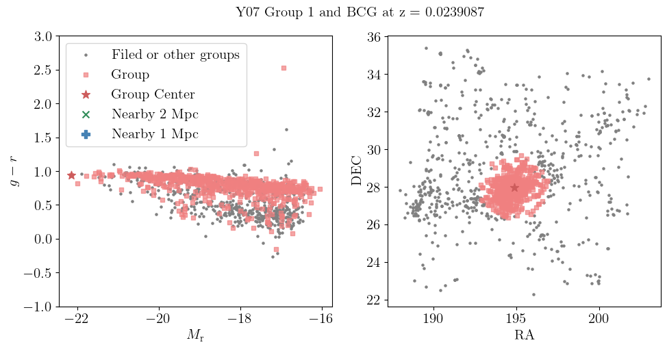
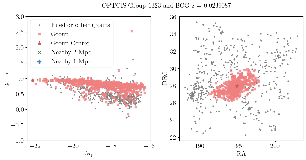
Figure 6: Color–magnitude diagrams (left panels) and projected distributions (right panels) of SDSS galaxies. The upper panels present galaxies in the largest group from the Y07 catalog (group ID 1) and field galaxies surrounding the group center within a 10 Mpc radius. The bottom panels present the corresponding group predicted by sOPTICS and its surrounding field galaxies. These color-magnitude diagrams reveal a tight correlation in the color-magnitude space, closely resembling a cluster red sequence. Meanwhile, the original group from the Y07 catalog is effectively predicted by sOPTICS, exhibiting high completeness, and the BCG of this group is precisely identified.

5 Capability of Clustering Algorithms

With the aid of the LOS scaling factor, we have successfully recovered nearly 70 % of galaxy groups from the Y07 group catalog. This is a significant improvement considering the complexity and time-intensive nature of the Y07 catalog identification process.

In Yang et al. 2007, initially, the FoF algorithm with very short linking lengths in redshift space was used to identify preliminary groups that likely represent the central regions of these clusters. The geometrically determined, luminosity-weighted centers of all FoF-identified groups with at least two members were designated potential group centers. Galaxies not associated with these FoF groups were also treated as potential centers. Each group’s characteristic luminosity, $L_{19.5}$, was then calculated to facilitate a meaningful group comparison. This luminosity was used to assign a halo mass to each group, which allowed for the estimation of the group’s halo radius and velocity dispersion. Subsequent updates to group memberships were guided by a probability density function calculated in redshift space around each group’s center, considering halo properties. This iterative process – consisting of updating group memberships, recalculating centers, and refining the $M_{h}/L_{19.5}$ to $L_{19.5}$ relationship – continued until the group dynamics stabilized, usually after a few iterations. Their comprehensive method thus enhanced the understanding of galaxy group dynamics and composition, overcoming limitations posed by redshift space distortions.

In comparison, our method scaled OPTICS, takes only about one hour on average and involves a straightforward process, yet it achieves high recovery rates of the Y07 catalog. Therefore, the primary strength of sOPTICS lies in its efficiency in identifying galaxy groups from large surveys with very low computational costs. Moreover, it is particularly sensitive to detecting large clusters, achieving high accuracy in identifying their members. This combination of speed, simplicity, and precision makes sOPTICS an advantageous tool for astrophysical studies requiring the analysis of extensive data sets.

5.1 Performance of finding BCGs

As demonstrated, sOPTICS can effectively detect large clusters with precise member identification, including the BCGs. To evaluate the performance of our sOPTICS method in identifying BCGs from a galaxy survey, we conducted a comparative test against a recent BCGs sample from Hsu et al. (2022, hereafter Hsu22). Their parent BCG sample of 4,033 galaxy clusters is also extracted from the group catalog of Y07 with applying a cut in the cluster mass $M_{180m}\geqslant 10^{14}h^{-1}M_{\odot}$. By cross-matching BCG candidates with the 8,113 galaxies released in the ninth Product Launch (MPL-9) of the Mapping Nearby Galaxies at Apache Point Observatory (MaNGA Bundy et al., 2014), they identified 128 BCGs situated within a redshift range of $z=0.02-0.15$. These clusters are all detected in the X-rays by Wang et al. (2014), which provides a cluster catalog with X-ray luminosity from ROSAT All Sky Survey. However, Y07 primarily select BCGs based on luminosity, occasionally resulting in the selection of spiral galaxies as BCG candidates. Therefore, Hsu22 implemented an additional visual selection process: if the BCG candidates show a spiral morphology or do not represent the most luminous galaxy on the red sequence, alternative candidates would considered. The cluster would be excluded if no superior candidate exists or MaNGA has not observed the more suitable candidate. As a result, 121 BCGs have been visually confirmed, of which 118 were originally part of the Y07 catalog.

While traditionally thought to be close to the center, recent studies have shown that the BCG may not always be at the cluster’s center, with a fraction of BCGs being non-central depending on the halo mass (Chu et al., 2021). This deviation from being at the center is due to different definitions of BCGs based on their luminosity or mass, regardless of their position within the cluster. Therefore, in this work, we identify BCGs based solely on their $r$ band magnitude, irrespective of their spatial position in the cluster.

Using the best-fitted parameters and the LOS scaling factor listed in Table 2 and 3, we successfully identified 115 BCGs consistent with the 118 BCGs identified in Hsu22. The spatial distribution of the galaxy clusters corresponding to these BCGs in redshift and right ascension (RA) space is illustrated in Figure 7. Only three relatively small clusters failed to be predicted by sOPTICS. Figure 8 shows a segment of the reachability plot for scaled OPTICS, where the galaxy clusters appear as distinct, deep valleys. The gray areas represent isolated field galaxies that are significantly distanced from others. The bottom panel shows a specific example cluster’s reachability distances and neighbors, including a BCG recovered from the Hsu22 sample. It is shown that these density-based clustering methods, such as OPTICS and sOPTICS, have given us a clear and straightforward picture of the position of BCGs in clusters. In this particular case, the BCG is located precisely at the densest part of the region, indicating a perfect alignment with the cluster’s center of gravity. However, it is also evident from other commonly detected cases (highlighted as yellow spots in the plot) that the BCGs are not always situated at the densest part of the cluster. This variation highlights the diversity in the spatial distributions of BCGs and explains why our sOPTICS method did not successfully predict three BCGs.

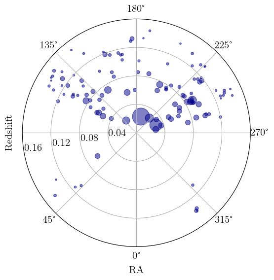
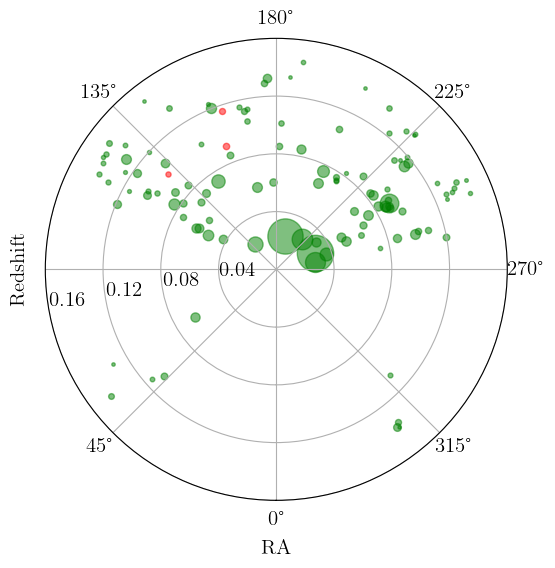
Figure 7: Distribution of both recovered and unrecovered BCGs from Hsu22 within their respective galaxy groups visualized in the RA-redshift space. The left panel shows the distribution of galaxy groups in Y07 catalog. In the right panel, green dots represent the galaxy groups successfully identified by sOPTICS. And red dots represent the groups that remained undetected by sOPTICS. The size of these dots is scaled to correspond to the member density of each group.

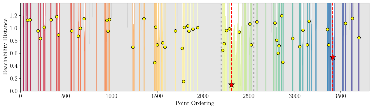
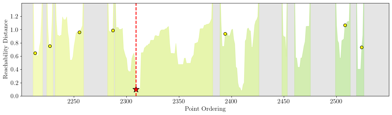
Figure 8: The reachability plot for galaxy groups from a sample covering a $30^{2}\,\deg^{2}$ sky area within the redshift range $0.7<z<0.8$. The colors highlight different clusters as determined by the clustering process described in Section 4.2. The top panel displays the complete reachability plot of this sample, while the bottom panel focuses on a specific section marked by grey dashed lines in the top panel. Light grey regions in each panel indicate isolated galaxies. Yellow points represent the brightest galaxies identified in each group. The red line and red star marker denote the reachability distance of the BCGs identified in Hsu22 and those successfully recovered in our analysis, respectively.

5.2 sOPTICS: a robust group and BCG finder

In employing the scaled OPTICS clustering algorithm to identify galaxy clusters, the hyperparameters $\epsilon$ (the maximum radius for neighborhood density estimation), $N_{\mathrm{min}}$ (the minimum number of points required to form a cluster), and the LOS scaling factor crucially influence the results, as detailed in Section 3. These parameters are pivotal in determining reachability distances and adjusting the algorithm to mitigate the effects of redshift-space distortion.

Although one might expect the clustering outcome to be highly sensitive to parameter variations, sOPTICS shows resilience by exhibiting an optimal range for their values. This finding is illustrated in Figures 9 and 10, where the interdependence of $\epsilon$ and $N_{\mathrm{min}}$, as well as $\epsilon$ and $s_{\mathrm{LOS}}$, is presented. Notably, a clear correlation emerges between $\epsilon$ and $N_{\mathrm{min}}$; as $\epsilon$ increases, $N_{\mathrm{min}}$ also needs to be adjusted upward to maintain effective clustering. Essentially, to preserve the purity of the clusters identified by the sOPTICS algorithm, the criteria must shift toward identifying denser and larger clusters as the $\epsilon$ threshold is raised. The positive correlation suggests that $\epsilon^{3}\propto N_{\mathrm{min}}$ aligns with theoretical expectations. Theoretically, this adjustment ensures that the increase in the neighborhood radius does not lead to the inclusion of outlier points or less dense areas. Thus $N_{\mathrm{min}}$ should correlate with the volume of space encompassed within $\epsilon$, which implies a cubic relationship ($\epsilon^{3}$).

Adjustments in the LOS scaling factor, $s_{\mathrm{LOS}}$, which modifies how the LOS distance is shortened, exhibit a nearly linear relationship with $\epsilon$, such that $\epsilon\propto s_{\mathrm{LOS}}$. This relationship implies that increasing $\epsilon$ expands the effective search radius in the clustering algorithm, thereby capturing more of the spatial distribution of galaxies affected by redshift space distortion. Consequently, it reduces the necessity to stretch the LOS distance to mitigate these distortions.

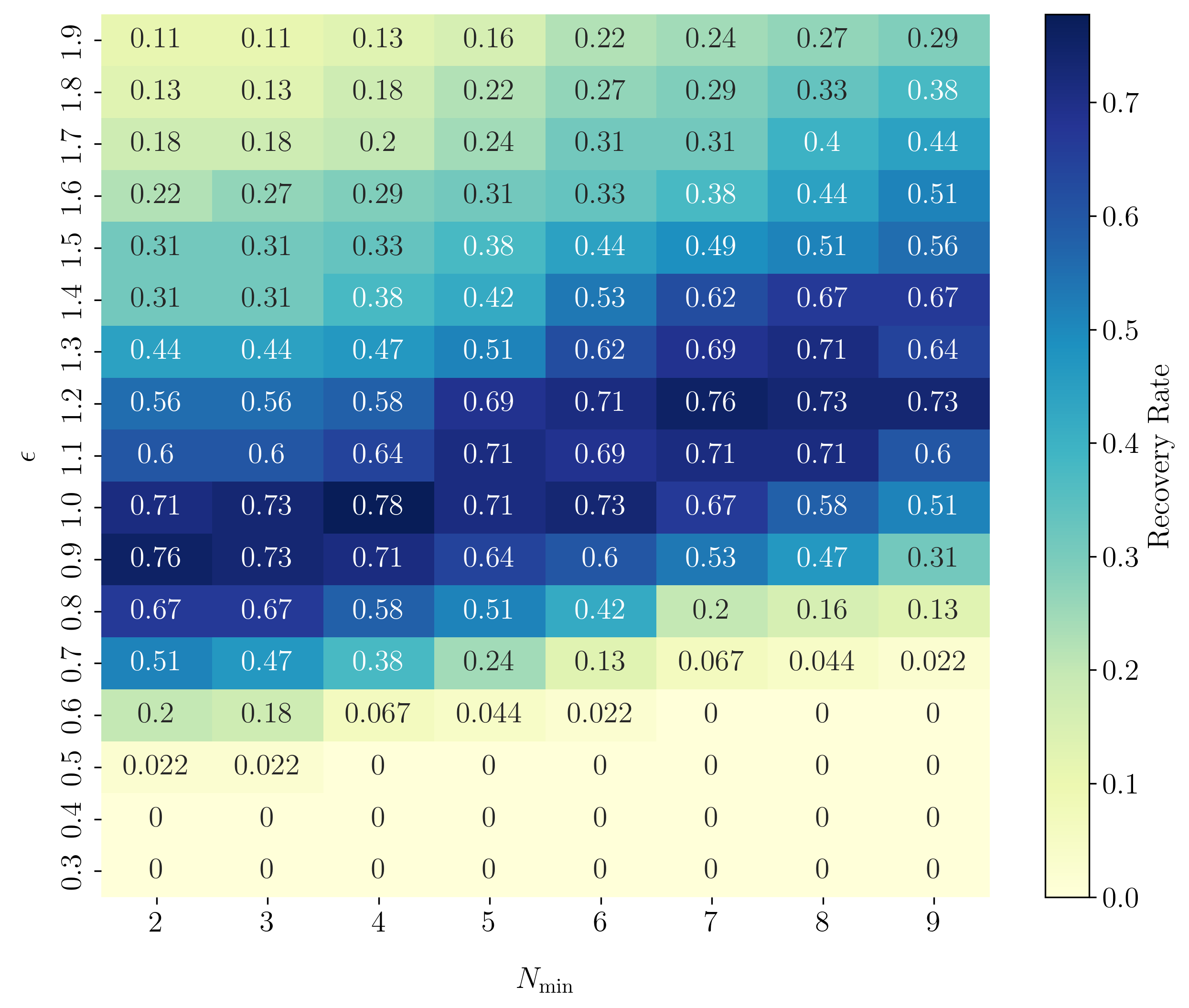
Figure 9: The results of clustering for various pairs of values of $\epsilon$ and $N_{\mathrm{min}}$. The color bar represents the weighted recovery rate of the predicted groups relative to a subsample from the Y07 groups catalog, covering a $30^{2}\,\deg^{2}$ sky area within the redshift range $0.7<z<0.8$.

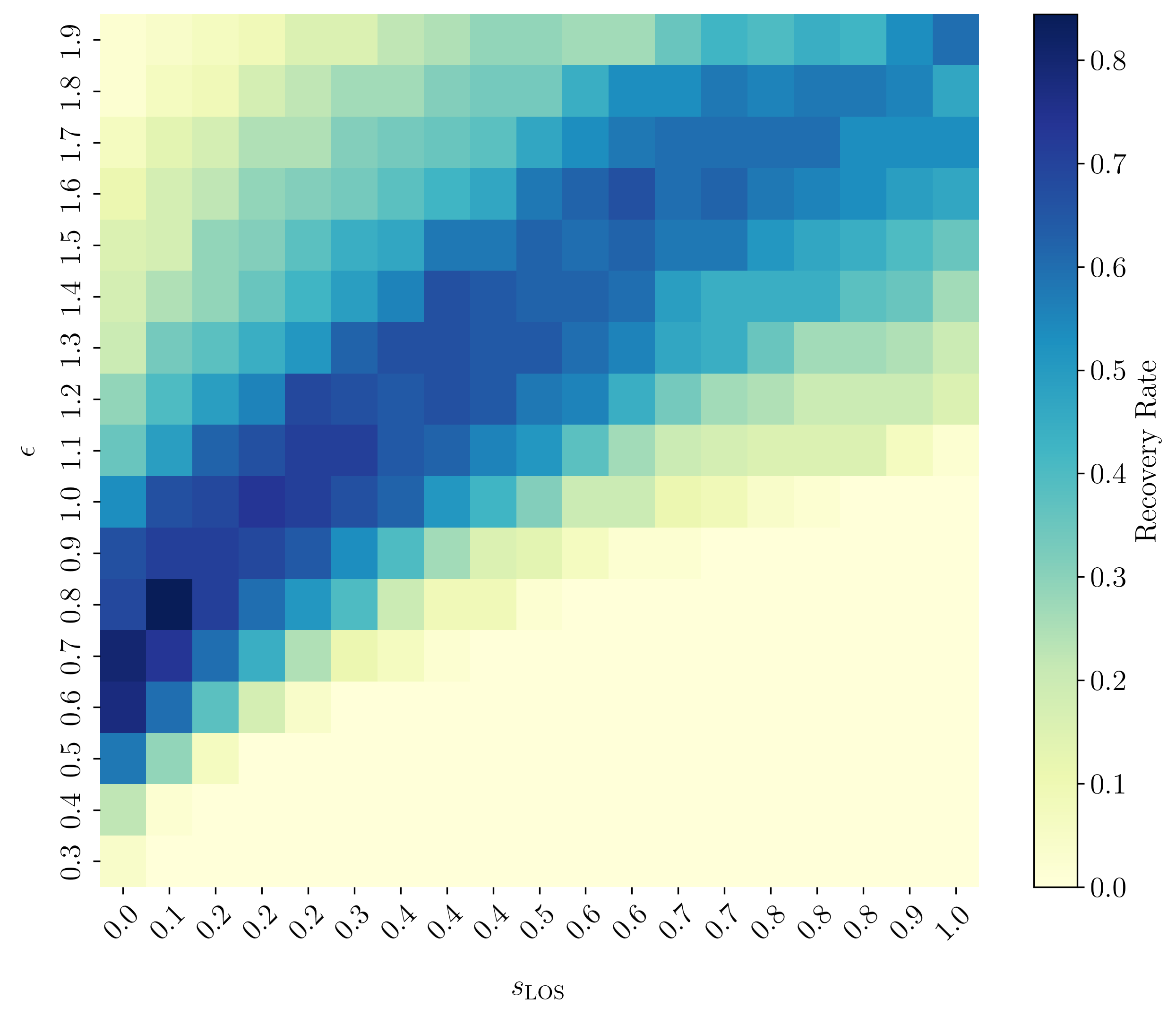
Figure 10: As Fig. 9, but showing the results of clustering for various pairs of values of $s_{\mathrm{LOS}}$ and $\epsilon$.

These relationships underscore the interconnected nature of these parameters and their collective impact on optimizing cluster detection and recovery rates. They are fundamental in understanding how changes in one parameter necessitate adjustments in the other to maintain the purity and completeness of clustering outcomes. Specifically, within a certain redshift range, selecting values for these three parameters from this optimal range can yield galaxy groups with a high recovery rate comparable to those obtained from reliable group catalogs that require complex and computationally intensive processes. The optimal ranges depicted in Figures 9 and 10 also identify a potential characteristic number density for categorizing galaxies in a survey as a group. Given the similar local completeness of the survey, this characteristic number density of galaxy groups can be applied to other observations. This consideration is pivotal when choosing hyperparameter values.

However, given the current redshift range of the observed data, the relationships observed between $\epsilon$, $N_{\mathrm{min}}$, and $s_{\mathrm{LOS}}$ are preliminary and roughly empirical. To more precisely define these relationships and understand the characteristic number density, a comprehensive analysis using both real-world data and mock catalogs is crucial. This approach would help determine whether the observed linear trend between $\epsilon$ and $s_{\mathrm{LOS}}$ is an artifact of the specific dataset used in this study or if it reflects a more general characteristic applicable across different galaxy cluster distributions. Furthermore, a theoretical exploration into the dynamics of galaxy clusters and their spatial density distributions, similar to the approach taken by Y07, should be considered. Such studies would provide deeper insights into the viability of sOPTICS methods and enrich our understanding of the underlying physical properties that govern the formation and evolution of galaxy clusters.

In addition, given that BCGs are typically located near the densest part of a cluster, sOPTICS, which specifically focuses on dense patterns within a survey, naturally excels as a tool for locating BCGs. It indeed has shown promising results in tests against the Hsu22 sample (see Section 5.1. Therefore, for researchers primarily interested in identifying BCGs, sOPTICS can be effectively employed with a specific set of parameters tailored for very dense groups: small values of $\epsilon$, large $N_{\mathrm{min}}$, and reasonable values of $s_{\mathrm{LOS}}$. This setup allows for rapidly identifying potential BCG candidates from large and complex surveys. In contrast, the FoF can not efficiently identify purely large clusters without contaminating smaller ones due to small values for the linking length. Still, It is important to note that while BCGs are the most luminous galaxies within their clusters, they may not always coincide with the cluster’s geometric center, which is influenced by both the geometry and the luminosity of member galaxies (Skibba et al., 2011). Accurate identification of BCGs requires a meticulous selection process that considers factors such as brightness, proximity to the cluster center, distinctive features, and corroborative data from various observational sources. Subsequent verification using additional observations, such as X-ray and optical surveys, should be done on the candidates to confirm the true BCGs.

6 Summary and Conclusion

This study evaluated the effectiveness of eight popular clustering algorithms in data science for identifying galaxy groups and clusters through tests involving comparisons with both simulations and existing reliable group catalogs. Our findings indicate that the FoF and sOPTICS algorithms are robust galaxy group finders. Remarkably, our sOPTICS method exhibits considerable stability and flexibility in the choice of hyperparameter values and, enhanced by the line-of-sight scaling factor to mitigate redshift-space distortion, outperforms FoF in both efficiency and accuracy in identifying the most geometrically dense parts of galaxy groups and in pinpointing BCGs from large surveys.

We conclude that scaled OPTICS and FoF are comparably effective, with sOPTICS demonstrating high purity and recovery rates. While FoF can be faster and more computationally efficient, especially for large datasets – an advantage in astronomical computations – its performance heavily depends on the choice of linking length. Despite this dependency, FoF, as a popular and classical clustering method in astrophysics, remains particularly effective for low redshift surveys where redshift space distortion is less significant.

sOPTICS is particularly noteworthy for three reasons: i) It demonstrates robustness to a wide range of hyperparameter values. Most importantly, there are two empirical relationships involving its hyperparameters $\epsilon$, $N_{\mathrm{min}}$, and $s_{\mathrm{LOS}}$ enabling us to estimate a reasonable range of values to achieve reliable clustering results. ii) Unlike many clustering algorithms, sOPTICS does not segment data into clusters during its initial run. Instead, it generates a reachability plot illustrating distances to the nearest neighbor within the $\epsilon$-neighborhood. Clusters are subsequently identified based on the valleys within this plot. This approach allows sOPTICS to be less sensitive to hyperparameter settings as long as they are sufficient to capture significant structures in the data. iii) sOPTICS primarily focuses on the densest parts of a dataset, where the BCGs are often located. This focus makes it naturally efficient in identifying BCGs. By setting even extreme hyperparameter values, researchers can easily identify reliable BCG candidates for further analysis, simplifying the process compared to more complex galaxy group-finding methods.

Looking ahead, we anticipate leveraging richer and more precise galaxy data from sources such as the Dark Energy Spectroscopic Instrument (DESI, Dey et al., 2019) and other ongoing large-scale spectroscopic surveys. This will enable more realistic treatments in hyperparameter modeling, especially for galaxy groups and clusters at higher redshifts. Furthermore, we aim to refine the relationships and potential characteristic numbers suggested by the hyperparameters $\epsilon$, $N_{\mathrm{min}}$, and $s_{\mathrm{LOS}}$ in sOPTICS.

Data Availability

The data underlying this paper is publicly available at http://sdss.physics.nyu.edu/vagc/ and https://gax.sjtu.edu.cn/data/Group.html. The derived data generated in this research will be shared on a reasonable request to the first author.

References

- Abazajian et al. (2009) Abazajian K. N., et al., 2009, ApJS, 182, 543
- Ankerst et al. (1999) Ankerst M., Breunig M. M., Kriegel H.-P., Sander J., 1999, in Proceedings of the 1999 ACM SIGMOD International Conference on Management of Data. SIGMOD ’99. Association for Computing Machinery, New York, NY, USA, pp 49–60, doi:10.1145/304182.304187
- Blanton et al. (2005) Blanton M. R., et al., 2005, AJ, 129, 2562
- Bottou & Bengio (1994) Bottou L., Bengio Y., 1994, in Advances in Neural Information Processing Systems. MIT Press
- Bouchet et al. (1995) Bouchet F. R., Colombi S., Hivon E., Juszkiewicz R., 1995, A&A, 296, 575
- Brauer et al. (2022) Brauer K., Andales H. D., Ji A. P., Frebel A., Mardini M. K., Gómez F. A., O’Shea B. W., 2022, ApJ, 937, 14
- Buchert (1992) Buchert T., 1992, MNRAS, 254, 729
- Bundy et al. (2014) Bundy K., et al., 2014, ApJ, 798, 7
- Campello et al. (2013) Campello R. J. G. B., Moulavi D., Sander J., 2013, in Pei J., Tseng V. S., Cao L., Motoda H., Xu G., eds, Advances in Knowledge Discovery and Data Mining. Springer, Berlin, Heidelberg, pp 160–172, doi:10.1007/978-3-642-37456-2_14
- Campello et al. (2015) Campello R. J. G. B., Moulavi D., Zimek A., Sander J., 2015, ACM Trans. Knowl. Discov. Data, 10, 1
- Castro-Ginard et al. (2018) Castro-Ginard A., Jordi C., Luri X., Julbe F., Morvan M., Balaguer-Núñez L., Cantat-Gaudin T., 2018, A&A, 618, A59
- Castro-Ginard et al. (2020) Castro-Ginard A., et al., 2020, A&A, 635, A45
- Chi et al. (2023) Chi H., Wang F., Wang W., Deng H., Li Z., 2023, ApJS, 266, 36
- Chu et al. (2021) Chu A., Durret F., Márquez I., 2021, A&A, 649, A42
- Croton et al. (2006) Croton D. J., et al., 2006, MNRAS, 365, 11
- De Lucia & Blaizot (2007) De Lucia G., Blaizot J., 2007, MNRAS, 375, 2
- Dehghan & Johnston-Hollitt (2014) Dehghan S., Johnston-Hollitt M., 2014, AJ, 147, 52
- Dempster et al. (1977) Dempster A. P., Laird N. M., Rubin D. B., 1977, Journal of the Royal Statistical Society: Series B (Methodological), 39, 1
- Dey et al. (2019) Dey A., et al., 2019, AJ, 157, 168
- Duann et al. (2023) Duann Y., Tian Y., Ko C.-M., 2023, RAS Techniques and Instruments, 2, 649
- Ester et al. (1996) Ester M., Kriegel H.-P., Sander J., Xu X., 1996, in Proceedings of the Second International Conference on Knowledge Discovery and Data Mining. KDD’96. AAAI Press, Portland, Oregon, pp 226–231
- Foulds (1991) Foulds L. R., 1991, Graph theory applications. Uniersitext, Springer-Verlag,, New York:
- Fuentes et al. (2017) Fuentes S. A. S., Ridder J. D., Debosscher J., 2017, A&A, 599, A143
- Hsu et al. (2022) Hsu Y.-H., et al., 2022, ApJ, 933, 61
- Huchra & Geller (1982) Huchra J. P., Geller M. J., 1982, ApJ, 257, 423
- Kaiser (1987) Kaiser N., 1987, MNRAS, 227, 1
- Kauffmann & Haehnelt (2000) Kauffmann G., Haehnelt M., 2000, MNRAS, 311, 576
- Kluge et al. (2020) Kluge M., et al., 2020, ApJS, 247, 43
- Lauer (1988) Lauer T. R., 1988, ApJ, 325, 49
- MacQueen (1967) MacQueen J., 1967, Proceedings of the Fifth Berkeley Symposium on Mathematical Statistics and Probability, Volume 1: Statistics, 5.1, 281
- Marulli et al. (2017) Marulli F., Veropalumbo A., Moscardini L., Cimatti A., Dolag K., 2017, A&A, 599, A106
- McConnachie et al. (2005) McConnachie A. W., Irwin M. J., Ferguson A. M. N., Ibata R. A., Lewis G. F., Tanvir N., 2005, MNRAS, 356, 979
- McInnes et al. (2017) McInnes L., Healy J., Astels S., 2017, Journal of Open Source Software, 2, 205
- Moore et al. (1998) Moore B., Governato F., Quinn T., Stadel J., Lake G., 1998, ApJ, 499, L5
- Ng et al. (2001) Ng A., Jordan M., Weiss Y., 2001, in Advances in Neural Information Processing Systems. MIT Press
- Olave-Rojas et al. (2023) Olave-Rojas D. E., Cerulo P., Araya-Araya P., Olave-Rojas D. A., 2023, MNRAS, 519, 4171
- Oliver et al. (2021) Oliver W. H., Elahi P. J., Lewis G. F., Power C., 2021, MNRAS, 501, 4420
- Onions et al. (2012) Onions J., et al., 2012, MNRAS, 423, 1200
- Press & Davis (1982) Press W. H., Davis M., 1982, ApJ, 259, 449
- Quintana & Lawrie (1982) Quintana H., Lawrie D. G., 1982, AJ, 87, 1
- Reid & White (2011) Reid B. A., White M., 2011, MNRAS, 417, 1913
- Reid et al. (2012) Reid B. A., et al., 2012, MNRAS, 426, 2719
- Sander et al. (1998) Sander J., Ester M., Kriegel H.-P., Xu X., 1998, Data Mining and Knowledge Discovery, 2, 169
- Sankhyayan et al. (2023) Sankhyayan S., et al., 2023, ApJ, 958, 62
- Shin et al. (2022) Shin J., Lee J. C., Hwang H. S., Song H., Ko J., Smith R., Kim J.-W., Yoo J., 2022, ApJ, 934, 43
- Skibba et al. (2011) Skibba R. A., van den Bosch F. C., Yang X., More S., Mo H., Fontanot F., 2011, MNRAS, 410, 417
- Sohn et al. (2021) Sohn J., Geller M. J., Hwang H. S., Diaferio A., Rines K. J., Utsumi Y., 2021, ApJ, 923, 143
- Springel (2005) Springel V., 2005, MNRAS, 364, 1105
- Springel et al. (2001) Springel V., White S. D. M., Tormen G., Kauffmann G., 2001, MNRAS, 328, 726
- Springel et al. (2005) Springel V., et al., 2005, Nature, 435, 629
- Tago et al. (2008) Tago E., Einasto J., Saar E., Tempel E., Einasto M., Vennik J., Müller V., 2008, A&A, 479, 927
- Thanjavur et al. (2010) Thanjavur K., Crampton D., Willis J., 2010, ApJ, 714, 1355
- Tian et al. (2021) Tian Y., Cheng H., McGaugh S. S., Ko C.-M., Hsu Y.-H., 2021, ApJ, 917, L24
- Tian et al. (2024) Tian Y., Ko C.-M., Li P., McGaugh S., Poblete S. L., 2024, A&A, 684, A180
- Turner & Gott (1976) Turner E. L., Gott III J. R., 1976, ApJS, 32, 409
- Wang et al. (2014) Wang L., et al., 2014, MNRAS, 439, 611
- Ward (1963) Ward J. H., 1963, Journal of the American Statistical Association, 58, 236
- White & Rees (1978) White S. D. M., Rees M. J., 1978, MNRAS, 183, 341
- White et al. (2015) White M., Reid B., Chuang C.-H., Tinker J. L., McBride C. K., Prada F., Samushia L., 2015, MNRAS, 447, 234
- Yang et al. (2005) Yang X., Mo H. J., Jing Y. P., van den Bosch F. C., 2005, MNRAS, 358, 217
- Yang et al. (2007) Yang X., Mo H. J., van den Bosch F. C., Pasquali A., Li C., Barden M., 2007, ApJ, 671, 153
- von Luxburg (2007) von Luxburg U., 2007, Stat Comput, 17, 395